Fast Hyperparameter Calibration of Sparsity Enforcing Penalties in Total Generalised Variation Penalised Reconstruction Methods for XCT Using a Planted Virtual Reference Image

Abstract

The reconstruction problem in X-ray computed tomography (XCT) is notoriously difficult in the case where only a small number of measurements are made. Based on the recently discovered Compressed Sensing paradigm, many methods have been proposed in order to address the reconstruction problem by leveraging inherent sparsity of the object’s decompositions in various appropriate bases or dictionaries. In practice, reconstruction is usually achieved by incorporating weighted sparsity enforcing penalisation functionals into the least-squares objective of the associated optimisation problem. One such penalisation functional is the Total Variation (TV) norm, which has been successfully employed since the early days of Compressed Sensing. Total Generalised Variation (TGV) is a recent improvement of this approach. One of the main advantages of such penalisation based approaches is that the resulting optimisation problem is convex and as such, cannot be affected by the possible existence of spurious solutions. Using the TGV penalisation nevertheless comes with the drawback of having to tune the two hyperparameters governing the TGV semi-norms. In this short note, we provide a simple and efficient recipe for fast hyperparameters tuning, based on the simple idea of virtually planting a mock image into the model. The proposed trick potentially applies to all linear inverse problems under the assumption that relevant prior information is available about the sought for solution, whilst being very different from the Bayesian method.

1. Introduction

1.1. Motivations

X-ray computed tomography (XCT) is increasingly used as a non-destructive evaluation tool to inspect industrial and medical components [1]. Conventional XCT using analytical reconstruction algorithms require scans with thousands of projection images, which is a time-consuming process. After the discretisation stage, the mathematical model is as follows: a number of measurements is collected in a vector y, and the operator which sends the original image $x^0$ to the vector of measurements, denoted by $\mathcal{A}$, enters the model as described in the following equation

$$\begin{array}{cc}\hfill y& =\mathcal{A}\left(x^0\right)+\zeta ,\hfill \end{array}$$

(1)

where $\zeta$ is the observation noise vector, usually assumed i.i.d. Gaussian $\mathcal{N}(0,{\sigma }^2)$, with variance ${\sigma }^2$. The recent breakthroughs of sparse reconstruction theory, better known as Compressed Sensing [2,3,4,5,6], enriched by algorithmic improvements such as in [7], or [8,9] where the problem of not knowing the noise variance is addressed, have provided a better understanding of how sparsity promoting penalisations could be devised in order to achieve accurate reconstruction using a very small number of projections.

Let us denote by $\mathsf{\Phi }$ the matrix whose columns represent the discretised Fourier, wavelet or shearlet basis elements, into which the original image’s decomposition is known to be sparse, or almost sparse (which in the approximation theoretic terminology is described as having a small best K-term approximation error decay as a function of K in these bases). The optimisation problem resulting from this modelling is often set up as a penalised least-squares problem of the form

$$\begin{array}{cc}\hfill \widehat{x}& ={\mathrm{argmin}}_{x\in {\mathbb{R}}^p}\frac{1}{2}{\parallel y-\mathcal{A}\left(x\right)\parallel }_2^2+\lambda p\left(\mathsf{\Phi }x\right)\hfill \end{array}$$

(2)

where $p\left(c\right)$ is a penalisation function which promotes sparsity of the vector c to which it is applied. Although the most natural penalisation is obtained by taking p to be the sparsity, i.e., the number of non-zero components, this choice is rarely adopted because of its non-convexity and the fact that the resulting optimisation problem (2) becomes computationally intractable [10]. Compressed Sensing theory developed tools which permitted the understanding of when sparsity could be profitably replaced with the ${\ell }_1$-norm, i.e., $p\left(c\right)={\parallel c\parallel }_1$, or $p\left(c\right)={\parallel c\parallel }_{TV}$, where $TV$ stands for Total Variation, which is a semi-norm (due to the fact ${\parallel c\parallel }_{TV}=0$ does not imply that $c=0$) defined as the ${\ell }_1$ norm of the vector of local differences of the components of c, i.e., $p\left(c\right)={\parallel \nabla c\parallel }_1$, where ∇ denotes the gradient, which readily extends to 2D or 3D objects. The main reason for these choices is that the resulting penalisation functional is convex and many efficient algorithms have been devised for such problems [11,12,13]. Oftentimes, different penalties are combined for promoting various properties of the reconstructed object and the resulting problem becomes

$$\begin{array}{cc}\hfill \widehat{x}& ={\mathrm{argmin}}_{x\in {\mathbb{R}}^p}\frac{1}{2}{\parallel y-\mathcal{A}\left(x\right)\parallel }_2^2+{\lambda }_1{p}_1\left({\mathsf{\Phi }}_{1}x\right)+\dots +{\lambda }_R{p}_R\left({\mathsf{\Phi }}_{R}x\right)\hfill \end{array}$$

(3)

where ${\mathsf{\Phi }}_1,\dots ,{\mathsf{\Phi }}_R$ are various bases or dictionaries and ${\lambda }_1$, …, ${\lambda }_R$ are various hyperparameters associated with penalisation functionals $p_1$, …, $p_R$.

1.2. The Hyperparameter Tuning Problem

Several methods have been proposed for the calibration of the hyperparameters in tomographic reconstruction problems. In many recent papers, hyperparameter tuning is performed by human evaluation. However, the goal of the current research is to focus on automated ways of tuning them. Cross-Validation is a standard approach to the hyperparameter calibration problem. As a main downside, Cross-Validation (CV) is not yet guaranteed to work in the setting of TGV-penalised reconstruction (TGV is not mentioned in [14], either, to the best of our knowledge, in any other mathematical publication analysing the theoretical underpinnings of Cross-Validation). Moreover, CV requires multiple subsampling in order to approximate the statistical risk to be optimised. Even if one can afford extensive subsampling, CV is subject to the deficiency of performing reconstruction on substantially smaller data sets, hence wasting a certain amount of statistical power. Using more handy criteria that do not require sampling, such as analysing the histogram of the reconstruction errors, may appear convenient when the number of hyperparameters is not too large to allow for exhaustive search [15]. Traditional alternatives to exhaustive search include Racing algorithms [16] or [17]; see also bandit based algorithms such as [18]. These algorithms require setting up an online sampling schedule which might not converge sufficiently fast in measurement starving cases. Another approach often used in penalised least-squares reconstruction is the Stein Unbiased Risk Estimator (SURE) [19,20]. This approach uses a very clever estimator of the risk in order to plot the risk function as a function of all the hyperparameters and find the minimum value. Hyperparameter tuning using the SURE approach is less time consuming than Cross-Validation, but it requires computing some crucial theoretical quantities, a work which has been achieved in the simpler case of the LASSO [21] but which seem tedious to obtain in the TGV-based setup. Moreover, up to the present knowledge of the authors, the Stein estimator approach has not yet been put to work for the TGV based reconstruction problem.

Bayesian Optimisation is often mentioned as a new efficient approach to accelerate standard techniques for hyperparameter tuning [22,23,24,25], especially when the number of hyperparemeters is large. However, defining an appropriate cost function is the crucial step before putting this approach to work. This is the main problem we aim at addressing in the present work.

Recent research on hyperparameter optimisation also includes Bilevel Programming [26]. Bilevel optimisation is a non-convex approach which can be put to work using gradient based algorithms and which is empirically proven to work in many applications related to inverse problems.

1.3. Our Contribution

As we have just seen, previous methods mainly use grid search (such as for Cross-Validation or minimisation of the Stein estimated risk), bandit type algorithms, bilevel optimisation or Bayesian optimisation, to name the most prominent. All of the previous methods nevertheless need the user to design a relevant cost functional to optimise which does not make use of the true solution. Our approach takes a different route as we propose a novel way of performing accurate hyperparameter tuning, based on introducing crucial information about what has to be reconstructed. More precisely, our approach is based on the simple trick of planting a virtual shape into the unknown image and on using linearity of the forward operator to compute the projection of the resulting “artificially augmented” unknown image. We then propose a natural choice of the cost functional to optimise, which is nothing but the reconstruction error on the restricted area where the planted virtual shape was stitched. Fast optimisation of this reconstruction error on the planted virtual image can easily be performed using, e.g., Bayesian optimisation. Our idea is to work on the challenging problem of fast hyperparameter tuning for XCT, and we demonstrated that our natural augmentation scheme can save computational effort by avoiding exhaustive search while preserving good reconstruction accuracy.

2. Total Variation and Total Generalised Variation

Our main example in this project is the Total Generalised Variation penalised reconstruction approach. The Total Variation and Total Generalised Variations penalisations are sometimes more intuitive to apprehend for functions. Let $x^0$ denote the image we want to recover, but in this section, $x^0$ will be a function of two position variables. More precisely, we can temporarily assume that $x^0$ is differentiable and define its TV-semi-norm as

$$\begin{array}{cc}\hfill \parallel x^0{\parallel }_{TV}& ={\int }_{\mathsf{\Omega }}{\parallel \nabla x^0\left(\omega \right)\parallel }_{1}d\omega .\hfill \end{array}$$

(4)

Using an integration by parts, and the fact that the divergence is the adjoint of the gradient together with the fact that the ${\ell }_{\infty }$-norm is the dual norm to the ${\ell }_1$ norm, the TV-norm can be rewritten as

$$\begin{array}{cc}\hfill \parallel x^0{\parallel }_{TV}& =\underset{\stackrel{x^{\prime }\in {\mathcal{C}}_c^1(\mathsf{\Omega },{\mathcal{R}}^d)}{\parallel x^{\prime }{\parallel }_{\infty }\le 1}}{sup}{\int }_{\mathsf{\Omega }}{x}^0\left(\omega \right)\mathrm{div}\left(x^{\prime }\left(\omega \right)\right)d\omega .\hfill \end{array}$$

(5)

The TGV semi-norm is defined as

$$\begin{array}{cc}\hfill \parallel x^0{\parallel }_{TG{V}_{\alpha }^k}& =\underset{\stackrel{x^{\prime }\in {\mathcal{C}}_c^k(\mathsf{\Omega },{Sym}^k\left(R^d\right))}{\parallel {\mathrm{div}}^l\left(x^{\prime }\right){\parallel }_{2,\infty }\le {\alpha }_l,l=0,\dots ,k}}{sup}{\int }_{\mathsf{\Omega }}{x}^0\left(\omega \right){\mathrm{div}}^k\left(x^{\prime }\left(\omega \right)\right)d\omega \hfill \end{array}$$

(6)

where ${\mathrm{Sym}}^k\left({\mathbb{R}}^d\right)$ denotes the space of symmetric tensors on ${\mathbb{R}}^d$ and ${\mathrm{div}}^k$ denotes the kth divergence operator. Accurate discretisations are discussed in [27].

In XCT reconstruction problems, reconstruction is performed by solving

$$\begin{array}{cc}\hfill \widehat{x}& ={\mathrm{argmin}}_{x\in {\mathbb{R}}^p}\frac{1}{2}{\parallel y-\mathcal{A}\left(x\right)\parallel }_2^2+{\parallel x\parallel }_{TG{V}_{\alpha }^2}.\hfill \end{array}$$

(7)

$\mathcal{A}$ is called the forward operator and models the operator that transforms the 2D object into the observed projections. In our experiments, we will restrict to the case of $k=2$ for simplicity. The associated hyperparameters are ${\alpha }_1$ and ${\alpha }_2$.

3. Estimating the Reconstruction Error Using a Planted Virtual Image Approach

In this section, we present our approach to hyperparameter tuning and we apply it to the TGV-penalised least squares inversion for the XCT reconstruction problem.

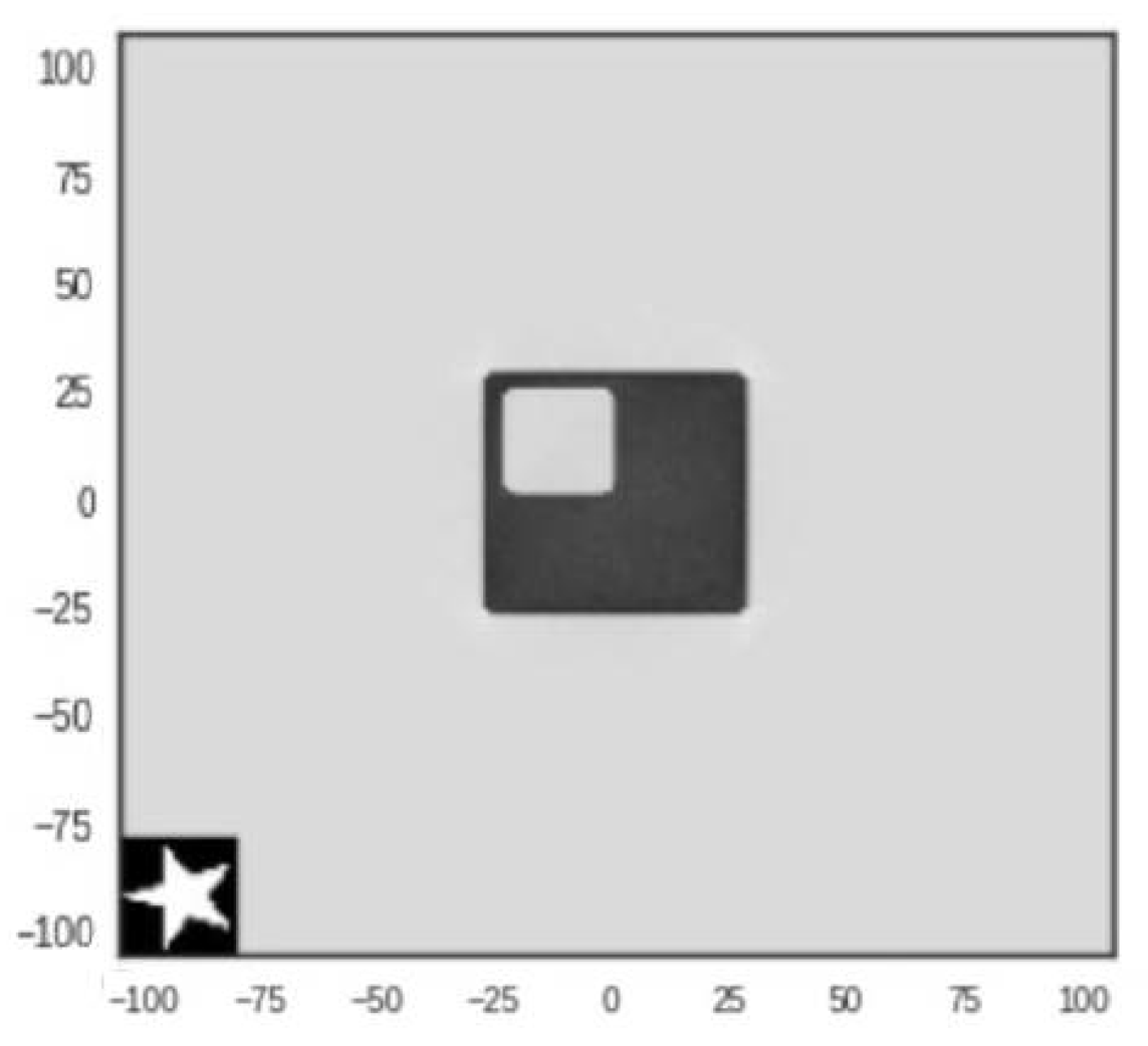
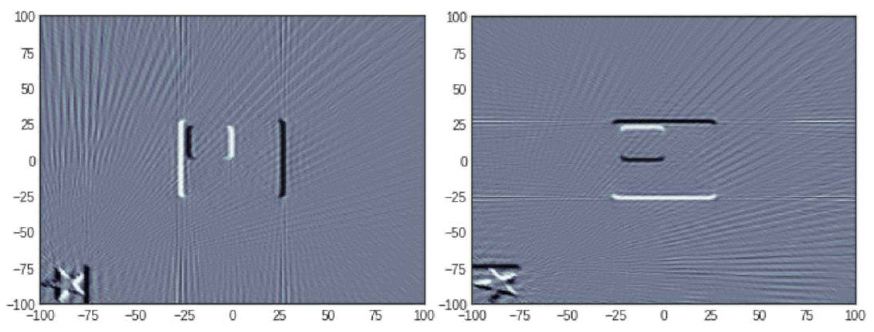
3.1. Main Idea: Planting Known Shapes in the Image

Contrarily to standard statistical approaches such as Cross-Validation and the Stein estimator of the risk, or visual quality assessment, our approach explicitly leverages the linear structure of the problem by injecting some specific information into the problem, whilst not substantially corrupting the information carried out in the observed projections. In mathematical terms, our approach consists of artificially planting a virtual shape into the image and tuning the hyperparameters so that this specific noise-free region of the image, which is known exactly beforehand, is accurately recovered. Figure 1 shows an example of a planted signal (here a star) into a cross-section image with a test sample. The test sample used was developed by the National Physical Laboratory, UK, where the sample incorporates geometries commonly seen in industrial applications. The goal of the present work is to advocate that choosing the hyperparameters so as to recover the planted shape (here, a star) accurately is a sensible approach to hyperparameter calibration.

3.2. Numerical Validation

In order to assess the relevance of using a virtual planted signal in the reconstruction scheme, we perform some numerical experiments comparing the reconstruction error on the planted signal with the reconstruction error on the total image.

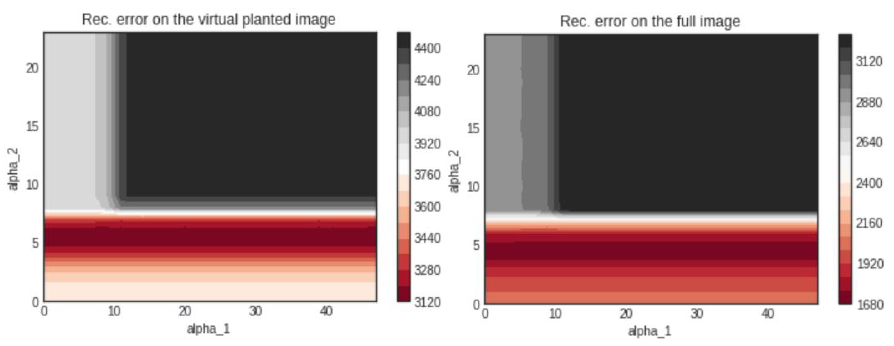
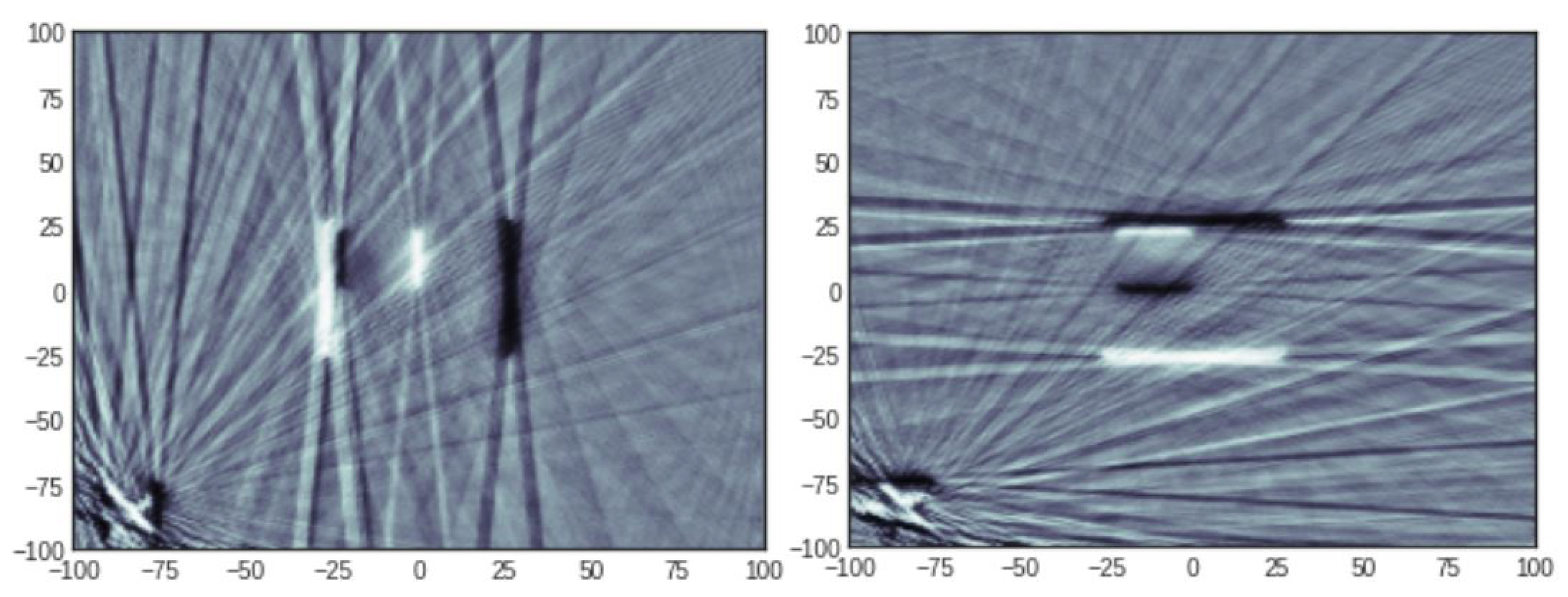
3.2.1. Comparison of the Reconstruction Errors: 20 Projections

The reconstruction error in the case of 20 projections is plotted in Figure 2. The left hand side figure shows the error landscape as a function of the two hyperparameters on the planted shape only. The right hand side figure shows the error landscape on the full unknown image.

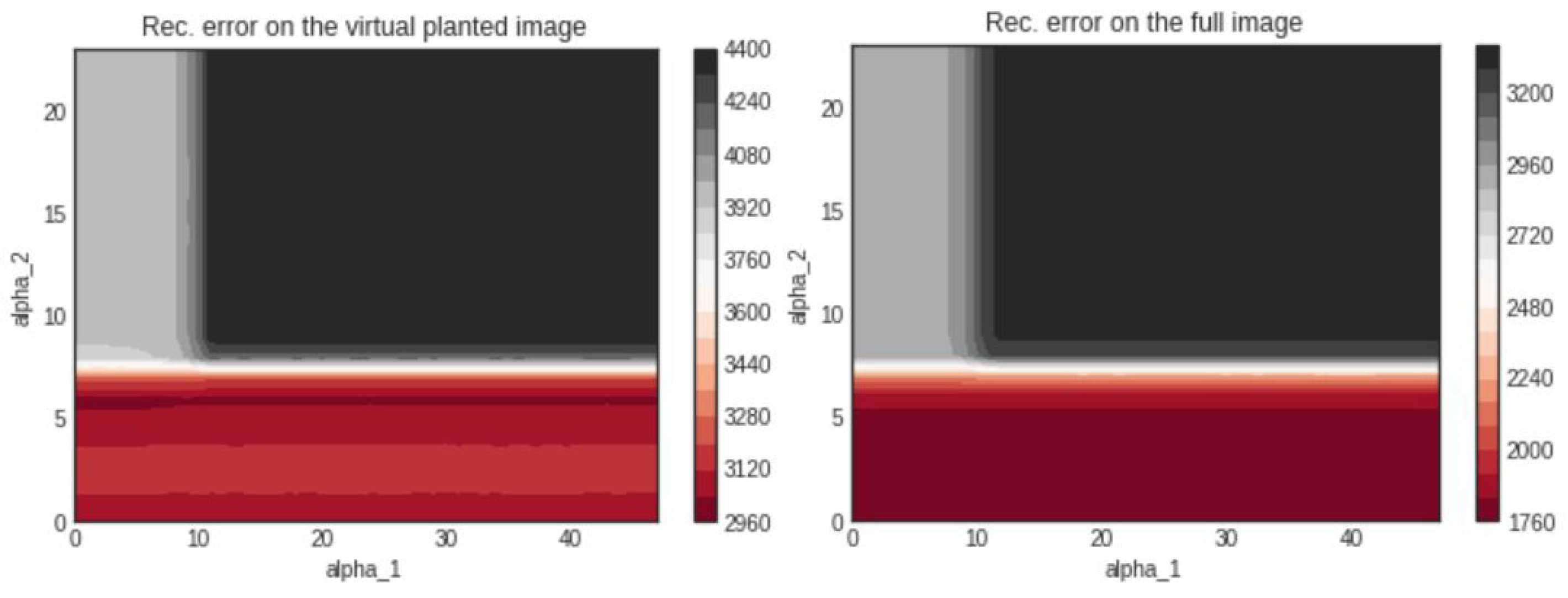
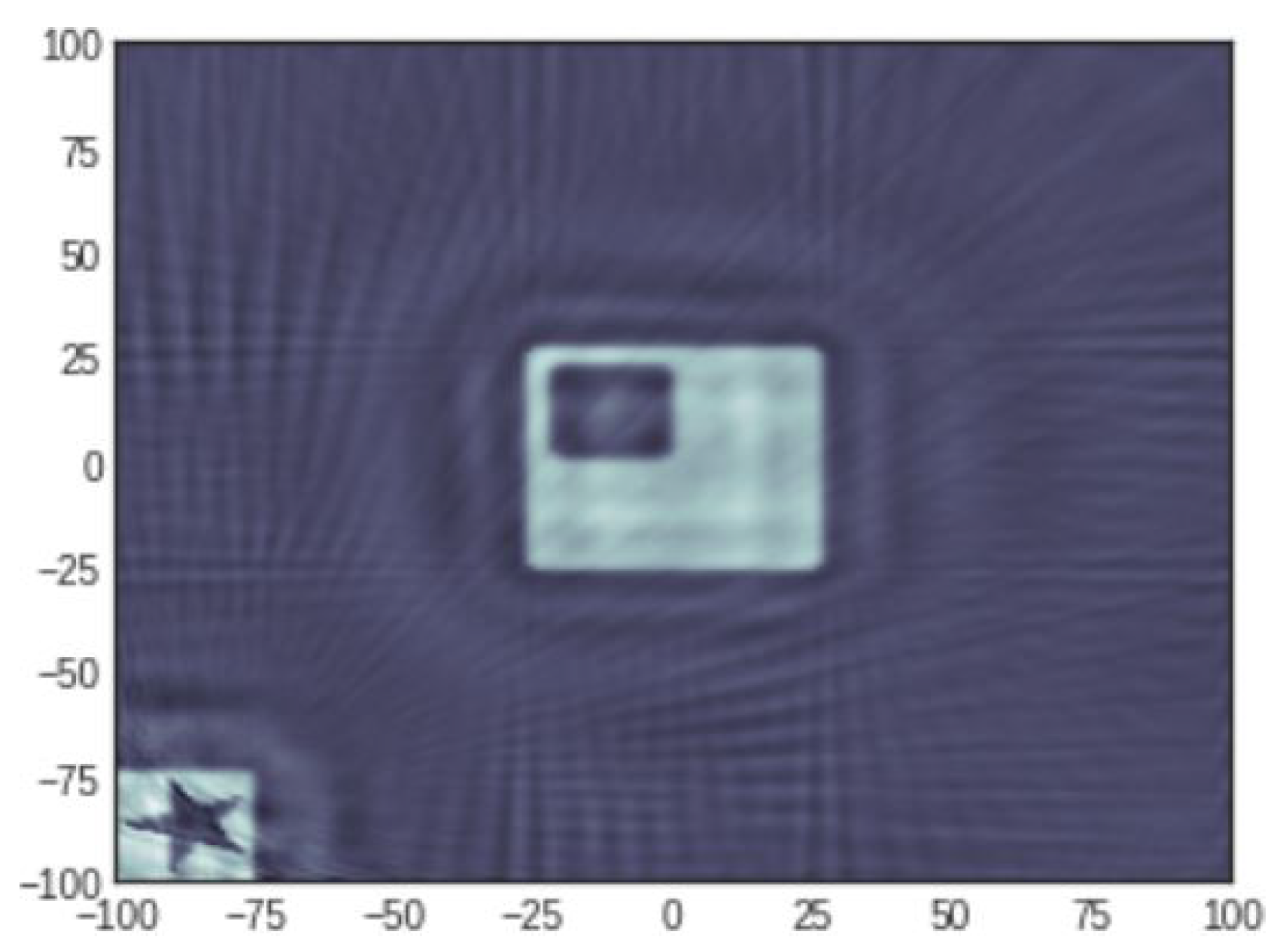
3.2.2. Comparison of the Reconstruction Errors: 50 Projections

As in the case of 20 projections in the previous section, the reconstruction error is plotted in Figure 3 for the case of 50 projections. The left hand side figure shows the error landspace as a function of the two hyperparameters on the planted shape only. The right hand side figure shows the error landscape on the full unknown image.

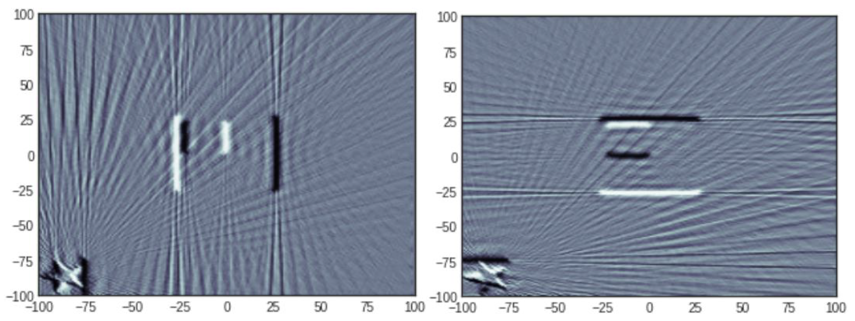
3.2.3. Comparison of the Reconstruction Errors: 100 Projections

As in the case of 20 and 50 projections in the previous section, the reconstruction error is plotted in Figure 4 for the case of 100 projections. The left hand side figure shows the error landscape as a function of the two hyperparameters on the planted shape only. The right hand side figure shows the error landscape on the full unknown image.

3.2.4. Comments on the Numerical Results

The reconstruction error as a function of the hyperparameters has not previously been studied in the literature and the error landscape shows interesting features which vary as a function of the number of projections/observations. For instance, there seems to exist an abrupt change in the reconstruction error when ${\alpha }_1$ crosses the level 37 for sufficiently small values of ${\alpha }_2$, when the number of projections is 100.

The various results obtained in the numerical experiments presented in this section show that the error landscape on the planted shape nearly faithfully reflects the error landscape on the full image. These empirical findings ensure that the proposed approach of using the reconstruction error on the virtual planted image is a relevant surrogate for tuning the hyperparameters, at least on a preliminary coarse scale. In the next section, we show how to use Bayesian Optimisation for selecting the best hyperparameters without running an exhaustive search on the 2D-grid of values of $({\alpha }_1,{\alpha }_2)$.

4. Minimising the Reconstruction Error on the Planted Virtual Image Using Bayesian Optimisation

In the previous section, we showed that the reconstruction error for the planted virtual image was a good proxy for the reconstruction error of the total image. In this section, we describe the Bayesian Optimisation framework for minimising this proxy as a function of the hyperparameters.

4.1. Description of the Method

Recently, the Bayesian optimisation approach for the model selection and tuning task has received much attention in tuning deep belief networks, Markov chain Monte Carlo methods, and convolutional neural networks; see [24]. Technically, Bayesian Optimisation relies on two main ingredients: a Bayesian statistical model for the objective function and an acquisition function for deciding where to sample next.

After evaluating the objective function according to an initial space-filling experimental design, often consisting of points chosen uniformly at random, we proceed as follows. A statistical model is chosen as a Gaussian process which provides a Bayesian posterior distribution which describes the uncertainty about the values of $f\left(x\right)$ at any candidate point x. At each iteration, we observe f at a new point and update the posterior distribution of the Gaussian process. The details of the method are given in Algorithm 1 below.

Bayesian Optimisation is a well-known technique for zeroth order optimisation. Recall that zeroth order optimisation is concerned with the problem of optimising functions in the case where we have access to its values at query points but not its gradient. In our recovery problem in particular, one can only compute the recovery error of the star signal planted in our image, but we do not have access to the gradient of this error as a function of ${\alpha }_1$ and ${\alpha }_2$. The computation of the recovery error for the planted image being expensive, Bayesian Optimisation is the tool of choice for our hyperparameter tuning problem.

Algorithm 1: Basic pseudo-code for Bayesian optimisation.

4.2. Computational Results

We now present some computational results obtained using our virtual planted image scheme combined with the Bayesian Optimisation procedure (the unit of axes of all figures plotted in this paper is in pixels).

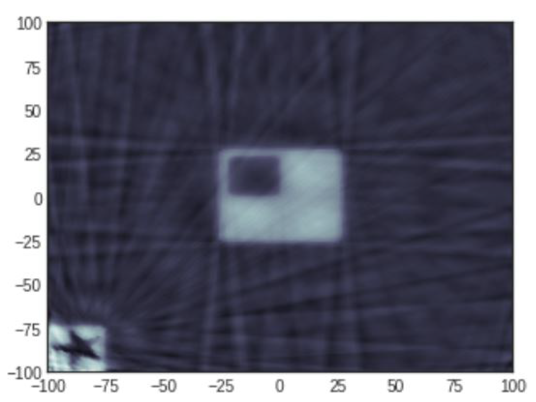
4.2.1. Reconstruction Results: 20 Projections

The optimal TGV-penalised reconstruction with 20 projections, obtained using the Bayesian optimisation approach displayed in Figure 5 and Figure 6.

4.2.2. Reconstruction Results: 50 Projections

The optical TGV-penalised reconstruction with 50 projections, obtained using the Bayesian optimisation approach and its derivatives are shown in Figure 7 and Figure 8.

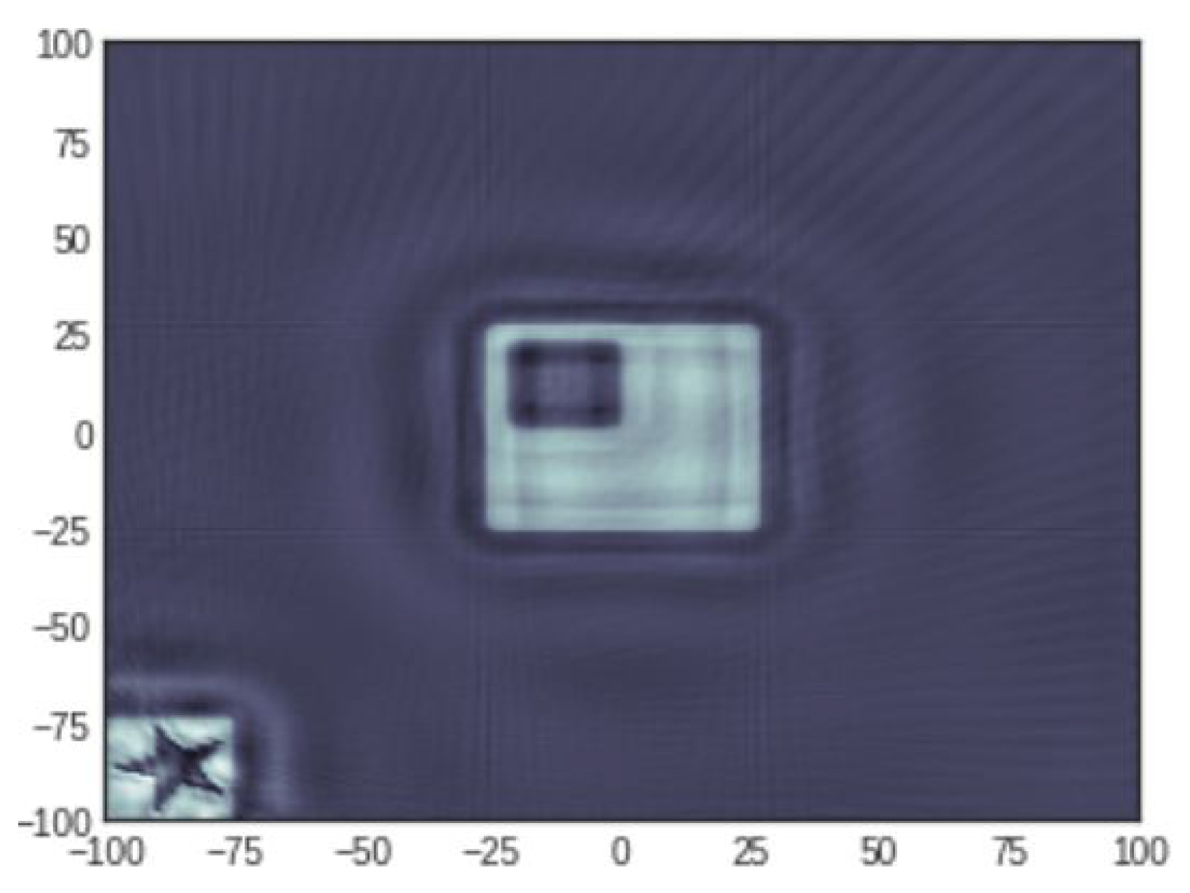
4.2.3. Reconstruction Results: 100 Projections

The optical TGV-penalised reconstruction with 100 projections, obtained using the Bayesian optimisation approach and its derivatives are shown in Figure 9 and Figure 10.

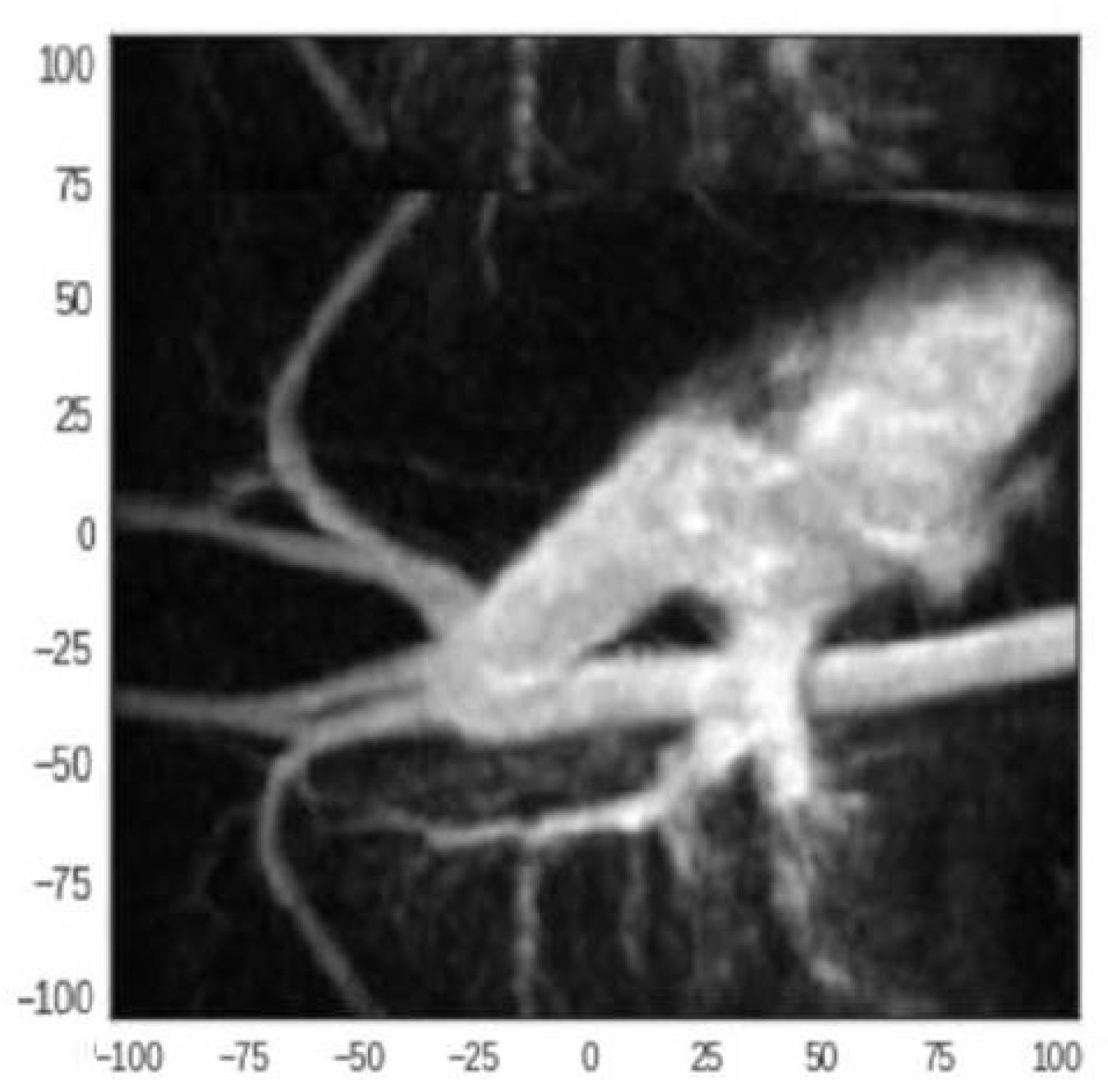
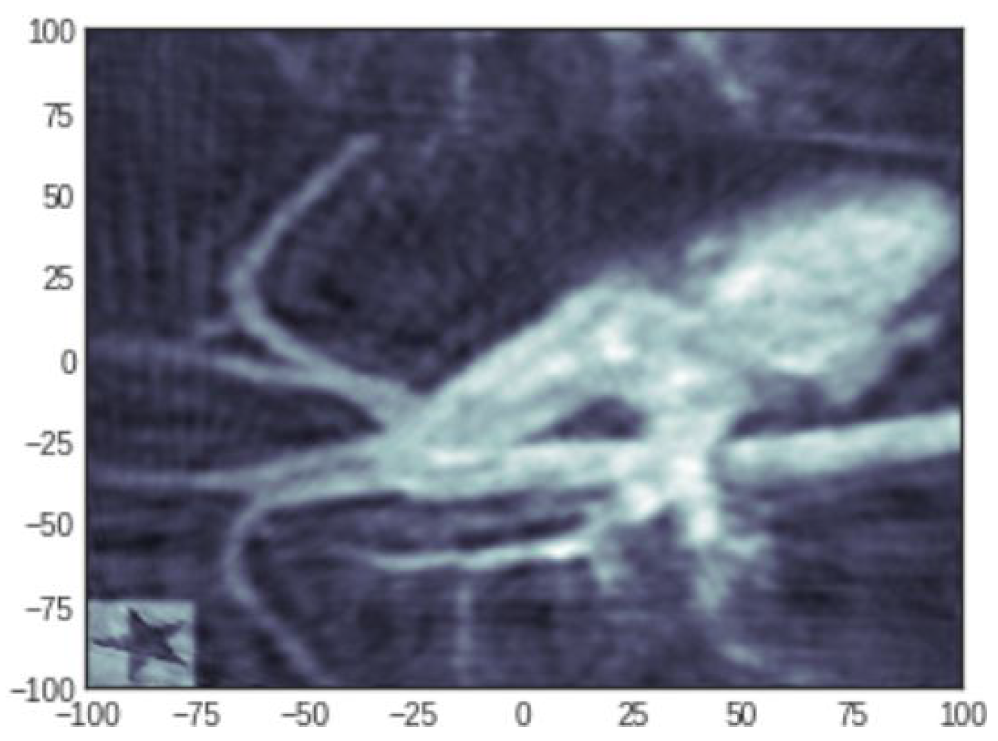
4.3. Reconstruction of a Medical Image

In this subsection, we include an example of medical image reconstruction using our approach. The original image to reconstruct is a standard aorta image from the literature shown in Figure 11.

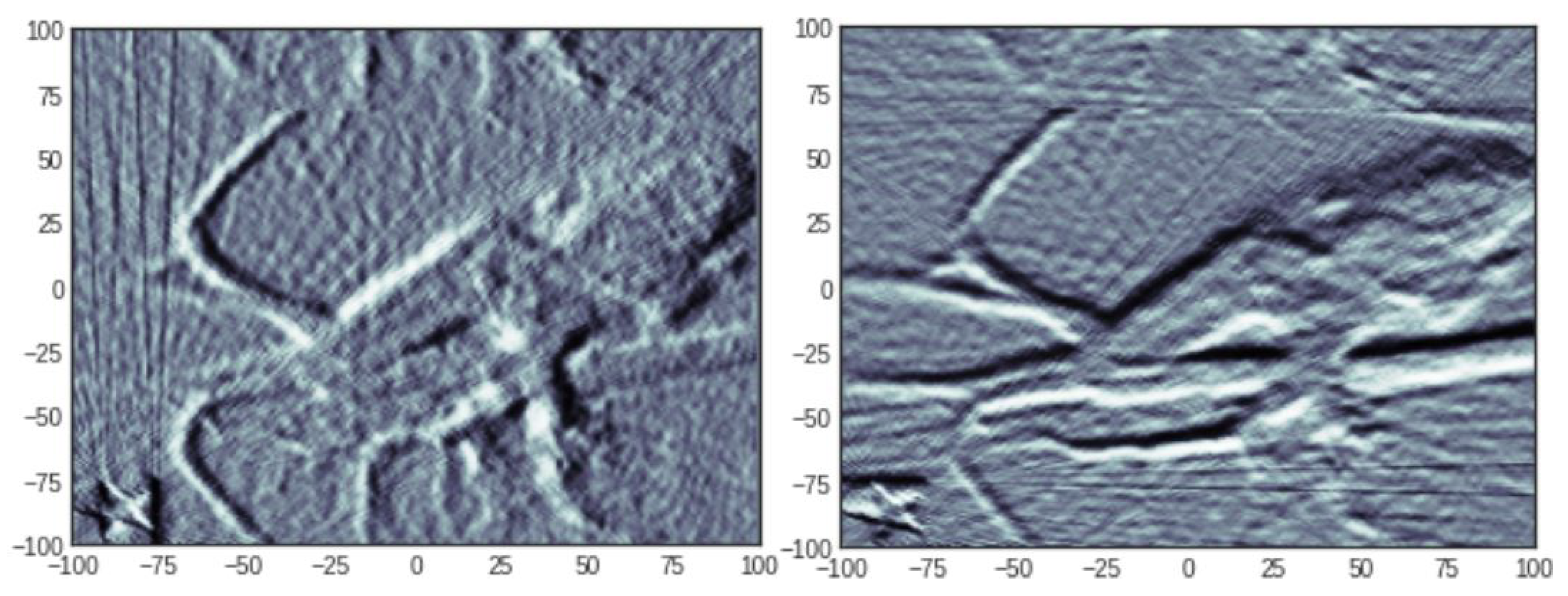
4.3.1. Reconstruction with 50 Projections

We start with an experiment using 50 projections. The reconstruction result is shown in Figure 12. The derivatives are shown in Figure 13.

These experiments confirm that our method of tuning the TGV-based reconstruction using our planted virtual image approach readily applies to this medical image reconstruction problem without changing the star shape planted image reference.

4.3.2. Reconstruction with 100 Projections

We now turn to an experiment using 100 projections. The reconstruction result is given in Figure 14. The derivatives are given in Figure 15.

The result of the TGV-based reconstruction using our planted virtual image approach is satisfactory for the case of 100 projections as well. Convergence was reached after 11 min and 47 s via Colab on CPUs.

4.3.3. Reconstruction with 100 Projections and Four Parameters

We now turn to an experiment using 100 projections but with four hyperparameters. The reconstruction result is given in Figure 16. The derivatives are given in Figure 17.

TheoOptimisation was performed within 15 min and 38 s via Colab on CPUs.

4.4. Discussion of the Benefits as Compared with the Other Approaches

We now provide the main ideas underlying the differences and potential benefits of our Bayesian optimisation approach to minimising the reconstruction error on the virtual planted image as compared with standard approaches to hyperparameter tuning.

The statistical viewpoint provides us with a rigorous framework for the hyperparameter calibration problem. As is well known, the errors incurred when hyperparameter calibration is not optimal are of two types: the bias and the variance. First, independent of the hyperparameter calibration method, penalised least-squares approaches induce an inherent bias. Debiasing is possible in some models, such as for the LASSO, as studied in [28], but it seems difficult for more general models such as obtained via TGV-based penalised least squares. In our approach, putting all our efforts into minimising the reconstruction error for the virtual planted image may induce an additional bias, which can only be mitigated if the virtual planted image is appropriately chosen. The more similar the virtual image is to the image to be reconstructed, the smaller the expected bias. If the bias induced by the choice of the virtual planted image is small, then the error committed on the virtual image is known exactly, which makes a huge difference with other statistical approaches such as Cross-Validation which can only guess the error out of strongly correlated reconstructions without ever seeing the truth. Moreover, Cross-Validation type methods work if we set a prediction task such as predicting the value of one projection given the observed values of other projections, a task which is different in a subtle manner from the actual minimisation of the reconstruction error as performed by our scheme (on a reduced area of the image). Finally, on the computational side, Bayesian Optimisation was able to find an appropriate solution at least 10 times faster than an exhaustive enumeration of all the possible combinations of the possible hyperparameter values, which is itself faster than Cross-Validation.

One of the main defects of the proposed approach is the problem of selecting an appropriate Virtual Reference Image that we superimpose to the original image to be reconstructed. Our experiments suggest that a simple surrogate such as a virtual star image can be sufficient for reaching a satisfactory reconstruction accuracy. It remains to theoretically quantify the bias incurred using our technique, a task which seems a priori quite demanding. Another possible issue we need to underline is the one of appropriately placing the virtual planted reference image into the image to be reconstructed. For this purpose, we need to know ahead of time where there should be no signal in the original image, a quite reasonable assumption in many cases. Lastly, we also would like to underline that our approach only works in the case where a linear approximation of the tomographic acquisition process is sufficiently good. In the case of a truly non-linear observation, this approach needs to be carefully extended, a task we leave for future work.

5. Conclusions

In this paper, we introduced a novel approach to efficiently calculate hyperparameters for XCT-type reconstruction problems. Our main contribution is to show that using appropriately chosen Virtual Planted Images as surrogates for the reconstruction error can help achieve satisfactory empirical performance on manufactured data at a low computational price. The approach is intuitive and very simple to implement using off-the-shelf Bayesian optimisation codes. Further studies are envisaged concerning the impact on the reconstruction error of the location of the virtual planted image in the full image to be reconstructed.

References

1. Sun, W.; Brown, S.; Leach, R. An Overview of Industrial X-ray Computed Tomography; National Physical Laboratory: Teddington, UK, 2012. [Google Scholar]
2. Candes, E.J.; Tao, T. Near-optimal signal recovery from random projections: Universal encoding strategies? IEEE Trans. Inf. Theory 2006, 52, 5406–5425. [Google Scholar] [CrossRef] [Green Version]
3. Donoho, D.L. Compressed sensing. IEEE Trans. Inf. Theory 2006, 52, 1289–1306. [Google Scholar] [CrossRef]
4. Candès, E.J. Compressive sampling. In Proceedings of the International Congress of Mathematicians, Madrid, Spain, 22–30 August 2006; pp. 1433–1452. [Google Scholar]
5. Baraniuk, R.G. Compressive sensing. IEEE Signal Process. Mag. 2007, 24, 1–9. [Google Scholar] [CrossRef]
6. Candès, E.J.; Wakin, M.B. An introduction to compressive sampling [a sensing/sampling paradigm that goes against the common knowledge in data acquisition]. IEEE Signal Process. Mag. 2008, 25, 21–30. [Google Scholar]
7. Chretien, S. An alternating l_1 approach to the compressed sensing problem. IEEE Signal Process. Lett. 2009, 17, 181–184. [Google Scholar] [CrossRef] [Green Version]
8. Giraud, C.; Huet, S.; Verzelen, N. High-dimensional regression with unknown variance. Stat. Sci. 2012, 27, 500–518. [Google Scholar] [CrossRef]
9. Chrétien, S.; Darses, S. Sparse recovery with unknown variance: A LASSO-type approach. IEEE Trans. Inf. Theory 2014, 60, 3970–3988. [Google Scholar] [CrossRef]
10. Tillmann, A.M.; Pfetsch, M.E. The computational complexity of the restricted isometry property, the nullspace property, and related concepts in compressed sensing. IEEE Trans. Inf. Theory 2013, 60, 1248–1259. [Google Scholar] [CrossRef] [Green Version]
11. Wu, T.T.; Lange, K. Coordinate descent algorithms for lasso penalized regression. Ann. Appl. Stat. 2008, 2, 224–244. [Google Scholar] [CrossRef]
12. Beck, A.; Teboulle, M. A fast iterative shrinkage-thresholding algorithm for linear inverse problems. SIAM J. Imaging Sci. 2009, 2, 183–202. [Google Scholar] [CrossRef] [Green Version]
13. Sra, S.; Nowozin, S.; Wright, S.J. Optimization for Machine Learning; MIT Press: Cambridge, MA, USA, 2012. [Google Scholar]
14. Arlot, S.; Celisse, A. A survey of cross-validation procedures for model selection. Stat. Surv. 2010, 4, 40–79. [Google Scholar] [CrossRef]
15. Assoweh, M.; Chrétien, S.; Tamadazte, B. Low tubal rank tensor recovery using the Burer-Monteiro factorisation approach. Application to optical coherence tomography. J. Appl. Comput. Math. (under review).
16. Maron, O.; Moore, A.W. Hoeffding races: Accelerating model selection search for classification and function approximation. In Advances in Neural Information Processing Systems; Carnegie Mellon University: Pittsburgh, PA, USA, 1994; pp. 59–66. [Google Scholar]
17. Chretien, S.; Gibberd, A.; Roy, S. Hedging parameter selection for basis pursuit. arXiv 2018, arXiv:1805.01870. [Google Scholar]
18. Li, L.; Jamieson, K.; DeSalvo, G.; Rostamizadeh, A.; Talwalkar, A. Hyperband: A novel bandit-based approach to hyperparameter optimization. J. Mach. Learn. Res. 2017, 18, 6765–6816. [Google Scholar]
19. Donoho, D.L.; Johnstone, I.M. Adapting to unknown smoothness via wavelet shrinkage. J. Am. Stat. Assoc. 1995, 90, 1200–1224. [Google Scholar] [CrossRef]
20. Stein, C.M. Estimation of the mean of a multivariate normal distribution. Ann. Stat. 1981, 9, 1135–1151. [Google Scholar] [CrossRef]
21. Zou, H.; Hastie, T.; Tibshirani, R. On the “degrees of freedom” of the lasso. Ann. Stat. 2007, 35, 2173–2192. [Google Scholar] [CrossRef]
22. Snoek, J.; Larochelle, H.; Adams, R.P. Practical bayesian optimization of machine learning algorithms. In Advances in Neural Information Processing Systems; NeurIPS: Toronto, ON, Canada, 2012; Volume 25. [Google Scholar]
23. Eggensperger, K.; Feurer, M.; Hutter, F.; Bergstra, J.; Snoek, J.; Hoos, H.; Leyton-Brown, K. Towards an empirical foundation for assessing bayesian optimization of hyperparameters. In Proceedings of the NIPS workshop on Bayesian Optimization in Theory and Practice, SEMANTIC SCHOLAR, Lake Tahoe, NV, USA, 5–8 December 2013; Volume 10. [Google Scholar]
24. Shahriari, B.; Swersky, K.; Wang, Z.; Adams, R.P.; De Freitas, N. Taking the human out of the loop: A review of Bayesian optimization. Proc. IEEE 2015, 104, 148–175. [Google Scholar] [CrossRef] [Green Version]
25. Wu, J.; Chen, X.Y.; Zhang, H.; Xiong, L.D.; Lei, H.; Deng, S.H. Hyperparameter optimization for machine learning models based on Bayesian optimization. J. Electron. Sci. Technol. 2019, 17, 26–40. [Google Scholar]
26. MacKay, M.; Vicol, P.; Lorraine, J.; Duvenaud, D.; Grosse, R. Self-tuning networks: Bilevel optimization of hyperparameters using structured best-response functions. arXiv 2019, arXiv:1903.03088. [Google Scholar]
27. Bredies, K.; Kunisch, K.; Pock, T. Total generalized variation. SIAM J. Imaging Sci. 2010, 3, 492–526. [Google Scholar] [CrossRef]
28. Zhang, C.H.; Zhang, S.S. Confidence intervals for low dimensional parameters in high dimensional linear models. J. R. Stat. Soc. Ser. B Stat. Methodol. 2014, 76, 217–242. [Google Scholar] [CrossRef] [Green Version]
Figure 1. An example of a planted signal (here a star). The test sample used was developed by the National Physical Laboratory, UK, where the sample incorporates common geometries seen in industrial applications.The unit of axes is in pixels.
Mathematics 09 02960 g001
Figure 2. Reconstruction error as a function of the hyperparameters α 1 and α 2 from (7): planted star error (left) and full image (right).
Mathematics 09 02960 g002
Figure 3. Reconstruction error as a function of the hyperparameters α 1 and α 2 from (7): planted star error (left) and full image (right).
Mathematics 09 02960 g003
Figure 4. Reconstruction error as a function of the hyperparameters α 1 and α 2 from (7): planted star error (left) and full image (right).
Mathematics 09 02960 g004
Figure 5. Reconstruction based on 20 projections, with a planted star in a void area of the object used to calibrate the hyperparameters. The unit of axes is in pixels.
Mathematics 09 02960 g005
Figure 6. Derivatives in x and y of the reconstructed image shown in Figure 5.
Mathematics 09 02960 g006
Figure 7. Reconstruction based on 50 projections, with a planted star in a void area of the object used to calibrate the hyperparameters. The unit of axes is in pixels.
Mathematics 09 02960 g007
Figure 8. Derivatives in x and y of the reconstructed image shown in Figure 7.
Mathematics 09 02960 g008
Figure 9. Reconstruction based on 100 projections, with a planted star in a void area of the object used to calibrate the hyperparameters. The unit of axes is in pixels.
Mathematics 09 02960 g009
Figure 10. Derivatives in x and y of the reconstructed image shown in Figure 9.
Mathematics 09 02960 g010
Figure 11. Original aorta image.
Mathematics 09 02960 g011
Figure 12. Reconstructed image based on 50 projections.
Mathematics 09 02960 g012
Figure 13. Derivatives in x and y of the reconstructed aorta image.
Mathematics 09 02960 g013
Figure 14. Reconstructed image based on 100 projections.
Mathematics 09 02960 g014
Figure 15. Derivatives in x and y of the reconstructed aorta image.
Mathematics 09 02960 g015
Figure 16. Reconstructed image based on 100 projections.
Mathematics 09 02960 g016
Figure 17. Derivatives in x and y of the reconstructed aorta image.
Mathematics 09 02960 g017
Publisher’s Note: MDPI stays neutral with regard to jurisdictional claims in published maps and institutional affiliations.