
Parallel Algorithms for Solving Inverse Gravimetry Problems: Application for Earth’s Crust Density Models Creation


Bulashevich Institute of Geophysics, Ural Branch of Russian Academy of Science, Amundsena 100-305, 620016 Ekaterinburg, Russia
*
Author to whom correspondence should be addressed.
Mathematics 2021, 9(22), 2966; https://0-doi-org.brum.beds.ac.uk/10.3390/math9222966
Submission received: 21 October 2021
/
Revised: 19 November 2021
/
Accepted: 19 November 2021
/
Published: 20 November 2021
(This article belongs to the Special Issue Numerical Analysis and Scientific Computing)
Abstract
:The paper describes a method of gravity data inversion, which is based on parallel algorithms. The choice of the density model of the initial approximation and the set on which the solution is sought guarantees the stability of the algorithms. We offer a new upward and downward continuation algorithm for separating the effects of shallow and deep sources. Using separated field of layers, the density distribution is restored in a form of 3D grid. We use the iterative parallel algorithms for the downward continuation and restoration of the density values (by solving the inverse linear gravity problem). The algorithms are based on the ideas of local minimization; they do not require a nonlinear minimization; they are easier to implement and have better stability. We also suggest an optimization of the gravity field calculation, which speeds up the inversion. A practical example of interpretation is presented for the gravity data of the Urals region, Russia.
1. Introduction
Gravity data inversion is the main tool for obtaining the Earth’s crust density model. Our main goal of the study is to construct a stable high-resolution method of three-dimensional (3D) gravity data inversion. The simplest approach of finding 3D density values is by forward gravity modeling. We can vary the initial model in an interactive mode to reduce the gravity field residuals. However, such an approach cannot resolve the non-uniqueness and instability of inverse problem solving. Our method of inversion follows the procedure of Cordell and Henderson [1]. The density values are calculated using the observed gravity field by iterative regularized algorithm, without the time-consuming trial-and-error procedure.
The interpretation process involves solving the forward and inverse gravity problems. The inverse gravity problems are ill-posed since their solution is non-unique and unstable depending on the initial data [2], hence why one should define the set of correctness for the solution and select a reasonable initial condition. Density is one of the most important parameters for geophysical modelling. Density models are usually created using complete information (for example, seismic data) to select the initial model. We apply the iterative scheme for transforming the model slightly at each step to create the geological meaningful density model [3]. To extend the layer outside the study volume, we suggest selecting piecewise-constant density function , which depends only on depth.
We propose a method for constructing density models with flat topography based on inversion of gravity data with a complete Bouguer correction. In this article we describe the creation of a density model method for layered medium. The process of constructing density models based on gravity field anomalies proposed here contains five major steps: the fast forward modeling algorithm; the initial 3D density model creation; the upward and downward continuation (the extraction of the gravity fields of layers); the choice of the density as multiplicative function; and the stable adaptive algorithm for the inverse problem solving. The horizontal layered models may well correspond to reality in some areas but deviate from the actual geology in others; this is a limitation of the method.
For layer-by-layer separation of the gravitational field by depth, we use a filter based on the analytical continuation of the vertical field component upward and downward with Lavrentiev’s regularization. Several researchers have been engaged in the downward continuation of potential fields. In [4], the authors apply Tikhonov’s regularization to stabilize the process of solving this problem. They present realization of the method in the form of a Matlab-based program. The optimum regularization parameter value is selected as a local minimum of constructed Lp-norms functions-in the majority of cases. They demonstrate excellent stabilizing properties of this method on several synthetic models and one real-world example from high-definition magnetometry.
In [5], the authors propose using the combination of upward continuation and horizontal derivative to accomplish the downward continuation of potential field data. The proposed method was demonstrated on synthetic potential field data. The method was also applied to real potential field data, and the results show that the proposed method accomplishes the downward continuation of the real data, stably.
An alternative method of downward continuation is proposed in [6]. The authors use a combination of Taylor series expansion and upward continuation for computing vertical derivatives. This method has been tested on the gravitational anomaly of infinite horizontal cylinder in both cases with and without random noise. The vertical derivative method is applied to calculate the downward continuation according to the Taylor series expansion method. The method was also tested on both complex synthetic models and real data.
In [7], the authors formulate a functional model for a spectral downward continuation of selected gravitational field quantities to an irregular topographic surface. This functional model is further generalized to allow for transformation between different types of gravitational field quantities. In particular, spectral weights are derived for estimation of the disturbing potential or disturbing/anomalous gravity at the Earth’s surface by combining the first-, second- and third-order radial gradients of the disturbing potential (disturbing gradients). The combined spectral estimator is applied to simulated satellite disturbing gradients polluted by a realistic Gaussian noise. The spectral combination method requires no matrix inversion.
Another example of applying regularization to inversion of potential field data is presented in [8]. Authors have introduced a new processing and modeling technique of magnetic data conducted over mines or near-surface geophysical targets for accurate and precise determination of location and depth. The technique is based on the application of the Kaczmarz regularization method to the ill-posed magnetic inverse problem. The advantage of this method is the optimum transformation of regularized normal equations to an equivalent augmented regularized normal system of equations. The method is applied to an unexploded ordnance test site in the United Kingdom.
A fast algorithm for a forward gravity problem is absolutely essential for efficiently solving the inverse problem. We build the initial density model using deep seismic sounding (DSS) data along two-dimensional seismic profiles. The volume between profiles is filled with interpolated values of density on a regular 3D grid [3]. Each cell of the grid is a rectangular prism with constant density. The analytical form for the gravity field of the rectangular prism is well-known [9,10]. The finite element method (FEM) in forward modelling is used in this study. Mostafa [11] and Couder-Castañeda et al. [12] are relevant studies that consider relatively small grid sizes: the models consist of 10,000–15,000 prisms in each example. For our study, we required a technique that could handle more than a billion elements in a reasonable time. Therefore, we cannot rely on parallelization alone and it is necessary to modify the algorithm itself. We note that Dubey and Tiwari [13], Li and Oldenburg [14] consider elements of non-equal size, and affirm that FEM can also be applied in iterative field inversion.
The correctness of the 3D inversion depends on the technique of mass continuation outside the study area. One cannot simply consider that density is zero everywhere outside. In this paper, the authors use background density, calculated by averaging the density values of every horizontal layer of the interpolated model. This approach is similar to that presented by Cai and Wang [15].
The paper is organized as follows: we present new mathematical algorithms for downward continuation of the gravity field and the 3D inverse problem, and then both algorithms are applied to the gravity anomalies of the Middle Urals region, Russia.
2. Methods
2.1. Layer-by-Layer Separation of the Local Field Component
In [16], a technique was proposed for separating the sources of the gravitational field by depth. Examples of the implementation of the technique are given in and [17]. In this paper, we describe an implementation of this technique based on a new and more efficient numerical algorithm that enables parallel computing on graphics accelerators.
In order to separate the observed field anomalies by depth, we use the original method of elevated transformations [16,18] with the modification of the computational part, proposed by the authors of this paper, based on the method of local corrections [17,19,20]. We use this method for downward continuation and the density refinement. We assume that the original field is specified on the plane z = 0.
The general scheme of the method for isolating the effects of the sources in a layer down to the certain depth (concerning the Earth’s surface) z = −H consists of three stages.
- 1.
- We construct the analytical continuation of the field upward to the height z = H: , while assuming that the influence of the local near-surface sources (down to the depth z = −H) is significantly weakened or eliminated at all.
- 2.
- In order to hide the influence of the local sources located in the horizontal layer between the plain z = 0 and the plain z = −H, the field is recalculated upwards is then analytically continued downward to the depth z = −H: . Moreover, since the problem is ill-posed, it is necessary to use methods with regularization, hence κ in the formula is a regularization parameter. The resulting field is calculated on the plane z = −H from sources located below the boundary z = −H.
- 3.
- At the last step, we recalculate the field upward again to the level of the plain z = 0: . The resulting field is calculated on the plane z = −H from sources located below the boundary z = 0. Further, we subtract this field from the original one obtaining the field for the layer : .
If we want to obtain the field on the plane z = 0 from the sources located in the depth interval , then we must perform three stages of the method for the heights H1 and H2, and then take the difference between the results: .
Thus, if the observed field g (x, y, 0) is given on the plane z = 0, and there is also an ordered set of depths , , then the problem of dividing g(x, y, 0) into components on the plane z = 0, corresponding to fields from sources located in depth intervals , can be solved as follows. For every depth independently, the three steps of the recalculation method described above are performed, and the field is obtained. In this case, at the second stage, the regularization parameter is used, Further, the difference for the successive depths is calculated . It turns out that .
2.2. Definition of the Operation Up(·)
Suppose the gravitating masses are located in the layer below the horizontal plane at the depth z. On this plane, we denote the gravitational field by and consider it as the boundary function for the Dirichlet problem for the Laplace equation over a semi-infinite domain. From the values on the boundary, the solution reconstructs the harmonic field function everywhere above z. So, for the upper half-space the solution of the problem can be written in terms of the Poisson integral [21]:
The operation of the upward recalculation is a direct calculation of the integral in the Formula (1). The operation of the downward recalculation is the solution of the Fredholm integral equation of the first kind (1), where the values of the field are assumed to be given, and the values of under the integral sign are to solve for. In the general case, finding a solution to this equation is an ill-posed problem requiring regularization, which is, again, reflected in the notation: κ is the regularization parameter.
The implementation of the operation for the upward recalculation that accounts for the difference in heights , described in detail here, will be used later in the paper. We assume that the field u(x,y,z) is defined everywhere on the z plane as a piecewise constant function:
where , , can be considered as the horizontal asymptote of the field. In this case, the integral (1) is obtained analytically in the following form:
where .
The field asymptote does not change during recalculation. Formula (3) allows for calculating the values of the field recalculated to the height ζ at the point. For the downward recalculation we must approximate the upward recalculated field by a piecewise constant function at the same intervals as the field . To do this, we need to average over the said intervals:
where , .
Note that in the sequential calculation for all possible indices and according to the Formula (5), we would have to compute the value of the ν function times. However, it is possible to reduce this number if we assume that the field sampling grid is uniform in x and y, then and we can rewrite (5) as:
Applying the same optimization technique for calculating the convolution of functions on a uniform grid, which was used in [20], for a fast algorithm for solving the forward gravity problem, we can write (7) in the form:
where , suppose that , if ; .
Thus, recalculation consists of following steps.
- The preprocessing stage. This stage is done once and is suitable for any initial field, depends only on the difference in the heights H of the recalculation and the grid discretization steps Δx, Δy. It is based on the fact that the elements do not depend on the input amplitudes of the field, only on H, Δx, and Δy. The stage consists of calculating elements of the set . Note that the function is even for x and y and odd for z, hence , so in fact, one only needs to calculate values of for different arguments, which is an order less than values when calculating “directly” as per (5).
- Setup initial data: set from elements (field amplitudes in piecewise constant representation).
- 1.
- Calculation of elements of the set .
- 2.
- Calculation of elements of the set (8).
- 3.
- Calculation of elements of the output set (6).
As one can see, the preprocessing step, which is lengthy in terms of the computation time, is not directly included in the recalculation up(H) at all (steps 1–3). This fact makes it possible to significantly reduce the calculation time of the downward recalculation operation down(H,), which is defined later.
Similar to (8), one can write the “fast” version of (3) for the upward recalculation for a set of points of the form :
where . Moreover, if and are fixed, ,, then the value of the arctangent must be computed for different arguments. If, under the same conditions, we use Formula (3), then we would need of arctangent computations. As it becomes evident, among these values there would be no more than unique ones, which was not completely evident from the expression (3).
2.3. Description of the Operation Down(·,·)
The implementation of the down(H, κ) operation for downward recalculation for the height difference , with a regularization parameter κ, is described in detail hereAs mentioned above, it is necessary to solve the Fredholm integral equation of the first kind (1) for the unknown function , where z is fixed.
We will use the same piecewise constant function representation of the field as its parameterization as for the operation up(H), we seek in the form of (2) and assume that the field on the left side of (1) is given by its mean values (4) within the indicated boundaries. We seek using the modified method of local corrections, which was described as a solution of linear inverse gravimetry problem in [20]. Its stages for solving Equation (1) with the chosen parameterization are reproduced as follows. The initial data at the iteration “zero” (the iteration number is denoted by the superscript in parentheses): the set of the “residual” field amplitudes at a height ζ (we take ); the set of the field amplitudes at height z (we take ). The definition of the “residual” field is at the iteration θ: assuming that , then . At each iteration the horizontal asymptote for all fields appearing in the algorithm remains equal . Notice that it is not the absolute values of the fields that are important, but their deviations from the asymptote. To explain the used notation: when we write , , , , we mean the average value of these functions in the region , when we write , , , , (without indices) we mean piecewise constant functions depending on x and y in the domain . For the method below, it is essential that the region in x and y, on which we will vary the required function , is and coincides with the region of the actual definition of the known field at the height ζ. Moreover, the values of all functions , , , , appearing in the method that are outside of the region are set to the value of the horizontal asymptote . For example, the results of up(H) recalculation outside the specified region are replaced with .
So, the stages of the modified method of local corrections for solving (1) with the chosen piecewise constant parameterization are as follows:
- 1.
- Calculate operation up(·) for . On a side note, according to the physical meaning of the up(H) recalculation, the field is defined in the plane with the applicate ζ + H. But in what follows, we only need as a formal function of x and y, its physical meaning is of no matter.
- 2.
- Calculate and :where for the selected parameterization will be written in the form ; S is upward recalculation for the difference in heights H of the unit field which is equal to if or if
- 3.
- Calculate .
- 4.
- As we can see, hence we calculate .
- 5.
- Evaluate termination criteria: (reaching the required accuracy ε of the field approximation).
If the expressions (6, 8) are used in the algorithm above at stage 1 to recalculate upwards, then the approximated value will denote the average of the field over the regions , which should be obtained as a result of upward recalculation of the required field . If, at the first stage, we use the expression (9) with the condition , then the values will denote the values of the recalculated field at the specific points of the form . Both options can be used, but it is worth noting that the iterative process will be more stable if we use the average over the region instead of the value at just one point in that region. Also, in the second case is the value of at one specific point in the region . For the operation up(H) in the chosen piecewise constant parameterization, it is required to “continue” over the entire region, which introduces more error than the “fair” averaging. In addition, the formula for the dot product given in step 2 yields better result with averaging.
As our experiments show the above method converges even without classical regularization (in both versions: with averaging and “pointwise”), but, perhaps, will not reach zero error ε. However, for the purposes described in the next section, we introduce a formal regularization. Since the kernel of the integral (1) is symmetric and positive definite, we can apply Lavrentiev’s regularization [22]. The regularized equation is:
where and are fixed, is regularization parameter. This equation has exactly one solution in for any left side function in . The solution depends continuously on [22]. The Equation (10) can be solved by the modified method of local corrections proposed earlier for Equation (1) with piecewise constant parameterization, but requires a modified method of calculating on the first step: instead of should be , .
2.4. Applying the Recalculations to Recover the Density Model
We consider the proposed method for separating the gravitational effect of sources from the total observed field in the half-space below certain depth : . Let be specified exactly by its piecewise constant representation. If the operations up(H) and down(H,0) were performed precisely, in the analytical form, then the result would be . In the proposed recalculations, however, there are inaccuracies: the averaging of the exact results of up(H) in the cells and equating the values up(H) and down(H,0) to horizontal asymptote outside the target region .
The authors have carried out a large number of numerical experiments with the data of the real measured fields. In the worst cases of “high-frequency” fields and large H (of the order of 100 km), the residual was not more than 10% and not more than 1% for H < 40 km. So, if we strive for the greatest accuracy when implementing the recalculation scheme using the analytic continuation of harmonic functions, then the separation of the fields will not work. Actually, for the purposes of separation, the formal regularization was introduced into the operation down(H,κ).
The result of the three-stage recalculation scheme continuously depends on the regularization parameter κ. We separate the observed field along L horizontal layers with depth intervals and consider is the field of this layer, while the fields are obtained using the regularization parameters , with the exception of , , . If we assume that the entire observed field is generated by the masses in the layer , then it is necessary to ensure , for this should large enough. To fulfill the condition of “continuous” joining of the separated fields of adjacent layers, it is required to choose in ascending order between and without abrupt transitions from to . Increasing with depth produces a sequence of separated fields in accordance with the physical meaning: the deeper layers are more “smoothed”. Of course, there are infinitely many options for “continuously” increasing sequence of , and different options can give significantly different recalculations and, accordingly, different density models. This is precisely where the non-uniqueness of the solution to the linear inverse gravimetry problem is manifested. Here, the choice falls on the shoulders of the interpreter and is subjective. One helpful fact is that small changes in the sequence of will lead to small changes in the separated fields and the resulting density model.
Thus, κ is used in recalculations not for regularization really, but as a continuous smoothing factor, which cannot be replaced by, for example, several passes through the observed field with a discrete Gaussian filter in the “time” domain, because even one such path for the upper layers is too many. Frequency domain filters can also be used for the purpose of separating fields, but it seems they are less justified in terms of binding to the specific depths.
2.5. Inverse Gravity Problem for the Layered Medium Model
Calculations of the 3D density distribution in an inhomogeneous region D based on field values are implemented by inversion of integral operator [21] on the right hand side of (11), where g is a known function, γ is the gravitational constant.
Mathematically, this is an ill-posed problem and its solution depends drastically on small variations in the initial field data g. However, if we select a density class with only lateral density variations, the determination of the density distribution in the horizontal layer will be stable [23]. Let be the rectangular prism filled with mass and be the observed gravity field separated for the layer using described above recalculation technique. Weseek the density in the form of , where is the density of initial model and it is assumed to be known. Further, we assume may be approximated by some kind of the initial model analysis.
The 2D function is defined based on the Fredholm integral equation:
where
where is the field of the initial model.
The numerical solution of the Equation (12) is based on the local corrections method [20]. This approach allows one to solve the problem without usage of non-linear minimization and, thus, reduce the calculation time. Iterative algorithm for the refinement values of minimizes the discrepancy of the observed and model fields. First, the field of the initial model is calculated. Thus, the residual field is . We assume that , , , .
The following steps are repeated in a loop (for the iterations θ ≥ 1).
- 1.
- Calculate
- 2.
- Determine and :
- 3.
- Calculate
- 4
- Calculate
- 5.
- Evaluate termination criteria: (achieving the required accuracy ε of the field approximation).
Once the loop is complete, the excess density distribution approximates (up to a constant) the difference between the observed and initial model fields. After summing the initial model with obtained distribution, we obtain the density model with the field that differs from the observed one by the amount of error of .
The described algorithm relies on the solution of the forward problem only (step 1). The lateral density is calculated using the difference between the observed field and the model field at each iteration step. For this reason, no classical regularization (in Tikhonov sense) is required. One can regulate convergence of the iterative process by coefficients and . Thus, the problem of calculation of corrective additive could be solved independently for all layers. Therefore, the uniqueness of the solution to the equation of the inverse problem for the lateral density [23] and the whole problem is guaranteed.
3. Experimental Results. Three-Dimensional Density Model of Middle-Urals Region
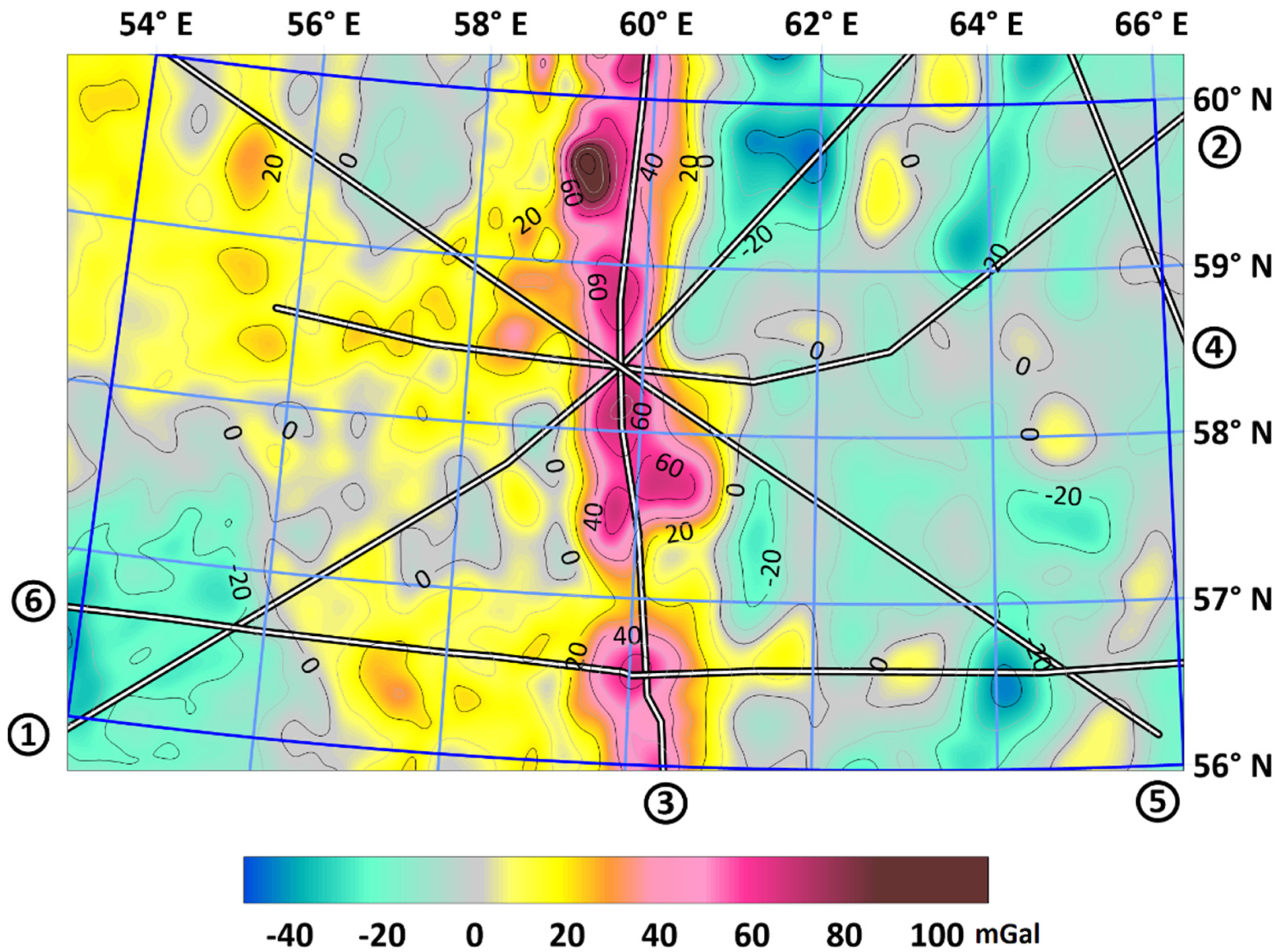
In this section, we demonstrate the described method on the case study of Middle-Urals, Russia, and neighboring regions. The territory is located at 56–60° N and 54–66° E, the model thickness is 80 km down from the Earth’s surface level. The given gravity field with a complete Bouguer correction (the combined global gravity field model XGM2019e_2159 [24]) is presented in Figure 1. The position of DSS profiles is drawn as black and white lines. The maximum depth of the profile sections is 80 km [25].
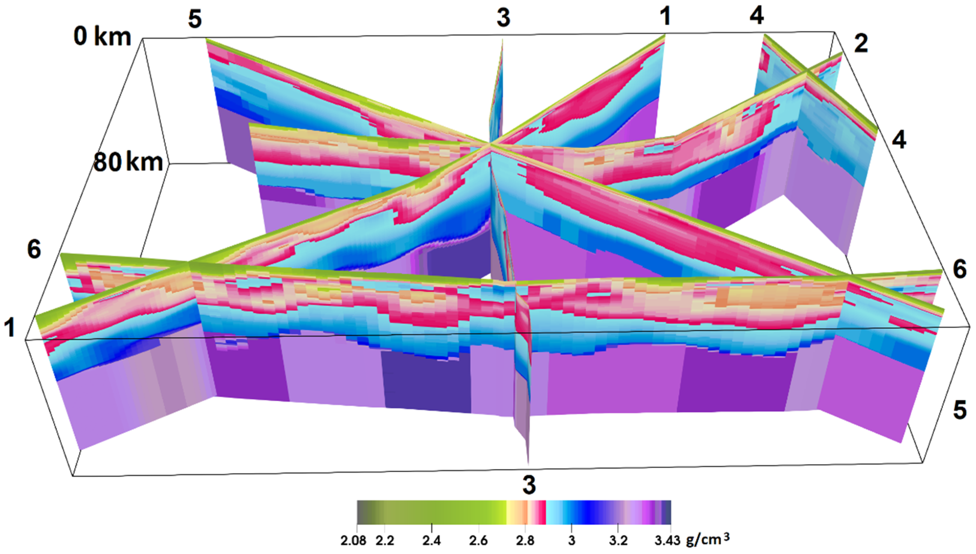
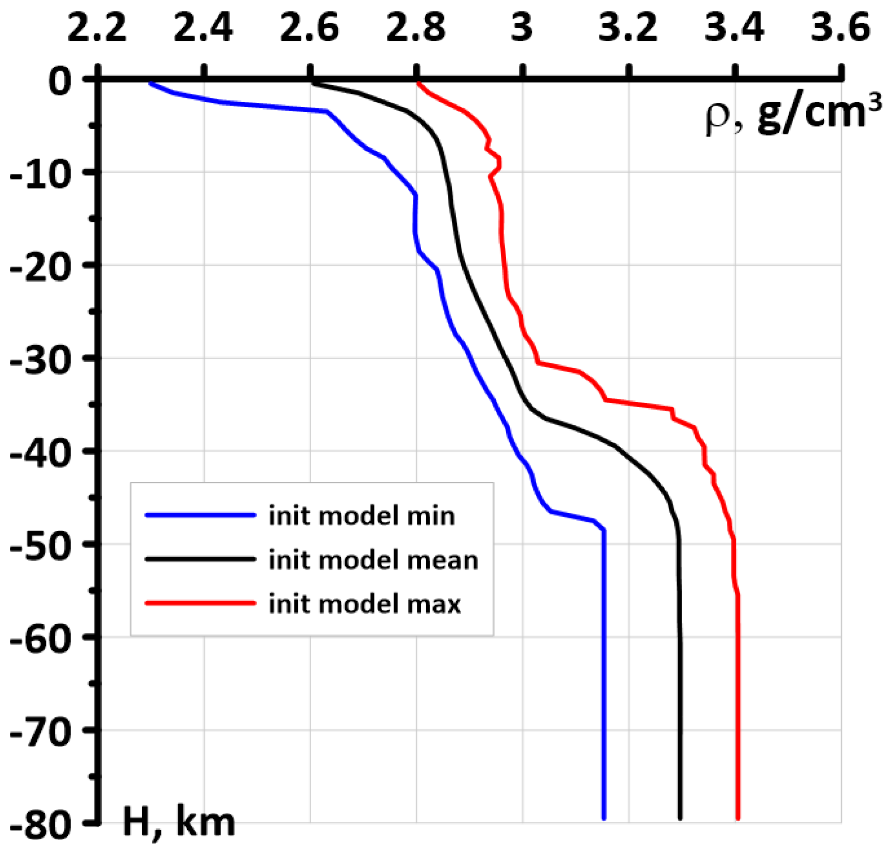
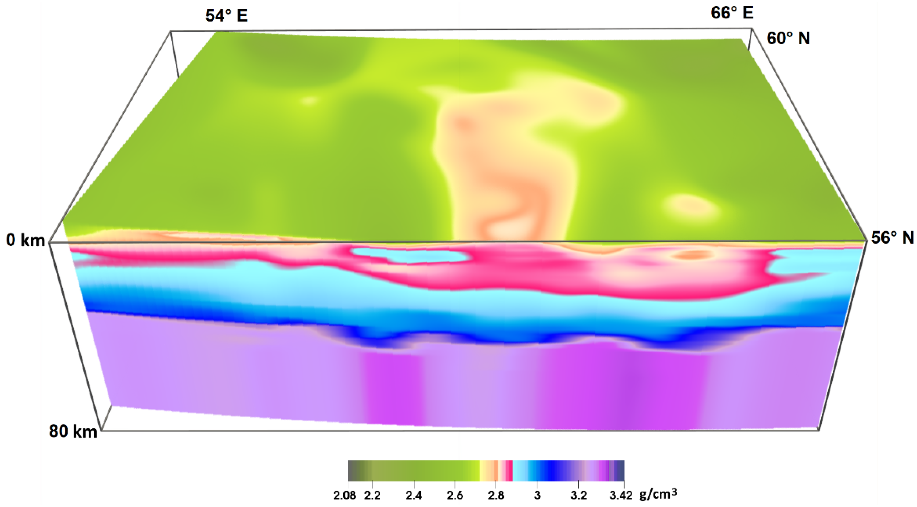
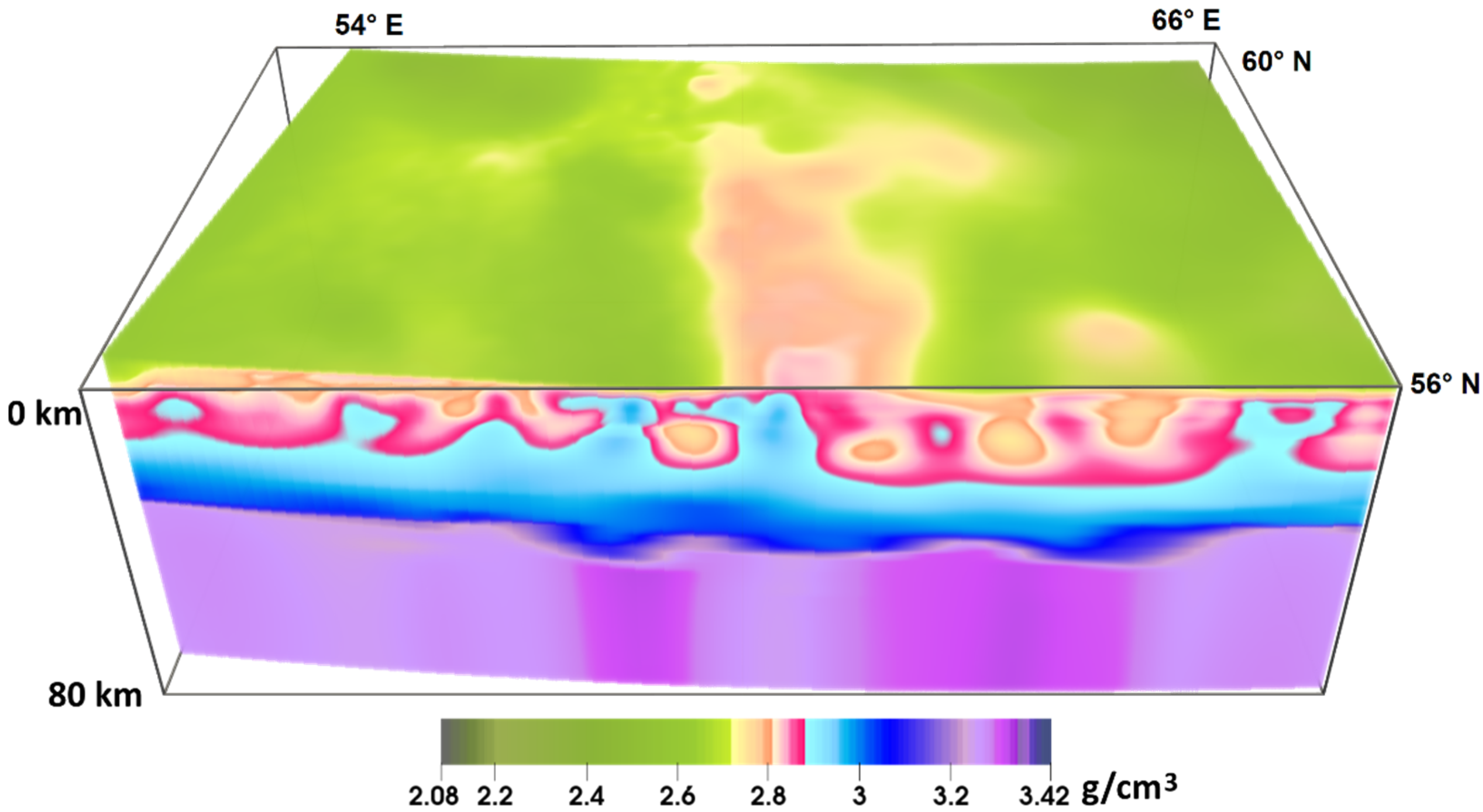
The initial density model frame is formed with the 2D density cuts along the regional profiles (Figure 2). The data between profiles are interpolated values (layer by layer) [3]. The mean value of density (Figure 3) is calculated for each depth of the initial model (Figure 4). This 1D density distribution is continued outside the study volume and the excess density is calculated relative to it. As we seek 3D density distribution as a product of this function, and some 2-dimensional corrective addition , the inverse problem for lateral density in a flat layer will be sufficiently stable [23,26].
The described interpretation algorithm of the gravity data was applied to the difference of the observed field and the initial model field (Figure 5).
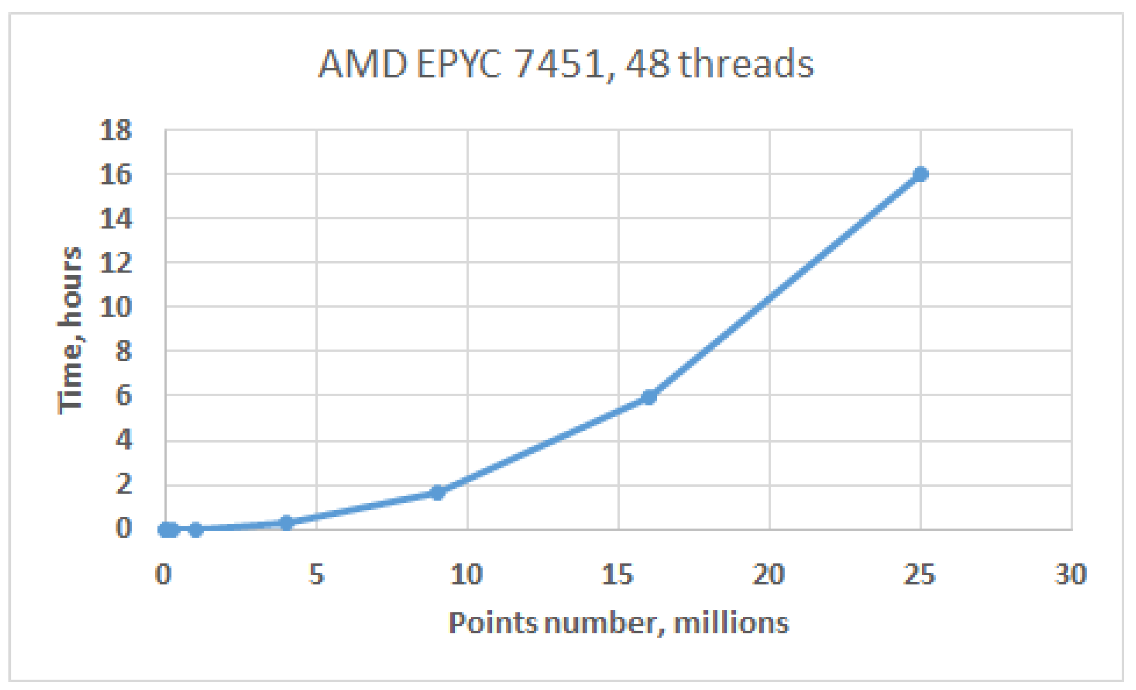
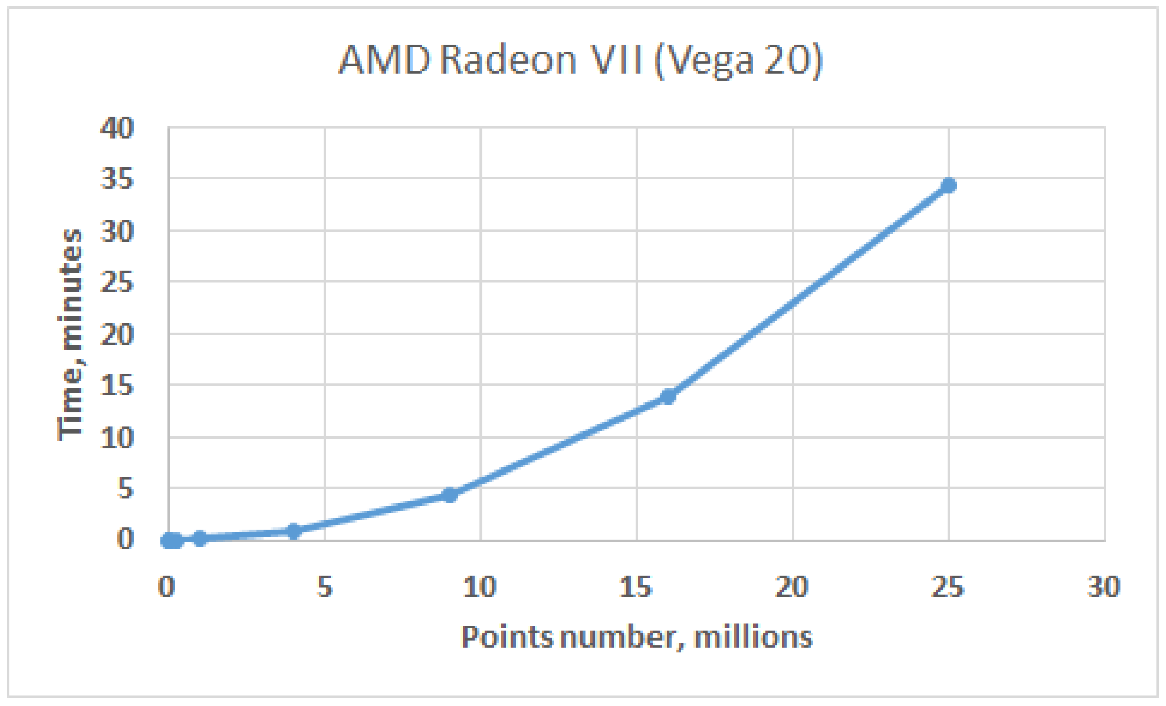
In order to evaluate the acceleration of calculations using the graphics accelerator (GPU) in comparison with the central processing unit (CPU), a series of field upward recalculations was carried out with different sampling grid resolutions. It should be noted that in the calculations, the discretization parameters of the grids of the recalculated and resulting fields were the same. Discretization parameters and computation times are shown in Table 1. The calculations were carried out with 24 cores (48 threads) of the AMD EPYC 7451 processor with a clock frequency of 2.9 GHz and one GPU AMD Radeon VII (Vega 20). Figure 6 and Figure 7 show the corresponding graphs of performance.
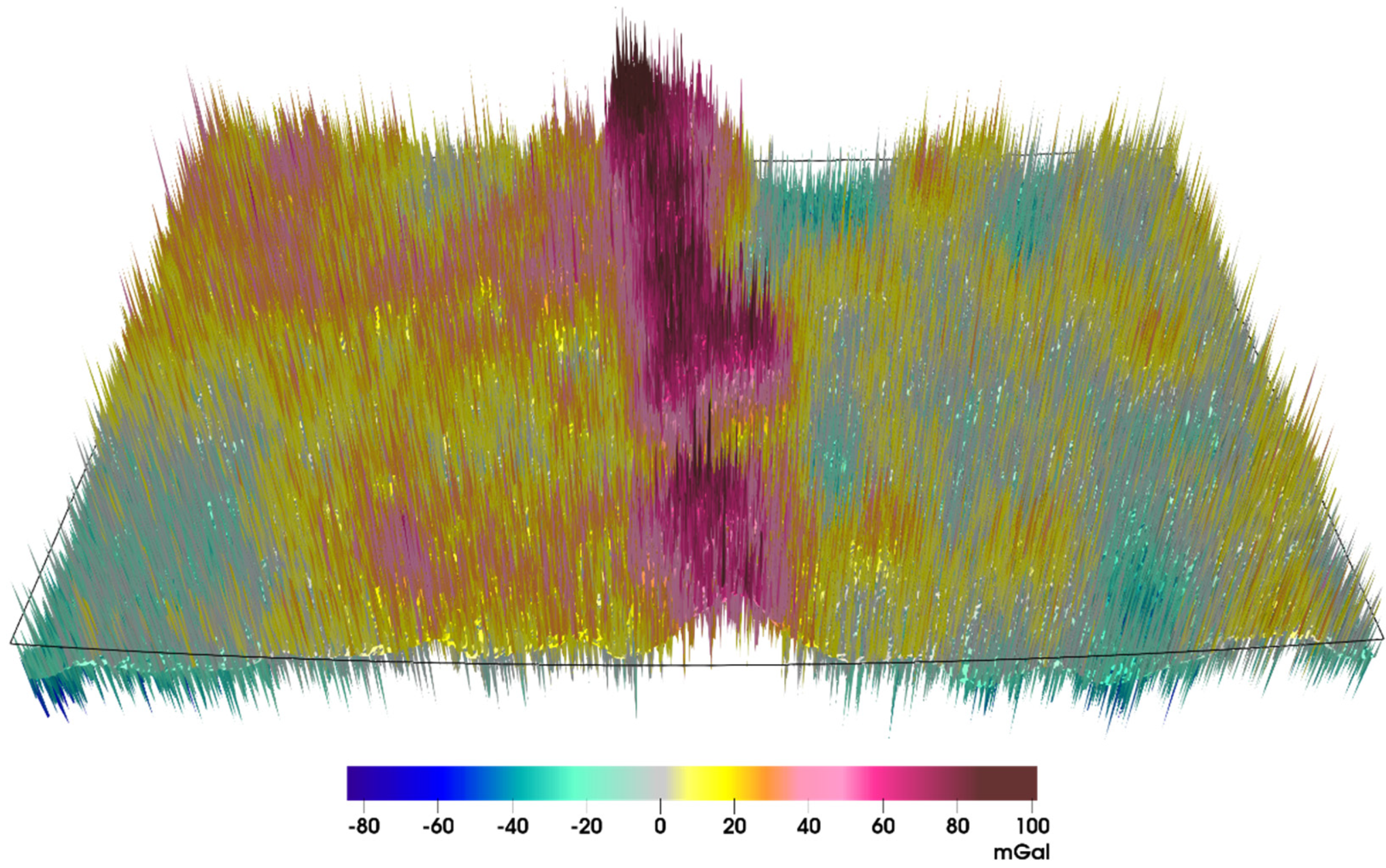
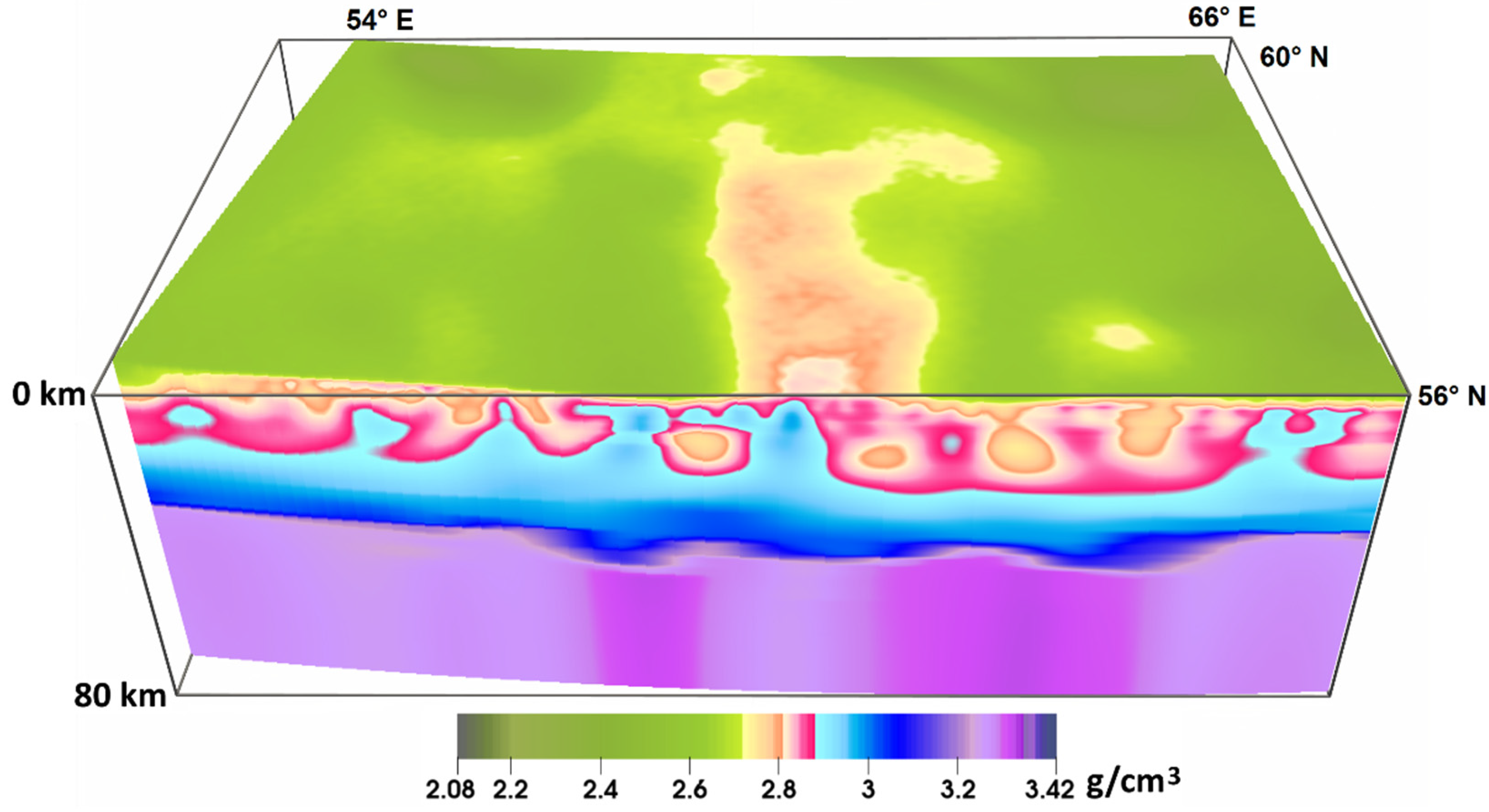
A density model that satisfies the observed data was constructed using the described method. The initial distribution (Figure 3) was used as the input data. Resulting density model (Figure 10) consists of prismatic elements; resolution of this model is 1236 × 1314 × 80. Figure 11 shows the change in the intervals of densities between the initial and the fitted model.
The stability of the proposed method is demonstrated here. To the observed field (Figure 5-(1)), at a random 33% of all points, we add Gaussian noise with zero mean and standard deviation of 6.72 mGal (33% of the standard deviation of the field). Figure 12 shows the result.
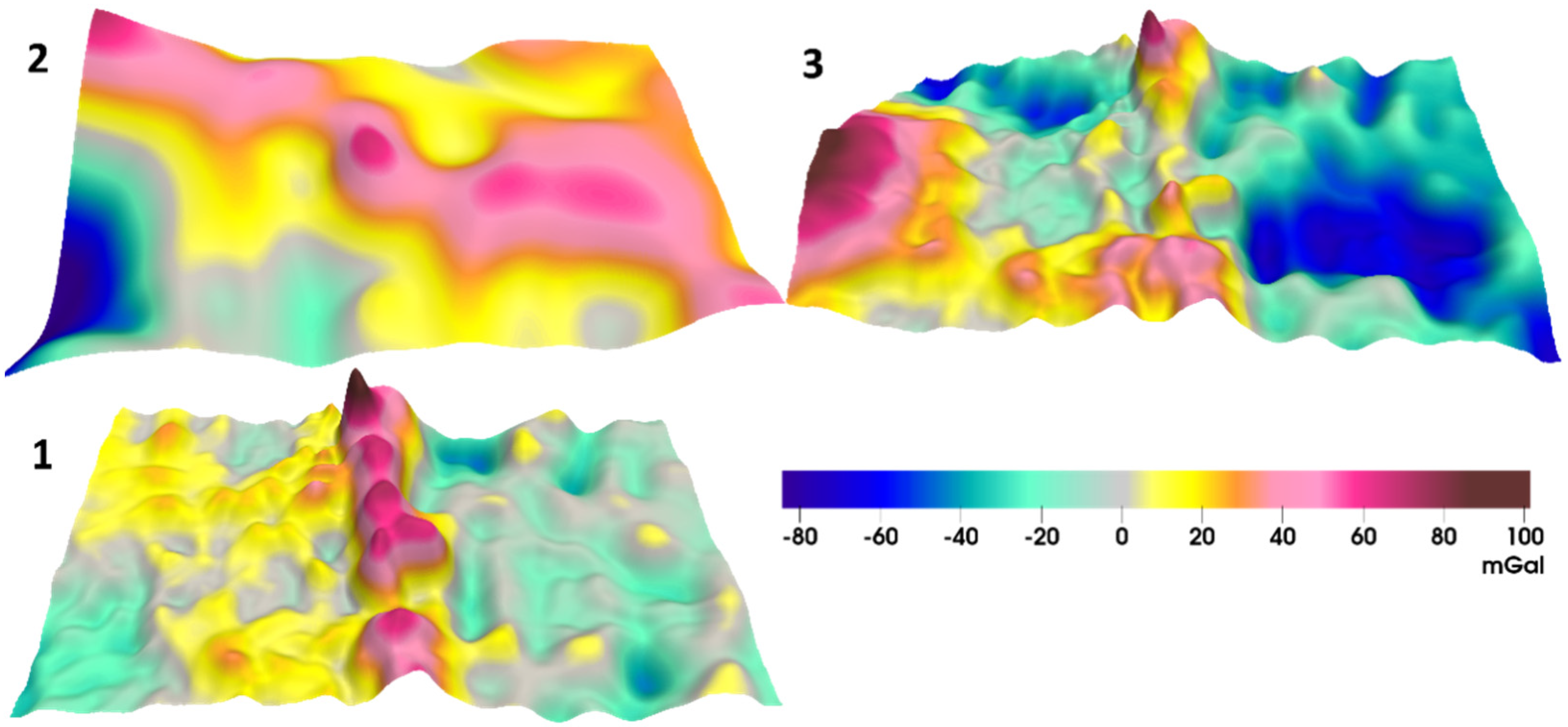
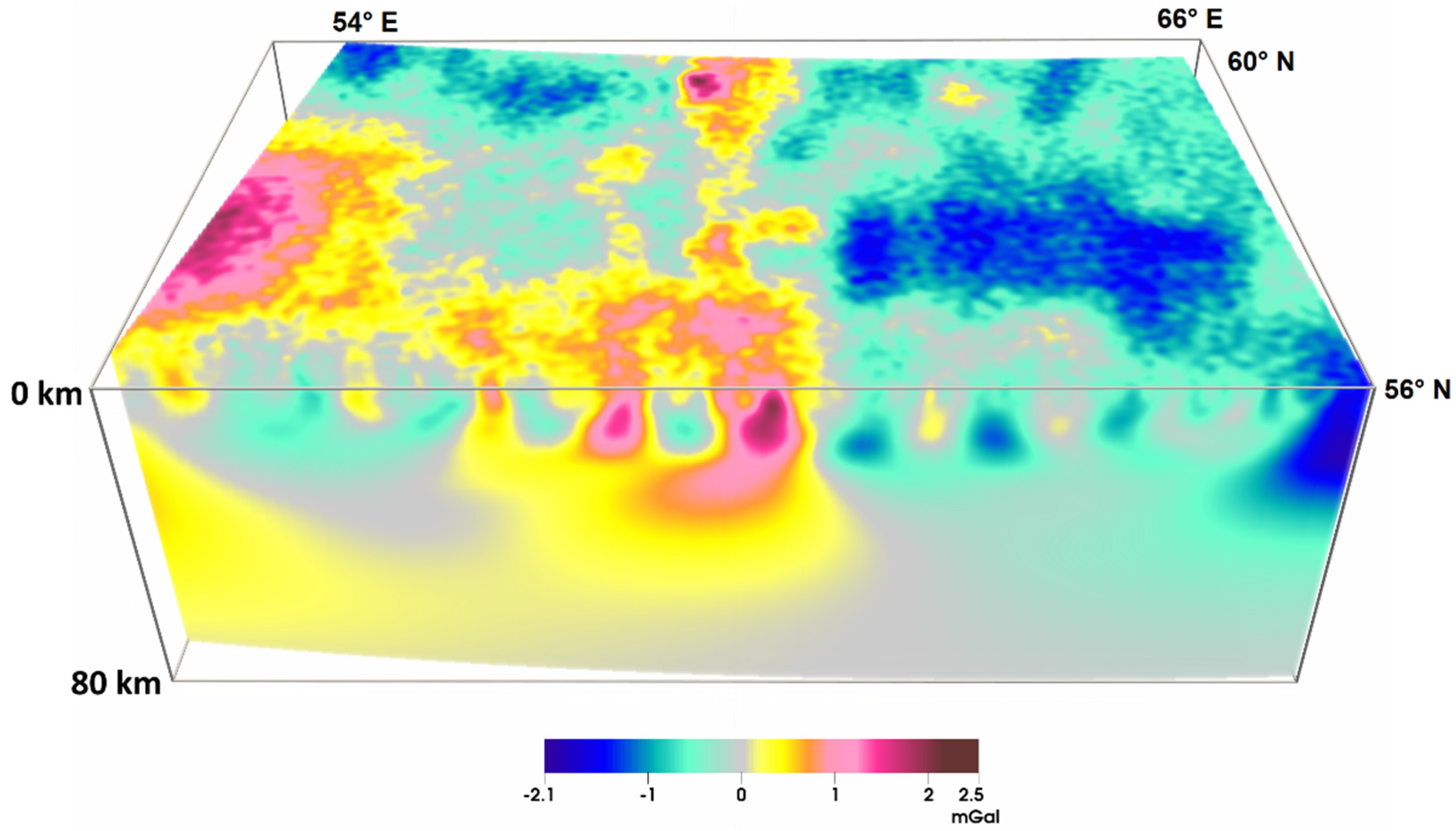
We calculate the difference between the noised field and the initial model field, shown in Figure 5-(2) Then, we apply the above-described recalculation filter to this difference for the layer-by-layer separation of the field up to 80 km in depth with a step of 1 km. Leaving the set of smoothing parameters the same as in the example without noise, the separation result for four thick layers is shown in Figure 13. “Cuboid of the separated fields” for 1 km thick layers is shown in Figure 14.
As can be seen, most of the noise has been filtered out. This is not surprising, because the basis of our filter is Lavrentiev’s regularization. The remnants of the noise “penetrated” to a depth of about 7 km. It should be noted that if we chose a set of smoothing parameters specifically for this case, then the noise could be completely neutralized. This, of course, would also be facilitated by the fact that our original observed field does not have a “high-frequency” component. From a practical point of view, the “noisy” (Figure 15) and “clean” (Figure 10) models coincide.
4. Conclusions
In this study, we offered a method of gravity field interpretation, which uses complete a priori information. The algorithm’s stability is ensured by the selection of the initial model and solving of the problem on the correctness set. The new algorithm is suggested as a preliminary pre-processing of gravity observations that allows the extraction of the gravitational effect of the layers. The modified method of local corrections is developed for the downward continuation of the gravity field. A new method for reconstruction of density distribution using gravity data is presented. Both algorithms are applied to the real gravity data for the Ural region, Russia.
The density model of the initial approximation and the fast original algorithms for solving the gravity problem with high resolution (using parallel computations) allows for the calculation of large-scale density models. Based on the results of the numerical modeling, it is possible to construct a volumetric (gradient) model of the layer-by-layer density distribution in the inhomogeneous layer and, within the framework of the obtained solution, restore the zones of the local inhomogeneity. We have created such 3D model for the study area. Volumetric density models are of considerable practical importance and can be used to justify the location of the prospecting and exploration work in the vicinity of promising areas.
Author Contributions
Conceptualization, P.M. and D.B.; methodology, P.M., I.L. and D.B.; software, D.B.; validation, P.M. and D.B.; formal analysis, P.M.; investigation, P.M., I.L. and D.B.; writing—original draft preparation, P.M. and D.B.; writing—review and editing, P.M., I.L. and D.B.; visualization, D.B.; supervision, P.M.; project administration, P.M.; funding acquisition, P.M. All authors have read and agreed to the published version of the manuscript.
Funding
This research was funded by Russian Science Foundation, grant number 20-17-00058.
Institutional Review Board Statement
Not applicable.
Informed Consent Statement
Not applicable.
Data Availability Statement
Not applicable.
Conflicts of Interest
The authors declare no conflict of interest. The funders had no role in the design of the study; in the collection, analyses, or interpretation of data; in the writing of the manuscript, or in the decision to publish the results.
References
- Cordell, L.; Henderson, R.G. Iterative three-dimensional solution of gravity anomaly data using a digital computer. Geophysics 1968, 33, 596–601. [Google Scholar] [CrossRef]
- Sampietro, D.; Sanso, F. Uniqueness theorems for inverse gravimetric problems. In VII Hotine-Marussi Symposium on Mathematical Geodesy; Springer: Berlin/Heidelberg, Germany, 2012; pp. 111–115. [Google Scholar]
- Martyshko, P.S.; Ladovskiy, I.V.; Tsidaev, A.G. Construction of regional geophysical models based on the joint interpretation of gravitaty and seismic data. Izv. Phys. Solid Earth 2010, 46, 931–942. [Google Scholar] [CrossRef]
- Pašteka, R.; Karcol, R.; Kušnirák, D.; Mojzeš, A. REGCONT: A Matlab based program for stable downward continuation of geophysical potential fields using Tikhonov regularization. Comput. Geosci. 2012, 49, 278–289. [Google Scholar]
- Guoqing, M.; Cai, L.; Danian, H.; Lili, L. A stable iterative downward continuation of potential field data. J. Appl. Geophys. 2013, 98, 205–211. [Google Scholar]
- Tran, K.V.; Nguyen, T.N. A novel method for computing the vertical gradients of the potential field: Application to downward continuation. Geophys. J. Int. 2020, 220, 1316–1329. [Google Scholar] [CrossRef]
- Pitoňák, M.; Novák, P.; Eshagh, M.; Tenzer, R.; Šprlák, M. Downward continuation of gravitational field quantities to an irregular surface by spectral weighting. J. Geod. 2020, 94, 62. [Google Scholar] [CrossRef]
- Abdelazeem, M.; Gobashy, M. A solution to unexploded ordnance detection problem from its magnetic anomaly using Kaczmarz regularization. Interpretation 2016, 4, SH61–SH69. [Google Scholar] [CrossRef]
- Nagy, D. Gravitational attraction of a right rectangular prism. Geophysics 1966, 31, 362–371. [Google Scholar] [CrossRef]
- Baneergee, B.; Gupta, S.P.D. Gravitational attraction of a rectangular parallelepiped. Geophysics 1977, 42, 1053–1055. [Google Scholar] [CrossRef]
- Mostafa, M.E. Finite cube elements method for calculating gravity anomaly and structural index of solid and fractal bodies with defined boundaries. Geophys. J. Int. 2008, 172, 887–902. [Google Scholar] [CrossRef] [Green Version]
- Couder-Castañeda, C.; Ortiz-Alemán, J.C.; Orozco-del-Castillo, M.G.; Nava-Flores, M. Forward modeling of gravitational fields on hybrid multi-threaded cluster. Geofísica Int. 2015, 54, 31–48. [Google Scholar] [CrossRef] [Green Version]
- Dubey, C.P.; Tiwari, V.M. Computation of the gravity field and its gradient: Some applications. Comput. Geosci. 2016, 88, 83–96. [Google Scholar] [CrossRef]
- Li, Y.; Oldenburg, D.W. 3-D inversion of gravity data. Geophysics 1998, 63, 109–119. [Google Scholar] [CrossRef]
- Cai, Y.; Wang, C. Fast finite element calculation of gravity anomaly in complex geological regions. Geophys. J. Int. 2005, 162, 696–708. [Google Scholar] [CrossRef] [Green Version]
- Martyshko, P.S.; Prutkin, I.L. Technology of depth distribution of gravity field sources. Geofiz. Zhurnal (Geophys. J.) 2003, 25, 159–165. (In Russian) [Google Scholar]
- Prutkin, I.; Vajda, P.; Tenzer, R.; Bielik, M. 3D inversion of gravity data by separation of sources and the method of local corrections: Kolarovo gravity high case study. J. Appl. Geophys. 2011, 75, 472–478. [Google Scholar] [CrossRef]
- Martyshko, P.S.; Fedorova, N.V.; Akimova, E.N.; Gemaidinov, D.V. Studying the structural features of the lithospheric magnetic and gravity fields with the use of parallel algorithms. Izv. Phys. Solid Earth 2014, 50, 508–513. [Google Scholar] [CrossRef]
- Prutkin, I.L. The solution of three-dimensional inverse gravimetric problem in the class of contact surfaces by the method of local corrections. Izv. Phys. Solid Earth 1986, 22, 49–55. [Google Scholar]
- Martyshko, P.S.; Ladovskii, I.V.; Byzov, D.D.; Tsidaev, A.G. Gravity data inversion with method of local corrections for finite elements models. Geosciences 2018, 8, 373. [Google Scholar] [CrossRef] [Green Version]
- Blakely, R.J. Potential Theory in Gravity and Magnetic Applications; Cambridge University Press: Cambridge, UK, 1995. [Google Scholar]
- Lavrentiev, M.M. Some Improperly Posed Problems of Mathematical Physics; Springer: Heidelberg, Germany, 1967. [Google Scholar]
- Novoselitskii, V.M. On the theory of determining density variations in a horizontal layer from gravity anomaly data. Izv. Akad. Nauk SSSR Fiz. Zemli 1965, 5, 25–32. [Google Scholar]
- Ince, E.S.; Barthelmes, F.; Reißland, S.; Elger, K.; Förste, C.; Flechtner, F.; Schuh, H. ICGEM—15 years of successful collection and distribution of global gravitational models, associated services and future plans. Earth Syst. Sci. Data 2019, 11, 647–674. [Google Scholar] [CrossRef] [Green Version]
- Ladovskii, I.V.; Martyshko, P.S.; Byzov, D.D.; Kolmogorova, V.V. On selecting the excess density in gravity modeling of inhomogeneous media. Phys. Solid Earth 2017, 53, 130–139. [Google Scholar] [CrossRef]
- Martyshko, P.S.; Ladovskii, I.V.; Byzov, D.D. Solution of the gravimetric inverse problem using multidimensional grids. Dokl. Earth Sci. 2013, 450, 666–671. [Google Scholar] [CrossRef]
Figure 1.
DSS profiles scheme with a map of a gravity field anomaly (XGM2019e_2159) in the Bouguer reduction. (1) Granit + Rubin-2; (2) Krasnouralskiy + Khanty-Mansiyskiy; (3) VNTO; (4) N. Sosva–Yalutorovsk; and (5) Rubin-1; (6) Sverdlovskiy.
Figure 1.
DSS profiles scheme with a map of a gravity field anomaly (XGM2019e_2159) in the Bouguer reduction. (1) Granit + Rubin-2; (2) Krasnouralskiy + Khanty-Mansiyskiy; (3) VNTO; (4) N. Sosva–Yalutorovsk; and (5) Rubin-1; (6) Sverdlovskiy.

Figure 2.
Spatial position of the density profiles constructed with seismic data in the study area. (1) Granit + Rubin-2; (2) Krasnouralskiy + Khanty-Mansiyskiy; (3) VNTO; (4) N. Sosva–Yalutorovsk; (5) Rubin-1; and (6) Sverdlovskiy.
Figure 2.
Spatial position of the density profiles constructed with seismic data in the study area. (1) Granit + Rubin-2; (2) Krasnouralskiy + Khanty-Mansiyskiy; (3) VNTO; (4) N. Sosva–Yalutorovsk; (5) Rubin-1; and (6) Sverdlovskiy.

Figure 3.
Initial dependency of average density value versus depth (black line). Minimum (blue line) and maximum (red line) density values on corresponding depth levels are also shown.
Figure 3.
Initial dependency of average density value versus depth (black line). Minimum (blue line) and maximum (red line) density values on corresponding depth levels are also shown.

Figure 4.
Initial 3D density model (model with the interpolated density).

Figure 5.
Gravity field: (1) observed; (2) initial model; and (3) difference.

Figure 6.
Dependence of computation time with the CPU AMD EPYC 7451 (48 threads) on the number of field evaluation points.
Figure 6.
Dependence of computation time with the CPU AMD EPYC 7451 (48 threads) on the number of field evaluation points.

Figure 7.
Dependence of calculation time with the GPU AMD Radeon VII on the number of field evaluation points.
Figure 7.
Dependence of calculation time with the GPU AMD Radeon VII on the number of field evaluation points.

Figure 8.
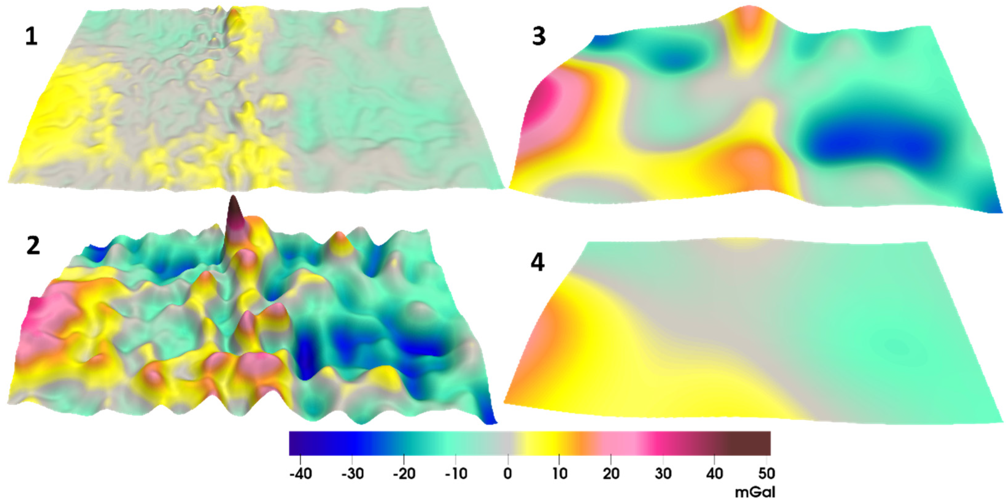
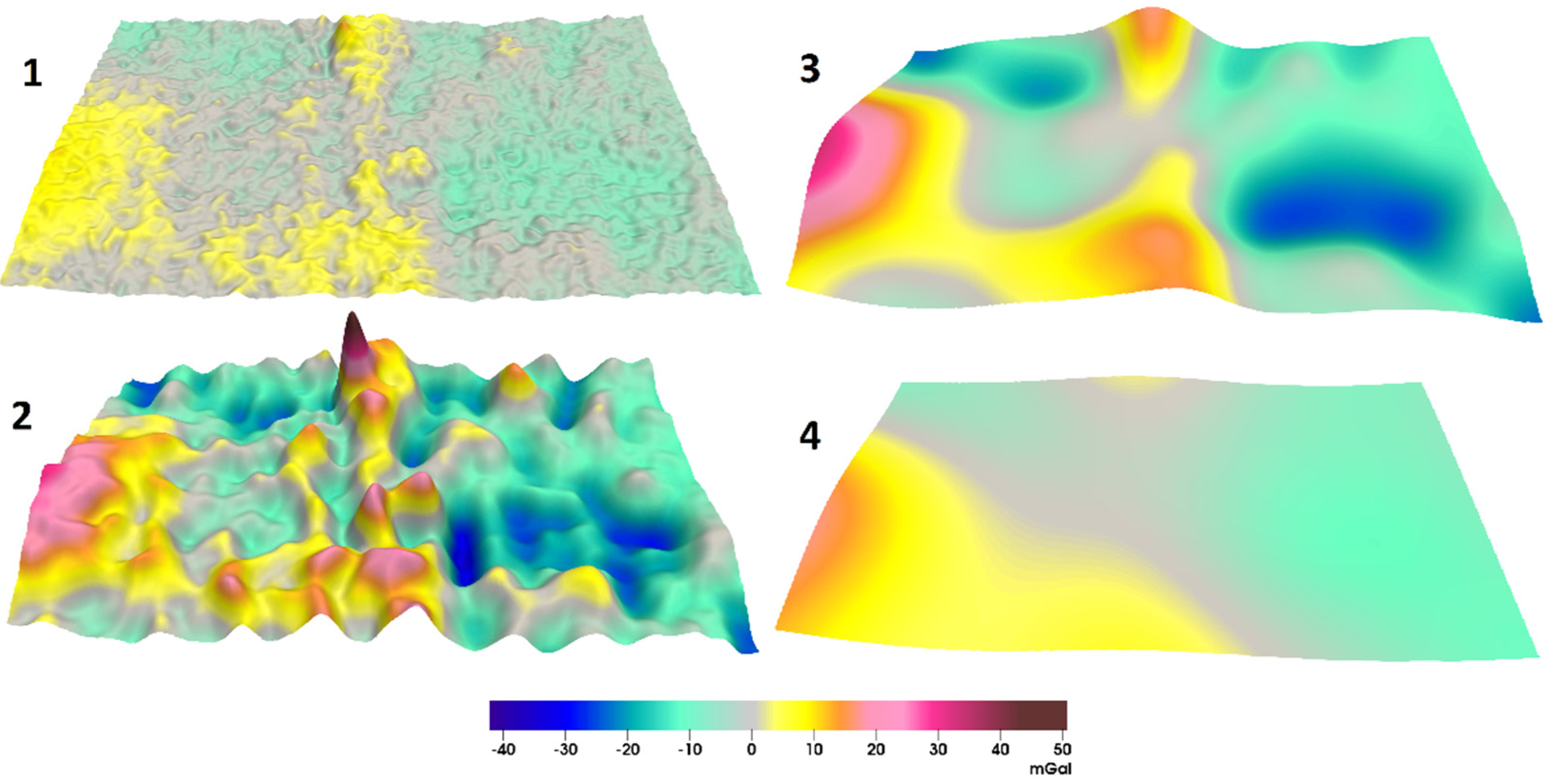
Examples of the different field separations. The minimum and maximum of amplitude of the field are also shown. The ranges of depths of the layer are (1) H ∊ [0, 5] km, Δg ∊ [−8.8, 15.1] mGal; (2) H ∊ [5, 20] km, Δg ∊ [−35.3, 54.3] mGal; (3) H ∊ [20, 40] km, Δg ∊ [−26.7, 34.8] mGal; and (4) H ∊ [40, 80] km, Δg ∊ [−12.2, 17.7] mGal. The masses in the layer are considered to be the sources of the separated field.
Figure 8.
Examples of the different field separations. The minimum and maximum of amplitude of the field are also shown. The ranges of depths of the layer are (1) H ∊ [0, 5] km, Δg ∊ [−8.8, 15.1] mGal; (2) H ∊ [5, 20] km, Δg ∊ [−35.3, 54.3] mGal; (3) H ∊ [20, 40] km, Δg ∊ [−26.7, 34.8] mGal; and (4) H ∊ [40, 80] km, Δg ∊ [−12.2, 17.7] mGal. The masses in the layer are considered to be the sources of the separated field.

Figure 9.
“Cuboid of the separated fields”. The Layers are 1 km thick.

Figure 10.
Fitted 3D density model.

Figure 11.
Graphs of the dependence of the minimum (blue line), maximum (red line) and mean (black line) density of the initial (dash line) and fitted (solid line) models on the depth.
Figure 11.
Graphs of the dependence of the minimum (blue line), maximum (red line) and mean (black line) density of the initial (dash line) and fitted (solid line) models on the depth.

Figure 12.
Noised observed field.

Figure 13.
Examples of the noised different field separation. The ranges of depths of the layer are (1) H ∊ [0, 5] km, Δg ∊ [−9.7, 13.8] mGal; (2) H ∊ [5, 20] km, Δg ∊ [−33.0, 50.2] mGal; (3) H ∊ [20, 40] km, Δg ∊ [−25.6, 33.5] mGal; and (4) H ∊ [40, 80] km, Δg ∊ [−11.8, 17.1] mGal.
Figure 13.
Examples of the noised different field separation. The ranges of depths of the layer are (1) H ∊ [0, 5] km, Δg ∊ [−9.7, 13.8] mGal; (2) H ∊ [5, 20] km, Δg ∊ [−33.0, 50.2] mGal; (3) H ∊ [20, 40] km, Δg ∊ [−25.6, 33.5] mGal; and (4) H ∊ [40, 80] km, Δg ∊ [−11.8, 17.1] mGal.

Figure 14.
“Cuboid of the separated fields”. The layers are 1 km thick.

Figure 15.
Fitted 3D density model for noised field.


Table 1.
Dependence of the computation time on the discretization parameters of the field evaluation grid.
Table 1.
Dependence of the computation time on the discretization parameters of the field evaluation grid.
| Nx × Ny | N = Nx × Ny, 106 Points | CPU Calculation Time, min | GPU Calculation Time, min |
|---|---|---|---|
| 200 × 200 | 0.04 | 7.3 × 10⁻⁴ | 5 × 10⁻⁵ |
| 500 × 500 | 0.25 | 0.072 | 4.9 × 10⁻³ |
| 1000 × 1000 | 1 | 0.95 | 0.065 |
| 2000 × 2000 | 4 | 16.5 | 0.86 |
| 3000 × 3000 | 9 | 99.6 | 4.4 |
| 4000 × 4000 | 16 | 354.6 | 13.9 |
| 5000 × 5000 | 25 | 958.7 | 34.5 |
Publisher’s Note: MDPI stays neutral with regard to jurisdictional claims in published maps and institutional affiliations. |
© 2021 by the authors. Licensee MDPI, Basel, Switzerland. This article is an open access article distributed under the terms and conditions of the Creative Commons Attribution (CC BY) license (https://creativecommons.org/licenses/by/4.0/).
Share and Cite
MDPI and ACS Style
Martyshko, P.; Ladovskii, I.; Byzov, D. Parallel Algorithms for Solving Inverse Gravimetry Problems: Application for Earth’s Crust Density Models Creation. Mathematics 2021, 9, 2966. https://0-doi-org.brum.beds.ac.uk/10.3390/math9222966
AMA Style
Martyshko P, Ladovskii I, Byzov D. Parallel Algorithms for Solving Inverse Gravimetry Problems: Application for Earth’s Crust Density Models Creation. Mathematics. 2021; 9(22):2966. https://0-doi-org.brum.beds.ac.uk/10.3390/math9222966
Chicago/Turabian StyleMartyshko, Petr, Igor Ladovskii, and Denis Byzov. 2021. "Parallel Algorithms for Solving Inverse Gravimetry Problems: Application for Earth’s Crust Density Models Creation" Mathematics 9, no. 22: 2966. https://0-doi-org.brum.beds.ac.uk/10.3390/math9222966
Note that from the first issue of 2016, this journal uses article numbers instead of page numbers. See further details here.