Graph, Spectra, Control and Epidemics: An Example with a SEIR Model

Abstract

Networks and graphs offer a suitable and powerful framework for studying the spread of infection in human and animal populations. In the case of a heterogeneous population, the social contact network has a pivotal role in the analysis of directly transmitted infectious diseases. The literature presents several works where network-based models encompass realistic features (such as contacts networks or host–pathogen biological data), but analytical results are nonetheless scarce. As a significant example, in this paper, we develop a multi-group version of the epidemiological SEIR population-based model. Each group can represent a social subpopulation with the same habits or a group of geographically localized people. We consider also heterogeneity in the weighting of contacts between two groups. As a simple application, we propose a simple control algorithm in which we optimize the connection weights in order to minimize the combination between an economic cost and a social cost. Some numerical simulations are also provided.

1. Introduction

The epidemiological modeling of infectious disease transmission has a long history in mathematical biology, for humans [1,2,3,4,5,6,7], animals [3,8] and plants [9,10,11]. In recent years it has had an increasing influence on the theory and practice of disease management and control, e.g., [12,13,14,15,16,17,18]. Indeed the forecast of the spread of an infectious disease is critical to public health decision making.

The proper modeling and analysis of the dynamics of infectious diseases has been a long-standing area of research among many different fields, including economics, social sciences, mathematical biology, physics, computer science and engineering [5]. In the classical population approach, the underlying common factor is the partitioning of the population into “compartments”; we assume that the populations in the various compartments are homogenous in the sense that all individuals behave similarly. The two most common compartments that exist in almost all epidemic models are susceptible (S) and infected (I) [2,3]. The subpopulation S represents individuals who are healthy but susceptible to becoming infected, while I represents individuals who became infected but are able to recover. If the model contains only these two compartments, a given population is initially divided into them. From this basic compartmentalization, there are numerous ways for introducing different interactions within the population. Most of these models for the disease evolution make two basic assumptions. The first assumption states that the population is well-mixed. In such a population, each individual has the same probability of encountering other infected individuals, and thus the resulting force of infection is equal for all. The second assumption states that there are a priori constraints upon the biological process, whilst gradual but random mutation of disease traits (such as transmission rate and infectious period) could occur. More refined epidemic models are required; the entire population cannot just be divided into two or more compartments/groups which are defined by a single quantity. In this paper, we consider the effect of the heterogeneity in the weighting of contacts between two individuals. Moreover, we focus on a meta-population model where the population is previously subdivided into subpopulations that can consist in spatially distinct groups of individuals (neighborhoods, towns, cities, etc.) or groups of individuals with different features. The resulting model is described by a dynamic system defined on a network (graph). We have also added the possibility of varying the weight of the connections between groups in order to formalize the problem of controlling the spread of the epidemic on the network. This generality could also allow the changing of disease features.

The paper is organized as follows: Section 2 introduces the model and the analysis of the corresponding dynamical system. Moreover, as an application of this approach, we will also discuss a new definition of control problem about the spread of epidemics on the network. Section 3 is devoted to numerical experiments using a reduced network with different features. Following the findings of the case study and of previous analysis, the conclusions are presented in Section 4.

2. A Meta-Population Model on a Network

The transmission of infectious diseases raises many important questions. In some instances, the average behavior of a large population with respect to the time is sufficient to provide useful insight from the available data. However, the spatial component of many transmission systems has been recognized to be of pivotal importance in the recent years. Due to this, spatially heterogeneous interventions must be included in the model, and hence it is essential to properly represent the transmission pattern. A reasonable hypothesis may consider that the spatial aspects of transmission heavily influence the aggregation characteristic of epidemic influence. Hence, we need to investigate data by using models that include such spatial connections. For example, the understanding of human mobility and the developing of qualitative and quantitative theories is of key importance for the modeling and for the comprehension of human infectious disease dynamics on geographical scales of different size.

2.1. Spatial Heterogeneity in Epidemiological Models

Ideally, the model should be able to account for the states of all N individuals in the population in an independent manner and, at the same time, it should allow for arbitrary interactions among them. The analysis of these models is a difficult task, and the computational cost of numerical simulations is very onerous and the extraction of the collective behaviors very complex. Although studies on the temporal dynamics of diseases proved insightful, incorporating space explicitly into epidemiological models revealed various emergent properties [19]. The phenomenon of the spatial spread of infection involves several components and scale [20]. Indeed, small region/group models can incorporate spatial heterogeneity, and more general models allowing for larger households with continuous or discrete time can be developed. Other typical approaches encompassing spatial variation in epidemic models involve partial differential equations (PDE). There exist, nonetheless, cases and scenarios where the latter type of spatial approach may not reliably model the phenomenon. Consider, for example, a human specific disease which is spread only by person-to-person contact and consider a geographical context consisting in a large country with a small number of large cities and a very sparse (or even non-existent) rural population [21]. The travel of individuals between discrete geographical regions and/or cities plays a pivotal role in the disease spreading. The depicted situation is easily described by a directed graph, where the vertices represent the cities (or discrete geographical regions/patches) and the arcs represent the links between such cities [22].

The main approaches for spatial models concern a different scale: an individual-based simulation, a meta-population model or a network model (see, e.g., [14]). Individual-based models explicitly represent every individual i with a state $X_i\left(t\right)$ at time t, e.g., $X_i\left(t\right)=1$ indicates that i is infected while $X_i\left(t\right)=0$ indicates that i is healthy at time t. Infected nodes can transmit the disease to neighboring nodes and an individual becomes infected with a certain probability based on the status of neighboring individuals. The meta-population framework consists of dividing the whole population into distinct subpopulations, each having independent internal dynamics. In addition, at the same time, there is a limited interaction between the subpopulations. This approach has been used to great effect within ecological systems [23,24]. The individuals in such subpopulations belong to a particular state (e.g., susceptible or infectious) which can change during the time. For large networks, a general approach consists of merging some network information in a relatively small set of statistics and then studying the impact of such statistics on the infection spread [25].

In the following section, we describe our meta-population model, which considers communities as the aggregate unit that may represent either subpopulations in different areas or distinct groups with similar characteristics (e.g., students on a campus and citizens of a neighborhood or high school students or office workers). Then, each subpopulation is partitioned according to a particular state of individuals with respect to disease. Finally, connections and mobility between different communities are introduced. We point out that various proposed models encompass the geography of spread of the disease, but they do not present a mathematical analysis of their main properties, while presenting realistic simulations and an appropriate identification of the parameters involved, e.g., [26].

2.2. A Prototype: SEIR Model on a Direct Graph

We introduce a prototype model that can be generalized considering several states related to a given disease. Our analysis can, therefore, easily be extended to these more complex models. We partition a population of N individuals into subpopulations (groups, patches, communities, etc.) without taking into account any biological interpretation they have but considering spatially segregated large subpopulations. In this way, we can encompass a more realistic contact structure into epidemic models, since it usually preserves analytic tractability (in stochastic and in deterministic models), but at the same time it also captures the most important structural inhomogeneity in contact patterns in several applied contexts. The subpopulations and the interactions/connections between them are modeled through a weighted direct graph $\mathcal{G}=(\mathcal{V},\mathcal{E})$ with n vertices (nodes, regions, patches, subpopulations) and m edges (connections). Each edge is described by an ordered pairs of nodes $(u,v)$, where $u,v\in \mathcal{V}$. We label the nodes with an integer index; two vertices i and j of the directed graph are joined or adjacent if and only if there exists an edge from i to j or from j to i. If such an edge exists, then i and j are called its endpoints. If there is an edge from i to j then i and j are often called tail and head, respectively. The $(n\times n)$ adjacency matrix $A^d$ associated to the graph is constructed as follows: if there exists an edge from node i to node j, then the entry at row i and column j is set to 1 in the matrix $A^d$: $a_{ij}^d=1$.

In node i, the corresponding subpopulation possesses $N_i$ individuals, and ${\sum }_{i=1}^n{N}_i=N$. We hypothesize that individuals can move to a different node, interact with people in that node and then return to the original one. If $a_{ij}^d=1$, there is an interaction between node i and node j, but not all the subpopulation $N_i$ from node i interacts with the population in node j: we denote by $a_{ij}$ the total amount of the subpopulation i that “goes” to node j and interacts with the people in that node. We call A the routing matrix with entries $a_{ij}$, so that ${\sum }_{j=1}^n{a}_{ij}=N_i$, $i=1,\cdots ,n$. Associated to A, let $P^o$ the probability outgoing matrix with entries $p_{ij}^o$, where we denote by $p_{ij}^o$ the percentage (probability) of the subpopulation i that “goes” to node j. In addition, we denote by $P^i$ the probability incoming matrix with entries $p_{ij}^i$, where $p_{ij}^i$ is now the percentage (probability) of the subpopulation in j that “arrived” from i. Finally, let $M_i={\sum }_{j=1}^n{a}_{ji}$ be the total amount of people arrived in node $i=1,\cdots ,n$, so that ${\sum }_{i=1}^n{M}_i=N$ again. Then, for any $i=1,\cdots ,n$, ${\sum }_{j=1}^n{p}_{ij}^o={\sum }_{j=1}^n{p}_{ji}^i=1$. Moreover we have

$$A=Diag(N_1,N_2,\cdots ,N_n)P^o=P^{i}Diag(M_1,M_2,\cdots ,M_n)$$

where $Diag(x_1,x_2,\cdots ,x_n)$ is the diagonal matrix with the vector ${(x_1,x_2,\cdots ,x_n)}^T\in {\mathbb{R}}^n$ on the main diagonal.

Four different discrete classes are considered for statuses of individuals in each: susceptible, exposed, infectious and recovered (SEIR model) [2]. All individuals are born as susceptible: a susceptible individual in contact with an infectious one may become exposed; the probability depends on the particular strain of the disease. Exposed individuals are infected but not yet infectious: individuals experience a long incubation duration. With a suitable incubation rate, latent individuals become infectious. Finally, a reliable assumption is that the immune system of infectious individuals combats the infection and then they move directly into the recovered class, which refers to individuals that are no longer infectious and have gained full immunity from further infection. Let $S\left(t\right),E\left(t\right),I\left(t\right),R\left(t\right)$ the number of individuals in a node at time t, $S\left(t\right)+E\left(t\right)+I\left(t\right)+R\left(t\right)=N$: we consider a time interval in which we can neglect demographics. Without any interaction with other nodes, within a deterministic approach of the compartmental models, with continuous time t, the epidemic dynamics can be described by the system of differential equations in (1):

$$\begin{array}{c}\dot{S}\left(t\right)=-\lambda S\left(t\right)\hfill \\ \dot{E}\left(t\right)=\lambda S\left(t\right)-\mu E\left(t\right)\hfill \\ \dot{I}\left(t\right)=\mu E\left(t\right)-\gamma I\left(t\right)\hfill \\ \dot{R}\left(t\right)=\gamma I\left(t\right)\hfill \end{array}$$

(1)

where the parameter $\lambda$ is the force of infection, $\gamma$ is the recovery rate and $1/\mu$ is an average latent period.

With respect to the behavior of an epidemic, $\lambda$ is the rate at which susceptible individuals become infected or exposed and it is a function depending on the number of infectious individuals; it contains information about the interactions between individuals that concur to the infection transmission. If we suppose that the population of N individuals mixes at random, meaning that all pairs of individuals have the same probability of interacting, the force of infection may be computed as:

$$\begin{array}{cc}\lambda \hfill & =\mathrm{transmission}\mathrm{rate}\hfill \\ & \times \mathrm{effective}\mathrm{number}\mathrm{of}\mathrm{contacts}\mathrm{per}\mathrm{unit}\mathrm{time}\hfill \\ & \times \mathrm{proportion}\mathrm{of}\mathrm{contacts}\mathrm{infectious}\hfill \\ & \sim \tau \times n_c\times \frac{I}{N}=\beta \frac{I}{N}\hfill \end{array}$$

Then the dynamics state,

$$\begin{array}{c}\dot{S}\left(t\right)=-\beta \frac{I}{N}S\left(t\right)\hfill \\ \dot{E}\left(t\right)=\beta \frac{I}{N}S\left(t\right)-\mu E\left(t\right)\hfill \end{array}$$

(2)

where $\beta$ is the infectious rate. Rescaling the quantities $S,E,I,R$ dividing by N we obtain,

$$\begin{array}{c}\dot{s}\left(t\right)=-\beta \mathit{ı}\left(t\right)s\left(t\right)\hfill \\ \dot{e}\left(t\right)=\beta \mathit{ı}\left(t\right)s\left(t\right)-\mu e\left(t\right)\hfill \\ \dot{\mathit{ı}}\left(t\right)=\mu e\left(t\right)-\gamma \mathit{ı}\left(t\right)\hfill \\ \dot{r}\left(t\right)=\gamma \mathit{ı}\left(t\right)\hfill \end{array}$$

(3)

Pay attention to the fact that $\dot{\mathit{ı}}$ stands for the derivative of the function ı. Now, we take a node j that is connected to the other nodes as encoded in matrix A. Then, $S_j\left(t\right)$ can change due to the contribution of susceptible people from j that reached an adjacent node k and met infectious people in that node, wheresoever they came from. Then the contribution to ${\dot{S}}_j$ due to the interactions in node k is given by the $p_{jk}^o{S}_j=a_{jk}{s}_j$ susceptible people that met a population in node k with a proportion of infectious people given by

$$\begin{array}{cc}\hfill \frac{\#\left\{\mathrm{infectious}\mathrm{people}\mathrm{in}\mathrm{node}k\right\}}{\#\left\{\mathrm{total}\mathrm{people}\mathrm{in}\mathrm{node}k\right\}}& =\frac{{\sum }_{l=1}^n{p}_{lk}^o{I}_l}{{\sum }_{l=1}^n{a}_{lk}}=\frac{{\sum }_{l=1}^n{p}_{lk}^o{I}_l}{M_k}\hfill \\ & =\frac{{\sum }_{l=1}^n{a}_{lk}{\mathit{ı}}_l}{{\sum }_{l=1}^n{a}_{lk}}=\sum _{l=1}^n{p}_{lk}^i{\mathit{ı}}_l.\hfill \end{array}$$

Let the vectors $\mathbf{X}\left(t\right)={(x_1\left(t\right),x_2\left(t\right),\cdots ,x_n\left(t\right))}^T\in {\mathbb{R}}^n$, with $X=S,E,I,R$, the $SEIR$ model on the graph $\mathcal{G}$ is the following

$$\begin{array}{cccc}\hfill & \dot{\mathit{S}}\left(t\right)=-\beta Diag\left(\mathit{S}\left(t\right)\right)\widehat{B}\mathit{I}\left(t\right)\hfill & \hfill & \dot{\mathit{s}}\left(t\right)=-\beta Diag\left(\mathit{s}\left(t\right)\right)B\mathit{ı}\left(t\right)\hfill \\ \hfill & \dot{\mathit{E}}\left(t\right)=\beta Diag\left(\mathit{S}\left(t\right)\right)\widehat{B}\mathit{I}\left(t\right)-\mu \mathit{E}\left(t\right)\hfill & \hfill & \dot{\mathit{e}}\left(t\right)=\beta Diag\left(\mathit{s}\left(t\right)\right)B\mathit{ı}\left(t\right)-\mu \mathit{e}\left(t\right)\hfill \\ \hfill & \dot{\mathit{I}}\left(t\right)=\mu \mathit{E}\left(t\right)-\gamma \mathit{I}\left(t\right)\hfill & \hfill & \dot{\mathit{ı}}\left(t\right)=\mu \mathit{e}\left(t\right)-\gamma \mathit{ı}\left(t\right)\hfill \\ \hfill & \dot{\mathit{R}}\left(t\right)=\gamma \mathit{I}\left(t\right)\hfill & \hfill & \dot{\mathit{r}}\left(t\right)=\gamma \mathit{ı}\left(t\right)\hfill \end{array}$$

(4)

where $\widehat{B}=P^{o}Diag{(M_1,\dots ,M_n)}^{-1}{P^o}^{\top }$, $B=P^o{P^i}^{\top }$, and the equations on the right side have been obtained by a premultiplication with $Diag{(N_1,N_2,\dots ,N_n)}^{-1}$.

Remark 1.

We have assumed that the parameter β is the same in all nodes. It is possible to easily introduce a different parameter for each node considering more heterogeneity in the model.

In the following, we adopt the notations $\mathbf{1}={[1,1,\dots ,1]}^{\top }$, $\mathbf{0}={[0,0,\dots ,0]}^{\top }$, for any vectors $x,y\in {\mathbb{R}}^n$, $x\ll y\iff x_i<y_i,i=1,2,\dots ,n$; $x\le y\iff x_i\le y_i,i=1,2,\dots ,n$ (and $x<y$ if $x\le y$ but $x\ne y$).

We suppose that the directed graph $\mathcal{G}$ is strongly connected, i.e., there exists a path in each direction between each pair of vertices of the graph, then the matrices A and P are irreducible. This means that we cannot divide the nodes of the graph into two subsets such that there are no connections between the nodes of the two subsets but only within each subset. It also follows that the matrix B is a non-negative irreducible $n\times n$ matrix; by the Perron–Frobenius theorem [27] we deduce:

• B has a positive real eigenvalue equal to its spectral radius $\rho \left(B\right)$;
• There exists an eigenvector $\mathit{v}\gg 0$ corresponding to $\rho \left(B\right)$;
• $\rho \left(B\right)$ increases when any entry of B increases;
• $\rho \left(B\right)$ is a simple eigenvalue of B;
• Collatz–Wielandt formula: $\rho \left(B\right)={min}_{\mathit{x}>\mathbf{0}}{max}_{i:x_i>0}\frac{{\left[{\mathit{x}}^{\top }B\right]}_i}{x_i}={max}_{\mathit{x}>\mathbf{0}}{min}_{i:x_i>0}\frac{{\left[{\mathit{x}}^{\top }B\right]}_i}{x_i}$ that are reached identically on every component of the eigenvector: $\rho \left(B\right)=\frac{{\left[{\mathit{v}}^{\top }B\right]}_i}{v_i}$, for any $i=1,\dots ,n$;
• There is no other, unless rescaled, non-negative eigenvector of B, different from $v$.

Let $B_{\mathit{s}}\left(t\right)=Diag\left(\mathit{s}\left(t\right)\right)B$, ${\lambda }_{\mathit{s}}\left(t\right)=\rho \left(B_{\mathit{s}}\left(t\right)\right)$ the dominant eigenvalue of $B_{\mathit{s}}\left(t\right)$ and $v_{\mathit{s}}\left(t\right)\gg 0$ the corresponding positive left eigenvector.

It is easy to prove that this system of differential equations has a local solution by standard argument by the Cauchy–Lipschitz–Picard–Lindelöf theorem. Furthermore, if $\mathit{ı}\left(0\right)>0$ and $\mathit{s}\left(0\right)\gg 0$ then

• $\mathit{ı}\left(t\right)>0$, and $\mathit{s}\left(t\right)\gg 0$ for all $t>0$;
• $\forall t_1>t_2>0$, $\mathit{s}\left(t_2\right)\gg \mathit{s}\left(t_1\right)$;
• ${\lambda }_{\mathit{s}}\left(t\right)$ is monotone decreasing.

Then, the solution is non-negative. Moreover, it is easy to check that if $s_j\left(0\right)+e_j\left(0\right)+i_j\left(0\right)+r_j\left(0\right)=1$ then $s_j\left(t\right)+e_j\left(t\right)+i_j\left(t\right)+r_j\left(t\right)=1$ and the solution is bounded, so there is a global solution for any time $t>0$.

About the behavior of the epidemic dynamics, we will analyze the most important epidemiological properties:

• The threshold phenomenon that states that, under some condition, an epidemic propagates, in the sense that the introduction of a percentage of infected in the population triggers the contamination of many other individuals, otherwise the epidemic fades off.
• The asymptotic profiles of the steady states in order to understand if an endemic level can be reach.

Theorem 1

(Asymptotic behavior). Denote by ${\mathit{x}}_{\mathit{s}}\left(t\right)$ the normalized version of ${\mathit{v}}_{\mathit{s}}\left(t\right)$: ${\mathit{x}}_{\mathit{s}}{\left(t\right)}^{\top }$$B_{\mathit{s}}\left(t\right)={\lambda }_{\mathit{s}}\left(t\right){\mathit{x}}_{\mathit{s}}{\left(t\right)}^{\top }$ and ${\mathit{x}}_{\mathit{s}}{\left(t\right)}^{\top }{\mathit{x}}_{\mathit{s}}\left(t\right)=1$. For any initial condition, ${\lambda }_{\mathit{s}}\left(t\right)$ is a continuous function, and there exist the limits of the above quantities: ${\mathit{s}}_{\infty }={lim}_{t\to \infty }\mathit{s}\left(t\right)$, ${lim}_{t\to \infty }{B}_{\mathit{s}}\left(t\right)=B_{{\mathit{s}}_{\infty }}=Diag\left({\mathit{s}}_{\infty }\right)B$, ${lim}_{t\to \infty }{\lambda }_{\mathit{s}}\left(t\right)={\lambda }_{{\mathit{s}}_{\infty }}$, where $\rho \left(B_{{\mathit{s}}_{\infty }}\right)={\lambda }_{{\mathit{s}}_{\infty }}$.

If ${\mathit{s}}_{\infty }>0$, then $\rho \left(B_{{\mathit{s}}_{\infty }}\right)={\lambda }_{\infty }>0$ and any converging subsequence of ${\mathit{x}}_{\mathit{s}}\left(t\right)$ converges to a ${\lambda }_{\infty }$-eigenvector.

If, in addition, ${\mathit{s}}_{\infty }\gg 0$, ${\lambda }_{\infty }$ is simple, and then ${lim}_{t\to \infty }{\mathit{x}}_{\mathit{s}}\left(t\right)={\mathit{x}}_{{\mathit{s}}_{\infty }}\gg 0$, where ${\mathit{x}}_{{\mathit{s}}_{\infty }}^{\top }{B}_{{\mathit{s}}_{\infty }}={\lambda }_{{\mathit{s}}_{\infty }}{\mathit{x}}_{{\mathit{s}}_{\infty }}^{\top }$.

Proof. 

The existence of the limit of $\mathit{s}\left(t\right)$ is obvious, since $\mathit{s}\left(t\right)$ is a continuous monotone function. Accordingly, $B_{\mathit{s}}\left(t\right)=Diag\left({\mathit{s}}_{\infty }\right)B$ converges to $Diag\left({\mathit{s}}_{\infty }\right)B$. From now on, to simplify the notations in the proof, we will use $B_t=B_{\mathit{s}}\left(t\right)$, ${\lambda }_t={\lambda }_{\mathit{s}}\left(t\right)$ and ${\mathit{x}}_t={\mathit{x}}_{\mathit{s}}\left(t\right)$ for any $t\in {\mathbb{R}}_{+}$. Now, let t fixed and $\delta >0$ sufficiently small so that $(1-ϵ)Diag\left(\mathbf{1}\right)\le Diag\left({\mathit{s}}_v\right)Diag{\left({\mathit{s}}_t\right)}^{-1}\le (1+ϵ)Diag\left(\mathbf{1}\right)$ for $v\in (t-\delta ,t+\delta )$. Then, for $t\le v<t+\delta$,

$$\begin{array}{cc}\hfill 0\le {\lambda }_t-{\lambda }_v& \le {\lambda }_t-\underset{i}{min}\frac{{\left[{\mathit{x}}_t^{\top }{B}_v\right]}_i}{{\left[{\mathit{x}}_t\right]}_i}\hfill \\ \hfill & ={\lambda }_t-\underset{i}{min}\frac{{[{\mathit{x}}_t^{\top }Diag\left({\mathit{s}}_v\right)B]}_i}{{\left[{\mathit{x}}_t\right]}_i}\hfill \\ \hfill & ={\lambda }_t-\underset{i}{min}\frac{{[{\mathit{x}}_t^{\top }Diag\left({\mathit{s}}_v\right)Diag{\left({\mathit{s}}_t\right)}^{-1}Diag\left({\mathit{s}}_t\right)B]}_i}{{\left[{\mathit{x}}_t\right]}_i}\hfill \\ \hfill & \le {\lambda }_{t_1}-\underset{i}{min}(1-ϵ)\frac{{\left[{\mathit{x}}_t^{\top }\left(B_t\right)\right]}_i}{{\left[{\mathit{x}}_t\right]}_i}\hfill \\ \hfill & \le ϵ{\lambda }_t,\hfill \end{array}$$

while, for $t-\delta <v\le t$,

$$\begin{array}{cc}\hfill 0\le {\lambda }_v-{\lambda }_t& \le \underset{i}{max}\frac{{\left[{\mathit{x}}_t^{\top }{B}_v\right]}_i}{{\left[{\mathit{x}}_t\right]}_i}-{\lambda }_t\hfill \\ \hfill & =\underset{i}{max}\frac{{[{\mathit{x}}_t^{\top }Diag\left({\mathit{s}}_v\right)Diag{\left({\mathit{s}}_t\right)}^{-1}{B}_t]}_i}{{\left[{\mathit{x}}_t\right]}_i}-{\lambda }_t\hfill \\ \hfill & =\underset{i}{max}(1+ϵ)\frac{{\left[{\mathit{x}}_t^{\top }\left(B_t\right)\right]}_i}{{\left[{\mathit{x}}_t\right]}_i}-{\lambda }_t\hfill \\ \hfill & \le ϵ{\lambda }_t,\hfill \end{array}$$

which implies that ${\lambda }_{\mathit{s}}\left(t\right)$ is a continuous monotone function that must have a limit; denote it by ${\lambda }_{\infty }$. If ${\mathit{s}}_{\infty }=\mathbf{0}$, then ${\mathbf{1}}^{\top }{B}_t\to {\mathbf{0}}^{\top }$, which implies that ${\lambda }_t\to 0$. From now on, we then assume ${\mathbf{1}}^{\top }{\mathit{s}}_{\infty }={\left|{\mathit{s}}_{\infty }\right|}_1>0$, so that ${\lambda }_{\infty }>0$. Let ${\mathit{x}}_{t_n}$ any converging subsequence, call $\tilde{\mathit{x}}$ its limit. Then, is a ${\lambda }_{\infty }$ non-negative eigenvector of $B_{\infty }$, since

$$\begin{array}{cc}\hfill {\tilde{\mathit{x}}}^{\top }{B}_{\infty }& =•({\tilde{\mathit{x}}}^{\top }-{\mathit{x}}_{t_n})B_{\infty }+{\mathit{x}}_{t_n}^{\top }(B_{\infty }-B_{t_n})+{\mathit{x}}_{t_n}^{\top }{B}_{t_n}\hfill \\ \hfill & =ϵ\left(n\right){\mathbf{1}}^{\top }+{\lambda }_{t_n}{\mathit{x}}_{t_n}^{\top }{B}_{t_n}\hfill \\ \hfill & \to {\lambda }_{\infty }{\tilde{\mathit{x}}}^{\top }.\hfill \end{array}$$

Now, if we add the hypothesis that ${\mathit{s}}_{\infty }\gg 0$, then $B_{\infty }$ is still a Perron matrix, and hence there exists a unique positive eigenvector of $B_{\infty }$, whence ${\mathit{x}}_t\to {\mathit{x}}_{\infty }\gg 0$. □

Theorem 2

(Threshold). Consider the SEIR model (4) on a strongly connected graph G, let ${\lambda }_{\mathit{s}}\left(t\right)$ be the dominant eigenvalue of $B_{\mathit{s}}\left(t\right)$ and let ${\mathit{v}}_{\mathit{s}}\left(t\right)\gg 0$ be the corresponding positive left eigenvector.

(1)

If for a time $\tau \ge 0$, $\beta {\lambda }_{\mathit{s}}\left(\tau \right)<\gamma$ then $q_{\tau }^{\left(ϵ\right)}\left(t\right)={\mathit{v}}_{\mathit{s}}{\left(\tau \right)}^{\top }(\mathit{e}\left(t\right)(1+ϵ)+\mathit{ı}\left(t\right))$ decreases exponentially to zero for $t\ge \tau$ and any $ϵ\in \left(0,\frac{\gamma }{\beta {\lambda }_{\mathit{s}}\left(\tau \right)}-1\right)$.

(2)

If $\beta {\lambda }_{\mathit{s}}\left(0\right)>\gamma$, $\mathit{ı}\left(0\right)>\mathbf{0}$ and $\mathit{s}\left(0\right)\gg \mathbf{0}$, then $\exists t^{*}>0$ such that $q_0\left(t\right)={\mathit{v}}_{\mathit{s}}{\left(0\right)}^{\top }(\mathit{e}\left(t\right)+\mathit{ı}\left(t\right))$ increases for $t\in (0,t^{*})$. Moreover, $\mathit{e}\left(t\right)\to \mathbf{0}$ and $\mathit{ı}\left(t\right)\to \mathbf{0}$.

Proof. 

Take $ϵ\in \left(0,\frac{\gamma -\beta {\lambda }_{\mathit{s}}\left(\tau \right)}{\beta {\lambda }_{\mathit{s}}\left(\tau \right)}\right)$, so that

$$\beta {\lambda }_{\mathit{s}}\left(\tau \right)(1+ϵ)-\gamma <0,$$

and define

$$c_{ϵ}=min\left(\gamma -\beta {\lambda }_{\mathit{s}}\left(\tau \right)(1+ϵ),\frac{ϵ\mu }{1+ϵ}\right)>0.$$

(5)

Multiplying the weighted sum of the second equation of exposed and the third equation of the infected by ${\mathit{v}}_{\mathit{s}}\left(\tau \right)$,

$$\begin{array}{cc}\hfill {\mathit{v}}_{\mathit{s}}{\left(\tau \right)}^{\top }\left(\dot{\mathit{e}}\left(t\right)(1+ϵ)+\dot{\mathit{ı}}\left(t\right)\right)& ={\mathit{v}}_{\mathit{s}}{\left(\tau \right)}^{\top }(\beta Diag\left(\mathit{s}\left(t\right)\right)B\mathit{ı}\left(t\right)(1+ϵ)-ϵ\mu \mathit{e}\left(t\right)-\gamma \mathit{ı}\left(t\right))\hfill \\ & ={\mathit{v}}_{\mathit{s}}{\left(\tau \right)}^{\top }(\beta B_{\mathit{s}}\left(t\right)\mathit{ı}\left(t\right)(1+ϵ)-ϵ\mu \mathit{e}\left(t\right)-\gamma \mathit{ı}\left(t\right)),\hfill \end{array}$$

then, for $t\ge \tau$,

$$\frac{d{\mathit{v}}_{\mathit{s}}{\left(\tau \right)}^{\top }(\mathit{e}\left(t\right)(1+ϵ)+\mathit{ı}\left(t\right))}{dt}\le {\mathit{v}}_{\mathit{s}}{\left(\tau \right)}^{\top }(\beta B_{\mathit{s}}\left(t\right)(1+ϵ)\mathit{ı}\left(t\right)-ϵ\mu \mathit{e}\left(t\right)-\gamma \mathit{ı}\left(t\right)).$$

Now, $\beta {\mathit{v}}_{\mathit{s}}{\left(\tau \right)}^{\top }{B}_{\mathit{s}}\left(\tau \right)={\mathit{v}}_{\mathit{s}}{\left(\tau \right)}^{\top }\beta {\lambda }_{\mathit{s}}\left(\tau \right)$, then

$$\begin{array}{cc}\hfill \frac{d{\mathit{v}}_{\mathit{s}}{\left(\tau \right)}^{\top }(\mathit{e}\left(t\right)(1+ϵ)+\mathit{ı}\left(t\right))}{dt}& \le {\mathit{v}}_{\mathit{s}}{\left(\tau \right)}^{\top }\left((\beta {\lambda }_{\mathit{s}}\left(\tau \right)(1+ϵ)-\gamma )\mathit{ı}\left(t\right)-ϵ\mu \mathit{e}\left(t\right)\right)\hfill \\ & \le -{\mathit{v}}_{\mathit{s}}{\left(\tau \right)}^{\top }{c}_{ϵ}\left(\mathit{ı}\left(t\right)+(1+ϵ)\mathit{e}\left(t\right)\right),\hfill \end{array}$$

where $c_{ϵ}$ is defined in (5). Using the previous differential inequality, Gronwall lemma implies that

$${\mathit{v}}_{\mathit{s}}{\left(\tau \right)}^{\top }(\mathit{e}\left(t\right)(1+ϵ)+\mathit{ı}\left(t\right))\le {\mathit{v}}_{\mathit{s}}{\left(\tau \right)}^{\top }(\mathit{e}\left(\tau \right)(1+ϵ)+\mathit{ı}\left(\tau \right))e^{-c_{ϵ}(t-\tau )}.$$

To prove (2), we start by noticing that

$$\frac{d}{dt}{\left({\mathit{v}}_{\mathit{s}}{\left(0\right)}^{\top }(\mathit{e}\left(t\right)+\mathit{ı}\left(t\right))\right)}_{t=0}=(\beta {\lambda }_{\mathit{s}}\left(0\right)-\gamma ){\mathit{v}}_{\mathit{s}}{\left(0\right)}^{\top }\mathit{ı}\left(0\right).$$

Since $(\beta {\lambda }_{\mathit{s}}\left(0\right)-\gamma )>0$, $\mathit{ı}\left(0\right)>\mathbf{0}$, and ${\mathit{v}}_{\mathit{s}}\left(0\right)\gg \mathbf{0}$, then

$$\frac{d}{dt}{\left({\mathit{v}}_{\mathit{s}}{\left(0\right)}^{\top }(\mathit{e}\left(t\right)+\mathit{ı}\left(t\right))\right)}_{t=0}>0.$$

We have that the solution is a continuous differentiable function, then exists $t^{*}>0$ such that for $s\in (0,t^{*})$

$$\frac{d}{dt}{\left({\mathit{v}}_{\mathit{s}}{\left(0\right)}^{\top }(\mathit{e}\left(t\right)+\mathit{ı}\left(t\right))\right)}_{t=s}>0,$$

which implies that $q_0\left(t\right)={\mathit{v}}_{\mathit{s}}{\left(0\right)}^{\top }(\mathit{e}\left(t\right)+\mathit{ı}\left(t\right))$ increases for $t\in (0,t^{*})$.

Moreover, it is $\dot{\mathit{s}}\ll \mathbf{0}$ and $\mathit{s}\left(t\right)\gg \mathbf{0}$, then exist ${lim}_{t\to +\infty }\mathit{s}\left(t\right)={\mathit{s}}_{\infty }$. Define ${\mathit{b}}_j^{\top }$ the j–th row of B, so that ${\dot{s}}_j=\beta s_j{\mathit{b}}_j^{\top }\mathit{ı}$. Since

$${\ddot{s}}_j={\beta }^2{s}_j{({\mathit{b}}_j^{\top }\mathit{ı})}^2+\beta s_j{\mathit{b}}_j^{\top }(\mu \mathit{e}-\gamma \mathit{ı})$$

then $\parallel \ddot{\mathit{s}}\parallel \le K$, and hence the boundedness and monotonicity of $\mathit{s}\left(t\right)$ implies ${lim}_{t\to +\infty }\dot{\mathit{s}}\left(t\right)=\mathbf{0}$, which implies ${\mathbf{1}}^{\top }\dot{\mathit{s}}\left(t\right)\to 0$. Then, for any $ϵ>0$ we have for t sufficiently large that

$$\begin{array}{cc}\hfill \frac{d}{dt}{\mathbf{1}}^{\top }\mathit{e}\left(t\right)& \le \frac{d}{dt}\left({\mathbf{1}}^{\top }(\mathit{e}\left(t\right)+\mathit{s}\left(t\right))\right)+ϵ\hfill \\ & \le ϵ-\mu {\mathbf{1}}^{\top }\mathit{e}\left(t\right).\hfill \end{array}$$

Then $\mathit{e}\left(t\right)\to \mathbf{0}$, that also implies ${\mathbf{1}}^{\top }\dot{\mathit{e}}\left(t\right)\to 0$. As a consequence, for t sufficiently large,

$$\begin{array}{cc}\hfill \frac{d}{dt}{\mathbf{1}}^{\top }\mathit{ı}\left(t\right)& \le \frac{d}{dt}\left({\mathbf{1}}^{\top }(\mathit{e}\left(t\right)+\mathit{s}\left(t\right)+\mathit{ı}\left(t\right))\right)+ϵ\hfill \\ & \le ϵ-\gamma {\mathbf{1}}^{\top }\mathit{ı}\left(t\right)\hfill \end{array}$$

so that $\mathit{ı}\left(t\right)\to \mathbf{0}$. □

2.3. A Control Problem

We have adopted a network framework that explicitly accounts for the interactions structure among individuals and group of individuals, in order to provide insights regarding the spread of a disease. If the proposed model describes the epidemiological phenomenon sufficiently well, some problems relating to the behavior and the forecast of the epidemic itself can be addressed.

First, we would like to prevent an epidemic. This is achieved when condition (1) in Theorem 2 holds at $t=0$. Before the epidemic starts, the fractions of infected/exposed individuals are negligible, for viral infections the recovery rate $\gamma$ is usually out of control. Then, the only way to satisfy the no-epidemic requirement is either: control the transmission (which means to reduce $\beta$ and/or interactions) or immunization (meaning to increase $r\left(0\right)$). Second, we aim to limit the economic and social impact as the epidemic occurs. The supply of healthcare services is inelastic in the short run. Thus, it is important to maintain the maximum infection rate below the capacity of the existing healthcare system. This may be achieved by lowering the transmission rate, by controlling the inflow and the outflow of individuals from and into a node.

We point out that only recent works, e.g., [28,29,30], started investing the trade-off between epidemic and economic costs with some analysis. The aim of our applications would like to be a new step in this direction inside a well based framework. We introduce the following diagonal matrix

$$\mathit{U}=Diag{\left(u_{loc\left(i\right)}\right)}_{i=1}^n,\mathit{V}=Diag{\left(v_{loc\left(i\right)}\right)}_{i=1}^n,$$

(6)

where $u_{loc\left(i\right)}\in (0,1]$, $i=1,\cdots ,n$ are the control variables for the incoming individuals into the node i, while $v_{loc\left(i\right)}\in [0,1]$, $i=1,\cdots ,n$ are the control variables of the outgoing individuals from the node i to other nodes. Then, the routing matrix A, and its associated matrices (see their definitions in Section 2.2), changes as follows

$$\begin{array}{c}{\tilde{A}}_{uv}=\mathit{U}A\mathit{V}=Diag({\tilde{N}}_1,\cdots ,{\tilde{N}}_n)\widetilde{P^o}=\widetilde{P^i}Diag({\tilde{M}}_1,\dots ,{\tilde{M}}_n),\\ \tilde{\widehat{B}}=\widetilde{P^o}Diag{({\tilde{M}}_1,\dots ,{\tilde{M}}_n)}^{-1}{\widetilde{P^o}}^{\top },\tilde{B}=\widetilde{P^o}{\widetilde{P^i}}^{\top },\end{array}$$

so that the $SEIR$ model on the “controlled” graph $\mathcal{G}$ becomes

$$\begin{array}{cccc}\hfill & \dot{\mathit{S}}\left(t\right)=-\beta Diag\left(\mathit{S}\left(t\right)\right)\tilde{\widehat{B}}\mathit{I}\left(t\right)\hfill & \hfill & \dot{\mathit{s}}\left(t\right)=-\beta \tilde{I}Diag\left(\mathit{s}\left(t\right)\right)B\mathit{ı}\left(t\right)\hfill \\ \hfill & \dot{\mathit{E}}\left(t\right)=\beta Diag\left(\mathit{S}\left(t\right)\right)\tilde{\widehat{B}}\mathit{I}\left(t\right)-\mu \mathit{E}\left(t\right)\hfill & \hfill & \dot{\mathit{e}}\left(t\right)=\beta \tilde{I}Diag\left(\mathit{s}\left(t\right)\right)B\mathit{ı}\left(t\right)-\mu \mathit{e}\left(t\right)\hfill \\ \hfill & \dot{\mathit{I}}\left(t\right)=\mu \mathit{E}\left(t\right)-\gamma \mathit{I}\left(t\right)\hfill & \hfill & \dot{\mathit{ı}}\left(t\right)=\mu \mathit{e}\left(t\right)-\gamma \mathit{ı}\left(t\right)\hfill \\ \hfill & \dot{\mathit{R}}\left(t\right)=\gamma \mathit{I}\left(t\right)\hfill & \hfill & \dot{\mathit{r}}\left(t\right)=\gamma \mathit{ı}\left(t\right)\hfill \end{array}$$

where $\tilde{I}=Diag({\tilde{N}}_1/N_1,\cdots ,{\tilde{N}}_n/N_n)$.

In order to study the “lockdown policies” applied to the various groups (nodes), we combine a measure of social cost (i.e., hospitalization cost) and, above all, loss of life and the economic loss. The first objective consists of minimizing both total (excess) deaths during the epidemic and the public health cost. We suppose that it is possible estimating the severity of the epidemic in a time interval $[0,T]$, by weighing the total number of infected

$$\mathrm{social}\cos \mathrm{t}={\mathit{C}}^T{\int }_0^T\mathit{I}\left(t\right)dt$$

where $\mathit{C}$ is a vector of positive weights, and the integral is to be understood component by component. The lockdown of individuals affects the economic activities; we model the economic loss through the evaluation of the reduction in flow of individuals between nodes with a linear cost function

$$\mathrm{economic}\mathrm{loss}={\mathit{W}}^T{\int }_0^T\left[A-{\tilde{A}}_{uv}\right]·\mathbf{1}dt.$$

The goal is finding an optimal trade-off between the total economic loss and the total social cost. Then, the optimal strategy is obtained by minimizing the following cost function

$$\underset{\mathit{U},\mathit{V}}{min}\left({\mathit{C}}^T{\int }_0^T\mathit{I}\left(t\right)dt-{\mathit{W}}^T{\int }_0^T\left[A-{\tilde{A}}_{uv}\right]·\mathbf{1}dt\right),$$

(7)

where T is the time for which a certain strategy is applied.

Remark 2.

If the meta-population model represents a non-geographical subdivision, but instead it is dependent on certain individuals’ characteristics (such as age, profession, habits, etc.), the weights $\mathit{C}$ and $\mathit{W}$ can include information linked to these characteristics (e.g., propensity for mobility, disease mortality). In this case, the lockdown strategy can change based on the vulnerability of each group.

3. Numerical Tests

This section is devoted to numerical experiments. These experiments were carried out on a laptop equipped with Linux 19.04, with an Intel(R) Core(TM) i5–8250U CPU (1.60 GHz), 16 GiB RAM memory (Intel, Santa Clara, CA, USA) and under MATLAB R2020b environment (MathWorks, Natick, MA, USA).

In order to use our framework, two types of parameters are needed:

(BP)

biological parameters related to the different epidemiological features of the disease (parameters $\gamma ,\beta ,\mu$ in (4));

(MP)

mobility data for the probability outgoing matrix $P^o$ and the probability incoming matrix $P^i$.

For the first set of parameters, we have referred to a recent work [31] in which the authors applied a SEIR epidemiological model to the recent SARS-CoV-2 outbreak in the world. Moreover, they focused on the application of a stochastic approach in fitting the biological model parameters analyzing the official data and the predicted evolution of the epidemic in the Italian regions, Spain and South Korea. We considered two different scenarios,

(A)

The parameters of the disease are $\gamma =0.14,\beta =0.74,\mu =0.5$.

(B)

The parameters of the disease are $\gamma =0.22,\beta =1.0,\mu =0.03$.

For the topology of the directed graph $\mathcal{G}(V,E)$, we did not refer to any particular geographic area but we reproduced a realistic situation. The network consists of three large agglomerates, each one representing a city. The nodes of the graph are the neighborhoods of the cities and the edges represent the connections between such neighborhoods: these edges encompass the social and working movements between the nodes; hence, they are not simply geographical connections (see Section 2.2). The number of the nodes is 20, 10 and 5, respectively, meaning that the largest city has 20 neighborhoods, the second one 10 and the last one just 5 neighborhoods. This toy model considers a social cost $\mathit{C}$ which is ten times higher than the economic cost $\mathit{W}$: normalizing such costs leads to set $\mathit{C}=\mathbf{1},\mathit{W}=10·\mathbf{1}$. The matrix A is set starting from the adjacency matrix E and from the population of the nodes: the number of individuals, the subpopulations and the matrices $P^o$ and $P^i$ were randomly selected using suitable probability distributions.

All scenarios started with the initial distribution for susceptible, infected and exposed individuals: the epidemic starts from $1/5$ of randomly selected neighborhoods of the largest city. Once a lockdown strategy is decided by optimizing Equation (7), it is applied for 14 days: after such period the new distributions for $S,I$ and E are checked and a new optimization is carried on. The last time interval has a longer duration for observing the effects of the overall strategy on the long period. This scheme is applied three times in the numerical simulations.

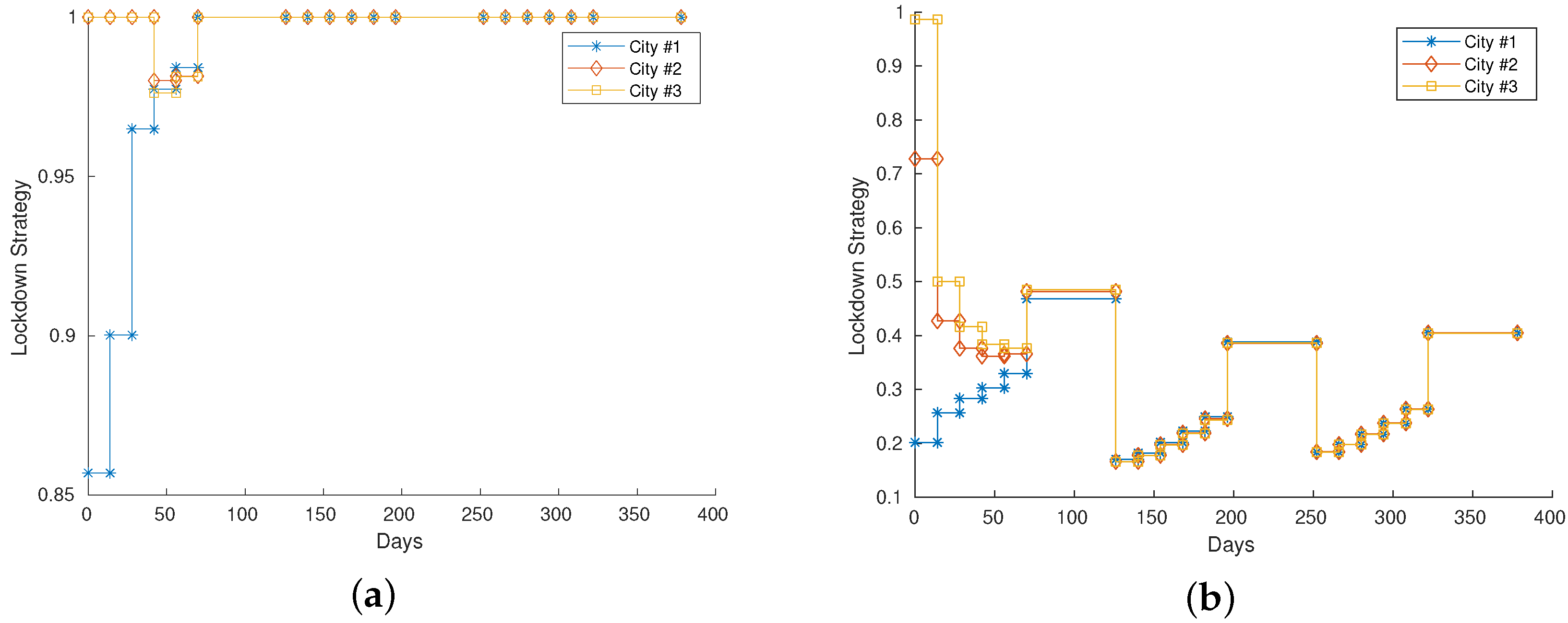
Figure 1a presents the optimized strategy for Scenario A, while Figure 1b shows the strategy for Scenario B. We have not represented the whole network but a part of it considering nodes that represent agglomerations with a different number of individuals. Furthermore, the strategy that optimizes our objective function is reproduced by showing the values of the vector $\mathit{V}$, see (6), for some cities/agglomerations present in the network. Values close to 1 mean that there are no particular restrictions on mobility, values close to 0 mean strong restrictions on movement. We point out that the value 0 is not allowed because it is not realistic to consider a total block of each movement in this context.

In the case of Scenario A, the parameter of the disease induced a light lockdown ($85\%$) on the large city (blue line), whilst the other two are almost completely open. On the second case, the disease is more infectious: the large city is forced to adopt a severe lockdown, while the strategy on the other two suggests a mild lockdown. As soon as the epidemic spreads, due to the characteristics of the disease, even the smallest cities are forced to adopt a more severe strategy until the number of infected individuals decreases. We can observe in Scenario B that, after a period of severe lockdown, when the last chosen strategy is applied for a longer period, then a further severe approach must be adopted in order to contain the epidemic.

In both scenarios, we can observe that there is a converging behavior of the strategies to be applied on the three different cities. Check, for example, the period 50–100 days in Scenario A: the lockdown strategy for the largest city (blue line) is increasing, while the strategies for the other cities (orange and yellow lines) are decreasing. Eventually, due to the disease parameters, they converge to 1, meaning that the epidemic threat is no more. This behavior is more evident in Scenario B.

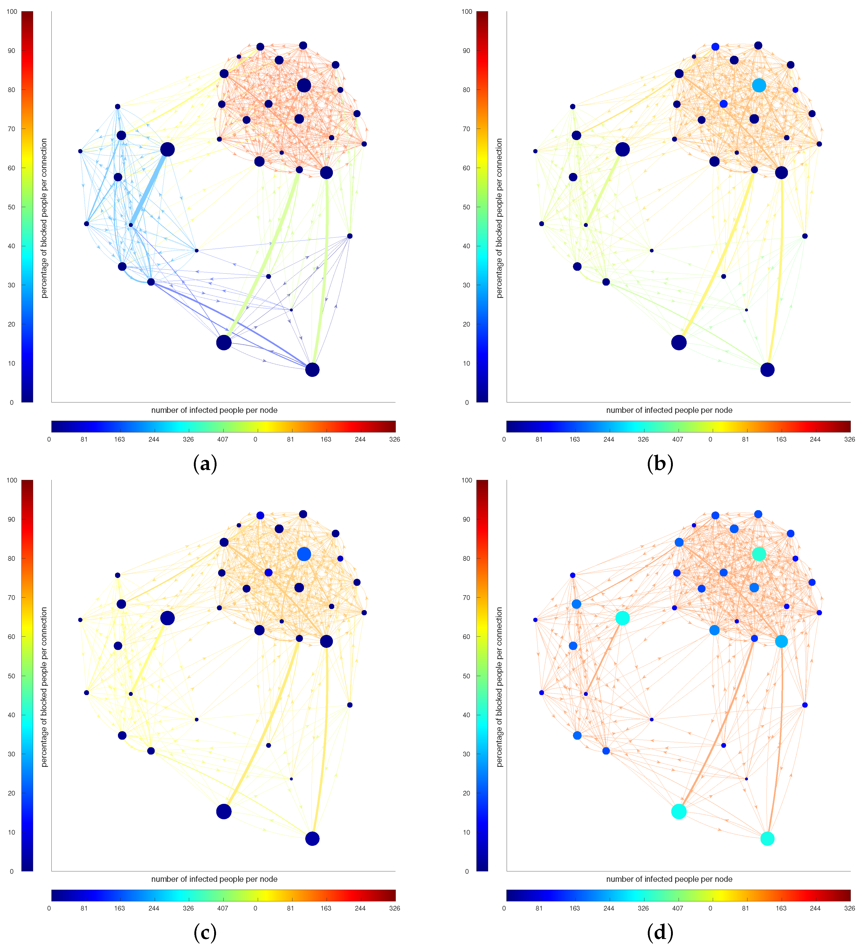
Figure 2 presents a visual representation of the evolution of the strategies for Scenario B at $t=0$, 20, 40 and 179 days. The color of the nodes represents the number of infected people in that node, while the color of the edges represents the percentage of people blocked. At the beginning, the optimal strategy suggests to mainly block the outgoing from the large city (the agglomerate on the top left corner), while the connection between and inside the other two are open. Letting the epidemic spread in a controlled way, in order to maintain economy, induces an increase in the number of infected people, then the connections between cities must be reduced (the more red the edges are, the less people are allowed to move).

4. Conclusions

The network perspective allows to relax the assumption of uniform random mixing and then we are able to model the population interaction patterns during epidemics. Moreover, a network-based model provides useful and important insights about the spread of a disease; such insights cannot be inferred using the classical model. We have focused on a SEIR meta-population model on a network in order to characterize the epidemic dynamics and to predict possible contagion scenarios.

A network model can encompass differences in the number of interactions between individuals in a population. For example, there exist some realities where people may live in small environments and they have relatively few contacts (work and/or social life), while others may live in dense and more populated centers, where the usage of public and maybe crowded public transportation is very common, they work in high-contact environments and they have a large number of interactions with many others outside of work. The classical SEIR model does not allow to include such heterogeneity, while a network model can easily encompass it. Furthermore, it is possible to adapt our model and, instead of a geographical distinction of the subgroups of individuals, different stratifications of the population can be considered.

We justified the model by introducing and analyzing some of its properties, in particular, we proved a threshold theorem involving both biological parameters and the topology of the network. In a future paper, we will consider both time-dependent parameters and a detailed analysis of the asymptotic behavior of the solution of the proposed model. We point out that our analysis can be applied to recent models, e.g., [26], where numerical and statistical but not analytical results are provided.

Only recent works, e.g., [28,29,30], started investigating the trade-off between epidemic and economic costs with some analysis. In order to take a new step in this direction, we have also identified an optimal control problem that considers the advantages and benefits that arise from the application of optimal targeted policies, which lock down the various groups in an inhomogeneous way. The focus is on the balance between economic loss and loss of life. The main economic damages consist of lost productivity due to illness and also in the forgone productivity contributions of the blocked subpopulations. The lives lost are estimated via the number of the infected individuals, assuming that these losses represent a constant percentage of the latter.

Some preliminary numerical tests are provided; more effective results could be obtained by considering a suitable fitting of the parameters and based on some particular topology of the network. These issues will be analyzed in a future paper involving a different source of data [32] and recent optimization tools [33,34].

References

- Kermack, W.O.; McKendrick, A.G.; Walker, G.T. A contribution to the mathematical theory of epidemics. Proc. R. Soc. London Ser. Contain. Pap. Math. Phys. Character 1927, 115, 700–721. [Google Scholar] [CrossRef] [Green Version]
- Anderson, R.; May, R. Infectious Diseases of Humans: Dynamics and Control; Oxford University Press: Oxford, UK, 1991. [Google Scholar]
- Hethcote, H. Mathematics of infectious diseases. SIAM Rev. 2000, 42, 599–653. [Google Scholar] [CrossRef] [Green Version]
- Capasso, V. Mathematical Structures of Epidemic Systems; Springer: Berlin/Heidelberg, Germany, 1993. [Google Scholar]
- Foppa, I. A Historical Introduction to Mathematical Modeling of Infectious Diseases: Seminal Papers in Epidemiology; Academic Press: Cambridge, MA, USA, 2016; pp. 1–197. [Google Scholar]
- Chowell, G.; Sattenspiel, L.; Bansal, S.; Viboud, C. Mathematical models to characterize early epidemic growth: A review. Phys. Life Rev. 2016, 18, 66–97. [Google Scholar] [CrossRef] [PubMed] [Green Version]
- Metcalf, C.; Lessler, J. Opportunities and challenges in modeling emerging infectious diseases. Science 2017, 357, 149–152. [Google Scholar] [CrossRef] [Green Version]
- Keeling, M.; Rohani, P. Modeling Infectious Diseases in Humans and Animals; Princeton University Press: Princeton, NJ, USA, 2011; pp. 1–368. [Google Scholar]
- Garrett, K.; Mundt, C. Epidemiology in mixed host populations. Phytopathology 1999, 89, 984–990. [Google Scholar] [CrossRef] [Green Version]
- Rimbaud, L.; Fabre, F.; Papaïx, J.; Moury, B.; Lannou, C.; Barrett, L.; Thrall, P. Models of Plant Resistance Deployment. Annu. Rev. Phytopathol. 2021, 59, 125–152. [Google Scholar] [CrossRef]
- Jeger, M.; Pautasso, M.; Holdenrieder, O.; Shaw, M. Modelling disease spread and control in networks: Implications for plant sciences. New Phytol. 2007, 174, 279–297. [Google Scholar] [CrossRef] [PubMed]
- Kenah, E.; Chao, D.; Matrajt, L.; Halloran, M.; Longini, I., Jr. The global transmission and control of influenza. PLoS ONE 2011, 6, e19515. [Google Scholar] [CrossRef] [Green Version]
- Heesterbeek, H.; Anderson, R.; Andreasen, V.; Bansal, S.; DeAngelis, D.; Dye, C.; Eames, K.; Edmunds, W.; Frost, S.; Funk, S.; et al. Modeling infectious disease dynamics in the complex landscape of global health. Science 2015, 347, aaa4339. [Google Scholar] [CrossRef] [PubMed] [Green Version]
- Nowzari, C.; Preciado, V.; Pappas, G. Analysis and Control of Epidemics: A Survey of Spreading Processes on Complex Networks. IEEE Control Syst. 2016, 36, 26–46. [Google Scholar] [CrossRef] [Green Version]
- Arino, J.; Bauch, C.; Brauer, F.; Driedger, S.; Greer, A.; Moghadas, S.; Pizzi, N.; Sander, B.; Tuite, A.; Van Den Driessche, P.; et al. Pandemic influenza: Modelling and public health perspectives. Math. Biosci. Eng. 2011, 8, 1–20. [Google Scholar] [CrossRef] [PubMed]
- Lessler, J.; Cummings, D. Mechanistic models of infectious disease and their impact on public health. Am. J. Epidemiol. 2016, 183, 415–422. [Google Scholar] [CrossRef] [PubMed]
- Masuda, N.; Miller, J.; Holme, P. Concurrency measures in the era of temporal network epidemiology: A review. J. R. Soc. Interface 2021, 18, 20210019. [Google Scholar] [CrossRef]
- Layan, M.; Dellicour, S.; Baele, G.; Cauchemez, S.; Bourhy, H. Mathematical modelling and phylodynamics for the study of dog rabies dynamics and control: A scoping review. PLoS Neglected Trop. Dis. 2021, 15, e0009449. [Google Scholar] [CrossRef] [PubMed]
- Earn, D.; Dushoff, J.; Levin, S. Ecology and evolution of the flu. Trends Ecol. Evol. 2002, 17, 334–340. [Google Scholar] [CrossRef]
- Riley, S.; Eames, K.; Isham, V.; Mollison, D.; Trapman, P. Five challenges for spatial epidemic models. Epidemics 2015, 10, 68–71. [Google Scholar] [CrossRef] [PubMed] [Green Version]
- Pellis, L.; Ball, F.; Bansal, S.; Eames, K.; House, T.; Isham, V.; Trapman, P. Eight challenges for network epidemic models. Epidemics 2015, 10, 58–62. [Google Scholar] [CrossRef]
- Miller, J.; Kiss, I. Epidemic spread in networks: Existing methods and current challenges. Math. Model. Nat. Phenom. 2014, 9, 4–42. [Google Scholar] [CrossRef] [Green Version]
- Hanski, I.; Gilpin, M. Metapopulation dynamics: Brief history and conceptual domain. Biol. J. Linn. Soc. 1991, 42, 3–16. [Google Scholar] [CrossRef]
- Hanski, I.; Gaggiotti, O. Ecology, Genetics and Evolution of Metapopulations; Academic Press: Cambridge, MA, USA, 2004; pp. 1–696. [Google Scholar] [CrossRef]
- Boccaletti, S.; Latora, V.; Moreno, Y.; Chavez, M.; Hwang, D.U. Complex networks: Structure and dynamics. Phys. Rep. 2006, 424, 175–308. [Google Scholar] [CrossRef]
- Gatto, M.; Bertuzzo, E.; Mari, L.; Miccoli, S.; Carraro, L.; Casagrandi, R.; Rinaldo, A. Spread and dynamics of the COVID-19 epidemic in Italy: Effects of emergency containment measures. Proc. Natl. Acad. Sci. USA 2020, 117, 10484–10491. [Google Scholar] [CrossRef] [PubMed] [Green Version]
- Chung, F.R.K. Spectral Graph Theory; Volume 92, CBMS Regional Conference Series in Mathematics; Published for the Conference Board of the Mathematical Sciences, Washington, DC, USA; American Mathematical Society: Providence, RI, USA, 1997; p. xii+207. [Google Scholar]
- Alvarez, F.E.; Argente, D.; Lippi, F. A Simple Planning Problem for COVID-19 Lockdown; Working Paper 26981; National Bureau of Economic Research: Cambridge, MA, USA, 2020. [Google Scholar] [CrossRef]
- Miclo, L.; Spiro, D.; Weibull, J. Optimal Epidemic Suppression under an ICU Constraint; Working Paper 1111; Toulouse School of Economics: Toulouse, France, 2020. [Google Scholar]
- Birge, J.R.; Candogan, Z.; Feng, Y. Controlling Epidemic Spread: Reducing Economic Losses with Targeted Closures; Working Paper 2020-57; Becker Frieman Institute Chicago: Chicago, IL, USA, 2020. [Google Scholar]
- Godio, A.; Pace, F.; Vergnano, A. Seir modeling of the italian epidemic of SARS-CoV-2 using computational swarm intelligence. Int. J. Environ. Res. Public Health 2020, 17, 3535. [Google Scholar] [CrossRef] [PubMed]
- Rivieccio, B.; Micheletti, A.; Maffeo, M.; Zignani, M.; Comunian, A.; Nicolussi, F.; Salini, S.; Manzi, G.; Auxilia, F.; Giudici, M.; et al. CoViD-19, learning from the past: A wavelet and cross-correlation analysis of the epidemic dynamics looking to emergency calls and Twitter trends in Italian Lombardy region. PLoS ONE 2021, 16, e0247854. [Google Scholar] [CrossRef] [PubMed]
- Zanni, L.; Benfenati, A.; Bertero, M.; Ruggiero, V. Numerical Methods for Parameter Estimation in Poisson Data Inversion. J. Math. Imaging Vis. 2015, 52, 397–413. [Google Scholar] [CrossRef]
- Benfenati, A.; Ruggiero, V. Inexact Bregman iteration with an application to Poisson data reconstruction. Inverse Probl. 2013, 29, 065016. [Google Scholar] [CrossRef] [Green Version]
Figure 1.
(a,b): Lockdown strategies for Scenario A and B, respectively. We show the optimal strategy that minimizes (7) the closer is to 0, the more severe the restrictions are. On the other hand, values close to 1 denote very mild restrictions on mobility.
Figure 2.
(a–d): Evolution of the strategy and infected people in Scenario B for timestamps , respectively. The color of the nodes represents the number of infected people in that node, while the color of the edges represents the percentage of people blocked.
Publisher’s Note: MDPI stays neutral with regard to jurisdictional claims in published maps and institutional affiliations. |
© 2021 by the authors. Licensee MDPI, Basel, Switzerland. This article is an open access article distributed under the terms and conditions of the Creative Commons Attribution (CC BY) license (https://creativecommons.org/licenses/by/4.0/).
Share and Cite
MDPI and ACS Style
Aletti, G.; Benfenati, A.; Naldi, G. Graph, Spectra, Control and Epidemics: An Example with a SEIR Model. Mathematics 2021, 9, 2987. https://0-doi-org.brum.beds.ac.uk/10.3390/math9222987
AMA Style
Aletti G, Benfenati A, Naldi G. Graph, Spectra, Control and Epidemics: An Example with a SEIR Model. Mathematics. 2021; 9(22):2987. https://0-doi-org.brum.beds.ac.uk/10.3390/math9222987
Chicago/Turabian StyleAletti, Giacomo, Alessandro Benfenati, and Giovanni Naldi. 2021. "Graph, Spectra, Control and Epidemics: An Example with a SEIR Model" Mathematics 9, no. 22: 2987. https://0-doi-org.brum.beds.ac.uk/10.3390/math9222987
Note that from the first issue of 2016, this journal uses article numbers instead of page numbers. See further details here.