Steady State and 2D Thermal Equivalence Circuit for Winding Heads—A New Modelling Approach

Abstract
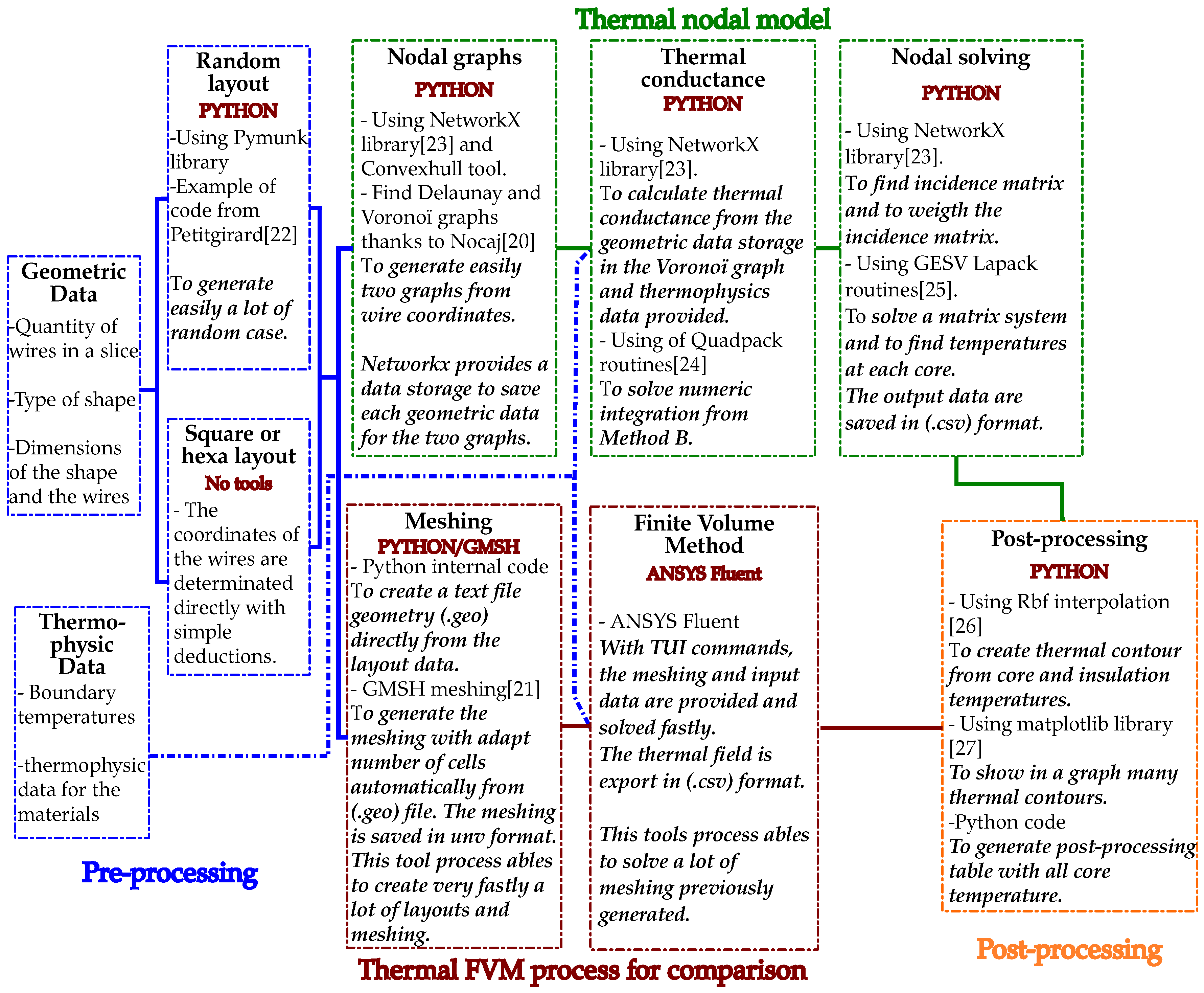
:1. Introduction
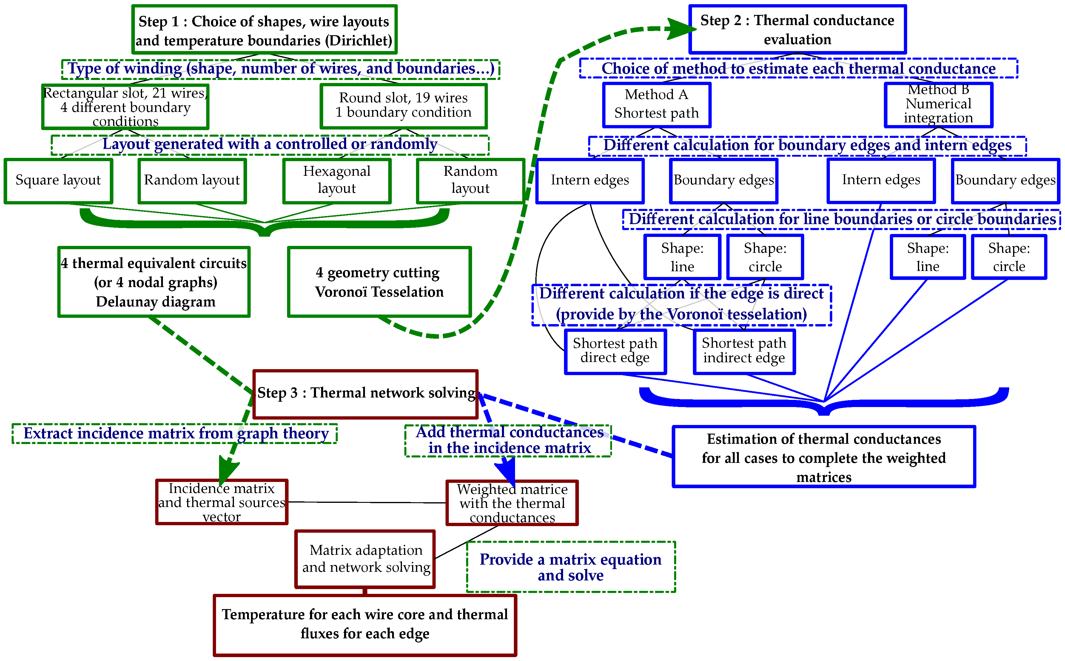
2. Thermal Equivalent Circuit
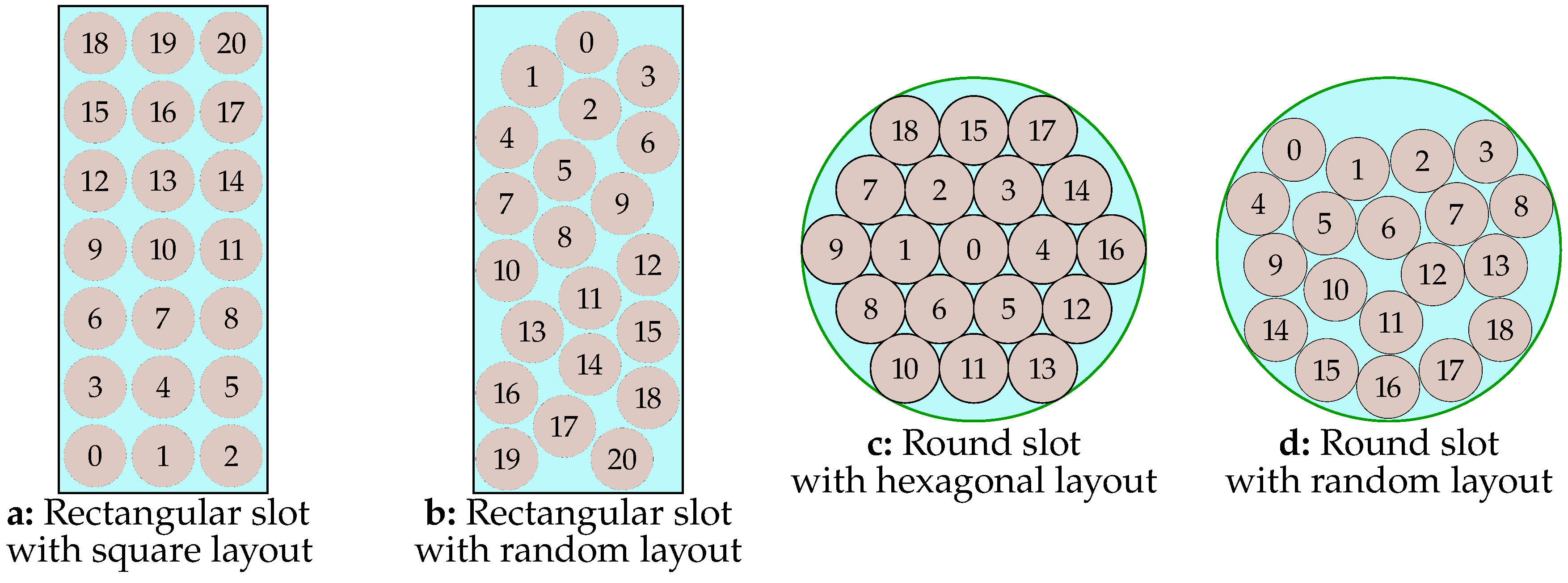
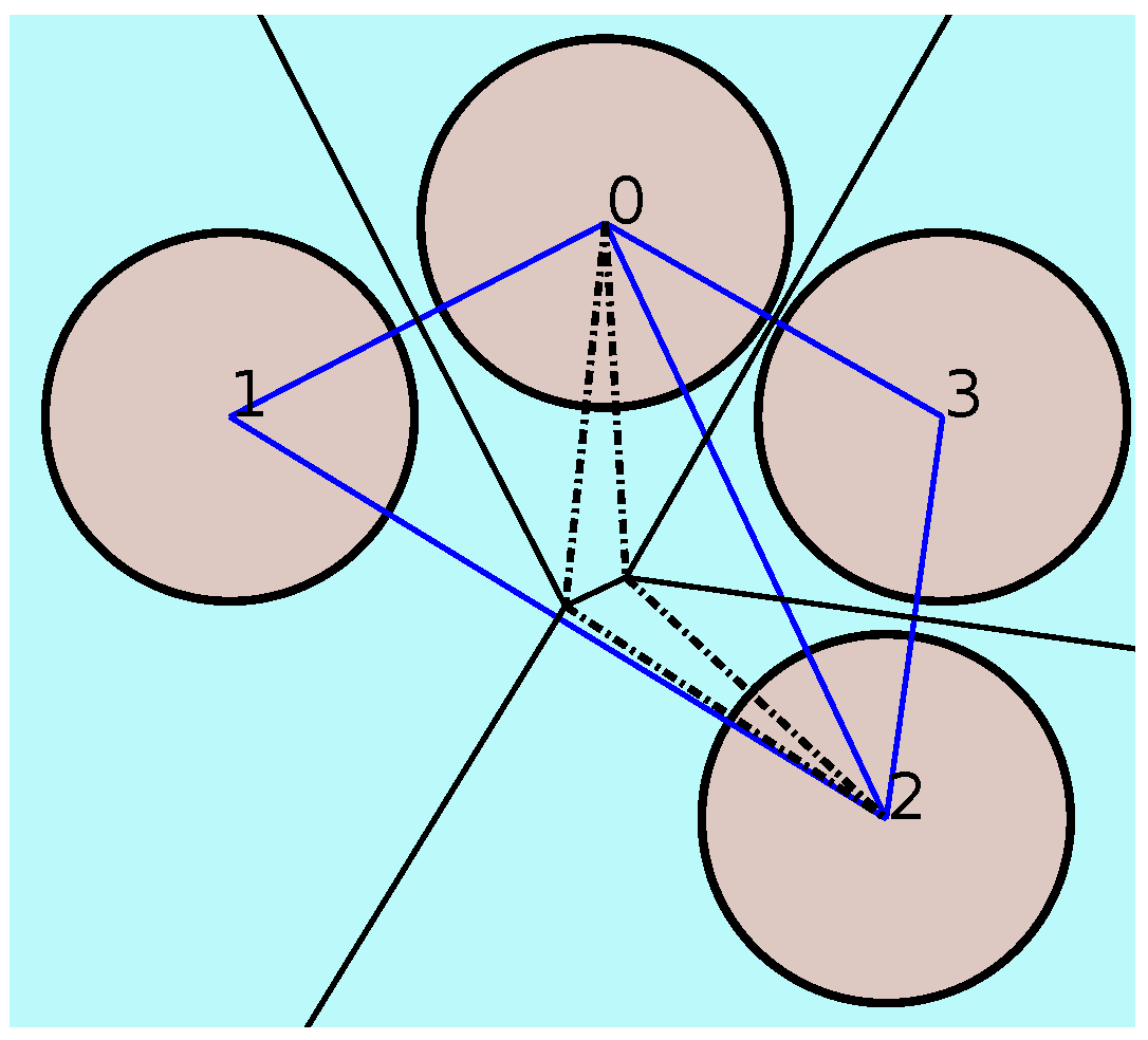
2.1. Application to a Lot of Slot Shapes with a Random Layout of Round Wires
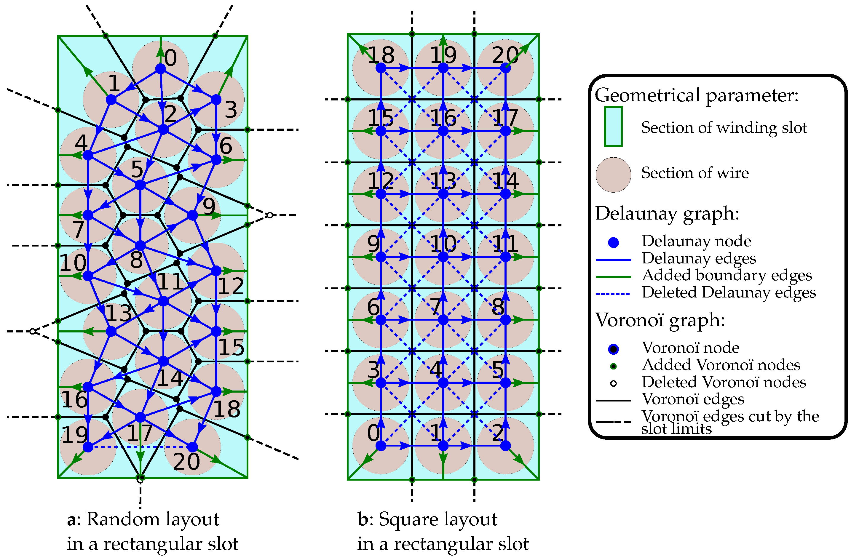
2.2. Creation of the Internal Thermal Circuit
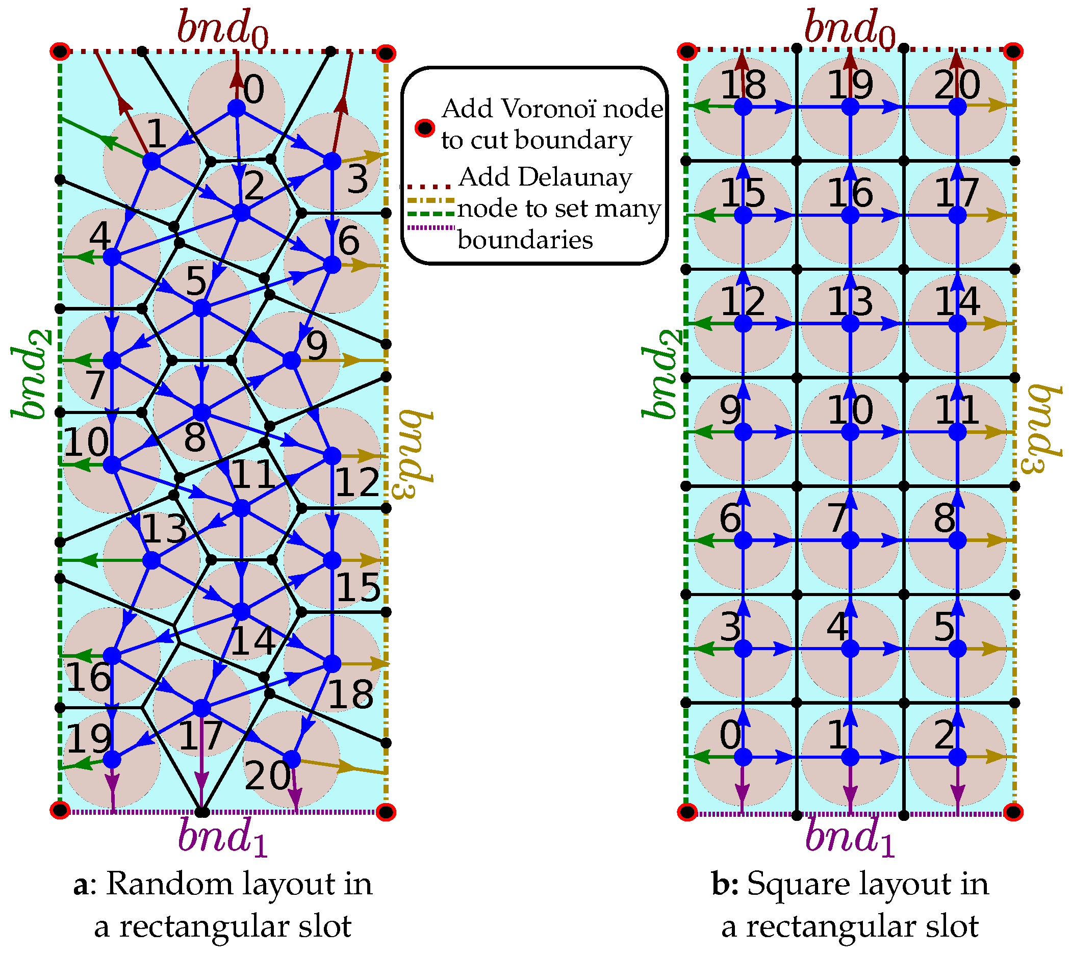
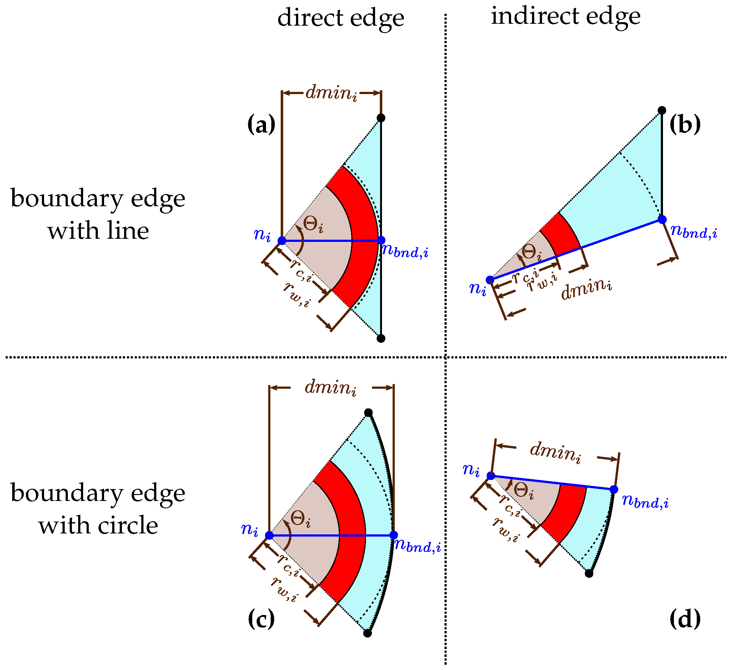
2.3. Selection of Boundary Conditions to the Thermal Circuit
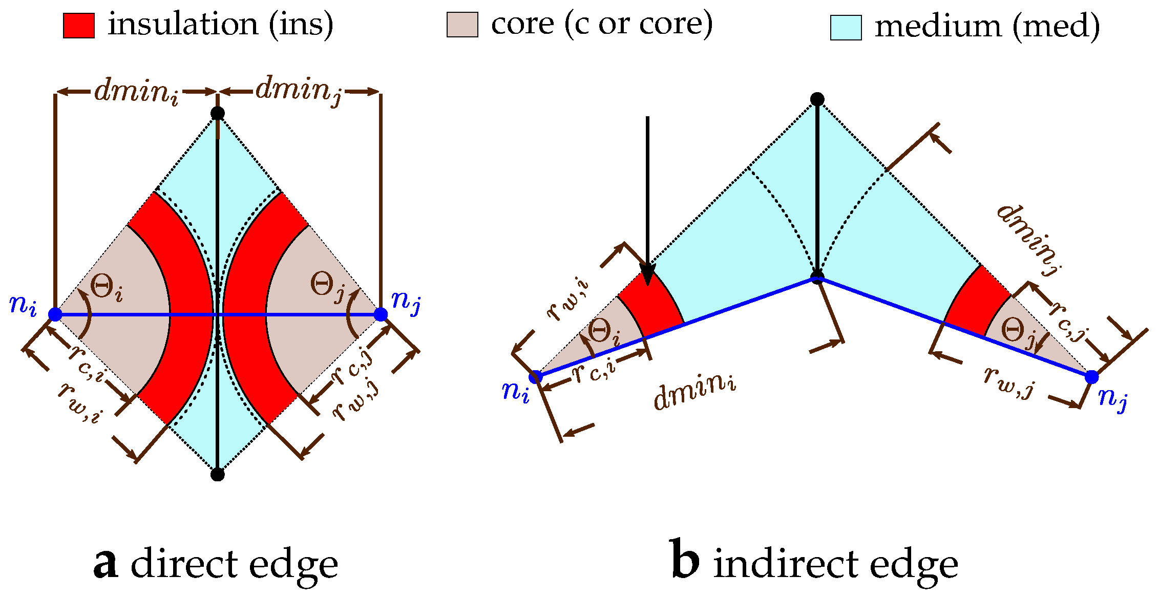
3. Thermal Conductance Determination
- A direct case when the 2 edges intersect.
- An indirect case when the 2 edges do not intersect. This case appears when the shortest distance between 2 adjacent nodes does not coincide with the Delaunay edge.
3.1. Method A: Shortest Path
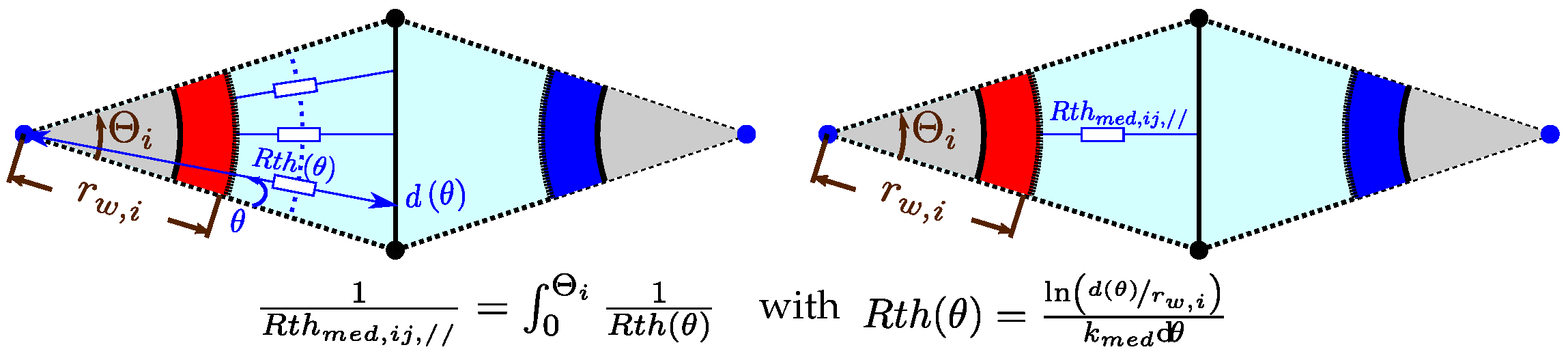
3.2. Method B: Numerical Integration
4. Nodal Network Solving


5. Application and Validation
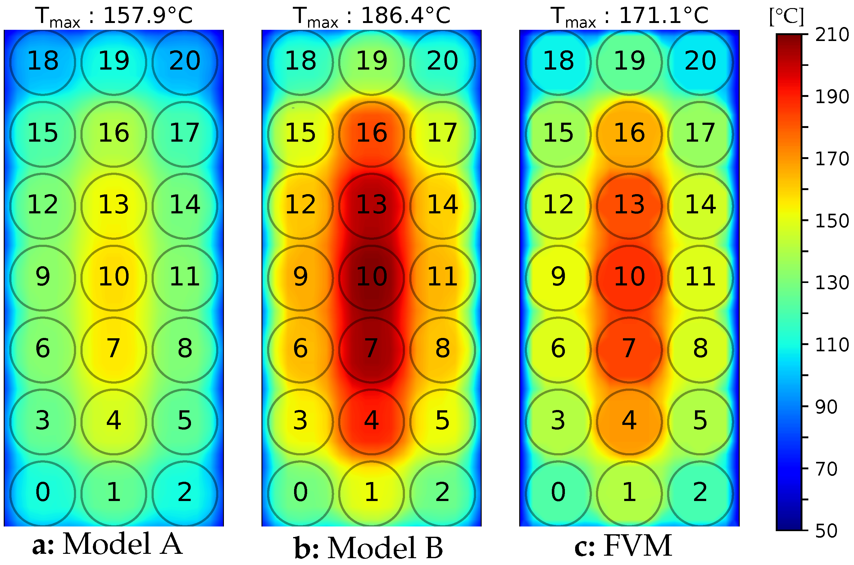
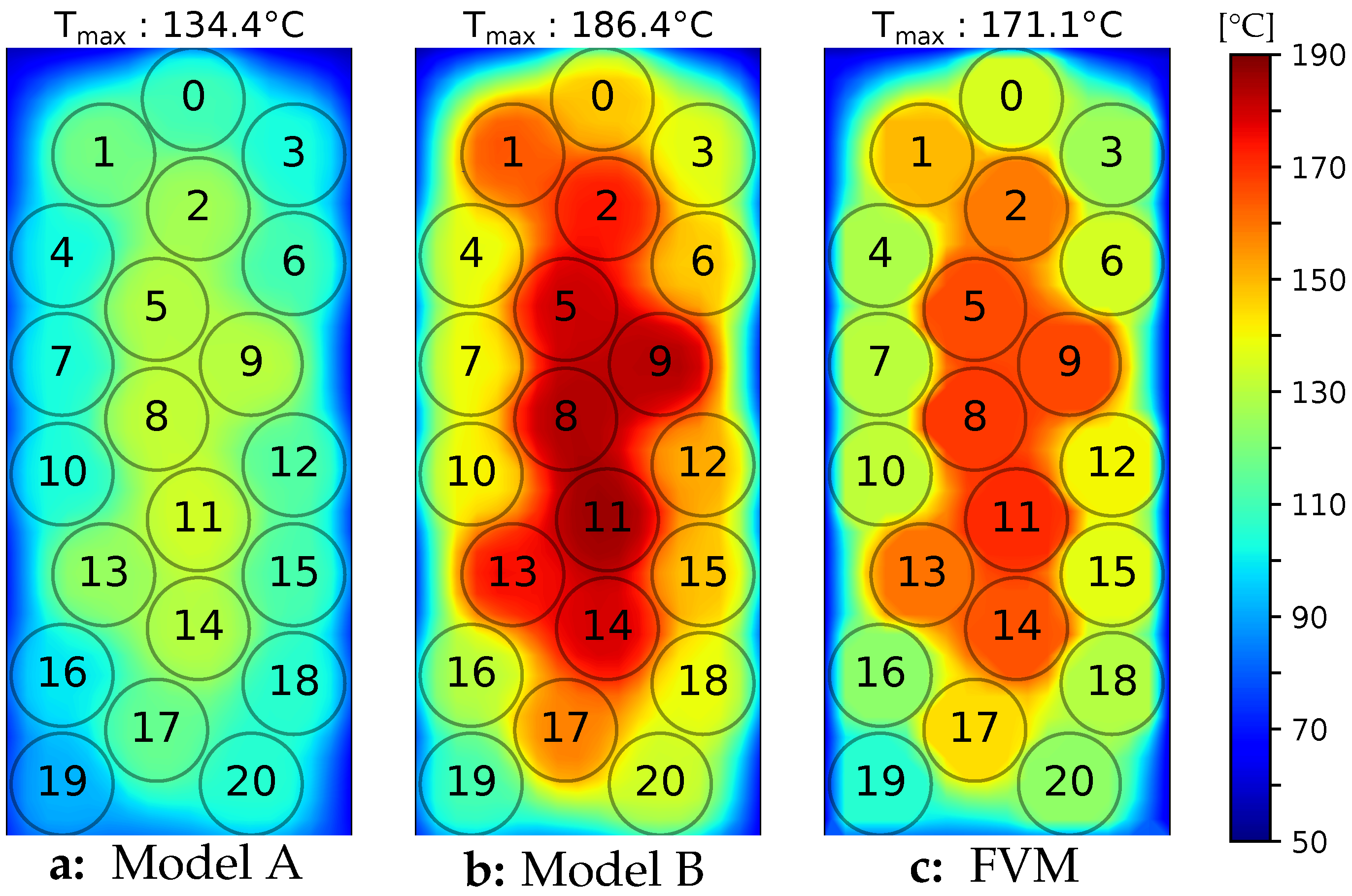
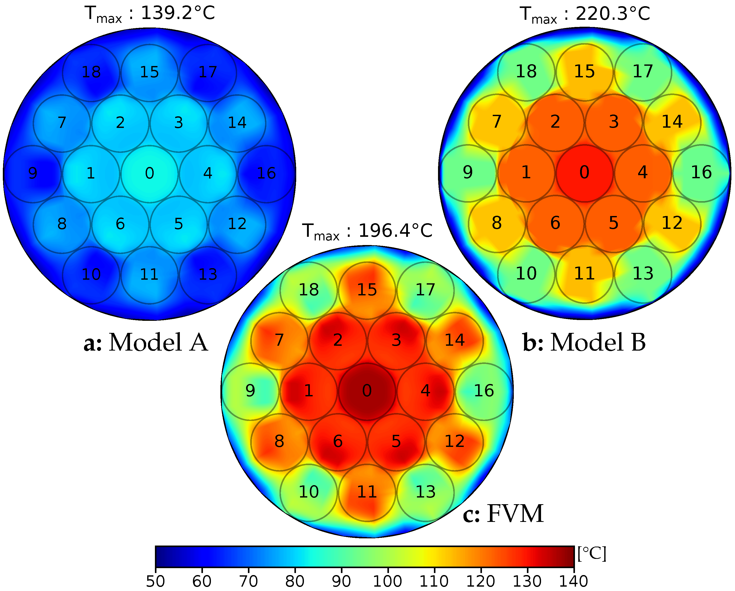
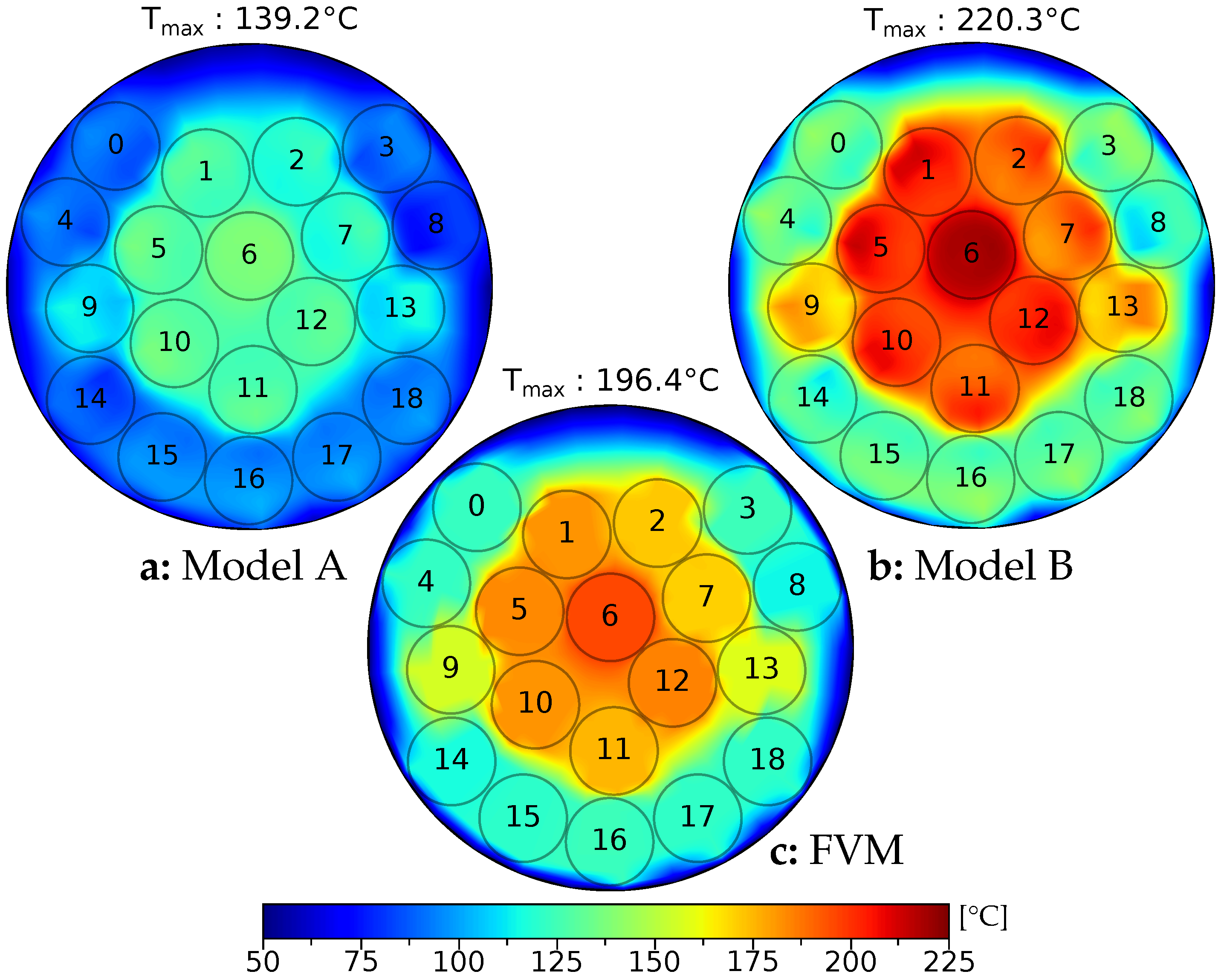
5.1. Comparison between Two Conductance Methods and a Commercial Software
5.2. Comparison between the Different Shapes and the Wire Layouts
6. Conclusions
- Add convection by using the Robin type conditions or control the outgoing heat flow at the limit with Neumann conditions.
- Refine the determination of the thermal resistance between each wire (i.e., )
- Integrate this end-winding slot model into a larger model which includes the stator.
- Thermophysical data can be made temperature dependent with an iterative convergence process in which the matrices containing the resistances and thermal conductances are updated synchronously.
- Finally, the model could be transformed into a transient model by the addition of thermal capacitors at each node.
Author Contributions
Funding
Acknowledgments
Conflicts of Interest
Appendix A. Application: Materials Properties, Dimensions and Wire Positions
Appendix A.1. Materials Properties
- Media thermal conductivity (trapped air): 0.028 W/mK
- Insulation thermal conductivity: 0.2 W/mK
- Copper electrical resistivity: m
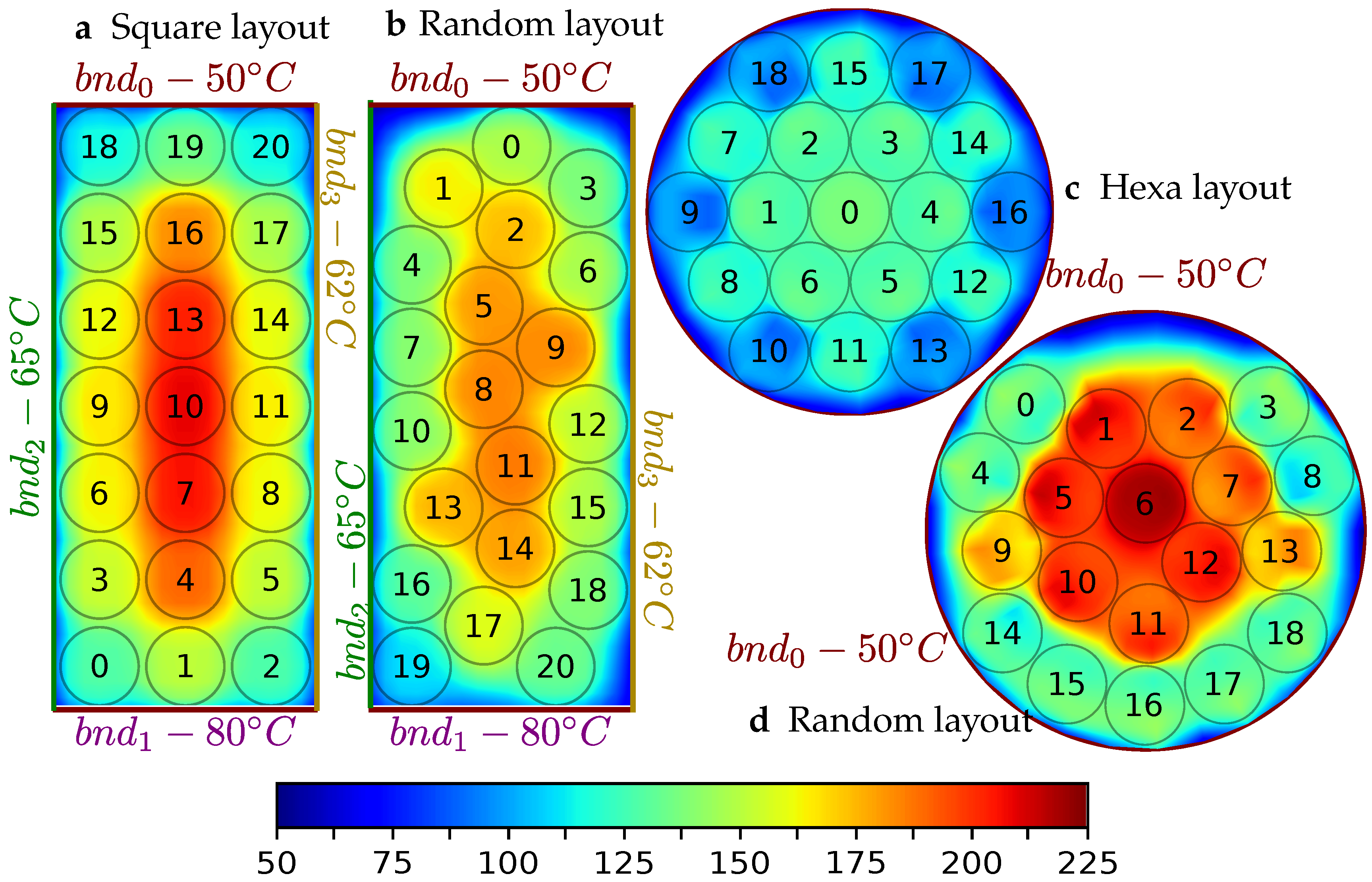
Appendix A.2. Slot Dimension, Slot Properties and Wire Positions

| Rectangular slot | Round slot | ||
|---|---|---|---|
| Figure | Figure 2a,b | Figure | Figure 2c,d |
| wire number | 21 | wire number | 19 |
| wire section | wire section | ||
| insulation thickness | insulation thickness | ||
| Surface ratio | Surface ratio | Fig. c Fig. d | |
| slot height | slot diameter | Fig. c Fig. d | |
| slot width |
| Rectangular Slot | Round Slot | |||
|---|---|---|---|---|
| position (x, y) | ||||
| Wire | Square layout | Random layout | Hexa layout | Random layout |
| 0 | () | (0.14, 3.35) | (0.0, 0.0) | (, 1.61) |
| 1 | (0.0, ) | (, 2.8) | (, 0.0) | (, 1.3) |
| 2 | (1.1, ) | (0.19, 2.27) | (, 0.888) | (0.54, 1.43) |
| 3 | () | (1.13, 2.8) | (0.512, 0.888) | (1.57, 1.58) |
| 4 | (0.0, ) | (, 1.81) | (1.025, 0.0) | (, 0.74) |
| 5 | (1.1, ) | (, 1.28) | (0.512, ) | (, 0.42) |
| 6 | () | (1.13, 1.73) | () | (0, 0.35) |
| 7 | (0.0, ) | (, 0.74) | (, 0.888) | (1.1, 0.57) |
| 8 | (1.1, ) | (, 0.2) | () | (2.14, 0.7) |
| 9 | (, 0.0) | (0.71, 0.74) | (, 0.0) | () |
| 10 | (0.0, 0.0) | () | () | () |
| 11 | (1.1, 0.0) | (0.19, ) | (0.0, ) | (0.04, ) |
| 12 | (, 1.1125) | (1.13, ) | (1.538, -0.888) | (0.71, ) |
| 13 | (0.0, 1.1125) | () | (1.025, ) | (1.73, ) |
| 14 | (1.1, 1.1125) | (0.19, ) | (1.538, 0.888) | () |
| 15 | (, 2.225) | (1.13, ) | (0.0, 1.775) | () |
| 16 | (0.0, 2.225) | () | (2.05, ) | () |
| 17 | (1.1, 2.225) | () | (1.025, 1.775) | (1,) |
| 18 | (, 3.3375) | (1.13, ) | (, 1.775) | (1.8,) |
| 19 | (0.0, 3.3375) | () | ||
| 20 | (1.1, 3.3375) | (0.71, ) | ||
Appendix B. Results Data


References
- Mellor, P.H.; Roberts, D.; Turner, D.R. Lumped parameter thermal model for electrical machines of TEFC design. IEE Proc. B Electr. Pow. Appl. 1991, 138, 205–218. [Google Scholar] [CrossRef]
- Trigeol, J.F.; Bertin, Y.; Lagonotte, P. Thermal modeling of an induction machine through the association of two numerical approaches. IEEE Trans. Energy Convers. 2006, 21, 314–323. [Google Scholar] [CrossRef]
- Fan, X.; Li, D.; Qu, R.; Wang, C. A dynamic multilayer winding thermal model for electrical machines with concentrated windings. IEEE Trans. Ind. Electron. 2019, 66, 6189–6199. [Google Scholar] [CrossRef]
- Idoughi, L.; Mininger, X.; Bouillault, F.; Bernard, L.; Hoang, E. Thermal model with winding homogenization and FIT discretization for stator slot. IEEE Trans. Magn. 2011, 47, 4822–4826. [Google Scholar] [CrossRef]
- Rasid, M.A.H.; Ospina, A.; El Kadri Benkara, K.; Lanfranchi, V. Thermal Model of Stator Slot for Small Synchronous Reluctance Machine. In Proceedings of the International Conference on Electrical Machines (ICEM), Berlin, Germany, 2–5 September 2014. [Google Scholar]
- Hoang, E.; Lécrivain, M.; Hlioui, S.; Ahmed, H.B.; Multon, B. Element of slot thermal modelling. SPEEDAM 2010, 303–305. [Google Scholar] [CrossRef]
- Dannier, A.; Pizzo, A.D.; Di Noia, L.P.; Rizzo, R. Equivalent Thermal Model of Stator Slots using FEA. In Proceedings of the 2020 IEEE Texas Power and Energy Conference (TPEC), Texas, TX, USA, 6–7 February 2020. [Google Scholar]
- Sciascera, C.; Giangrande, P.; Papini, L.; Gerada, C.; Galea, M. Analytical thermal model for fast stator winding temperature prediction. IEEE Trans. Ind. Electr. 2017, 64, 6116–6126. [Google Scholar] [CrossRef]
- Milton, G.W. Bounds on the transport and optical properties of a two-component composite material. J. Appl. Phys. 1981, 52, 5294–5304. [Google Scholar] [CrossRef]
- Hashin, Z.; Shtrikman, S. A variational approach to the theory of the elastic behaviour of multiphase materials. J. Mech. Phys. Solids 1963, 11, 127–140. [Google Scholar] [CrossRef]
- Perrins, W.T.; McKenzie, D.R.; McPhedran, R.C. Transport properties of regular arrays of cylinders. Proc. R. Soc. Lond. A Math. Phys. Eng. Sci. 1979, 369, 207–225. [Google Scholar]
- Stafford, J.; Grimes, R.; Newport, D. Development of compact thermal–fluid models at the electronic equipment level. J. Therm. Sci. Eng. Appl. 2012, 4, 031007. [Google Scholar] [CrossRef]
- Saulnier, J.B.; Alexandre, A. La modélisation thermique par la méthode nodale. Rev. Gén. Therm. 1985, 3, 363–371. [Google Scholar]
- Stenzel, P.; Dollinger, P.; Richnow, J.; Franke, J. Innovative Needle Winding Method using Curved Wire Guide in Order to Significantly Increase the Copper Fill Factor. In Proceedings of the 17th International Conference on Electrical Machines and Systems (ICEMS), Hangzhou, China, 24–25 October 2014. [Google Scholar]
- Dietz, A.; Tommaso, A.O.D.; Marignetti, F.; Miceli, R.; Nevoloso, C. Enhanced flexible algorithm for the optimization of slot filling factors in electrical machines. Energies 2020, 13, 1041. [Google Scholar] [CrossRef] [Green Version]
- Charih, F.; Dubas, F.; Espanet, C.; Bernard, R. Étude de la réduction des pertes électromagnétiques d’un MSAP à fort couple et à encoches ouvertes. In Proceedings of the Electrotechnique du Futur, Belfort, France, 14–15 December 2011. [Google Scholar]
- Incropera, F.P.; Bergman, T.L.; DeWitt, D.P.; Lavine, A.S. Free Convection. In Fundamentals of Heat and Mass Transfer; Wiley: Hoboken, NJ, USA, 2013. [Google Scholar]
- Delaunay, B. Sur la sphère vide. À la mémoire de Georges Voronoï. Bulletin de l’Académie des Sciences de l’URSS. Classe des Sciences Mathématiques et Naturelles. Available online: http://mi.mathnet.ru/eng/izv4937 (accessed on 16 October 2020).
- Szabó, P.G.; Markót, M.C.; Csendes, T.; Specht, E.; Casado, L.G. New Approaches to Circle Packing in a Square; Springer-Verlag GmbH: Wien, Austria, 2007. [Google Scholar]
- Nocaj, A.; Brandes, U. Computing Voronoi Treemaps: Faster, Simpler, and Resolution-independent. Comput. Gr. Forum 2012, 31, 855–864. [Google Scholar] [CrossRef] [Green Version]
- Geuzaine, C.; Remacle, J.F. Gmsh: A 3-D finite element mesh generator with built-in pre- and post-processing facilities. Int. J. Numer. Method. Eng. 2009, 79, 1309–1331. [Google Scholar] [CrossRef]
- Petitgirard, J.; Baucour, P.; Chamagne, D.; Fouillien, E. Étude 2D de l’échauffement d’un faisceau électrique pour une multitude de dispositions aléatoires de fils. Available online: https://www.sft.asso.fr/actes.html (accessed on 16 October 2020).
- Hagberg, A.A.; Schult, D.A.; Swart, P.J. Exploring Network Structure, Dynamics, and Function Using NetworkX. In Proceedings of the 7th Python in Science Conference, Pasadena, CA, USA, 19–24 August 2008. [Google Scholar]
- Piessens, R.; de Doncker-Kapenga, E.; Überhuber, C.W.; Kahaner, D.K. Quadpack; Springer: Heidelberg, Germany, 1983. [Google Scholar]
- Anderson, E.; Bai, Z.; Bischof, C.; Blackford, S.; Demmel, J.; Dongarra, J.; Du Croz, J.; Greenbaum, A.; Hammarling, S.; McKenney, A.; et al. LAPACK Users’ Guide, 3rd ed.; Society for Industrial and Applied Mathematics: Philadelphia, PA, USA, 1999. [Google Scholar]
- Buhmann, M.D. Radial Basis Functions: Theory and Implementations; Cambridge University Press: London, UK, 2003. [Google Scholar]
- Hunter, J.D. Matplotlib: A 2D graphics environment. Comput. Sci. Eng. 2007, 9, 90–95. [Google Scholar] [CrossRef]


| Square Layout in Rectangular Slot cf. Figure 2a | Random Layout in Rectangular Slot cf. Figure 2b | ||||||||||
|---|---|---|---|---|---|---|---|---|---|---|---|
| T [C] | Model A | Model B | FVM | T [C] | Model A | Model B | FVM | ||||
| 110.9 | 127.7 | 121.5 | % | 8.6% | 109.0 | 146.3 | 135.5 | % | 12.7% | ||
| 125.2 | 150.5 | 140.6 | % | 10.9% | 117.9 | 162.8 | 149.7 | % | 13.2% | ||
| 109.7 | 126.5 | 119.7 | % | 9.8% | 126.2 | 173.1 | 159.2 | % | 12.7% | ||
| 125.8 | 153.2 | 140.8 | % | 13.6% | 102.8 | 136.4 | 126.2 | % | 13.5% | ||
| 147.0 | 189.4 | 168.9 | % | 17.2% | 102.4 | 137.7 | 128.4 | % | 11.9% | ||
| 124.4 | 151.6 | 139.9 | % | 13.1% | 129.4 | 180.1 | 166.1 | % | 12.0% | ||
| 131.7 | 162.9 | 148.6 | % | 14.5% | 109.7 | 146.3 | 135.2 | % | 13.0% | ||
| 155.5 | 204.6 | 183.9 | % | 15.5% | 103.5 | 139.6 | 130.4 | % | 11.4% | ||
| 130.1 | 161.2 | 148.1 | % | 13.4% | 131.6 | 183.2 | 168.6 | % | 12.4% | ||
| 132.8 | 165,0 | 151.4 | % | 13.5% | 129.7 | 182.1 | 166.6 | % | 13.3% | ||
| 157.1 | 207.9 | 187,0 | % | 15.2% | 103.9 | 140.4 | 131.4 | % | 11.1% | ||
| 131.2 | 163.3 | 149.2 | % | 14.3% | 133.8 | 185.4 | 171.1 | % | 11.8% | ||
| 129.9 | 161.2 | 147.9 | % | 13.6% | 112.9 | 151.2 | 140.4 | % | 12.0% | ||
| 152.0 | 202.0 | 181.7 | % | 15.4% | 124.0 | 174.3 | 160.4 | % | 12.6% | ||
| 128.3 | 159.5 | 146.4 | % | 13.6% | 129.4 | 178.5 | 164.8 | % | 12.0% | ||
| 120.9 | 148.3 | 137.1 | % | 12.9% | 111.1 | 147.8 | 137.9 | % | 11.2% | ||
| 140.1 | 182.3 | 165.9 | % | 14.2% | 99.4 | 130.1 | 122.9 | % | 9.9% | ||
| 119.4 | 146.7 | 135,0 | % | 13.7% | 116.1 | 157.2 | 144.7 | % | 13.2% | ||
| 98.6 | 114.9 | 108.4 | % | 11.2% | 105.5 | 138.2 | 129.9 | % | 10.5% | ||
| 109.7 | 133.9 | 124.8 | % | 12.2% | 91.7 | 110.5 | 105.7 | % | 8.5% | ||
| 97.4 | 113.7 | 106.9 | % | 11.9% | 104.8 | 133.1 | 123.7 | % | 12.7% | ||
| 50.0 | 50.0 | ||||||||||
| 80.0 | 80.0 | ||||||||||
| 65 | 65 | ||||||||||
| 62 | 62 | ||||||||||
| [A] | 7.5 | [A] | 7.5 | ||||||||
| [W] | 13.15 | [W] | 13.15 | ||||||||
| Hexa. Layout in Round Slot cf. Figure 2c | Random Layout in Round Slot cf. Figure 2d | ||||||||||
|---|---|---|---|---|---|---|---|---|---|---|---|
| T [C] | Model A | Model B | FVM | T [C] | Model A | Model B | FVM | ||||
| 81.9 | 134.2 | 129.7 | % | 5.6% | 90.3 | 132.0 | 122.6 | % | 13.0% | ||
| 78.5 | 127.1 | 122.7 | % | 6.1% | 124.5 | 198.7 | 181.7 | % | 12.9% | ||
| 78.5 | 127.2 | 122.9 | % | 5.9% | 117.4 | 187.2 | 171.7 | % | 12.7% | ||
| 78.5 | 127.2 | 122.9 | % | 5.9% | 90.5 | 133.6 | 123.8 | % | 13.2% | ||
| 78.5 | 127.1 | 122.9 | % | 5.8% | 90.8 | 131.7 | 122.2 | % | 13.2% | ||
| 78.5 | 127.2 | 122.9 | % | 5.8% | 127.4 | 198.6 | 183.1 | % | 11.6% | ||
| 78.5 | 127.2 | 122.8 | % | 6.0% | 134.4 | 212.3 | 195.9 | % | 11.2% | ||
| 73.7 | 117.7 | 113.4 | % | 6.9% | 117.7 | 184.4 | 170.6 | % | 11.4% | ||
| 73.7 | 117.7 | 113.2 | % | 7.1% | 81.5 | 122.7 | 114.7 | % | 12.4% | ||
| 64.2 | 96.2 | 93.3 | % | 6.7% | 109.1 | 169.2 | 156.1 | % | 12.4% | ||
| 64.5 | 96.7 | 93.7 | % | 7.0% | 128.1 | 195.2 | 181.0 | % | 10.8% | ||
| 74.0 | 118.1 | 113.7 | % | 7.0% | 125.0 | 188.5 | 174.9 | % | 10.9% | ||
| 73.7 | 117.7 | 113.3 | % | 6.9% | 127.2 | 199.4 | 184.2 | % | 11.3% | ||
| 64.5 | 96.7 | 93.7 | % | 7.0% | 110.1 | 171.4 | 158.0 | % | 12.4% | ||
| 73.7 | 117.7 | 113.5 | % | 6.7% | 87.0 | 124.6 | 116.4 | % | 12.4% | ||
| 74.0 | 118.1 | 113.7 | % | 6.9% | 93.7 | 129.4 | 121.0 | % | 11.9% | ||
| 64.2 | 96.2 | 93.3 | % | 6.9% | 96.1 | 132.6 | 123.7 | % | 12.2% | ||
| 64.5 | 96.7 | 93.7 | % | 7.0% | 94.8 | 129.9 | 121.3 | % | 12.1% | ||
| 64.5 | 96.7 | 93.7 | % | 6.9% | 93.4 | 130.0 | 121.2 | % | 12.4% | ||
| 50.0 | 50.0 | ||||||||||
| [A] | 7.5 | [A] | 7.5 | ||||||||
| [W] | 13.15 | [W] | 13.15 | ||||||||
Publisher’s Note: MDPI stays neutral with regard to jurisdictional claims in published maps and institutional affiliations. |
© 2020 by the authors. Licensee MDPI, Basel, Switzerland. This article is an open access article distributed under the terms and conditions of the Creative Commons Attribution (CC BY) license (http://creativecommons.org/licenses/by/4.0/).
Share and Cite
Petitgirard, J.; Piguet, T.; Baucour, P.; Chamagne, D.; Fouillien, E.; Delmare, J.-C. Steady State and 2D Thermal Equivalence Circuit for Winding Heads—A New Modelling Approach. Math. Comput. Appl. 2020, 25, 70. https://0-doi-org.brum.beds.ac.uk/10.3390/mca25040070
Petitgirard J, Piguet T, Baucour P, Chamagne D, Fouillien E, Delmare J-C. Steady State and 2D Thermal Equivalence Circuit for Winding Heads—A New Modelling Approach. Mathematical and Computational Applications. 2020; 25(4):70. https://0-doi-org.brum.beds.ac.uk/10.3390/mca25040070
Chicago/Turabian StylePetitgirard, Julien, Tony Piguet, Philippe Baucour, Didier Chamagne, Eric Fouillien, and Jean-Christophe Delmare. 2020. "Steady State and 2D Thermal Equivalence Circuit for Winding Heads—A New Modelling Approach" Mathematical and Computational Applications 25, no. 4: 70. https://0-doi-org.brum.beds.ac.uk/10.3390/mca25040070