The Pareto Tracer for General Inequality Constrained Multi-Objective Optimization Problems


1
Computer Science Department, Cinvestav-IPN, 07360 Mexico City, Mexico
2
ESFM, Instituto Politécnico Nacional, 07738 Mexico City, Mexico
*
Author to whom correspondence should be addressed.
Math. Comput. Appl. 2020, 25(4), 80; https://0-doi-org.brum.beds.ac.uk/10.3390/mca25040080
Submission received: 22 October 2020
/
Revised: 12 December 2020
/
Accepted: 18 December 2020
/
Published: 20 December 2020
(This article belongs to the Special Issue Numerical and Evolutionary Optimization 2020)
Abstract
:Problems where several incommensurable objectives have to be optimized concurrently arise in many engineering and financial applications. Continuation methods for the treatment of such multi-objective optimization methods (MOPs) are very efficient if all objectives are continuous since in that case one can expect that the solution set forms at least locally a manifold. Recently, the Pareto Tracer (PT) has been proposed, which is such a multi-objective continuation method. While the method works reliably for MOPs with box and equality constraints, no strategy has been proposed yet to adequately treat general inequalities, which we address in this work. We formulate the extension of the PT and present numerical results on some selected benchmark problems. The results indicate that the new method can indeed handle general MOPs, which greatly enhances its applicability.
1. Introduction
In many real-world applications, the problem occurs that several conflicting and incommensurable objectives have to be optimized concurrently. As general example, in the design of basically any product, both cost (to be minimized) and quality (to be maximized) are relevant objectives, among others. Problems of that kind are termed multi-objective optimization problems (MOPs). In the case all of the objectives are continuous and in conflict with each other, it is known that there is not one single solution to be expected (as it is the case for scalar optimization problems, i.e., problems where one objective is considered) but an entire set of solutions. More precisely, one can expect that the solution set—the Pareto set, and, respectively its image, the Pareto front—forms at least locally an object of dimension , where k is the number of objectives involved in the problem. Due to this, “curse of dimensionality” problems with more than, e.g., four objectives are also called many objective optimization problems (MaOPs).
In the literature, many different methods for the numerical treatment of MOPs and MaOPs can be found (see also the discussion in the next section). One class of such methods is given by specialized continuation methods that take advantage of the fact that the solution set forms—at least locally and under certain mild assumption on the model as discussed in [1]—a manifold. Continuation methods start with one (approximate) solution of the problem and perform a movement along the Pareto set/front of the given M(a)OP via considering the underdetermined system of equations that is developed out of the Karush–Kuhn–Tucker (KKT) equations of the problem. By construction, continuation methods are of local nature. That is, if the Pareto set consists of different connected components, such methods will have to be fed with several starting points in order to obtain approximations of the entire solution set. On the other hand, continuation methods are probably most effective locally (i.e., within each connected component). Thus far, several multi-objective continuation methods have been proposed. Most of these continuation methods, however, are designed for or restricted to the treatment of bi-objective problems (i.e., MOPs with two objectives). The method of Hillermeier [1] and the Pareto Tracer (PT [2]) have been proposed for general number k of objectives. The method of Hillermeier is applicable to unconstrained and equality constrained MOPs, and the PT in addition to box constrained problems. Thus far, no extensions for these two methods are known for the treatment of general inequalities, which represents a significant shortcoming since such constraints naturally arise in many applications (e.g., [3,4]). In this paper, we extend the PT for the treatment of general inequality constraints. To this end, we utilize and adapt elements from active set methods to decide which of the inequalities have to be treated as equalities at each candidate solution. We demonstrate the strength of the novel algorithm on several benchmark test functions and present comparisons to some other numerical multi-objective solvers. The results indicate that the new method can indeed reliably handle MOPs with general constraints.
The remainder of this paper is organized as follows. In Section 2, we shortly present the required background for the understanding of this work. In Section 3, we adapt the Pareto Tracer for the treatment of general (equality and inequality) constraints. In Section 4, we present some results of the PT as well as some other multi-objective numerical methods on selected benchmark problems. Finally, we draw our conclusions in Section 5 and give possible paths for future research.
2. Background and Related Work
In this section, we briefly state the main concepts and notations that are used for the understanding of this work (for details, we refer to, e.g., [5,6]).
We consider here continuous multi-objective optimization problem (MOPs) that can be defined mathematically as
where , is the map of the k individual objectives . We assume that all objectives and constraint functions are twice continuously differentiable. The domain Q of the functions is defined by the equality and inequality constraints of (1):
If a point satisfies all constraints of (1), i.e., if , we call this point feasible. Points are called infeasible. If objectives are considered, the problem is also termed a bi-objective optimization problem (BOP).
We say that a point dominates a point (in short: ) if for all , and there exists an index j such that . A point is called Pareto optimal or simply optimal if there does not exist a vector that dominates . A point is called locally optimal if there does not exist a vector that dominates , where is a neighborhood of . The set of all Pareto optimal solutions is called the Pareto set, and its image the Pareto front. In [1], it has been shown that one can expect that both Pareto set and front typically form ()-dimensional objects under certain (mild) conditions on the problem.
If all objectives and constraint functions are differentiable, local optimal solutions can be characterized by the Karush–Kuhn–Tucker (KKT) equations [7,8]:
Theorem 1.
Suppose that is locally optimal with respect to (1). Then, there exist Lagrange multipliers , and such that the following conditions are satisfied
Multi-objective optimization is an active field of research, and thus far many numerical methods have been proposed for the treatment of such problems. There exist for instance many methods that are designed to compute single solutions such as the weighted sum method [9], the -constraint method [5,10], the weighted metric and weighted Tchebycheff method [5,11,12], as well as reference point problems [13,14,15]. All of these methods transform the given MOP into a scalar optimization problem (SOP) that can to a certain extent to include users’ preferences. These methods can either be used as standalone algorithm (i.e., for the computation of single solutions) or be used to obtain a finite size approximation of the entire Pareto set/front of the given MOP via utilizing a clever sequence of these SOPs [5,16,17,18,19].
Further, there exist set oriented methods such as cell mapping techniques [20,21,22,23]), subdivision techniques [24,25,26,27], and multi-objective evolutionary algorithms (MOEAs, e.g., [3,28,29,30,31,32,33,34]). All of these methods manipulate an entire set of candidate solutions in each iteration and hence yield a finite size approximation of the solution set in one run of the algorithm. Hybridizations of such techniques with mathematical programming techniques can be found in [31,35,36,37,38,39,40,41].
Finally, a third class of numerical solvers for MOPs is given by specialized continuation methods that take advantage of the fact that the Pareto set/front of a given problem forms at least locally a manifold of a certain dimension. Methods of this kind start with a given (approximate) solution and perform a movement along the Pareto set/front of the problem. The first such method is proposed in [1], which can be applied to unconstrained and equality constrained MOPs of any number k of objectives, while no strategies are reported on how to treat inequalities. ParCont [42,43] is a rigorous predictor–corrector method that is based on interval analysis and parallelotope domains. The method can deal with equality and inequality constraints, but it is restricted to bi-objective problems. This restriction also holds for the method presented in [44], which has been designed to provide an equispaced approximation of the Pareto front. The Zigzag method [45,46,47] obtains Pareto front approximations via alternating optimizing one of the objectives. This approach is also limited to the treatment of bi-objective problems.
In [48], a continuation method is presented that is applicable to box-constrained BOPs. In [49], a variant of the method of Hillermeier is presented that is designed for the treatment of high-dimensional problems.
Recently, the Pareto Tracer (PT) was proposed by Martin and Schütze [2]. Similar to the method of Hillermeier, PT addresses the underdetermined nonlinear system of equations that is induced by the KKT equations. However, unlike the method of Hillermeier, the PT aims to separate the decision variables from the associated weight (or Lagrange) vectors whenever possible, leading to significant changes. The latter is due to the fact that the nonlinearity of the equation system can be significantly higher in the compound space compared to the corresponding system that is only defined in decision variable space. As a by-product, the chosen approach allows to compute the tangent space of both Pareto set and front at every given regular point x. In [50], elements of the PT are used to treat many objective optimization problems (i.e., MOPs with more than, e.g., five objectives). Thus far, PT is only applicable to box and equality constrained problems which limits its application. In the following, we propose and discuss an extension of this method to adequately treat general MOPs, i.e., MOPs that in particular contain general inequalities.
3. Adapting the Pareto Tracer for General Inequality Constrained MOPs
In this section, we adapt the PT so that is can handle general inequality constraints. The core is the predictor–corrector step that generates from a given candidate solution the following candidate that satisfies the KKT conditions, and so that defines a pre-described movement in objective space along the set of KKT points.
Assume we are given a MOP of form (1) and a feasible point that satisfies the KKT conditions (3), where , . Let and define by
the set of indices corresponding to the nearly active inequalities at . If , , define
Further, let
and , , and be the solution of
Note that (7) yields the Lagrange multipliers at for if is a KKT point and if all active inequalities are regarded as equalities. Using , and , define the matrix
To compute a predictor direction , we solve the the system
Note that system (9) depends on . Before we specify this vector, we first simplify (9). Denote by
then (9) is equivalent to
Let . It is straightforward to show that for a vector that solves (11), where is chosen such that
it holds
That is, (infinitesimal) small steps from into direction (in decision variable space) will lead to a movement from into direction d (in objective space). It remains to select a suitable choice for d. Since is orthogonal to the linearized Pareto front at [1], a suggesting choice is hence by (13) to take d orthogonal to . For this, let
where is orthogonal and , be a -factorization of . Then, any vector
can be chosen so that a movement in direction (in decision variable space) leads to a movement from along the Pareto front. Note that the second equation in (12) reads as . Hence, for the special case of a bi-objective optimization problem (i.e., ), there are—after normalization—only two choices for :
Analog to Martin and Schütze [2], one can show that corresponds to a “right down” movement along the Pareto front while corresponds to a "left up" movement along the Pareto front.
After selecting the predictor direction , the question is how far to step in this direction. Here, we follow the suggestion made by Hillermeier [1] and use the step size
for a (small) value so that
For the computations presented below, we make the following modifications: instead of , we use the matrix
More precisely, for the computation of , we use the system
and to obtain we solve
We have observed similar performance for both approaches, while the usage of compared to comes with the advantage that no Hessians for any of the constraint functions have to be computed.
Given a predictor point
the task of the upcoming corrector step is to find a KKT point that is ideally near to . For this, we suggest to apply the multi-objective Newton method proposed in [51]. In particular, we first compute the solution of the following problem
is indeed the Newton direction for equality constrained MOPs as suggested in [2]. To adequately treat the involved inequalities, however, we propose to use the solution of the following problem:
Note that problem is identical to problem except that inequalities are treated as equalities at . In particular, we propose to add an index i to if
- (a)
- , i.e., if significantly violates the constraint ; or
- (b)
- and , i.e., if is either active but nearly active at or if already slightly violates and a step into direction would lead to (further) violation of this constraint, indicated by .
Algorithm 1 shows the pseudo code to build the index set at a predictor point . Given the Newton direction, the Newton step can then be performed via using the Armijo rule described in [51], as done in our computations. The set is only computed once, it and remains fixed during the Newton iteration in the corrector step.
Algorithm 2 shows the pseudo code of one predictor–corrector step of the PT for general (equality and inequality constrained) MOPs. For bi-objective problems, can be chosen as in (16) leading either to a “left up” or “right down” movement, as discussed above. The algorithm has to be stopped if is either close enough to or , depending of course on the chosen search direction. For , one can use the box partition in objective space as described in [2] in order to mark the regions of the Pareto front that have already been “covered” during the run of the algorithm.
For the realization of the predictor–corrector step several linear systems of equations have to be solved, the largest one being (20). The cost is hence in terms of flops and in terms of storage. Further, for the corrector step the SOP (7) has to be solved that contains decision variables. For the computation of the Newton direction, the SOPs (23) and (24) have to be solved for the first Newton iteration that contains both decision variables. For further Newton iterations, only SOP (24) has to be solved since the index set remains fixed within a corrector step. Finally, note that, if the method is realized as described above, the Hessians of all individual objectives have to be computed at each candidate solution (including at each Newton iteration). Using ideas from quasi-Newton methods, one can approximate the Hessians so that only gradient information is needed at each candidate solution, as described in [2].
| Algorithm 1 Build |
| Require:: predictor, : corrector direction for , : tolerance Ensure:: index set 1: 2: fordo 3: ifthen 4: 5: else ifthen 6: 7: end if 8: end for 9: Return |
| Algorithm 2 Predictor–corrector step of the Pareto Tracer for general MOPs |
| Require:: current candidate solution, : desired distance in objective space, : tolerance Ensure:: new candidate solution 1: Compute via solving (7) 2: Compute as in (19) 3: Compute A as in (10) 4: Select as in (16) or via (15) and (21) 5: Compute via solving (20) 6: 7: 8: Compute via a Newton method starting at . For the Newton direction use the solution of (24). 9: Return |
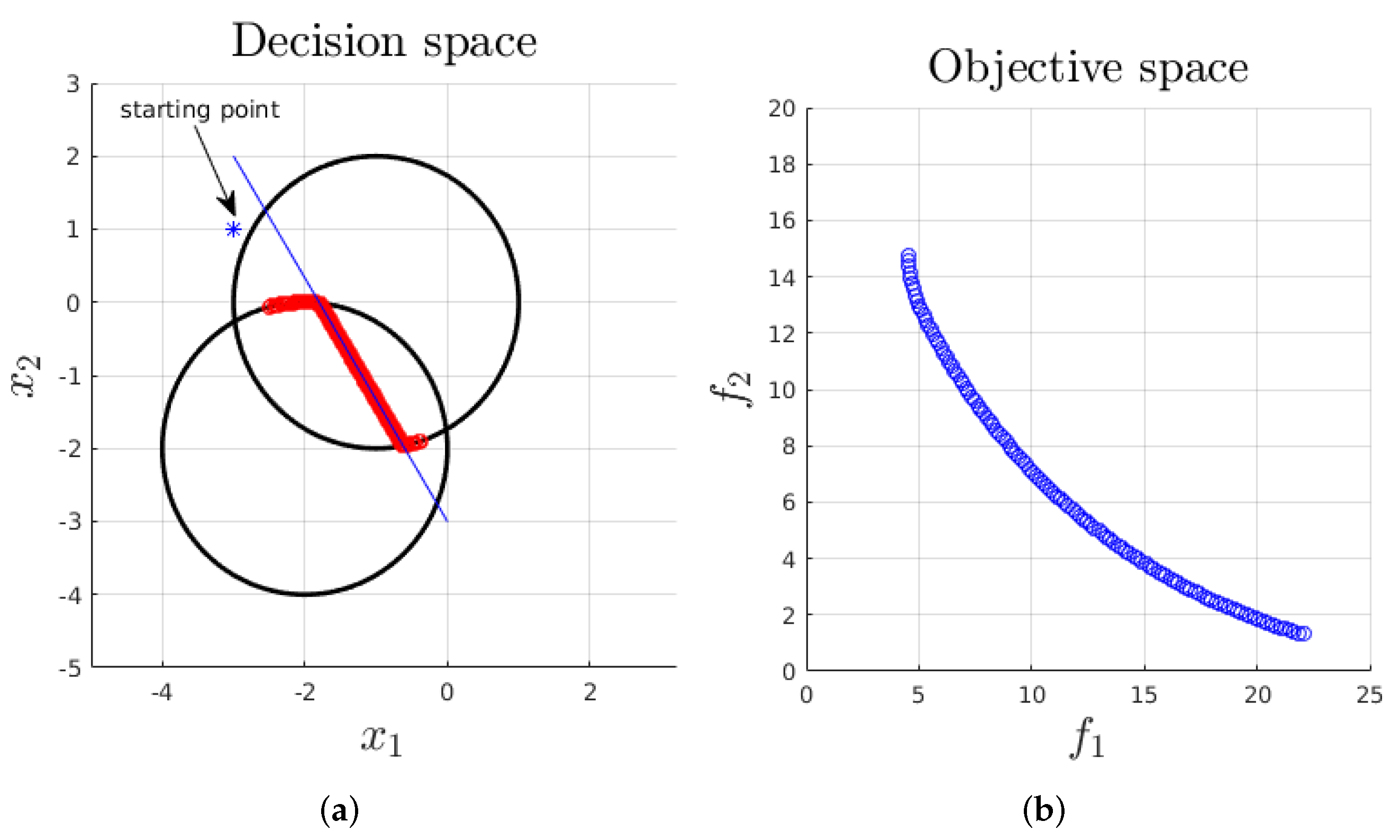
As a demonstration example, we consider the problem
Figure 1a shows the Pareto set of the above problem where the two inequalities have been left out (i.e., the line segment connecting and ), the sets , , as well as the Pareto set of this problem which is indeed the result of the PT. As starting point, we chose a point which significantly violates both constraints (and, hence, for ). An application of the above-described Newton method leads to the point on the Pareto set with the smallest -value, which is in fact the initial point for the PT. During the run of PT, first only is “active” in the corrector step (i.e., ), later none of the constraints (in the intersection of the Pareto fronts of the constrained and the unconstrained MOP), and finally only .
4. Numerical Results
In this section, we further demonstrate the behavior of the PT on five benchmark problems that contain inequality constraints. For all problems, we used the quasi-Newton variant of PT that only required function and Jacobian information (and no Hessians). To compare the results, we also show the respective results obtained by the normal boundary intersection (NBI, [16]), the -constraint method [5], and the multi-objective evolutionary algorithm NSGA-II. For NBI and the -constraint method, we used the code that is available at [52], and for NSGA-II the implementation of PlatEMO [53]. Regrettably, no comparison to a multi-objective continuation method can be presented since none of the respective codes are publicly available. For a comparison of the PT and the method of Hillermeier on box and equality constrained MOPs, we refer to [2]. We chose also to include a comparison to the famous NSGA-II since it is widely used and state-of-the-art for two- and three-objective problems as we consider here. We stress that the comparisons only show (on the first four test problems) that PT outperforms NSGA-II on these particular cases where the Pareto front consists of one connected component. For highly multi-modal functions where the Pareto set/front falls into several connected components, NSGA-II will certainly outperform the (standalone) PT. A fair comparison can only be obtained when integrating PT into a global heuristic (as, e.g., done in [41]). This is certainly an interesting task, however, beyond the scope of this work.
To compare the results, we compare the total number of function evaluations used for each algorithm on each problem. For this, each Jacobian call is counted as four function calls assuming that the derivative is obtained via automatic differentiation [54]. To measure the quality of the approximations, we used the averaged Hausdorff distance [55,56,57]. Since NSGA-II has stochastic components, we applied this algorithm for each problem 10 times and present the median result (measured by ).
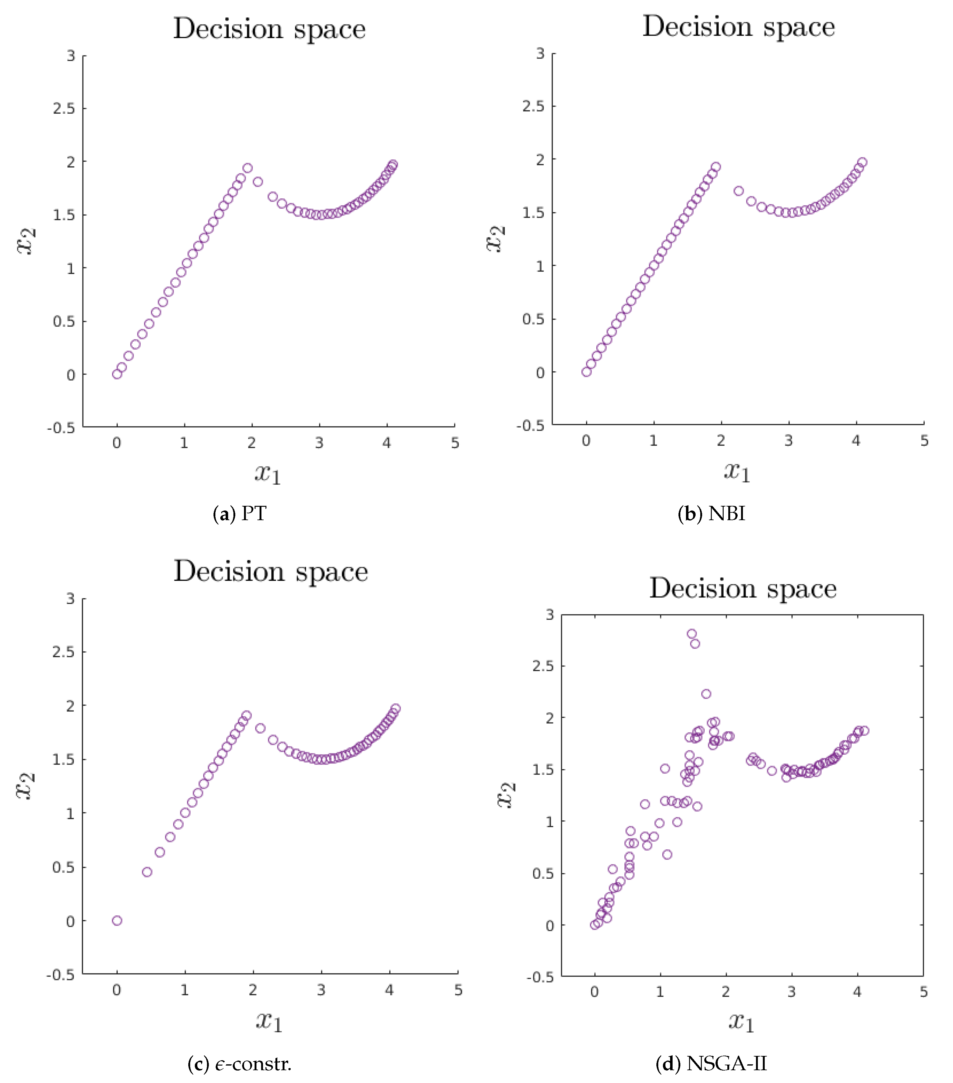
4.1. Binh and Korn
Our first test example is a modification of the box-constrained BOP from Binh and Korn [58], where we add two inequality constraints as follows:
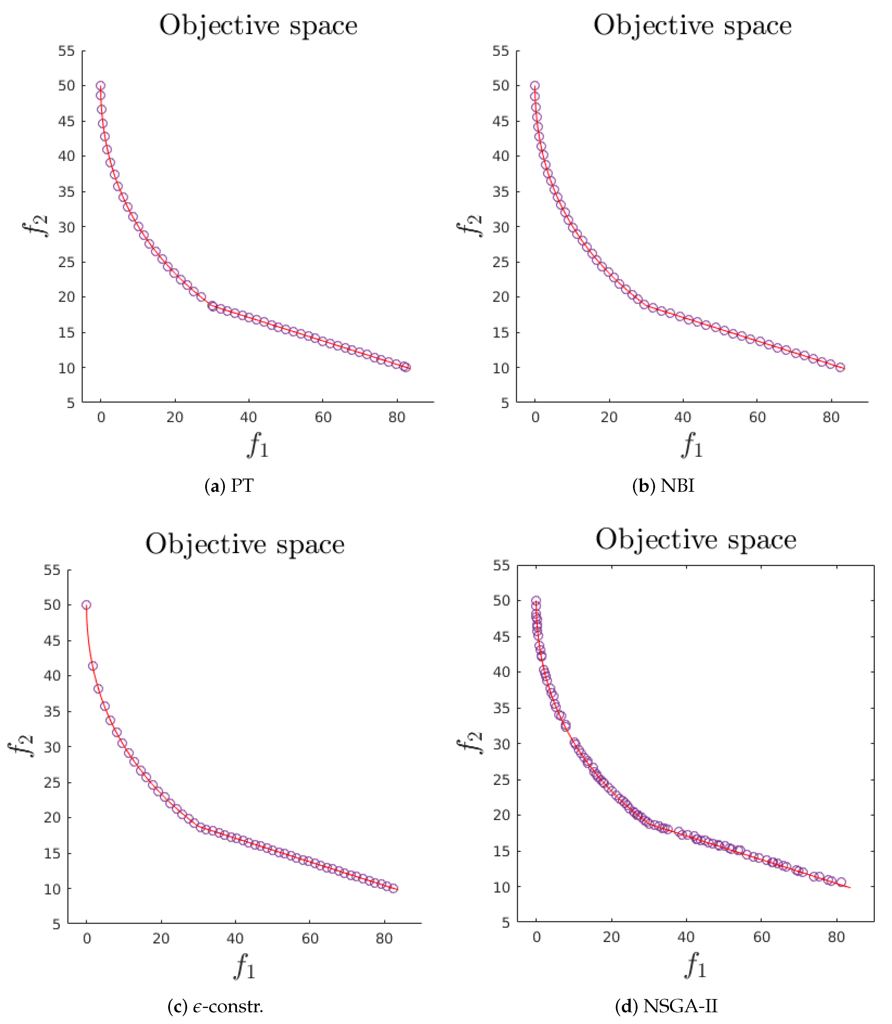
Table 1 shows the design parameters that have been used by NSGA-II for this problem, Table 2 shows the computational efforts and the obtained approximation quality for each algorithm, and Figure 2 and Figure 3 show the obtained Pareto set and front approximations, respectively. For PT, we chose leading to 52 solutions along the Pareto set/front in 4.48 s (the computations have been done on a Ubuntu 20.04.1 LTS system with an Intel Core i7-855OU 1.80 GHz x 8 CPU and 12 GB of RAM). We then applied NBI and the -constraint model using this number of sub-problems. For NSGA-II, we took the population size 100, which is a standard value for this algorithm. The results show nearly perfect Pareto front approximations (at least from the practical point of view) for all algorithms, which is also reflected by the low values that are very close to the optimal value of (at least for PT, defined by ). In terms of function evaluations, PT clearly wins over NBI and the -constraint method. A comparison to NSGA-II is not possible due to the choice of the population size.
4.2. Chakong and Haimes
Next, we consider the bi-objective problem of Chankong and Haimes [59], which contains next to the box constraints one linear and one nonlinear inequality.
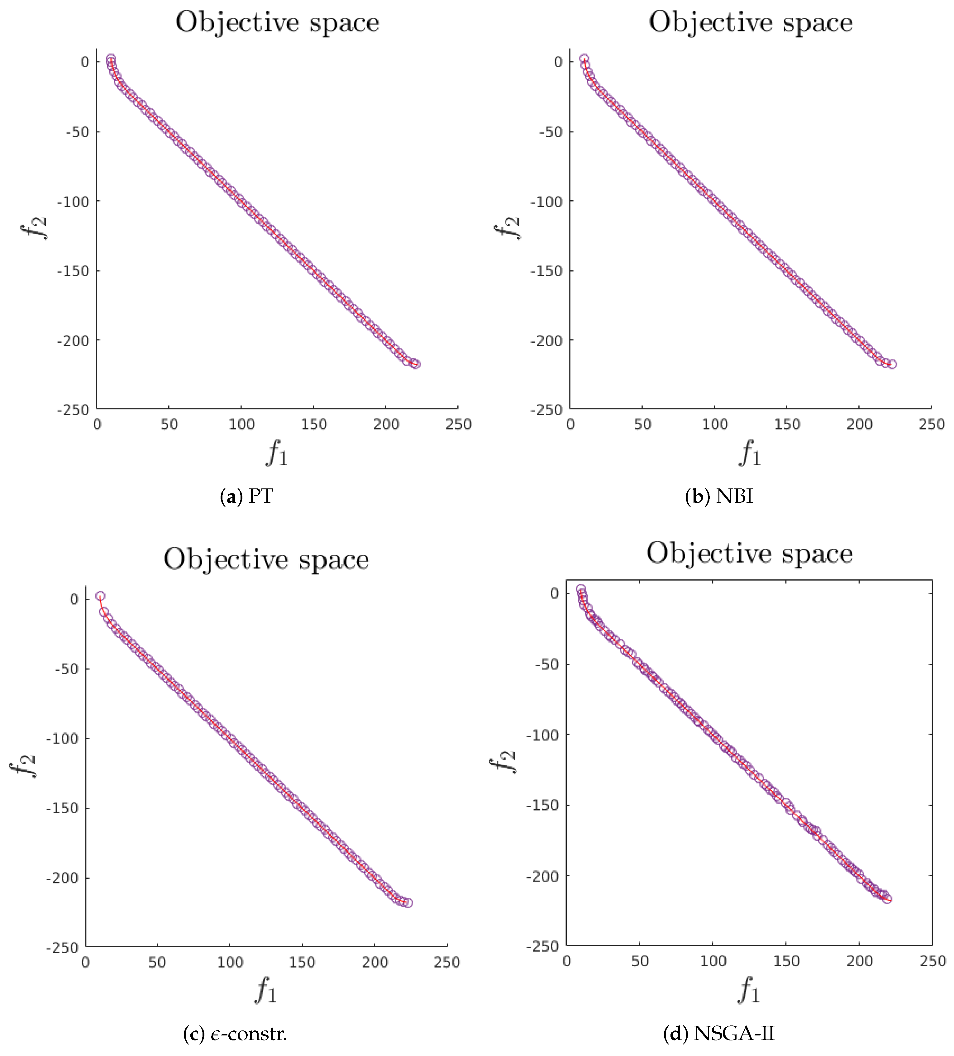
Table 3 shows the parameter values used for the application of NSGA-II, Table 4 the computational efforts and the approximation qualities, and Figure 4 and Figure 5 the obtained approximations. We used for PT, and proceeded as for the previous example for the other methods. The results are also similar to the previous example: all methods are capable of detecting a nearly perfect Pareto front approximation, and the overall cost is significantly less for PT, in 5.96 s.
4.3. Tamaki
Next, we considered a MOP with three objectives (28):
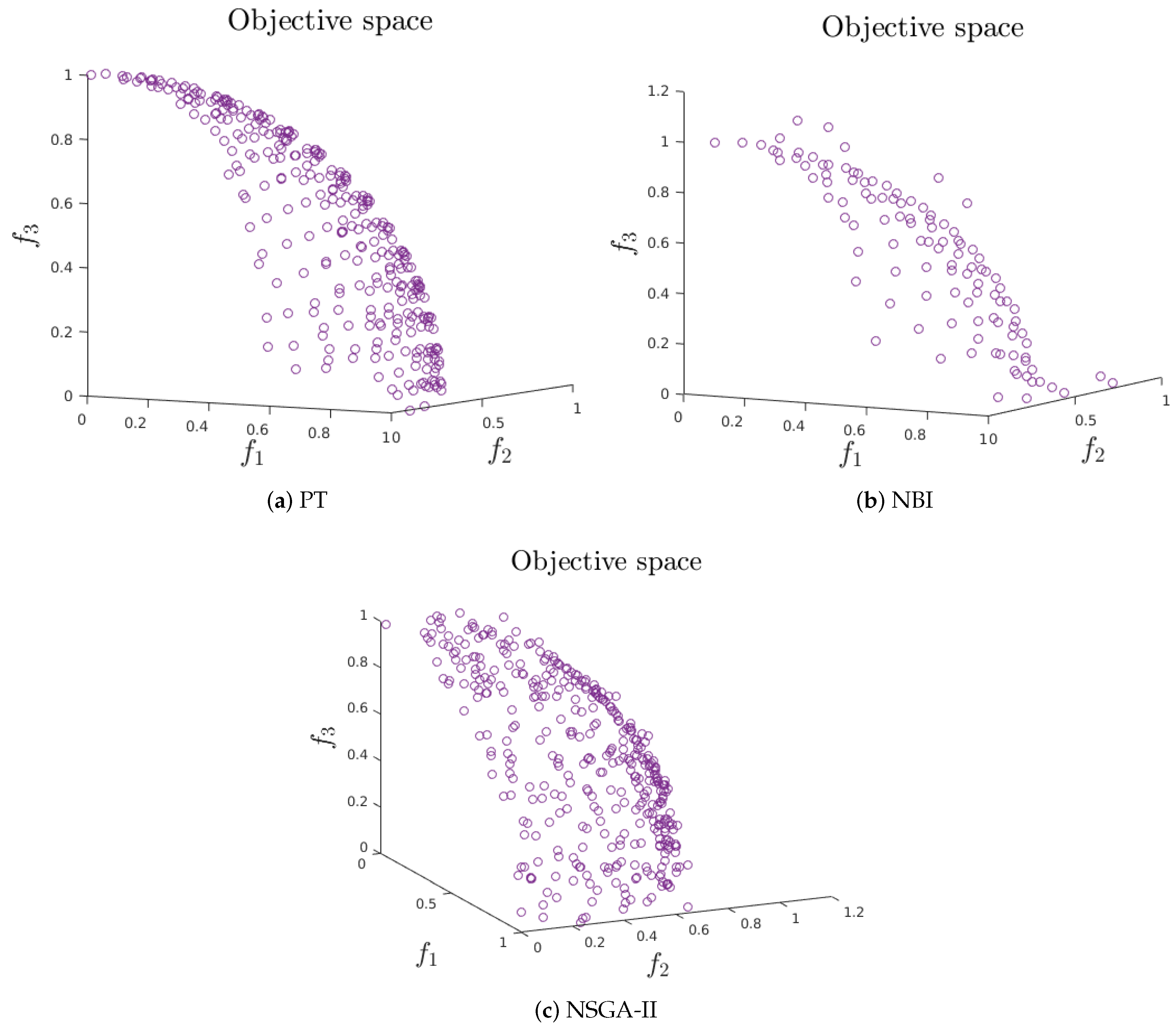
Both the Pareto set and front for this problem are a part of the unit sphere. Table 5 shows the design parameters for NSGA-II, Table 6 shows the computational effort and the approximation quality for each algorithm, and Figure 6 shows the Pareto front approximations (the respective Pareto set approximations will look identically, albeit in x-space). For this problem, was used. The implementation of the -constrained method did not yield a result. On the Tamaki problem, PT performs better than the other algorithms both in approximation quality and in the overall computational cost.
4.4. BCS
We next considered a second three-objective problem that contains next to one inequality also a linear equality constraint:
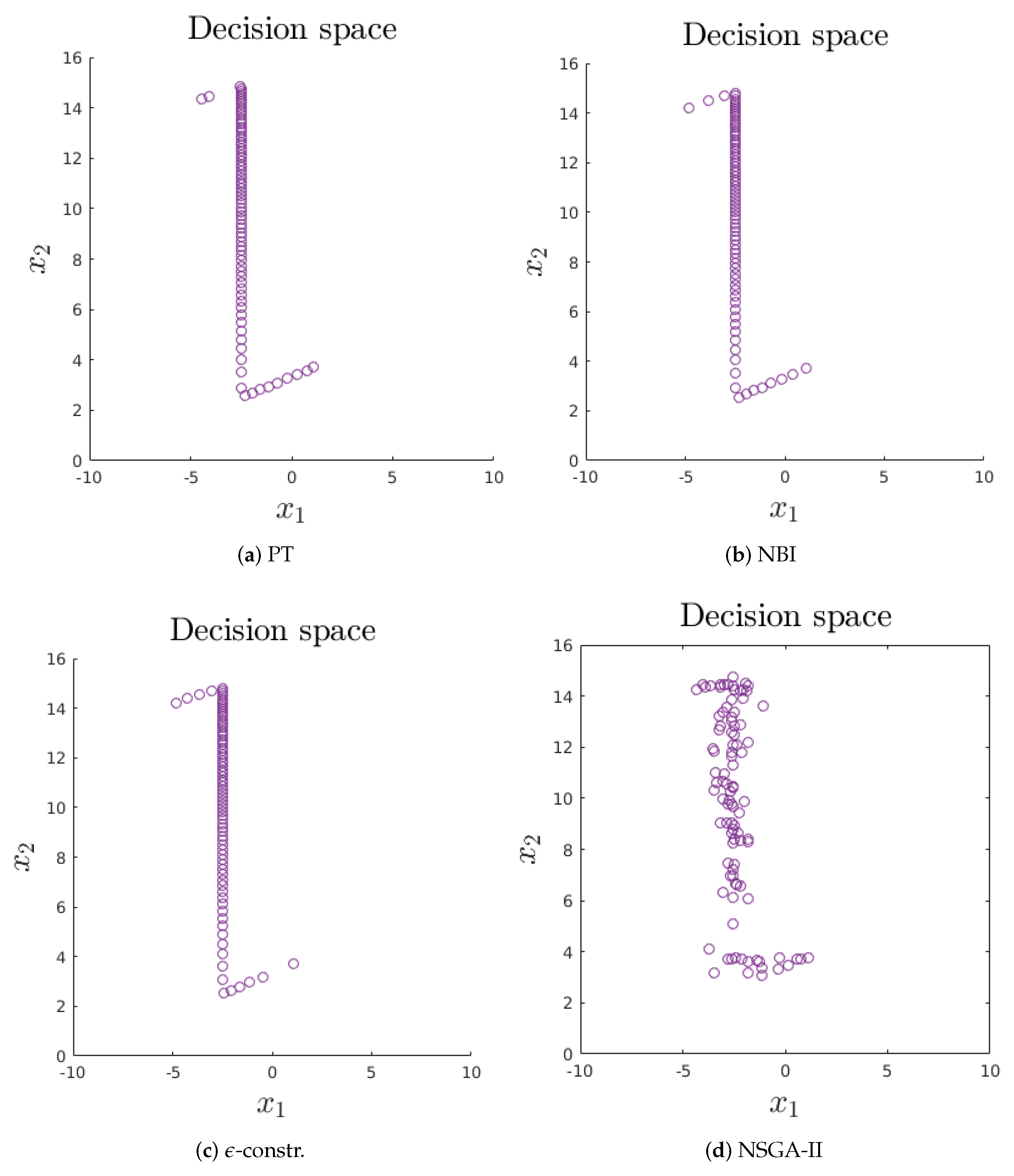
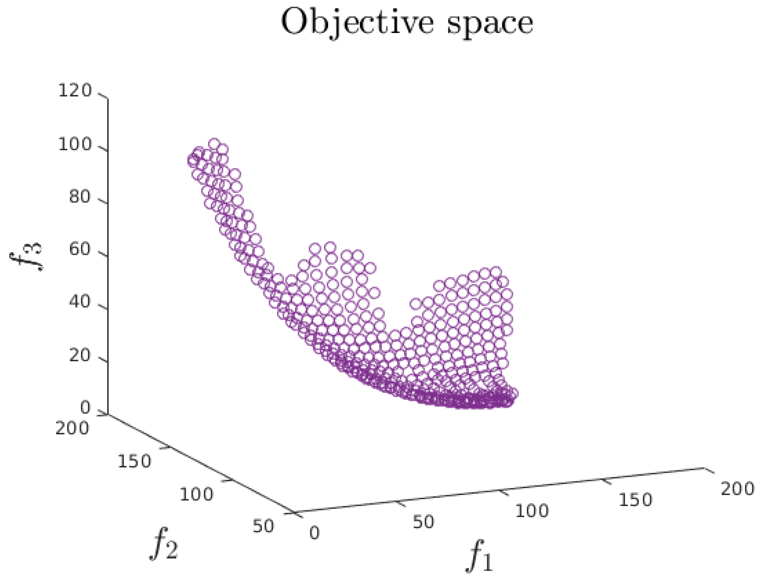
Table 7 presents the design parameters used by NSGA-II, Table 8 shows the computational effort and the approximation quality for each algorithm, and Figure 7 and Figure 8 present the Pareto front approximation of PT (using ), which took 16.79 s. For this example, none of the other methods were able to yield feasible solutions, where we counted a solution x to be feasible if and .
4.5. Osykzka and Kundu
As last example, we considered the bi-objective problem of Osykzka and Kundu [60], which has six decision variables and contains six inequality constraints in addition to the box constraints:
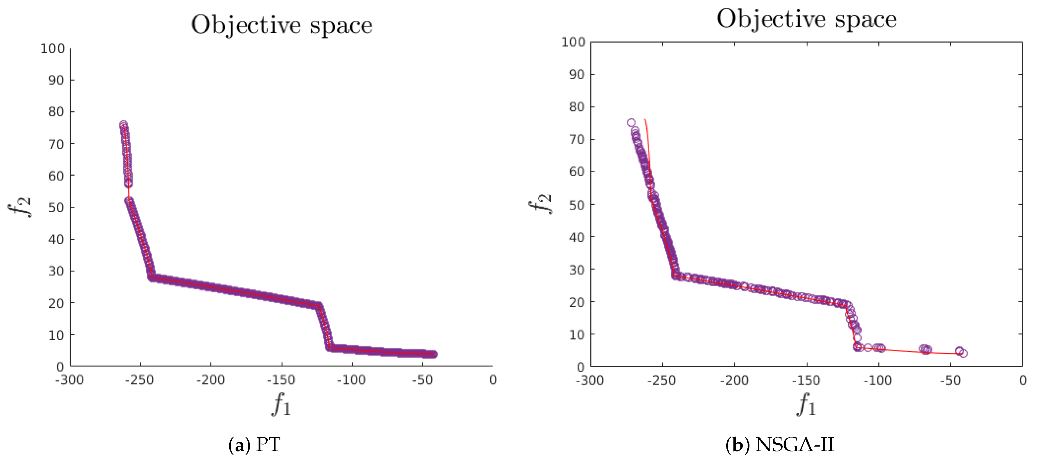
While the Pareto front of this problem is connected, its Pareto set consists of three different connected components. Hence, PT is not able to compute an approximation of the entire Pareto front with only one starting point. Figure 9a shows the result of PE for using the three starting points
The computational time to obtain this result was 12.98 s. Figure 9b shows a numerical result of NSGA-II using the design parameters shown in Table 9. The obtained solutions “under” the Pareto front can be explained by the tolerance of that was used to measure feasibility (while was used for PT). Table 10 shows the computational effort for both methods. Needless to say, this represents by no means a comparison of the two methods. Instead, this should be rather seen as a motivation to hybridize PT with a global search strategy in order to obtain a fast and reliable multi-objective solver, which we leave for future studies.
5. Conclusions and Future Work
In this paper, we extend the multi-objective continuation method Pareto Tracer (PT) for the treatment of general inequality constraints. To this end, the predictor–corrector step is modified as follows: in the predictor, all nearly active inequalities are treated as equalities. In the following corrector step, the main challenge is to identify the inequalities for which the predictor solution is either nearly active or slightly violates the constraint that has to be considered, namely the equality constraint in the Newton method, and this is done in a bootstrap manner. We formulate the resulting algorithm and show some numerical results on several benchmark problems, indicating that it can reliably handle inequality (and equality) constrained MOPs. We further present comparisons to some other numerical methods. The results show that the extended PT can indeed reliably handle general MOPs (and in particular general inequalities). However, the method is—by construction—of local nature and restricted to the connected component of the solution set for which one initial solution is available. One interesting task is certainly to hybridize PT with a global solver such as a multi-objective evolutionary algorithm and to compare the resulting hybrid against other methods with respect to their ability to compute the entire global Pareto set/front of a given MOP. This is beyond the scope of this work and has been left for future work.
Author Contributions
Conceptualization and formal analysis, O.S.; software, F.B. and O.C.; and writing and editing: F.B., O.C., and O.S. All authors have read and agreed to the published version of the manuscript.
Funding
The authors acknowledge support from Conacyt project No. 285599 and SEP Cinvestav project No. 231.
Conflicts of Interest
The authors declare no conflict of interest.
References
- Hillermeier, C. Nonlinear Multiobjective Optimization: A Generalized Homotopy Approach; Springer: Basel, Switzerland, 2001. [Google Scholar]
- Martín, A.; Schütze, O. Pareto Tracer: A predictor–corrector method for multi-objective optimization problems. Eng. Optim. 2018, 50, 516–536. [Google Scholar] [CrossRef]
- Deb, K. Multi-Objective Optimization Using Evolutionary Algorithms; John Wiley & Sons: Chichester, UK, 2001. [Google Scholar]
- Peitz, S.; Dellnitz, M. A Survey of Recent Trends in Multiobjective Optimal Control—Surrogate Models, Feedback Control and Objective Reduction. Math. Comput. Appl. 2018, 23, 30. [Google Scholar] [CrossRef] [Green Version]
- Miettinen, K. Nonlinear Multiobjective Optimization; Springer Science & Business Media: Boston, MA, USA, 2012. [Google Scholar]
- Ehrgott, M. Multicriteria Optimization; Springer: Berlin/Heidelberg, Germany, 2005. [Google Scholar]
- Karush, W. Minima of Functions of Several Variables with Inequalities as Side Constraints. Master’s Thesis, Department of Mathematics, University of Chicago, Chicago, IL, USA, 1939. [Google Scholar]
- Kuhn, H.W.; Tucker, A.W. Nonlinear programming. In Proceedings of the Second Berkeley Symposium on Mathematical Statistics and Probability, Berkeley, CA, USA, 31 July–12 August 1950; University of California Press: Berkeley, CA, USA, 1951; pp. 481–492. [Google Scholar]
- Gass, S.; Saaty, T. The computational algorithm for the parametric objective function. Nav. Res. Logist. Q. 1955, 2, 39–45. [Google Scholar] [CrossRef]
- Mavrotas, G. Effective implementation of the ϵ-constraint method in Multi-Objective Mathematical Programming problems. Appl. Math. Comput. 2009, 213, 455–465. [Google Scholar]
- Steuer, R.E.; Choo, E.U. An Interactive Weighted Tchebycheff Prodecure for Multiple Objective Progamming. Math. Program. 1983, 26, 326–344. [Google Scholar] [CrossRef]
- Kim, J.; Kim, S.K. A CHIM-based interactive Tchebycheff procedure for multiple objective decision making. Comput. Oper. Res. 2006, 33, 1557–1574. [Google Scholar] [CrossRef]
- Wierzbicki, A.P. A mathematical basis for satisficing decision making. Math. Model. 1982, 3, 391–405. [Google Scholar] [CrossRef] [Green Version]
- Bogetoft, P.; Hallefjord, A.; Kok, M. On the convergence of reference point methods in multiobjective programming. Eur. J. Oper. Res. 1988, 34, 56–68. [Google Scholar] [CrossRef]
- Hernández Mejá, J.A.; Schütze, O.; Cuate, O.; Lara, A.; Deb, K. RDS-NSGA-II: A Memetic Algorithm for Reference Point Based Multi-objective Optimization. Eng. Optim. 2017, 49, 828–845. [Google Scholar] [CrossRef]
- Das, I.; Dennis, J.E. Normal-boundary intersection: A new method for generating the Pareto surface in nonlinear multicriteria optimization problems. SIAM J. Optim. 1998, 8, 631–657. [Google Scholar] [CrossRef] [Green Version]
- Klamroth, K.; Tind, J.; Wiecek, M. Unbiased Approximation in Multicriteria Optimization. Math. Methods Oper. Res. 2002, 56, 413–437. [Google Scholar] [CrossRef]
- Fliege, J. Gap-free computation of Pareto-points by quadratic scalarizations. Math. Methods Oper. Res. 2004, 59, 69–89. [Google Scholar] [CrossRef]
- Eichfelder, G. Adaptive Scalarization Methods in Multiobjective Optimization; Springer: Berlin/Heidelberg, Germany, 2008. [Google Scholar]
- Hernández, C.; Naranjani, Y.; Sardahi, Y.; Liang, W.; Schütze, O.; Sun, J.Q. Simple Cell Mapping Method for Multi-objective Optimal Feedback Control Design. Int. J. Dyn. Control 2013, 1, 231–238. [Google Scholar] [CrossRef]
- Xiong, F.R.; Qin, Z.C.; Xue, Y.; Schütze, O.; Ding, Q.; Sun, J.Q. Multi-objective optimal design of feedback controls for dynamical systems with hybrid simple cell mapping algorithm. Commun. Nonlinear Sci. Numer. Simul. 2014, 19, 1465–1473. [Google Scholar] [CrossRef]
- Fernández, J.; Schütze, O.; Hernández, C.; Sun, J.Q.; Xiong, F.R. Parallel simple cell mapping for multi-objective optimization. Eng. Optim. 2016, 48, 1845–1868. [Google Scholar] [CrossRef]
- Sun, J.Q.; Xiong, F.R.; Schütze, O.; Hernández, C. Cell Mapping Methods—Algorithmic Approaches and Applications; Springer: Singapore, 2019. [Google Scholar]
- Schütze, O.; Mostaghim, S.; Dellnitz, M.; Teich, J. Covering Pareto Sets by Multilevel Evolutionary Subdivision Techniques. In Proceedings of the International Conference on Evolutionary Multi-Criterion Optimization (EMO 2003), Faro, Portugal, 8–11 April 2003; Fonseca, C.M., Fleming, P.J., Zitzler, E., Deb, K., Thiele, L., Eds.; Springer: Berlin/Heidelberg, Germany, 2003; pp. 118–132. [Google Scholar]
- Dellnitz, M.; Schütze, O.; Hestermeyer, T. Covering Pareto Sets by Multilevel Subdivision Techniques. J. Optim. Theory Appl. 2005, 124, 113–155. [Google Scholar] [CrossRef]
- Jahn, J. Multiobjective search algorithm with subdivision technique. Comput. Optim. Appl. 2006, 35, 161–175. [Google Scholar] [CrossRef]
- Schütze, O.; Vasile, M.; Junge, O.; Dellnitz, M.; Izzo, D. Designing optimal low thrust gravity assist trajectories using space pruning and a multi-objective approach. Eng. Optim. 2009, 41, 155–181. [Google Scholar] [CrossRef] [Green Version]
- Deb, K.; Pratap, A.; Agarwal, S.; Meyarivan, T. A fast and elitist multiobjective genetic algorithm: NSGA-II. IEEE Trans. Evol. Comput. 2002, 6, 182–197. [Google Scholar] [CrossRef] [Green Version]
- Coello Coello, C.A.; Lamont, G.B.; Van Veldhuizen, D.A. Evolutionary Algorithms for Solving Multi-Objective Problems, 2nd ed.; Springer: New York, NY, USA, 2007. [Google Scholar]
- Beume, N.; Naujoks, B.; Emmerich, M. SMS-EMOA: Multiobjective selection based on dominated hypervolume. Eur. J. Oper. Res. 2007, 181, 1653–1669. [Google Scholar] [CrossRef]
- Lara, A.; Sanchez, G.; Coello Coello, C.A.; Schütze, O. HCS: A new local search strategy for memetic multiobjective evolutionary algorithms. IEEE Trans. Evol. Comput. 2009, 14, 112–132. [Google Scholar] [CrossRef]
- Zhou, A.; Qu, B.Y.; Li, H.; Zhao, S.Z.; Suganthan, P.N.; Zhang, Q. Multiobjective evolutionary algorithms: A survey of the state of the art. Swarm Evol. Comput. 2011, 1, 32–49. [Google Scholar] [CrossRef]
- Cuate, O.; Schütze, O. Variation Rate to Maintain Diversity in Decision Space within Multi-Objective Evolutionary Algorithms. Math. Comput. Appl. 2019, 24, 82. [Google Scholar] [CrossRef] [Green Version]
- Schütze, O.; Hernández, C. Archiving Strategies for Evolutionary Multi-objective Optimization Algorithms; Springer: Cham, Switzerland, 2021. [Google Scholar]
- Harada, K.; Sakuma, J.; Kobayashi, S. Local search for multiobjective function optimization: Pareto descent method. In Proceedings of the 8th Annual Conference on Genetic and Evolutionary Computation, Seattle, WA, USA, 8–12 July 2006; pp. 659–666. [Google Scholar]
- Schütze, O.; Coello, C.A.C.; Mostaghim, S.; Dellnitz, M.; Talbi, E.G. Hybridizing Evolutionary Strategies with Continuation Methods for Solving Multi-objective Problems. IEEE Trans. Evol. Comput. 2008, 19, 762–769. [Google Scholar] [CrossRef]
- Zapotecas Martínez, S.; Coello Coello, C.A. A proposal to hybridize multi-objective evolutionary algorithms with non-gradient mathematical programming techniques. In Proceedings of the 10th International Conference on Parallel Problem Solving From Nature (PPSN ’08), Dortmund, Germany, 13–17 September 2008; pp. 837–846. [Google Scholar]
- Bosman, P.A.N. On gradients and hybrid evolutionary algorithms for real-valued multiobjective optimization. IEEE Trans. Evol. Comput. 2011, 16, 51–69. [Google Scholar] [CrossRef]
- Schütze, O.; Martín, A.; Lara, A.; Alvarado, S.; Salinas, E.; Coello, C.A. The Directed Search Method for Multiobjective Memetic Algorithms. J. Comput. Optim. Appl. 2016, 63, 305–332. [Google Scholar] [CrossRef]
- Schütze, O.; Alvarado, S.; Segura, C.; Landa, R. Gradient subspace approximation: A direct search method for memetic computing. Soft Comput. 2016, 21, 6331–6350. [Google Scholar] [CrossRef]
- Cuate, O.; Ponsich, A.; Uribe, L.; Zapotecas, S.; Lara, A.; Schütze, O. A New Hybrid Evolutionary Algorithm for the Treatment of Equality Constrained MOPs. Mathematics 2020, 8, 7. [Google Scholar] [CrossRef] [Green Version]
- Martin, B.; Goldsztejn, A.; Granvilliers, L.; Jermann, C. Certified Parallelotope Continuation for One-Manifolds. SIAM J. Numer. Anal. 2013, 51, 3373–3401. [Google Scholar] [CrossRef]
- Martin, B.; Goldsztejn, A.; Granvilliers, L.; Jermann, C. On continuation methods for non-linear bi-objective optimization: Towards a certified interval-based approach. J. Glob. Optim. 2014, 64, 3–16. [Google Scholar] [CrossRef] [Green Version]
- Pereyra, V.; Saunders, M.; Castillo, J. Equispaced Pareto front construction for constrained bi-objective optimization. Math. Comput. Model. 2013, 57, 2122–2131. [Google Scholar] [CrossRef]
- Wang, H. Zigzag Search for Continuous Multiobjective Optimization. Inf. J. Comput. 2013, 25, 654–665. [Google Scholar] [CrossRef]
- Wang, H. Direct zigzag search for discrete multi-objective optimization. Comput. Oper. Res. 2015, 61, 100–109. [Google Scholar] [CrossRef]
- Zhang, Q.; Li, F.; Wang, H.; Xue, Y. Zigzag search for multi-objective optimization considering generation cost and emission. Appl. Energy 2019, 255. [Google Scholar] [CrossRef]
- Recchioni, M.C. A path following method for box-constrained multiobjective optimization with applications to goal programming problems. Math. Methods Oper. Res. 2003, 58, 69–85. [Google Scholar] [CrossRef]
- Ringkamp, M.; Ober-Blöbaum, S.; Dellnitz, M.; Schütze, O. Handling high dimensional problems with multi-objective continuation methods via successive approximation of the tangent space. Eng. Optim. 2012, 44, 1117–1146. [Google Scholar] [CrossRef]
- Schütze, O.; Cuate, O.; Martín, A.; Peitz, S.; Dellnitz, M. Pareto Explorer: A global/local exploration tool for many-objective optimization problems. Eng. Optim. 2020, 52, 832–855. [Google Scholar] [CrossRef]
- Fliege, J.; Drummond, L.M.G.; Svaiter, B.F. Newton’s Method for Multiobjective Optimization. SIAM J. Optim. 2009, 20, 602–626. [Google Scholar] [CrossRef] [Green Version]
- Julia. JuMP—Julia for Mathematical Optimization. Available online: http://www.juliaopt.org/JuMP.jl/v0.14/ (accessed on 17 December 2020).
- Tian, Y.; Cheng, R.; Zhang, X.; Jin, Y. PlatEMO: A MATLAB platform for evolutionary multi-objective optimization [educational forum]. IEEE Comput. Intell. Mag. 2017, 12, 73–87. [Google Scholar] [CrossRef] [Green Version]
- Griewank, A.; Walther, A. Evaluating Derivatives: Principles and Techniques of Algorithmic Differentiation; SIAM: Philadelphia, PA, USA, 2008. [Google Scholar]
- Schütze, O.; Esquivel, X.; Lara, A.; Coello, C.A.C. Using the Averaged Hausdorff Distance as a Performance Measure in Evolutionary Multi-Objective Optimization. IEEE Trans. Evol. Comput. 2012, 16, 504–522. [Google Scholar] [CrossRef]
- Bogoya, J.M.; Vargas, A.; Cuate, O.; Schütze, O. A (p, q)-averaged Hausdorff distance for arbitrary measurable sets. Math. Comput. Appl. 2018, 23, 51. [Google Scholar] [CrossRef] [Green Version]
- Bogoya, J.M.; Vargas, A.; Schütze, O. The Averaged Hausdorff Distances in Multi-Objective Optimization: A Review. Mathematics 2019, 7, 894. [Google Scholar] [CrossRef] [Green Version]
- Binh, T.T.; Korn, U. MOBES: A multiobjective evolution strategy for constrained optimization problems. In Proceedings of the Third International Conference on Genetic Algorithms (Mendel 97), Brno, Czech Republic, 25–27 June 1997; Volume 25, pp. 176–182. [Google Scholar]
- Chankong, V.; Haimes, Y. Multiobjective Decision Making: Theory and Methodology; Dover Publications: Mineola, NY, USA, 2008. [Google Scholar]
- Osyczka, A.; Kundu, S. A new method to solve generalized multicriteria optimization problems using the simple genetic algorithm. Struct. Optim. 1995, 10, 94–99. [Google Scholar] [CrossRef]
Figure 1.
Numerical result of the PT for MOP (25).
Figure 1.
Numerical result of the PT for MOP (25).

Figure 2.
Results in decision space for MOP (26).
Figure 2.
Results in decision space for MOP (26).

Figure 3.
Results in objective space for MOP (26).
Figure 3.
Results in objective space for MOP (26).

Figure 4.
Results in decision space for MOP (27).
Figure 4.
Results in decision space for MOP (27).

Figure 5.
Results in objective space for MOP (27).
Figure 5.
Results in objective space for MOP (27).

Figure 6.
Results in objective space for MOP (28).
Figure 6.
Results in objective space for MOP (28).

Figure 7.
Numerical result of PT in the decision space for MOP (29).
Figure 7.
Numerical result of PT in the decision space for MOP (29).

Figure 8.
Numerical result of PT in the objective space for MOP (29).
Figure 8.
Numerical result of PT in the objective space for MOP (29).

Figure 9.
Results in objective space for MOP (30).
Figure 9.
Results in objective space for MOP (30).


Table 1.
Parameters used by NSGA-II for MOP (26).
Table 1.
Parameters used by NSGA-II for MOP (26).
| Population Size | 100 |
| Number of generations | 20 |
| Probability of crossover | 0.9 |
| Probability of mutation | 0.5 |
Table 2.
Computational efforts and approximation quality of the algorithms for MOP (26).
Table 2.
Computational efforts and approximation quality of the algorithms for MOP (26).
| PT | NBI | -Constr. | NSGA-II | |
|---|---|---|---|---|
| Solutions | 52 | 52 | 52 | 100 |
| Function Evaluations | 151 | 427 | 336 | 2000 |
| Jacobian Evaluations | 133 | 425 | 336 | - |
| Hessian Evaluations | - | 373 | 284 | - |
| Total of Evaluations | 683 | 8095 | 6224 | 2000 |
| 0.6050 | 0.6025 | 0.9272 | 0.5626 |
Table 3.
Parameters used by NSGA-II for problem (27).
Table 3.
Parameters used by NSGA-II for problem (27).
| Population Size | 100 |
| Number of generations | 30 |
| Probability of crossover | 0.9 |
| probability of mutation | 0.5 |
Table 4.
Computational efforts and approximation qualities for problem (27).
Table 4.
Computational efforts and approximation qualities for problem (27).
| PT | NBI | -Constr. | NSGA-II | |
|---|---|---|---|---|
| Solutions | 80 | 80 | 80 | 100 |
| Function Evaluations | 540 | 678 | 578 | 3000 |
| Jacobian Evaluations | 499 | 678 | 578 | - |
| Hessian Evaluations | - | 598 | 498 | - |
| Total of Evaluations | 2536 | 12,958 | 10,858 | 3000 |
| 1.1459 | 1.1457 | 1.2141 | 1.1871 |
Table 5.
Parameters used by NSGA-II for MOP (28).
Table 5.
Parameters used by NSGA-II for MOP (28).
| Population Size | 300 |
| Number of generations | 150 |
| Probability of crossover | 0.9 |
| Probability of mutations | 0.5 |
Table 6.
Computational efforts and approximation qualities for problem (28).
Table 6.
Computational efforts and approximation qualities for problem (28).
| PT | NBI | -Constr. | NSGA-II | |
|---|---|---|---|---|
| Solutions | 305 | 112 | N/A | 300 |
| Function Evaluations | 2498 | 3758 | N/A | 450,000 |
| Jacobian Evaluations | 1101 | 3758 | N/A | - |
| Hessian Evaluations | - | 3293 | N/A | - |
| Total of Evaluations | 6902 | 91,236 | N/A | 450,000 |
| 0.0380 | 0.6353 | N/A | 0.0390 |
Table 7.
Parameters used by NSGA-II for MOP (29).
Table 7.
Parameters used by NSGA-II for MOP (29).
| Population Size | 100 |
| Number of generations | 500 |
| Probability of crossover | 0.9 |
| Probability of mutations | 0.5 |
Table 8.
Computation efforts for the proposed test problem (29).
Table 8.
Computation efforts for the proposed test problem (29).
| PT | NBI | -Constr. | NSGA-II | |
|---|---|---|---|---|
| Solutions | 378 | 0 | N/A | 4 |
| Function Evaluations | 1923 | 2290 | N/A | 50,000 |
| Jacobian Evaluations | 756 | 1641 | N/A | - |
| Hessian Evaluations | - | 1431 | N/A | - |
| Total of Evaluations | 4947 | 40,336 | N/A | 50,000 |
| 2.0658 | - | N/A | 61.7685 |
Table 9.
Parameters used by NSGA-II for MOP (30).
Table 9.
Parameters used by NSGA-II for MOP (30).
| Population Size | 435 |
| Number of generations | 50 |
| Probability of crossover | 0.9 |
| Probability of mutations | 0.5 |
Table 10.
Computational efforts and approximation qualities for problem (30).
Table 10.
Computational efforts and approximation qualities for problem (30).
| PT | NSGA-II | |
|---|---|---|
| Solutions | 435 | 428 |
| Function Evaluations | 2051 | 20,000 |
| Jacobian Evaluations | 850 | - |
| Hessian Evaluations | - | - |
| Total of Evaluations | 5451 | 20,000 |
| 1.801 | 2.4819 |
Publisher’s Note: MDPI stays neutral with regard to jurisdictional claims in published maps and institutional affiliations. |
© 2020 by the authors. Licensee MDPI, Basel, Switzerland. This article is an open access article distributed under the terms and conditions of the Creative Commons Attribution (CC BY) license (http://creativecommons.org/licenses/by/4.0/).
Share and Cite
MDPI and ACS Style
Beltrán, F.; Cuate, O.; Schütze, O. The Pareto Tracer for General Inequality Constrained Multi-Objective Optimization Problems. Math. Comput. Appl. 2020, 25, 80. https://0-doi-org.brum.beds.ac.uk/10.3390/mca25040080
AMA Style
Beltrán F, Cuate O, Schütze O. The Pareto Tracer for General Inequality Constrained Multi-Objective Optimization Problems. Mathematical and Computational Applications. 2020; 25(4):80. https://0-doi-org.brum.beds.ac.uk/10.3390/mca25040080
Chicago/Turabian StyleBeltrán, Fernanda, Oliver Cuate, and Oliver Schütze. 2020. "The Pareto Tracer for General Inequality Constrained Multi-Objective Optimization Problems" Mathematical and Computational Applications 25, no. 4: 80. https://0-doi-org.brum.beds.ac.uk/10.3390/mca25040080