A Framework for Analysis and Prediction of Operational Risk Stress


Department of Computer Science, University College London, Gower Street, London WC1E 6BT, UK
Math. Comput. Appl. 2021, 26(1), 19; https://0-doi-org.brum.beds.ac.uk/10.3390/mca26010019
Submission received: 6 January 2021
/
Revised: 16 February 2021
/
Accepted: 19 February 2021
/
Published: 24 February 2021
(This article belongs to the Special Issue Numerical and Symbolic Computation: Developments and Applications 2021)
Abstract
:A model for financial stress testing and stability analysis is presented. Given operational risk loss data within a time window, short-term projections are made using Loess fits to sequences of lognormal parameters. The projections can be scaled by a sequence of risk factors, derived from economic data in response to international regulatory requirements. Historic and projected loss data are combined using a lengthy nonlinear algorithm to calculate a capital reserve for the upcoming year. The model is embedded in a general framework, in which arrays of risk factors can be swapped in and out to assess their effect on the projected losses. Risk factor scaling is varied to assess the resilience and stability of financial institutions to economic shock. Symbolic analysis of projected losses shows that they are well-conditioned with respect to risk factors. Specific reference is made to the effect of the 2020 COVID-19 pandemic. For a 1-year projection, the framework indicates a requirement for an increase in regulatory capital of approximately 3% for mild stress, 8% for moderate stress, and 32% for extreme stress. The proposed framework is significant because it is the first formal methodology to link financial risk with economic factors in an objective way without recourse to correlations.
Keywords:
risk factor; stress testing; economic stress; Loess; lognormal; regulatory capital; COVID-19; R; Mathematica1. Introduction
Every year, financial institutions (banks, insurance companies, financial advisors, etc.) have to demonstrate that they are resilient to adverse economic conditions. To do that, they are required to calculate what level of capital reserves would be necessary for the upcoming year. The requirements are specified in central bank publications such as from the Bank of England (BoE) [1], the European Central Bank (ECB) [2], or the Federal Reserve Bank (Fed) [3]. The following quote is taken from the introduction in the BoE’s stress test guidance [1]:
“The main purpose of the stress-testing framework is to provide a forward-looking, quantitative assessment of the capital adequacy of the UK banking system as a whole, and individual institutions within it.”
The particular terms forward-looking and quantitative are important for the analysis presented in this paper. Our stress framework incorporates both of those requirements.
The regulations concentrate on what financial instruments should be included and on the operational principles involved (data security, data collections, time deadlines, etc.). They say nothing about how stress testing should be conducted. The purpose of this paper is to provide a general-purpose framework that details not only how stress testing can be done but also a mathematical basis and practical steps for stress testing. The methodology presented is based on a principle that, under conditions of economic stress, there is a need to retain sufficient capital to withstand potential shocks to the banking system, whether or not any direct causal relationship exists between economic conditions and financial performance. Retaining capital is therefore effectively an insurance.
1.1. Operational Risk: A Brief Overview
The context considered in this paper is operational risk, which arises from adverse events that result in monetary loss. Operational risk may be summarised in the following definition from the Bank for International Settlements [4]:
“The risk of loss resulting from inadequate or failed internal processes, people and systems or from external events”
Each operational risk loss is a charge against the profit on a balance sheet and is fixed in time (although subsequent error corrections do occur). Operational risk falls in the category of non-financial risk and is therefore distinct form the principal components of financial risk: market, credit, and liquidity. The essential distinction is that financial risk arises from investment and trading, whereas non-financial risk arises from anything else (reputation, regulatory environment, legal events, conduct, physical events, decision-making, etc.). A useful categorisation of events that results in operational risk may be found at https://www.wallstreetmojo.com/operational-risks/ (accessed on 6 January 2021): human and technical error, fraud, uncontrollable events (such as physical damage and power outages), and process flow (procedural errors). The only way to manage operational risk is by preventing adverse events from occurring (e.g., acting within the law) or by minimising the effects if they do occur (e.g., mitigating the amount of fraud). When losses do occur, their values range from a few pounds (or dollars or euros) to multi-millions.
The following list shows illustrations of the comments above.
- The data used for this study (Section 4.1) did not include costs specific to the COVID-19 pandemic. Subsequently, £10 m was allocated to the costs of erecting protective perspex screens in UK bank branches.
- Repair costs following arson at the Wells Fargo Bank in Visalia, California, were estimated at $100,000. See https://eu.visaliatimesdelta.com/story/news/2020/04/22/arsonist-sets-fire-wells-fargo-causing-100-k-damage/3005549001/ (accessed on 6 January 2021).
- In October 2020, Goldman Sachs was fined £48,308,400 for breaches of conduct regulations (https://www.fca.org.uk/news/news-stories/2020-fines (accessed on 6 January 2021)).
- Monzo Bank reimbursed a customer £19,000 following an authorised push payment fraud (https://www.lovemoney.com/news/97578/authorised-push-payment-scam-compromised-account-direct-debits (accessed on 6 January 2021)).
- Smaller items included in the data set used for this study (see Section 4.1) include £9 (“compensation payment”), £10 (“reconciliation write-off”), and £68 (marked as “Simply thank you”).
1.2. Acronyms and Abbreviations
The following acronyms and abbreviations are used in this paper. Most are in common usage in the field of operational risk.
- OpRisk: Operational Risk
- VaR: Value-at-Risk
- CPBP: Clients, Products, and Business Practices, one of the seven categories discussed Section 1.3
- IF, EF, EPWS, DPA, BDSF, and EDPM: The remaining six risk categories. They are defined in Section 1.3
- Capital: Cash retained by banks annually for use as a buffer against unforeseen expenditure, details of which are specified by national regulatory bodies
- CCAR: Comprehensive Capital Analysis and Review (the US stress test regulations)
- FSF: Forward Stress Framework (the methodology presented in this paper)
- BoE: Bank of England
- ECB: European Central Bank
- Fed: Federal Reserve Bank
- GoF: Goodness-of-Fit (in the context of statistical distributions)
- TNA: The Transformed Normal ’A’ goodness-of-fit test, discussed in reference [5].
Less used acronyms and abbreviations are introduced within the main text. The categorisations introduced in Section 1.3 are only used incidentally.
1.3. Operational Risk: Categorisation
OpRisk capital is usually calculated in terms of value-at-risk (VaR [6]). VaR is defined as the maximum monetary amount expected to be lost over a given time horizon at a pre-defined confidence level. The 99.9% confidence level is specified worldwide as the standard benchmark for evaluating financial risk. VaR at 99.9% is often referred to as regulatory capital.
In this paper, the term capital is used to mean “value-at-risk of historic OpRisk losses at 99.9%” and a 3-month (i.e., -year) time horizon is referred to as a “quarter”.
OpRisk losses are classified worldwide into 7 categories, as specified originally in a data collection exercise from the Bank of International Settlements (the “Basel Committee”) [7]. The categories are Internal Fraud (IF); External Fraud (EF); Employment Practices and Workplace Safety (EPWS); Clients, Products, and Business Practices (CPBP); Damage to Physical Assets (DPA); Business Disruption and System Failures (BDSF); and Execution, Delivery, and Process Management (EDPM). Of these, CPBP is often treated in a different way from the others because it tends to contain exceptionally large losses, which distort calculated capital values unacceptable. See, for example, [8] or [9]. Consequently, that category is excluded from this analysis. Losses in the others are aggregated to provide sufficiently large samples. In this paper, that aggregation is referred to as risk category nonCPBP.
1.4. Operational Risk: Measurement
The most common procedure for measuring VaR is a Monte Carlo method known as the Loss Distribution Approach (LDA) [10]. After fitting a (usually fat-tailed) distribution to data, there are three steps in the LDA, which is a convolution of frequency and severity distributions. First, a single draw is made from a Poisson distribution with a parameter equal to the mean annual loss frequency. That determines the number of draws, N, for the next step. In step 2, N draws are taken from the fitted severity distribution. The sum of those draws represents a potential total loss for the upcoming year. Step 2 is repeated multiple times (typically 1 million), giving a population of total annual losses, L. In step 3, for a P% confidence level, the minimum loss that is larger than the Pth percentile of L is identified and is designated “P% VaR”. The LDA process is applicable for any severity distribution, which is why it is in common use. However, each complete Monte Carlo analysis can take up to 10 minutes to complete if sampling is slow and if the sample size is large.
2. Literature Review
We first summarise general approaches to stress testing and then review correlation relationships, since they are relevant for the Fed’s stress testing methodology.
2.1. Stress Testing Regulatory History
The early history of stress testing is traced in a general publication from the Financial Stability Institute (part of the Bank for International Settlements) [11]. Stress testing appeared in the early 1990s and was mainly developed by individual banks for internal risk management and to evaluate a bank’s trading activities [12]. A more coherent approach in the context of trading portfolios started with the 1996 “Basel Committee” regulations [13]. Regulation increased markedly following the 2008 financial crisis, mainly aimed at specifying what institutions and products should be regulated. The 2018 Bank for International Settlements publication [14] reiterated the aims and objectives of stress testing but without specific details on how tests should be conducted.
2.2. Financial Stress Testing Approaches
Regulatory guidance in the UK and EU documents [1] and [2] is circulated to financial institutions with historic and projected economic data on, among others, GDP, residential property prices, commercial real estate prices, the unemployment rate, foreign exchange rates, and interest rates. The data are intended to be used in conjunction with financial data, but no guidance is given as to how. There is no widely accepted categorisation for stress testing methods. Axtria Inc. [15] partitions approaches into “Parameter Stressing” and “Risk Driver Stressing”. Our approach corresponds to a mixture of the two. Otherwise, approaches may be classified by their mathematical or statistical approach.
2.2.1. Forward Stress Testing
The basis of “Forward” Stress testing is set out explicitly by Drehmann [16]. The process comprises four stages: scenario generation, developing risk factors, calculating exposures, and measuring the resulting risk. Stages 2 and 3 of that sequence may be summarised by Equation (1), in which represents an algorithm that calculates , the capital at time t. The arguments of are two vectors, both at time t: losses and stress factors . The precise way in which they are used remains to be defined precisely.
2.2.2. Reverse Stress Testing
In reverse stress testing [17], a desired level of stress in the target metric is decided in advance and the necessary data transformations to achieve that stress level are calculated. The overall procedure for reverse stress testing can be cast as an optimisation problem (Equation (2)). In that equation, is the target value of a metric (such as capital) and is the expected value of the metric at time t conditional on some scenario , taken from a set of possible scenarios . In the context of operation risk, a binary search is an efficient optimisation method.
2.2.3. Bayesian Stress Testing
A less-used stress testing methodology that is conceptually different from those already mentioned uses Bayesian nets and is discussed in [18]. Bayes nets use a predetermined network representing all events within a given scenario. Bayes nets rely on the property of the joint distribution of n variables given in Equation (3). In that equation, denotes the distribution of given its parent node . The conditional probability of the root node coincides with its marginal.
In practice, it is quick and easy to amend conditional probabilities in Bayes nets. However, they are often very difficult to quantify and structural changes to the network necessitate probability re-calculations.
2.3. Correlation of Operational Risk Losses with Economic Data
Regulatory guidance stresses the need for banks to maintain adequate capital reserves in the event of economic downturn. Consequently, some effort has been made to seek correlations between financial and economic data. In the context of OpRisk, those efforts have largely failed. Prior to the 2008 financial crisis, there was a lack of data and authors either had to use aggregations from multiple banks [19], proxy risk data [20], or a restricted range of economic data [21]. In all those cases, only a few isolated correlations were found in particular cases. Post-2008, the situation had not changed. Three papers by Cope et al. [22,23,24] reported similar isolated results. A third of these [24] were significant because it summarises the situation prior to 2013. The main findings are listed below.
- There were increases in OpRisk losses during the 2008 crisis period, mostly for external fraud and process management.
- There was a decrease in internal fraud during the same period.
- In each risk category considered, there was a notable decline in OpRisk losses between 2002 and 2011, with an upwards jump in 2008.
- A conclusion that the effects of an economic shock on OpRisk losses is not persistent.
This last point is important because it shows that the one case considered resulted in a case of shock followed by lengthy relaxation to an “ambient” state. Correlations were not explicit.
Very little has been reported in the years 2014–2018. Financial Stability Reports [2,25,26,27] give an overall assessment that the UK banking system is resilient to stressed economic conditions, despite the COVID-19 pandemic in the latter case. Each implies a link between OpRisk losses and economic stress, but correlations were not made. Curti et al. [28] summarised the situation in recent years with the comment “have struggled to find meaningful relationships between operational losses and the macroeconomy”.
The US Federal Reserve Board’s Regression Model
The degree of detail in the stress testing documentation from the Fed [3,29] is very different from that of their European counterparts. The Dodd–Frank Act Stress Test specifies details of the loss distribution model to be used and, significantly, how a regression of OpRisk losses against economic features should be made. The model is specified by the Fed to be implemented by regulated firms with their own data. There are four components:
- A loss distribution model incorporating sums of random variables (see [30])
- A predictor of future losses to account for potential significant and infrequent events
- A linear regression using a set of macroeconomic factors as explanatory variables. The regressand is industry-aggregated operational-risk losses.
- Projected losses allocated to firms based on their size
The third stage shows that an assumption of economic factor/OpRisk loss correlation is an integral component of the Fed’s model. Evidence in the literature and our own evidence (see Section 4.4) do not support this view. Our alternative in described in Section 3.
2.4. Operational Risk Stress Testing in Practice
Regulatory documentation continues to say very little about what banks should actually do in practice (as in [1]). The only “directives” are to consider macroeconomic scenarios and to review correlations of economic scenarios with OpRisk losses. ECB “directives” are similar. The only specific requirement in [2] is clause 389, which specifies that OpRisk predictions under stressed conditions should be not less than an average of historic OpRisk losses and that there should be no reduction relative to the current year.
In practice, banks use a wide range of methods to account for stressed conditions. Overall, the approach to OpRisk stress testing is similar to that used for credit and market risk stress testing. The major steps are scenario design, followed by model implementation, followed by predictions, and lastly feedback with changed conditions (as in [11]). There is often a concentration on data quality and data availability. For OpRisk management, the feedback component can provide indications on what conditions might reduce the severity or frequency of OpRisk losses. For example, a likely increase in fraud might prompt a bank to tighten fraud-prevention measures.
Some OpRisk-specific practices are listed below.
- Many banks take the BoE guidance literally and base predictions on economic scenario correlations, with the addition of the ECB lower limit. That approach would not be adequate for severe stress.
- Others use the LDA method described in Section 1.4 and supplement historic OpRisk losses with additional “synthetic losses” that represent scenarios. That approach necessitates a reduction in the array of economic data (as supplied by a regulatory authority) to a short list of impacts that can be used in an LDA process. The idea is to consider specific events that could lead to a consequential total loss via all viable pathways. Fault Tree Analysis is a common technique used to trace and value those paths. The task is usually performed by specialist subject matter experts, and a discussion may be found in [31]. There is a brief description of the “Impact-Horizon” form of such scenarios in Section 3.3. The horizon would be set to 1 year, for which the interpretation is that at least one loss with the stated impact or more is expected in the next year.
- A common way to implement known but as yet unrealised OpRisk liabilities (such as anticipated provisions) is to regard the liability as a realised loss and to recalculate capital on that basis. The same often applies for “near miss” losses, which did not actually result in an OpRisk loss but could have done with high probability. An example is a serious software error that was identified just as new software was about to be installed and was then corrected just before installation.
More generally, some general initiatives are under way and may change OpRisk stress testing procedures in the future [32]. The Dutch banks ABN, ING, and Rabobank, in conjunction with the US quantum developer Zapata Computing, are jointly exploring the use of quantum computing for stress testing. If successful, it should be possible to do many more Monte Carlo analyses. Independently, aiming to improve CCAR, the American Bankers Association (ABA) is seeking to standardize the way in which risk drivers are set for a variety of OpRisk situations (e.g., cyber crime). The ABA sees this as a solution to their view that the Fed consistently overshoots banks’ own loss forecasts.
3. Method: Forward Stress Framework
The subject of this paper is a generalised framework that combines OpRisk losses and stress factors in an ordered way based on relevant stress sources. We refer to it as the Forward Stress Framework (FSF). Its development is prompted by the lack of evidence of correlations between OpRisk losses and economic factors. Instead, we propose that a prudent strategy is to build capital reserves to withstand possible effects of economic stress but without assuming a need for correlations.
The important aspect of “prediction” in the context of stress testing is to compare unstressed losses with losses that have been stressed by appropriate scenarios (such as worsening economic conditions, increasing cyber crime, decreasing reputation, etc.). Therefore, although predictions under stressed scenarios can be viewed in isolation, the change in predictions relative to corresponding unstressed predictions is important. Therefore, we provide “no stress” predictions to compare with the stressed cases.
The FSF can be described by Equation (4), which is a more precise form of the generalised “Forward” stress testing Equation (1). Equation (4) has a scalar product of two vectors. The first component is a scaler product of stressed predicted losses . The second is a stress factor vector . The scalar product is one argument of the function . The other is a vector of historic losses . The function takes two arguments: the scalar product and a vector of historic losses . At the next time slot, , the capital is .
The stress factor vector is an element-wise product of J () individual stress factors , each derived from an appropriate source.
3.1. Forward Stress Framework: Operation
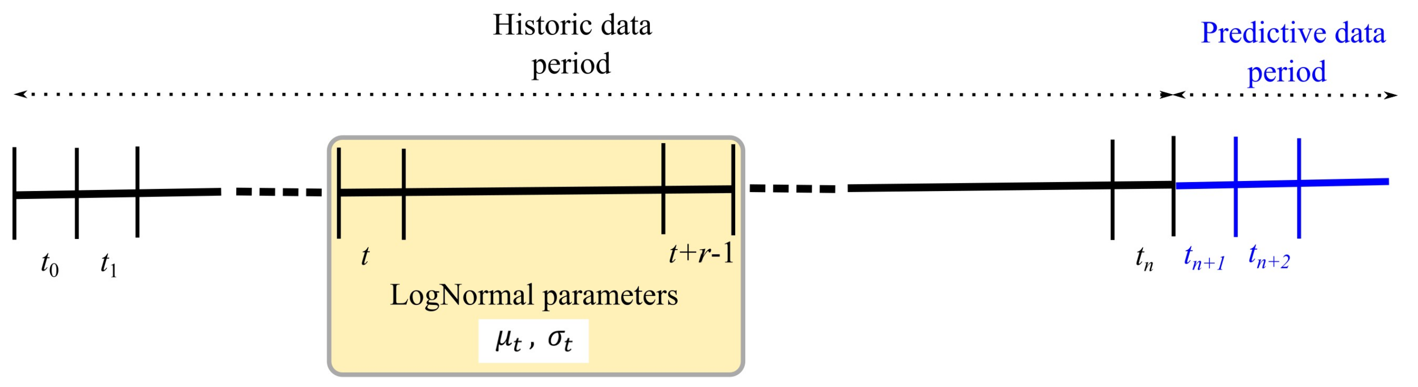
We attempt to predict the future losses using time series derived from historic data. In [33], we found that predicting 3 months into the future was sufficiently accurate in most cases. Therefore, suppose that n quarters are available and that “windows” of r consecutive quarters are taken. Therefore, there are such windows. Then, a window starting at time t with length r quarters ends at quarter . Within that window, we assume that losses are lognormally distributed and can estimate lognormal fit parameters and . The window advances by one quarter at a time. Successive parameter estimations for each window define the time series used for predictions of future data. Figure 1 shows the window starting at time t within the total n quarters.
Algorithm 1 shows the overall FSF process, projecting m quarters into the future.
| Algorithm 1: Forward Stress Framework (FSF) process | |
| |
Parameter Prediction
The last window that can be formed from the historic data spans the period to . The corresponding time series and are then used to predict the next pair of lognormal parameters and . The prediction is made using Loess fits to the and time series plus a “mean reversion” term to counter the trend continuation tendency of Loess. Therefore, if represents the Loess function with span parameter s applied to a time series argument X and is the expected value of the argument X, then we can define a linear combination operator that acts on X. We found that produced credible results. With that operator, the and predictors for quarter are given in Equation (5).
The predictors and can then be used to generate a random sample of lognormally distributed losses for quarter . The sample size is set to the number of days, , in that quarter. Capital can then be calculated for the combination of the losses generated for quarter (which can be stressed), with historic losses from the preceding quarters. The window then advances by one quarter at a time.
3.2. Stress Factor Calculation
It is assumed that historic stress-type values are supplied externally (for example, by a regulatory authority). It is likely that predicted stress type values will also be supplied.
To avoid problems of infinite relative change in a stress type caused by a move from a zero value in the previous quarter, all features are first normalised (on a feature-by-feature basis) to the range [1,10]. The precise range is not important, provided that it does not include zero. To calculate the stress factors in Equation (1), the starting point for stress type j is a time series of m-n values of a stress type j: (with ). Given the stress type values for index j (normalised to [1,10] to avoid division by zero), denote the normalised value stress type by and the normalisation function by . Then, the stress factors are calculated using the first two parts of Equation (6). The product in the third part is the stress factor vector.
3.3. Theoretical Basis of the FSF
The theoretical basis of the FSF is a second order Taylor approximation for capital. In practice, the implementation is encapsulated by Equation (6). Each term in it represents some part of the calculation.
The Taylor expansion is set up in the following way: using an extension of the notation introduced in Section 3 which better fits with the usual “Taylor” notation. Let be the capital at time t for a set of losses x subject to a set of J stress factors . Then, a second-order Taylor expansion of is given by Equation (7), in which denotes all terms of order 3 or more in the increments and .
The first-order term in Equation (7) represents the effect of a change in V due to a change in data. That data change is calculated using the Loess estimators for the period . The result is the term in Equation (4). The two steps are as follows:
- A calculation of the estimated lognormal parameters and , the details of the discrete version of which are in Equation (5). Nominally, is one quarter.
- Generation of a random sample of size lognormal losses using and , where is the number of days in the period .
The first-order term in Equation (7) represents the effect of a change in V due to a time progression of stress. It uses the generated losses and is another two-step process.
- Calculate the stress factor (Equation (6)) .
- Apply the stress in the form .
The second-order terms in Equation (7) represent the effect of a pair of stress types on V. That represents the product of a pair of stress factors in Equation (6). In practice, more than two stress types are possible, and in that case, the interpretation of these second-order terms is a recursive application of product pairs. The second-order partial derivative terms involving time, and are treated as non-material and are not modelled in Equation (6). Similarly, the third- and higher-order terms are also treated as non-material.
Stress Factor Types
The FSF was originally designed to accommodate the economic data provided by the Bank of England [1]. The BoE data is supplied in spreadsheet form, from which stress factors can be derived using the method described in Section 3.2. Consequently, a similar pattern was adopted for data from other sources. The BoE data comprises time series (both historic and predicted) for economic variables such as GDP, unemployment, and oil price for the UK and for other jurisdictions (the EU, the USA, China, etc.). Practitioners can select whichever they consider to be relevant and can add others if they choose. A lower of limit 0.9 can be imposed on stress factor values to prevent excessive “de-stressing”. Similarly, an upper limit of 3.0 prevents excessive stress. In principle, any data series can be used to calculate stress factors, provided that the data are relevant. We have considered, for example, cyber crime using the Javelin database [34,35] and the UK Office for National Statistics [36]. With increasing awareness on climate change, Haustein’s HadCRUT4-CW (Anthropogenic Warming Index) data [37] on global warming are available. In practice, global warming stress factors are only marginally greater than 1 and thus supply virtually no stress in the short term.
OpRisk scenarios are usually expressed in “Impact-Horizon” form, such as an impact of 50 million and a horizon of 25 years. This would normally be expressed as “50 million, 1-in-25”. To fit the FSF paradigm, this format must be translated to the required stress factor format (Equation (6)). Appendix C suggests a method to do that by calculating a probability that, for a 1-in-H scenario with impact M, there will be at least one loss of value M or more in the next H years.
In order to test particular stress scenarios, the format of the stress factor makes it easy to define user-defined stress factors. To test an annual scenario in which model parameters are changed by a factor , the approximation is a reasonable starting point for the required single quarter stress factor. As an illustration, the results for an extreme economic stress scenario is given in Section 4.2.1.
Stress factors that manipulate data directly can also be accommodated. Dedicated programming is the simplest way to accomplish this task, although it is possible to supply suitable formulae in a spreadsheet. Appendix B shows how it can be done. The results for an example in which only the largest losses are scaled is given in Section 4.2.1.
3.4. Choice of Distribution
The analysis in the preceding sections has concentrated on the LogNormal distribution. In principle, an alternative fat-tailed distribution could be used. The issue of which to use is not simply a matter of using a best-fit distribution. Some distributions provide better differentiation between predicted losses under “no stress” and stressed economic conditions. That is largely due to the value of the empirical standard deviation in a series of identical runs. The principal source of variation is the stochastic components inherent in the FSF. The LogNormal distribution has several advantages. The empirical standard deviation in a series of identical runs is small compared to some others (Pareto, for example). Therefore, it is possible to note that a mildly stressed economic case does result in a corresponding mildly inflated capital when compared to applying no stress.
In practice, the evaluation of LogNormal distribution parameters and ordinates is fast and reliable. Instances of failure to converge in parameter estimation are extremely rare. The Pareto (in our case, the type I variety) distribution is particularly notable because it tends to produce a significantly higher VaR than most others. Therefore, a Pareto distribution is unlikely to be a good predictor of future capital. However, if used as a discriminator between predictions using stresses and unstressed losses, it has potential. Section 4.3 contains an evaluation of commonly used fat-tailed distributions.
4. Results
The results for predictions and correlations follow the notes on data and implementation.
4.1. Data and Implementation
Two OpRisk loss data sets were used. The first was extracted from a dedicated OpRisk database and spans the period from January 2010 to December 2019. The Basel risk class CPBP was excluded because of distortions introduced by extreme losses and in accordance with BoE directives. We refer to it as nonCPBP. The second is a control data set, randomly generated from a lognormal (10,2) distribution. control has one simulated total loss per day for the same period.
Of the supplied BoE economic stress types, the following were considered “relevant”. Lagged variables were not used.
- UK.Real.GDP; UK.CPI; UK.Unemployment.Rate;
- UK.Corporate.Profits; UK.Residential.Property; UK.Equity.Prices;
- Bank.Rate; Sterling.IG.Corp.Bond.Spread; Secured.Lending.Individuals;
- Consumer.Credit.Individuals; Oil.Price;
- Volatility.Index; GBPEUR; GBPUSD.
All are used with two sets of economic data supplied by the BoE. Base data were intended to model mild stress, and ACS (Annual Cyclical Scenario) was intended to model more severe (but not extreme) stress. In addition, an extreme data set was proposed to model extreme economic conditions such as mass unemployment, negative GDP, and severely reduced household income. The COVID-19 scenario models the (surprising) effect on OpRisk losses in the period January–July 2020. There is evidence, from Risk.net [38], that there has been a 50% reduction in OpRisk losses. This is attributed to much reduced transaction volumes. Some increase in fraud was noted, with a slight increase in customer complaints due to Internet and bank branch access problems. The COVID-19 scenario was constructed using simulated transaction levels that represent a 50% reduction in transaction volume in year 1, rising to 70% in year 2.
All calculations were conducted using the R statistical programming language (https://www.r-project.org/ (accessed on 6 January 2021)), with particular emphasis on the lubridate and dplyr packages for date manipulation and data selection, respectively. Mathematica version 12 was used for graphics and dynamic illustrations.
4.2. Forward Stress Framework Results
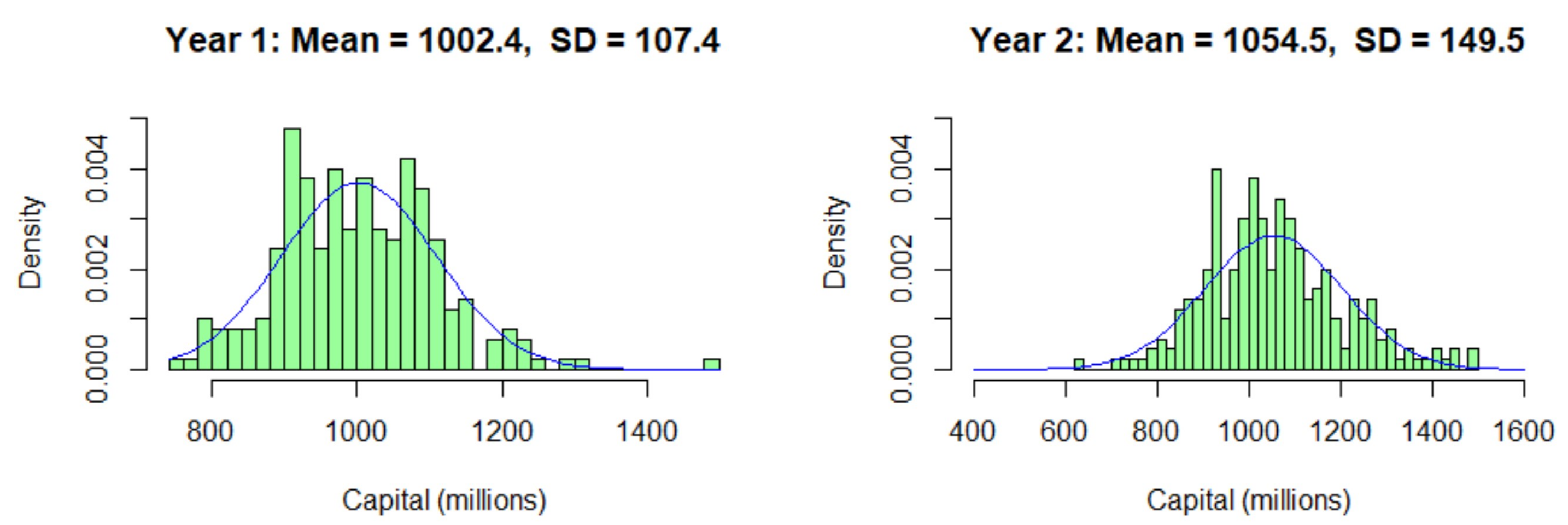
Table 1 gives the mean (m) and standard deviation (s) of 25 independent runs in which 1-year and 2-year predictions are made for the nonCPBP and control data under the base and ACS economic scenarios. Empirically, the resulting capital distributions are normally distributed (Figure 2 shows an example); therefore, 95% confidence limits may be calculated using . As a rough guide, the confidence limits vary from the means by about 25% for nonCPBP and 17% for control.
4.2.1. Forward Stress Framework Predictions
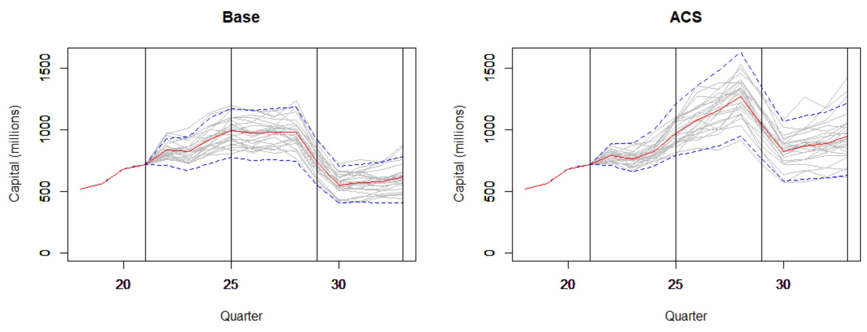
Figure 3 shows 25 sample paths (from 250 simulations) for the nonCPBP data using the base and ACS economic data. This gives an idea of the spread of predictions. The two path profiles are similar, with an approximately constant spread over the two-year period for the base case. The ACS plot shows greater volatility with increasing time as well as an expected higher general capital level.
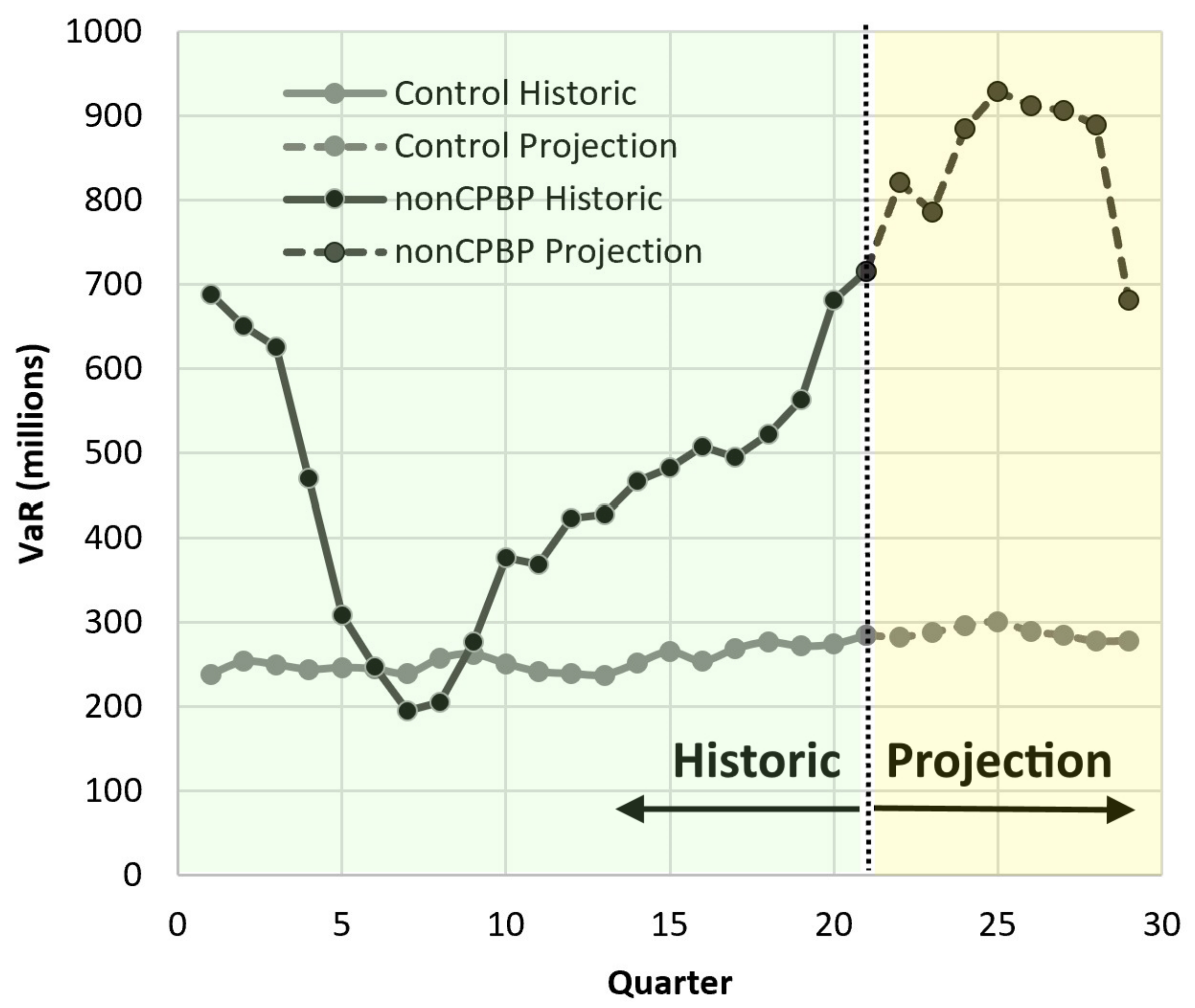
Figure 4 shows the nonCPBP historic data and the control data with 2-year predictions under no stress (i.e., all stress factors are set to 1). The marked variation in the historic nonCPBP data is notable and reflects changes in data collection methods as well as in losses incurred.
4.2.2. Projections: Economic and Scenario Stress
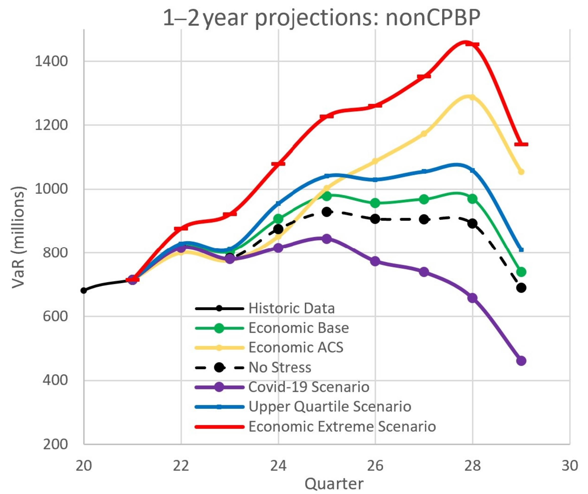
In this section we show the projection results for both the nonCPBP and control data sets under BoE’s economic stress scenarios (base and ACS). Two scenario projections are also shown. The extreme scenario models a severe downturn in economic conditions, much harsher than conditions implied by the ACS case. It was derived by exaggerating ACS data. The stress factors for the base, ACS, and extreme cases were calculated using Equation (6). The upper quartile scenario models an extreme condition by inflating the largest losses by 25%. The largest losses are known to have a significant effect on regulatory capital (see [8]). Technically, the stress factors in the upper quartile were supplied by reading a spreadsheet containing instructions to manipulate selected losses in the way required. Figure 5 shows the 2-year nonCPBP projection details (quarters 21–29) for all cases. The downward trend for the COVID-19 scenario and the steep rise in the extreme economic scenario are both highly prominent.
The plots in Figure 5 illustrate an inherent volatility in the historic data. In all cases, the predicted profiles have the same shape and the base case effect is small. The ACS case is only significant effect in year 2. The extreme scenario is much more pronounced than the upper quartile scenario, in which only the most extreme losses are inflated. The downward trend for the COVID-19 scenario only becomes marked in the second year.
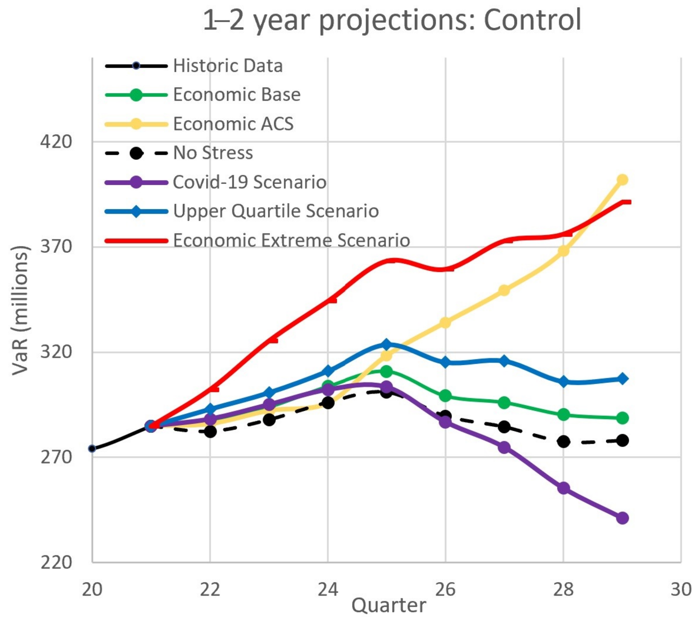
Figure 6 shows the equivalent projections for the control data. Those plots give a better understanding of the effect of the various economic cases, since the “historic” data profile is essentially non-volatile. The profiles follow the same pattern as for the nonCPBP data.
Table 2 shows a three-year summary in terms of percentage changes relative to a “no change” state for the base, ACS, extreme, and COVID-19 cases. For the first year only, a mild increase is indicated, effectively showing that the BoE’s economic projections are relatively modest.
Appendix A shows a further view of the nonCPBP projections in the form of confidence surfaces. Appendix D shows a first-order approximation for the confidence bounds for capital, implemented in symbolic terms using Mathematica. The results show that those confidence bounds are well-conditioned with respect to the stress factor parameter, .
4.2.3. The Effect of Global Warming
4.3. Results Using Other Distributions
To test the effect of distributions other than LogNormal on the FSF, the analysis in Section 3 was repeated, substituting a range of alternative distributions for the LogNormal. It is well known in OpRisk circles that, even if more than one distribution fits the data (in the sense that a goodness-of-fit test is passed), the calculated capitals can be very different. Therefore, two comparisons were made. First, the percentage changes in calculated capitals under stressed and unstressed conditions after 1 and 2 years were noted. Second, the 5-year data windows in Figure 1 were tested for goodness-of-fit (GoF) to selected distributions.
The criteria to be evaluated for each distribution tested are as follows:
- Does the model predict a sufficient distinction between the “no stress” case and stresses due to the base and ACS scenarios in both 1 and 2 years?
- As many as possible data sets tested should pass an appropriate GoF test.
- Are predicted capitals consistent with the capital calculated using empirical losses only. We expect capitals predicted using a distribution to be greater than the capitals calculated using empirical losses only, since the empirical capital is limited by the maximum loss. Capitals calculated from distributions are theoretically not bounded above. However, they should not be “too high”. As our “rule of thumb”, 5 times the empirical capital would to “too high”.
Table 4 shows the results of a comparison of predictions in the ’no stress’, base, and ACS cases.
Table 4 shows that the LogNormal and Weibull distributions both provide a reliable and sufficient distinction between stressed and unstressed conditions. They also provide accurate parameter estimates and run quickly. The LogNormal year 2 prediction is much larger than the Weibull equivalent, as might be expected from severe stress. However, year 2 predictions are less reliable for all distributions.
The response from GoF tests shows that LogNormal fits are the most appropriate. Twenty-one 5-year windows are available in the construct summarised in Figure 1, and the TNA GoF test was applied to each. Details of the TNA test may be found in [5]. This test was formulated specifically for OpRisk data and has two main advantages over alternatives. First, it is independent of the number of losses. Second, the value of the test statistic at confidence level c%, , provides a very intuitive measure of GoF and the value of is a direct measure of the quality of the fit. Zero indicates a perfect fit. The 5% 2-tailed critical value is 0.0682. Therefore, values of in the range (0, 0.0682) are GoF passes at 5%.
Table 5 shows a comparison of the GoF statistics for the range of fat-tailed distributions tested. The values presented show that the LogNormal distribution is a very good fit for all 21 of the 5-year periods, and that other distributions are viable. In particular, the Gamma and LogGamma distributions are also good fits for all of those periods. Others are poorer fits, either because of the number of satisfactory fits or the GoF themselves. The mean TNA value for the Gamma distribution exceeds the mean TNA value for the LogNormal, making it less preferable. Although the mean TNA value for the LogGamma distribution is less than the corresponding LogNormal value, 13 of the 21 LogNormal passes were also significant at 1%, compared with only 3 for LogGamma. The column “Consistency with Empirical VaR” shows whether the VaR estimates are “too small” or “too large” (criterion 3 at the start of this subsection). Distributions that produce “too small” or “too large” VaRs can be rejected. In addition, parameter estimation for LogNormal distributions is much more straightforward than for LogGamma distributions. Therefore LogNormal is the preferred distribution.
Therefore, the LogNormal distribution is optimal for use in the FSF because it provides a best fit for the empirical data and provides an appropriate distinction between the unstressed and stressed cases.
4.4. Correlation Results
Correlations between economic indicators (quoted quarterly) and nonCPBP OpRisk losses (quarterly loss totals) were assessed using Spearman rank correlation, which is more suitable if the proposed regression relationship is not known to be near-linear. The statistical hypotheses for the theoretical correlation coefficient were null, , and alternative, . The list below shows the results.
- There were 15 economic indicators.
- Only one (UK.CPI) was significantly correlated (at 95% significance) with nonCPBP loss severity.
- Only two (Bank.Rate and Volatility.Index) were not significantly correlated with nonCPBP loss frequency.
- Eleven significant frequency correlations were at a confidence level of 99% or more.
- Two significant frequency correlations were at a confidence level of between 95% and 99%.
The explanation of these results is straightforward. Many of the historic economic time series show a marked trend with respect to time. Similarly, the aggregated loss frequency time series do too. In contrast, the aggregated severity-based time series do not. Associating two trending series inevitably results in a significant correlation.
Correlation Persistence
The conclusion from the literature review in Section 2 was that, if correlations between economic factors and OpRisk losses exist, they do not persist. We can confirm that conclusion using our data. With a rolling window of length five years, Spearman’s rank correlation coefficient was calculated for the five-year periods corresponding to start quarters 1, 2, …, 21, and 14 economic factors. A total of 294 correlations were examined.
Table 6 shows that only a small percentage of severity correlations persist for 5 years, whereas a high percentage of frequency correlations do. Correlations therefore depend critically on the time period selected. The two severity correlations that are significant both occur within the five-year periods starting at quarters 1 and 2. In that period, data collection was less reliable than it was in later quarters. The significant frequency correlations are more numerous in the five-year periods starting at quarters 8 and 9, which was when a marked decrease in loss frequency started to become most apparent. The correlations that exist are due to associating pairs of trending time without any explicit justification for those associations.
4.5. Inappropriate Correlations
We caution against calculating correlations of OpRisk losses with potential stress types for which no relationship with those losses is apparent. Many can be found in the World Bank commodity database [39], and many of them have significant correlations with the nonCPBP severity data. The following commodities were correlated with the nonCPBP OpRisk losses at 5%: agricultural raw materials; Australian and South African coal; and Australian and New Zealand beef, lamb, groundnuts, sugar, uranium, milk, and chana. Furthermore, the commodity data for aluminium and cotton were positively correlated at 1% significance with the same nonCPBP data. The variety and number of commodities in these lists indicate, possibly, that there is some sort of underlying factor, as yet unknown. Twelve out of 85 significant correlations are many more than would be expected at 5% confidence. One would expect 5% of .
5. Discussion
Overall, OpRisk losses are event-driven and are subject to particular economic shocks. Consequently, and perhaps conveniently, the need to look for correlations between OpRisk losses and stress types can be removed. A general principle should be to only seek correlations if causal factors can be identified. Therefore, doubt must be cast on the validity of the Fed’s CCAR model [29], which uses correlations between loss severity and economic factors to predict regulatory capital.
The Basel Committee has recently issued further guidance on measuring the resilience of the banking system to economic shock [40], largely in response to the COVID-19 pandemic. Whilst the general measures proposed (robust risk management, anticipation of capital requirement, vulnerability assessment, etc.) are sensible, that guidance remains notable in that it continues to not say how capital should be calculated. The proposed FSF method enables capital to be calculated as a quantified response to economic or other data. Although the COVID-19 pandemic represents a very severe economic downturn, indications are that it will not inflate OpRisk losses. Using calculated OpRisk capital for another purpose represents a significant departure from accepted practice in financial risk. Hitherto, the reserve for each risk type has been applied only to that risk type. For financial prudence, we recommend a pooling of reserves, each calculated independently in response to external conditions.
In Section 4.4, we established that very few significant 5-year severity correlations between OpRisk losses and economic factors can be found. Those that do exist do not persist. This finding is sensitive politically since the US CCAR process depends on the existence of such severity correlations. Informally, national regulatory authorities imply that correlations do exist by supplying economic data in the context of financial risk regulation. It is possible that a significant and persistent correlation can be found for an aggregation of all national OpRisk loss severities with economic factors. However, such aggregations are only known to national regulatory authorities, and they would not disclose the data. Regulations do not dwell on loss frequencies, which are explainable, provided that risk controls become increasingly stringent.
5.1. Economic Effects of Operational Risk: Intuitions
The economic effects on operational risk are not always clear. That is the fundamental reason for the detection of only sporadic OpRisk/economic factor correlations. The reasons for this are that OpRisk losses are driven by physical events, behavioural factors, and policy decisions. Causal relationships can be suggested but are not backed by evidence. The examples below illustrate these points.
DPA could increase with social unrest in stressed economic circumstances, but correlations have not been observed. Damage to cabling because of building work, fire, or flooding is much more likely. The same applies for other event-driven risk classes. BDSF, for example, is more likely to be affected by software problems. Anecdotal evidence suggests that EF (but not IF) does increase in stressed economic circumstances. The suggested reason is that fraudsters spot more opportunities. Informally, the amount of fraud can be governed solely by the extent of anti-fraud measures. Some is tolerated because customers disapprove of anti-fraud measures that are too severe. The same principle applies to CPBP and EPWS, which are largely controlled by a bank’s response to customers and employees. CPBP and EPWS are driven by the bank’s operational procedures (such as the number of telephone operators employed) and its policies (such as its response to illegal activity).
The COVID-19 pandemic has had a very significant effect on economic indicators, but the effects on OpRisk losses will not become apparent until the first quarter of 2021. It is likely that provisions will be put in place for safety measures in bank branches and for IT infrastructure to enable “working from home”. Economic scenarios for stress testing that incorporate COVID-19 effects will probably appear in early 2022.
5.2. Overall Assessment of the FSF
The following list is a brief summary of the advantages and disadvantages of our proposed framework.
- Advantages:
- (a)
- It is flexible: stress factors can be added or removed easily.
- (b)
- Correlation is not assumed.
- (c)
- Using projected losses eliminates idiosyncratic shocks since it assumes a “business as usual” environment.
- (d)
- Generating projected losses allows for modification of all or some of the projected losses, which is more flexible than modifying single capital values.
- (e)
- The degree of stress for any given stress type can be geared to achieve any (reasonable) required amount of retained capital. This is an objective way to calculate capital, based on factors that could affect capital.
- (f)
- The framework is able to detect the relative effects of the stress types considered. Some have little effect (e.g., global warming), whereas others have a significant effect (e.g., increasing the largest loss).
- Disadvantages:
- (a)
- It is not entirely straightforward to include stresses that act on parts of the projected data only. Specialised procedures must be used to generate the necessary stress factors.
- (b)
- Generating projected losses requires a loss frequency of approximately 250 per year. Accuracy is lost with fewer losses. For that reason, the aggregate risk class nonCPBP was used to obtain an overall view of the effect of stress.
- (c)
- Special treatment is needed for stresses that have a decreasing trend with time but are thought to increase capital. Decreasing stress values would result in stress factors that are less than 1. We suggest replacing a stress factor by in such cases. Stresses in this category have to be identified in advance of calculating stress factors.
- (d)
- There is no objective way to decide what stress types should be used.
5.3. Guidance for Practitioners, Modellers, and Regulation
The results presented in Section 4.2, Section 4.2.1, and Section 4.2.2 have highlighted points of note for regulation, for modelling, and in practice.
5.3.1. Regulation
European regulators are unlikely to specify precisely how stress testing should be conducted, and the Fed is unlikely to change its overall approach to the CCAR process. However, regulators can note that significant correlations cannot always be found. European banks are therefore likely to remain free to implement whatever stress testing method they deem appropriate. The FSF provides such a method that avoids explicit use of non-significant correlations.
5.3.2. Modelling
A primary issue is fitting a distribution to data. Typically, distribution parameters are often calculated using the Maximum Likelihood method. The major problems are in estimating suitable initial parameters values, speed of convergence, and failed convergence (in which case, initial estimates have to be used). Alternative parameter calculation methods sometimes result in very different parameter values. An example is the R packages Pareto and EnvStats, both of which can be used to model a Pareto distribution. The latter is very slow and can provide parameter values that result in VaR values that are many orders of magnitude greater than the largest empirical losses.
A further problem to be avoided is that some distributions can generate huge losses in random samples that skew VaR upwards to such an extent that they completely dominate the VaR. This problem occurs for the Pareto, LogLogistic, and G&H distributions and is exacerbated in small samples. A solution is to detect and remove those items from the sample.
5.3.3. Practice
If model parameter choices are left to practitioners, details such as which distribution and how many Monte Carlo cycles to use can affect results. If those questions are answered automatically, practitioners should be aware that producing curves such as in Figure 5 and Figure 6 is time-consuming. Repeat runs are needed to obtain consistent results, and we recommend at least 25, for which several hours is likely to be needed. Practitioners should also note the spread of predictions and always report results in terms of confidence bounds (similar to those in Figure 3). They should also be aware of two further points. First, long-term predictions are less reliable than short-term predictions. Second, the choice of stress data (economic, fraud, etc. or user-defined) must be appropriate.
6. Conclusions
The principal conclusions are as follows:
- Predictions of OpRisk capital based on economic factor correlations is unsafe, as statistically significant correlations do not always exist. The proposed FSF provides a viable alternative to naive use of correlations in the context of OpRisk/Economic factor stress testing.
- The FSF works by calculating stress factors based on changes in economic factors (or any other stress type) and by applying them to projected OpRisk losses. As such, it acknowledges that OpRisk capital should increase in response to economic stress.
- The FSF is flexible and responsive. It allows for investigation using appropriate time series (not only the BoE economic data) as well as using user-defined scenarios.
- FSF has a disadvantage in that it requires a minimal volume of data to generate the necessary samples and predictions. Therefore, using individual Basel risk classes is not always feasible.
Further Work
Further work on reverse stress testing is already well-advanced and uses the same sampling and prediction techniques that were described in the FSF algorithm (see Algorithm 1). Suitable risk factors can be found quickly and reliably using a binary search as well as Bayesian optimisation. We also expand the suggestion in Appendix C to cast OpRisk scenarios from their usual “severity + horizon” form to the stress factor format used in the FSF.
Funding
This research received no external funding.
Institutional Review Board Statement
Not applicable.
Informed Consent Statement
Not applicable.
Conflicts of Interest
The author declares no conflict of interest.
Appendix A. Upper and Lower Confidence Surfaces
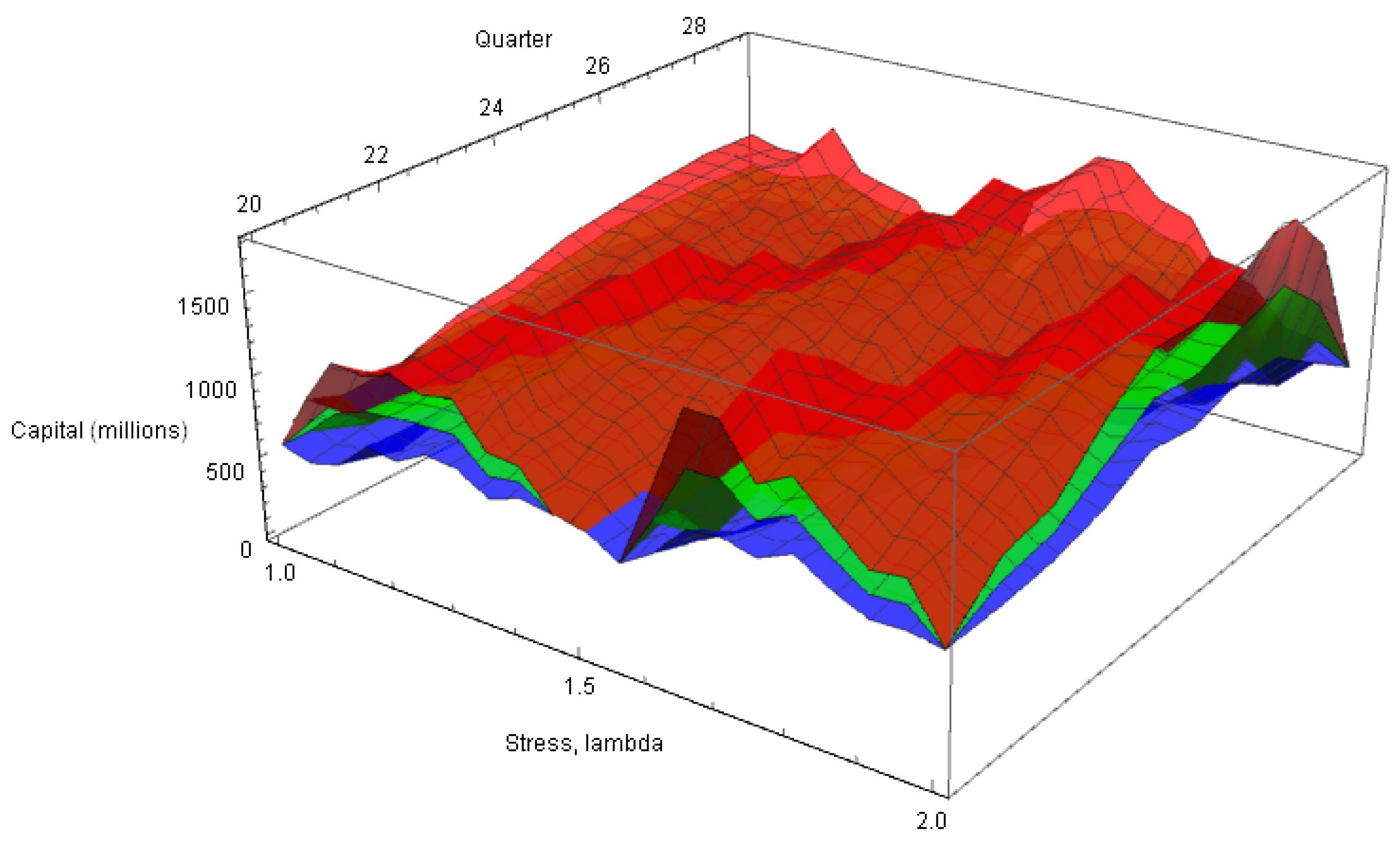
Figure A1 shows upper and lower confidence surfaces for the 2-year capital projections using the FSF. Each surface comprises a projected capital calculation for particular values of a stress factor (representing zero to 100 per cent stress) and a quarter. The main features are listed below.
- Very uneven surfaces due to data volatility.
- Increasing capital with increasing time, apart from quarters 27 and 28, when there were much reduced losses.
- Small overall increases in capital with increasing stress.
- Non-divergent upper and lower confidence surfaces, indicating a stable stochastic error component.
Figure A1.
NonCPBP 95% confidence surfaces based on samples of size 10 for each point on each surface: upper (red), lower (blue), and mean (green).
Figure A1.
NonCPBP 95% confidence surfaces based on samples of size 10 for each point on each surface: upper (red), lower (blue), and mean (green).

Appendix B. Stress Factor Produced by Using a Supplied Formula
This appendix shows how a stress factor may be supplied via a text-based formula, which is interpretable by a host program (in this case, R). The intention is to “deliver” the formula using a spreadsheet, text, or database, organised as a list of items, one for each quarter. The formula should specify a multiplier for each datum generated in the FSF predictive stage. In this case, the data in the upper quartile are scaled by a specified scale factor (1.5, a 50% increase), and the data in the three lower quartiles are left unchanged. Two reserved variable names are used in the formula: DATA and STF. They are local variables in the host program and are instantiated when the formula is interpreted. DATA is a reference to the generated data , and STF is a reference to the required stress factor.
The required formula is a concatenation of three lines of code, condensed into a single line (the lines are separated here to make them more easily readable):
- sf.1 <- replicate( floor(0.25∗length(DATA)), 1.5);
- sf.2 <- replicate(length(DATA) - floor(0.25∗length(DATA)), 1);
- STF <- c(sf.1,sf.2)
Having read all formulae into a variable Formula_Q4, (which is a data table with two columns, Quarter and Scale), the revised code below instantiates the formula for quarter qtr. Using the construct Formula_Q4[Formula_Q4\$Quarter==qtr,] gives a great deal of flexibility because a different formula can be supplied for each qtr. All that is required is to vary the scale factor 1.5.
- txt <- "DATA <- sort(DATA, decreasing = T); " # sort DATA
- # Read formula
- txt <- paste(txt, Formula_Q4[Formula_Q4$Quarter==qtr,], sep="")
- # Evaluate formula and to output STF
- eval(parse(text = txt))
Appendix C. Scenario-Defined Stress Factors
This appendix describes a method of converting a scenario expressed in terms of an impact M and a time horizon H into a stress factor for use in the FSF. An example is an impact of 50 (million USD) with a horizon of 1-in-25 (years), meaning that, in the next 25 years, at least one loss of 50 million USD or more is anticipated.
Suppose, further, that the scenario is used with n losses spanning a period y years. Isolate the set of losses that exceed , where is a scale factor that ensures that said set is not empty. Denote the number of elements in that set by . Next, calculate a parameter , which is the expected number of losses that exceeds in the time window of y years. That number serves as a parameter for a Poisson model (Equation (A1)).
Then, the Poisson probability p that there will be at least one loss of impact M in the horizon period H is
The probability p can then be expressed as a quarterly (hence the factor 4) stress factor by calculating
The same value should then be used at each time step in the FSF process.
Appendix D. Sensitivity of Capital with Respect to the Stress Factor
Symbolic computation can be used effectively to study the sensitivity of capital with respect to the stress factor, which is controlled by the parameter of Equation (6). In particular, we consider the confidence bounds of Appendix A. In order to simplify the notation slightly, the subscript t in the stress factor is omitted in what follows. It should be understood that the symbol “” refers to the stress factor applied at some time t and that the same applies for other parameters introduced.
Rao [41] has shown that, if Q is a random variable that represents an observation q of the quantile of a distribution with density derived from a sample of size n, then Q has a normal distribution given by Equation (A4).
Therefore, the upper and lower symmetric c% confidence bounds are given, respectively, by (where is the appropriate normal ordinate for the percentage point c, for example 1.96 when c = 95%):
It is easy to derive symbolic first-order approximations for and . For a small change, in , the corresponding first order changes in and are as follows:
Now consider the case of a random variable that has a lognormal mixture distribution with mixture parameter r and density ( is the normal density function). This density corresponds to the control data, discussed in Section 4.1.
Using Mathematica, if the Rao variance (Equation (A4)) is defined in a procedure Rao[m_, s_, lambda_, r_, u_, n_, p_], then the implementation of Equations (A5) and (A6) is as follows:
- R = Rao[m, s, lambda, r, u, n, p]
- CU = q + zc R
- dCU = dlambda D[CU, lambda]
- CL = q - zc R
- dCL = dlambda D[CL, lambda]
The expressions for and derived in Mathematica are summarised in Equation (A7). Both and are dominated by the additive term q.
The Mathematica expressions for and are not palatable. They are dominated by the expressions in Equation (A8), arising from . Since and q are constant, and . In Equation (A8), and h are the same as in Equation (A7).
The right-hand-most bracket gathers all terms that contain the parameter and, therefore, determines the -variation of and, hence, of and . With parameter values consistent with those normally observed, the components of are of the following orders.
- Left-hand-most term
- Middle term
- Right-hand-most term
Overall, or , depending on the value of . This term is several orders of magnitude less than the magnitude of and (typically ). Therefore, and especially if is small, the incremental derivative component makes only a marginal change to the capital confidence limits. Consequently, and are well-conditioned with respect to .
References
- Bank of England. Stress Testing. Available online: https://0-www-bankofengland-co-uk.brum.beds.ac.uk/stress-testing (accessed on 16 December 2020).
- European Central Bank. 2020 EU-Wide Stress Test—Methodological Note. Available online: https://eba.europa.eu/documents/10180/2841396/2020+EU-wide+stress+test+-+Draft+Methodological+Note.pdf (accessed on 16 December 2020).
- US Federal Reserve Bank. Dodd-Frank Act Stress Test 2019: Supervisory Stress Test Methodology. Available online: https://www.federalreserve.gov/publications/files/2019-march-supervisory-stress-test-methodology.pdf (accessed on 16 December 2020).
- Basel Committee on Banking Supervision. International Convergence of Capital Measurement and Capital Standards, Clause 644. Available online: https://www.bis.org/publ/bcbs128.pdf (accessed on 8 February 2021).
- Mitic, P. Improved Goodness-of-Fit Tests for Operational Risk. J. Oper. Risk 2015, 15, 77–126. [Google Scholar] [CrossRef]
- Jorion, P. Value at Risk: The New Benchmark for Managing Financial Risk, 3rd ed.; McGraw Hill: New York, NY, USA, 2007. [Google Scholar]
- Basel Committee on Banking Supervision. QIS 2: Summary of Results. Available online: https://www.bis.org/bcbs/qis/qisresult.htm (accessed on 16 December 2020).
- Mitic, P. Conduct Risk: Distribution Models with Very Thin Tails. In Proceedings of the 3rd International Conference on Numerical and Symbolic Computation Developments and Applications (SYMCOMP 2017), Guimarães, Portugal, 6–7 April 2017. [Google Scholar]
- Mitic, P.; Hu, J. Estimation of value-at-risk for conduct risk losses using pseudo-marginal Markov chain Monte Carlo. J. Oper. Risk 2019, 14, 1–42. [Google Scholar] [CrossRef]
- Frachot, A.; Georges, P.; Roncalli, T. Loss Distribution Approach for Operational Risk. Available online: http://ssrn.com/abstract=1032523 (accessed on 16 December 2020).
- Baudino, P.; Goetschmann, R.; Henry, J.; Taniguchi, K.; Zhu, W. FSI Insights on Policy Implementation No 12: Stress-Testing Banks—A Comparative Analysis. Available online: https://www.bis.org/fsi/publ/insights12.pdf (accessed on 16 December 2020).
- Blaschke, W.; Jones, M.; Majnoni, G.; Peria, S. Stress Testing of Financial Systems: An Overview of Issues, Methodologies, and FASP Experiences. Available online: https://www.imf.org/external/pubs/ft/wp/2001/wp0188.pdf (accessed on 16 December 2020).
- Basel Committee on Banking Supervision. Amendment to the Capital Accord to Incorporate Market Risks. Available online: www.bis.org/publ/bcbs24.pdf (accessed on 17 December 2020).
- Basel Committee on Banking Supervision. Stress Testing Principles. Available online: https://www.bis.org/bcbs/publ/d450.pdf (accessed on 17 December 2020).
- Axtria Inc. Portfolio Stress Testing Methodologies. Available online: https://insights.axtria.com/whitepaper-portfolio-stress-testing-methodologies (accessed on 3 October 2020).
- Drehmann, M. Macroeconomic stress-testing banks: A survey of methodologies. In Stress-Testing the Banking System: Methodologies and Applications; Cambridge University Press: Cambridge, UK, 2009. [Google Scholar]
- Grundke, P. Reverse stress tests with bottom-up approaches. J. Risk Model Valid. 2011, 5, 71–90. [Google Scholar] [CrossRef] [Green Version]
- Rebonato, R.; Denev, A. A Bayesian Approach to Stress Testing and Scenario Analysis. J. Investig. Manag. 2010, 8, 1–13. [Google Scholar]
- De Fontnouvelle, P.; DeJesus-Rueff, V.; Jordan, J.S.; Rosengren, E.S. Capital and Risk: New Evidence on Implications of Large Operational Losses. J. Money Credit Bank. 2006, 38, 1819–1846. [Google Scholar] [CrossRef] [Green Version]
- Allen, L.; Bali, T. Cyclicality in catastrophic and operational risk measurements. J. Bank. Financ. 2006, 31, 1191–1235. [Google Scholar] [CrossRef] [Green Version]
- Moosa, I. Operational risk as a function of the state of the economy. Econ. Model. 2011, 28, 2137–2142. [Google Scholar] [CrossRef]
- Cope, E.W.; Antonini, G. Observed correlations and dependencies among operational losses in the ORX consortium database. J. Oper. Risk 2008, 3, 47–74. [Google Scholar] [CrossRef]
- Cope, E.W.; Piche, M.T.; Walter, J.S. Macroenvironmental determinants of operational loss severity. J. Bank. Financ. 2012, 36, 1362–1380. [Google Scholar] [CrossRef]
- Cope, E.W.; Carrivick, L. Effects of the financial crisis on banking operational losses. J. Oper. Risk 2013, 8, 3–29. [Google Scholar] [CrossRef]
- Bank of England. Financial Stability Report June. Available online: www.bankofengland.co.uk/financial-stability-report/2018/june-2018 (accessed on 18 December 2020).
- Bank of England. Financial Stability Report, Financial Policy Committee Record and Stress Testing Results—December 2019. Available online: https://0-www-bankofengland-co-uk.brum.beds.ac.uk/financial-stability-report/2019/december-2019 (accessed on 18 December 2020).
- Bank of England. Interim Financial Stability Report May 2020. Available online: https://0-www-bankofengland-co-uk.brum.beds.ac.uk/-/media/boe/files/financial-stability-report/2020/may-2020.pdf (accessed on 18 December 2020).
- Curti, F.; Migueis, M.; Stewart, R. Benchmarking Operational Risk Stress Testing Models. Available online: https://0-doi-org.brum.beds.ac.uk/10.17016/FEDS.2019.038 (accessed on 18 December 2020).
- US Federal Reserve Bank. Stress Tests and Capital Planning: Comprehensive Capital Analysis and Review. Available online: https://www.federalreserve.gov/supervisionreg/ccar.htm (accessed on 18 December 2020).
- Klugman, S.A.; Panjer, H.H.; Willmot, G.E. Loss Models, 2nd ed.; Wiley: New York, NY, USA, 2004. [Google Scholar]
- Hassani, B.K. Scenario Analysis in Risk Management; Springer: Cham, Switzerland, 2016. [Google Scholar]
- Risk.net. Stress-Testing Special Report. Available online: https://www.risk.net/stress-testing-special-report-2020 (accessed on 15 February 2020).
- Mitic, P.; Bloxham, N. A Central Limit Theorem Formulation for Empirical Bootstrap Value-at-Risk. J. Model Risk Valid. 2018, 12, 1–34. [Google Scholar] [CrossRef]
- Pascual, A.; Marchini, K.; Miller, S. Identity Fraud: Fraud Enters a New Era of Complexity. Available online: https://www.javelinstrategy.com/coverage-area/2018-identity-fraud-fraud-enters-new-era-complexity (accessed on 20 December 2020).
- Tedder, K.; Buzzar, J. 2020 Identity Fraud Study: Genesis of the Identity Fraud Crisis. Available online: https://www.javelinstrategy.com/coverage-area/2020-identity-fraud-study-genesis-identity-fraud-crisis (accessed on 20 December 2020).
- UK Office for National Statistics. Crime in England and Wales: Appendix Tables (Table A4 Computer Fraud). Available online: https://www.ons.gov.uk/peoplepopulationandcommunity/crimeandjustice/datasets/crimeinenglandandwalesappendixtables (accessed on 20 December 2020).
- Haustein, K.; Allen, M.R.; Forster, P.M.; Otto, F.E.L.; Mitchell, D.M.; Matthews, H.D.; Frame, D.J. A Real-Time Global Warming Index. Sci. Rep. 2017, 7, 15417. [Google Scholar] [CrossRef] [Green Version]
- Risk.net. Op Risk Data: Losses Plummet During Lockdown (ORX News). Available online: https://www.risk.net/comment/7652866/op-risk-data-losses-plummet-during-lockdown (accessed on 20 December 2020).
- World Bank. Commodities Markets. ’Pink Sheet’ Data Monthly. Available online: https://www.worldbank.org/en/research/commodity-markets (accessed on 20 December 2020).
- Financial Stability Institute: Bank for International Settlements. Covid-19 and Operational Resilience: Addressing Financial Institutions’ Operational Challenges in a Pandemic. Available online: https://www.bis.org/fsi/fsibriefs2.pdf (accessed on 20 December 2020).
- Rao, C.R. Linear Statistical Inference and Its Applications, 2nd ed.; Wiley-Interscience: Hoboken, NJ, USA, 2009. [Google Scholar]
Figure 1.
Time line showing a window of length r quarters in n quarters of historic data. The yellow highlight shows a window spanning the period t to , for which the fitted lognormal parameters are and . Windows that use only historic data are indicated in black, and windows that use some predicted data are indicated in blue.

Figure 2.
Histograms of 1- and 2-year nonCPBP predictions using the ACS scenario, showing fitted normal curves. The corresponding histograms for the base scenario are similar.
Figure 2.
Histograms of 1- and 2-year nonCPBP predictions using the ACS scenario, showing fitted normal curves. The corresponding histograms for the base scenario are similar.

Figure 3.
One- and two-year nonCPBP sample paths for the base and ACS economic scenarios. The mean path is shown in red, and 95% symmetric confidence bounds are shown in blue. The vertical lines are set at prediction inception (quarter 21) and at the 1- and 2-year future predictions (quarters 25 and 29, respectively).

Figure 4.
Historic nonCPBP and control data with 1- and 2-year Loess projections under no stress: Historic data (left of the vertical line) is shown in green, and projected data (right of the vertical line) is shown in yellow.
Figure 4.
Historic nonCPBP and control data with 1- and 2-year Loess projections under no stress: Historic data (left of the vertical line) is shown in green, and projected data (right of the vertical line) is shown in yellow.

Figure 5.
Two-year operational risk capital projections using nonCPBP data under the stress types indicated in the legend. The plots show that capital increases with increasing stress, apart from the COVID-19 scenario. There is a marked downtrend for all after the first year.
Figure 5.
Two-year operational risk capital projections using nonCPBP data under the stress types indicated in the legend. The plots show that capital increases with increasing stress, apart from the COVID-19 scenario. There is a marked downtrend for all after the first year.

Figure 6.
Two-year operational risk capital projections using control data under the stress types indicated in the legend. The plots show that capital increases with increasing stress, apart from the COVID-19 scenario.
Figure 6.
Two-year operational risk capital projections using control data under the stress types indicated in the legend. The plots show that capital increases with increasing stress, apart from the COVID-19 scenario.


Table 1.
FSF predictions with the nonCPBP data, under base and ACS (Annual Cyclical Scenario) Economic Stress. The means and standard deviations for 25 independent runs are shown in each case.
Table 1.
FSF predictions with the nonCPBP data, under base and ACS (Annual Cyclical Scenario) Economic Stress. The means and standard deviations for 25 independent runs are shown in each case.
| Year | Type | Mean | SD | Mean | SD |
|---|---|---|---|---|---|
| nonCPBP | Control | ||||
| 1 | Base | 987.48 | 112.05 | 310.86 | 25.47 |
| 2 | Base | 756.89 | 98.66 | 288.69 | 27.68 |
| 1 | ACS | 988.95 | 127.91 | 318.24 | 22.47 |
| 2 | ACS | 1012.45 | 146.94 | 402.02 | 41.73 |
Table 2.
Summary % changes in predicted capital: nonCPBP, control, extreme, and COVID-19 data subject to base and ACS economic conditions. Increasing capital is indicated as economic stress increases after severity in both years 1 and 2.
Table 2.
Summary % changes in predicted capital: nonCPBP, control, extreme, and COVID-19 data subject to base and ACS economic conditions. Increasing capital is indicated as economic stress increases after severity in both years 1 and 2.
| Stress Movement | Period | nonCPBP | Control |
|---|---|---|---|
| None to Base | 1 year | 5.42 | 3.31 |
| None to Base | 2 year | 7.15 | 3.85 |
| None to ACS | 1 year | 7.97 | 5.76 |
| None to ACS | 2 year | 52.91 | 44.61 |
| None to Extreme | 1 year | 32.25 | 20.72 |
| None to Extreme | 2 years | 65.41 | 40.77 |
| None to COVID-19 | 1 year | −9.07 | 0.84 |
| None to COVID-19 | 2 years | −33.08 |
Table 3.
Global warming: predicted % changes in capital relative to “no stress”, showing only small changes after 1 and 2 years.
Table 3.
Global warming: predicted % changes in capital relative to “no stress”, showing only small changes after 1 and 2 years.
| Data Set | Period | % Change |
|---|---|---|
| nonCPBP | 1 year | 1.9 |
| nonCPBP | 2 year | 2.2 |
| Control | 1 year | 1.7 |
| Control | 2 year | 1.6 |
Table 4.
One- and two-year percentage changes in capital relative to “no stress” using the base and ACS economic scenarios with nonCPBP data. The percentage changes indicate increasing capital from year to year, and greater increases for strong economic stress (ACS) relative to mild stress (Base).
Table 4.
One- and two-year percentage changes in capital relative to “no stress” using the base and ACS economic scenarios with nonCPBP data. The percentage changes indicate increasing capital from year to year, and greater increases for strong economic stress (ACS) relative to mild stress (Base).
| % Increase in Capital Relative to `No Stress’ | ||||
|---|---|---|---|---|
| Distribution | Base Year 1 | Base Year 2 | ACS Year 1 | ACS Year 2 |
| LogNormal | 5.42 | 7.15 | 7.97 | 52.91 |
| Weibull | 5.53 | 7.44 | 14.18 | 18.11 |
| LogGamma | 2.97 | 0.38 | 3.54 | 3.94 |
| Gamma | 0.16 | 3.55 | 2.69 | 7.42 |
| LogNormal Mixture | 1.63 | 3.57 | 26.21 | 13.76 |
| Pareto (Type II) | 1.43 | 2.64 | 15.67 | 9.08 |
| Burr (Type VII) | 1.30 | 2.87 | 16.82 | 17.25 |
| Tukey G&H | 16.61 | 5.21 | 18.87 | 2.42 |
| LogLogistic | 0.93 | 1.50 | 9.91 | 4.94 |
Table 5.
Goodness-of-fit for historic nonCPBP data. Column “GoF passes at 5%” shows the number of GoF passes out of 21. Column “Mean TNA value” shows the mean of the corresponding values of the TNA statistic. “N”/“Y” in column “Consistency with Empirical VaR” means that the calculated VaR is inconsistent/consistent with the empirical VaR.
| Distribution | GoF Passes at 5% | Mean TNA Value | Consistency with Empirical VaR |
|---|---|---|---|
| LogNormal | 21 | 0.0262 | Y |
| Weibull | 14 | 0.0654 | N |
| LogNormal Mixture | 3 | 0.0873 | Y |
| Gamma | 21 | 0.0387 | N |
| LogGamma | 21 | 0.0159 | Y |
| Pareto (Type II) | 9 | 0.069 | N |
| Burr (Type VII) | 21 | 0.0569 | N |
| Tukey G&H | 3 | 0.083 | N |
| LogLogistic | 21 | 0.0174 | N |
Table 6.
Number of significant 5-year rolling window correlations at significance levels 99% and 95%: nonCPBP data and economic factors. There are few severity correlations but many frequency correlations.
Table 6.
Number of significant 5-year rolling window correlations at significance levels 99% and 95%: nonCPBP data and economic factors. There are few severity correlations but many frequency correlations.
| Economic Factor | nonCPBP | Control | ||
|---|---|---|---|---|
| 99% | 95% | 99% | 95% | |
| UK.Real.GDP | 1 | 1 | 17 | 0 |
| UK.CPI | 1 | 1 | 17 | 0 |
| UK.Unemployment.Rate | 0 | 0 | 17 | 1 |
| UK.Corporate.Profits | 1 | 1 | 17 | 0 |
| UK.Residential.Property | 0 | 0 | 20 | 1 |
| UK.Equity.Prices | 0 | 1 | 6 | 4 |
| Bank.Rate | 0 | 0 | 5 | 2 |
| Sterling.Corp.Bond.Spread | 0 | 0 | 0 | 2 |
| Secured.Lending.Individuals | 0 | 0 | 17 | 0 |
| Consumer.Credit.Individuals | 1 | 1 | 12 | 1 |
| Oil.Price | 0 | 0 | 9 | 4 |
| Volatility.Index | 0 | 3 | 0 | 0 |
| GBPEUR | 0 | 0 | 7 | 1 |
| GBPUSD | 0 | 0 | 9 | 2 |
Table 7.
Percentage of significant (out of 294) 5-year rolling window correlations: nonCPBP and control data. There are few severity correlations but many frequency correlations.
Table 7.
Percentage of significant (out of 294) 5-year rolling window correlations: nonCPBP and control data. There are few severity correlations but many frequency correlations.
| Severity | Frequency | |||
|---|---|---|---|---|
| Significance level | 99% | 95% | 99% | 95% |
| significant correlations | 1.4 | 2.7 | 52.0 | 6.1 |
Publisher’s Note: MDPI stays neutral with regard to jurisdictional claims in published maps and institutional affiliations. |
© 2021 by the author. Licensee MDPI, Basel, Switzerland. This article is an open access article distributed under the terms and conditions of the Creative Commons Attribution (CC BY) license (http://creativecommons.org/licenses/by/4.0/).
Share and Cite
MDPI and ACS Style
Mitic, P. A Framework for Analysis and Prediction of Operational Risk Stress. Math. Comput. Appl. 2021, 26, 19. https://0-doi-org.brum.beds.ac.uk/10.3390/mca26010019
AMA Style
Mitic P. A Framework for Analysis and Prediction of Operational Risk Stress. Mathematical and Computational Applications. 2021; 26(1):19. https://0-doi-org.brum.beds.ac.uk/10.3390/mca26010019
Chicago/Turabian StyleMitic, Peter. 2021. "A Framework for Analysis and Prediction of Operational Risk Stress" Mathematical and Computational Applications 26, no. 1: 19. https://0-doi-org.brum.beds.ac.uk/10.3390/mca26010019