Robust H∞ Loop Shaping Controller Synthesis for SISO Systems by Complex Modular Functions


1
College of Computer & Information Sciences, Prince Sultan University, Riyadh 12435, Saudi Arabia
2
Faculty of Computers and Artificial Intelligence, Benha University, Benha 13511, Egypt
3
Faculty of Engineering and Architecture, Universidad Tecnológica Centroamericana (UNITEC), Zona Jacaleapa, Tegucigalpa, Honduras
4
Faculty of Engineering, Cairo University, Giza 12613, Egypt
*
Author to whom correspondence should be addressed.
†
These authors contributed equally to this work.
Math. Comput. Appl. 2021, 26(1), 21; https://0-doi-org.brum.beds.ac.uk/10.3390/mca26010021
Submission received: 5 January 2021
/
Revised: 26 February 2021
/
Accepted: 27 February 2021
/
Published: 3 March 2021
(This article belongs to the Special Issue Advances of Modern Control Systems and Robotic Applications)
Abstract
:In this paper, a loop shaping controller design methodology for single input and a single output (SISO) system is proposed. The theoretical background for this approach is based on complex elliptic functions which allow a flexible design of a SISO controller considering that elliptic functions have a double periodicity. The gain and phase margins of the closed-loop system can be selected appropriately with this new loop shaping design procedure. The loop shaping design methodology consists of implementing suitable filters to obtain a desired frequency response of the closed-loop system by selecting appropriate poles and zeros by the Abel theorem that are fundamental in the theory of the elliptic functions. The elliptic function properties are implemented to facilitate the loop shaping controller design along with their fundamental background and contributions from the complex analysis that are very useful in the automatic control field. Finally, apart from the filter design, a PID controller loop shaping synthesis is proposed implementing a similar design procedure as the first part of this study.
1. Introduction
The loop shaping design procedure and synthesis for several kinds of single-input and single-output (SISO) systems have been implemented during recent years due to the selection of the frequency domain characteristics of the open and the closed-loop systems, this means, designing the control strategy based on the gain and phase margin specifications of the open-loop plant and the specifications of the closed-loop system [1,2,3,4,5,6]. The loop shaping robust controller design was studied in recent years to synthesize controllers for SISO plants with unmodeled dynamics and/or uncertainties due to the importance of the controller synthesis in the process control field. Robust H-infinity control consists of establishing a performance index based on the transfer function’s norm [7]. In the case of single input single output SISO systems, it is done similarly for linear multi input multi output MIMO systems. In the SISO system, the H-infinity controller is found by synthesizing the performance index to find the desired controller meeting the robust stability and robust performance conditions. Meanwhile, the suitable controller and gain matrices are obtained for the MIMO case, similar to in the SISO case, synthesizing the selected performance index [8].
Loop shaping design methodologies have been studied in recent decades for SISO cases and multiple input multiple output (MIMO) cases. In [9], the H-infinity loop shaping design procedure for multivariate systems with constrained inputs is shown, and the controller synthesis is derived from linear matrix inequalities, a subject that has been studied in recent years. A multivariable H-infinity loop shaping design procedure is proposed in [10] to stabilize a chaotic system. In this case, the original system is linearized, which could add losses to the original system. In [11], the stabilization of multivariable systems with delays with a H-infinity procedure is done along with an observer predictive law. The H-infinity loop shaping design procedure in the multivariable cases is the most found in the literature. For example, in [12], an approach has been implemented in the controller synthesis for a switched reluctance motor used in an electrical vehicle, considering the uncertainties and disturbances of the system model. In [13], the H-infinity loop shaping design controller synthesis for a 2DOF platform is shown, and it is a very interesting application for mechanical systems.
In [14], an interesting application of an enhanced H-infinity loop shaping design controller for an industrial motion system is evinced taking into account the performance and robustness requirements. Finally, in [15], a fixed structure 2DOF H-infinity loop shaping controller for an active current mode converter is shown, considering that a genetic algorithm is used for the loop shaping controller design. This loop shaping 2DOF controller consists of adding an extra degree of freedom to the controller to track the system’s reference or setpoint along with the tracking of a disturbance input. It is important to notice that in recent years the use of evolutionary algorithms in the design of controllers for SISO and MIMO systems has been increased. In [16], the stabilization of a tele-micromanipulation system is done by a H-infinity loop shaping design procedure, and the implementation of this approach has been extensively used in other applications different than process control such as mechanical and electrical systems. Actually, there are novel loop shaping design strategies, and in some cases, along with H-infinity control. In papers such as [17], a significant study related to this present work evinces the design of an H-infinity loop shaping controller with weighting function optimization by linear matrix inequalities. Then in [18], a data-driven H2-H infinity loop shaping controller is presented. In studies such as [19], an H-infinity loop shaping controller is designed for linear parameter varying plant. Other interesting results that are useful for this study are found in [20] in which a parameterized loop shaping extremum seeking approach is done for controller synthesis. Finally, in [21], an H-infinity loop shaping design procedure is proposed for linear quadratic and PID regulators. In that paper, a novel H-infinity loop shaping controller synthesis is proposed based on complex elliptic functions. Complex elliptic functions are those kinds of functions that have two periods, where a meromorphic function in the plane with two independent periods are called elliptic [22,23,24]. The H-infinity loop shaping design procedure consists of implementing the elliptic functions in order to obtain the desired gain and phase margins specifications of the open-loop plant, shaping the plant with two weighting functions using Abel’s theorem [22].
In this paper, first, a robust controller synthesis is obtained by implementing two weighting functions in order to meet the robust H-infinity performance, and then, a robust PID controller synthesis is obtained by implementing an unique weighting function. In both cases, the weighting functions are obtained by the Abel theorem. It is important to remark that the main contribution and opposition to other research studies found in the literature is that in the proposed control approach, the weighting functions for the loop shaping control system consider the maximum advantages of complex modular function by taking into consideration that these functions are double-periodic. So this is an advantage because the gain and frequency crossover frequencies can be selected independently to shape the frequency domain characteristics of the open-loop plant for optimal closed-loop performance. The main advantage of this approach in comparison with other studies found in the literature is due to the double periodicity of elliptic functions, the open-loop gain and phase margins obtained by placing the required poles and zeros, allowing an appropriate selection of the gain margin, phase margin, and cut-off frequency.
This paper is divided into the following sections. In Section 2, a brief review of elliptic functions is shown in order to introduce the theoretical background. In Section 3 and Section 4, the derivation of the robust and PID loop shaping controller synthesis are presented respectively. In Section 5, a numerical example of the two controller synthesis are shown and they are compared with PID controller strategies as shown in [3,25].
2. Brief Review of Complex Elliptic Functions
As explained before, complex elliptic functions are those kinds of double periodic and meromorphic functions as described in the complex analysis field. The mathematical definition of elliptic functions is given in [22]. There are some important research studies in the literature related to this topic of pure mathematics. In papers such as [26], the bounds over modular functions are explained in which it is shown that its Fourier coefficients can obtain a harmonic cochain. Other interesting results are found in [27] in which the periods of Hilbert modular forms are obtained. Another interesting result is found in [28]. Some inequalities for integral and modular functions are presented in which monotonicity and convexity of elliptic integrals are analyzed to obtain some inequalities. In [29], the potential modularity of elliptic curves defined on a real field is presented. Finally, in [30], multiple elliptic gamma functions are developed and evinced. First, it is important to define a lattice L, therefore consider the lattice with two vectors (periods) and in which are linearly independent in . Then, the lattice for an elliptic function is given by:
An elliptic function is given by the following definition [22]:
Definition 1.
An elliptic function for a lattice L is a meromorphic function
with the property
for and
Apart from this important definition in the complex analysis, considering that the appropriate selection of poles and zeros of the weighting function of the H-infinity loop shaping design procedure proposed in this paper, Abel’s theorem for the selection of prescribed poles and zeros of an elliptic function is fundamental. Before explaining this theorem, consider the following [22]:
where and , the Abel’s theorem as explained later is fundamental in the results obtained in this study [22].
Theorem 1.
An elliptic function with prescribed poles and zeros can be obtained iff
With this definition and theorem 1, the derivation of the H-infinity loop shaping design procedure for SISO systems with a standard or PID controllers can be established.
3. Standard Loop Shaping Controller Synthesis by Elliptic Functions
In this section, a standard H-infinity loop shaping controller synthesis by elliptic functions is shown. In the loop shaping design procedures found in the literature in recent years [13,14,15], one of the main issues that must be solved is the selection of appropriate weighting filters to shape the plant transfer function. It is important to notice that presently this procedure is mostly done by implementing process control software and toolboxes but there are not more efficient methods to design the weighting filters for the shaping procedure. Therefore, considering these disadvantages of previous H-infinity loop shaping controller synthesis procedures, in this paper the loop shaping design approach is improved by a novel feedforward system architecture that is a new approach that improves the robustness of the closed-loop system.
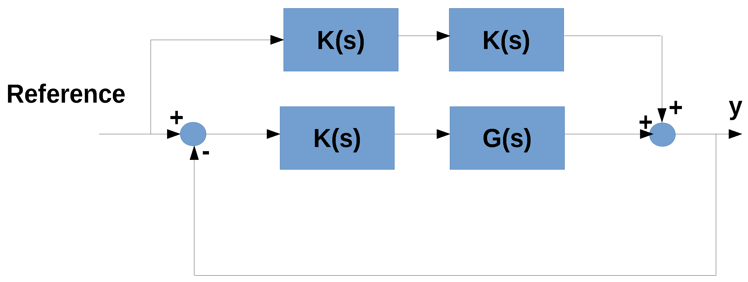
In this paper, the design of weighting filters based on elliptic functions is proposed. As explained in the previous section, elliptic functions provide a useful theoretical background to select functions with prescribed zeros and poles. Considering the double-periodicity of elliptic functions. The selection of the cross-over frequencies for the gain and phase margins, respectively, along with an appropriate cut-off frequency is straightforward. For this reason, the weighting filter design is done in a theoretical and accurate way, and it is not necessary to implement other design methodologies that are not stronger from a theoretical point of view. In this section, the design of a standard H-infinity loop shaping controller synthesis is shown. In Figure 1 the block diagram of the compensated closed-loop system is depicted, where is the controller obtained by loop shaping and is the plant.
3.1. Loop Shaping Design Procedure
The H-infinity loop shaping design procedure is done in the following steps [15]:
- Find the robust controller in order that the following condition is met:where is the complementary sensitivity closed-loop transfer function and and are given due to the following robust condition explained later:where and are the coprime factors withwhere and are the coprime factor uncertainties. Finally,It is important to consider that the gain shown in the feedforward compensated block diagram, depicted in Figure 1, is found using the equivalent block diagram shown in this figure. This complementary sensitivity function is obtained to derive the gain matrix and, later, the gain is obtained with the loop shaping design procedure as shown in step 2 and 3. Remember that in the robust loop shaping design given in (7), (8), and (9), the and are found obtaining the coprime factorization of the plant to be shaped as presented in Figure 2 and Figure 3.One of the novel contributions of this work is that the gain is obtained from the complementary function from Figure 1 to improve the robustness of the closed-loop system surpassing non compensated approaches as shown in [16]. As a conclusion of this robust loop shaping design procedure, first the gain matrix is obtained from the sensitivity function obtained from Figure 1 (feedforward compensated system) but considering the values of and obtained from (7)–(9) and the uncertainties of the diagrams shown in Figure 2 and Figure 3. Then, the loop shaping design procedure is concluded in steps 2 and 3.
- The second step is to find the weighting functions and in order to obtain a desired open-loop frequency response characteristic for in the following form . This step is crucial in this study because the weighting function selections are done by complex elliptic functions, for the standard and PID controller design.
- Finally, the controller is given by .
3.2. Weighting Function and Standard Controller Design with Complex Elliptic Functions
As explained before, one of the main issues that must be solved in the H-infinity loop shaping controller design is the selection of the weighting function. In this paper, a weighting function design implementing elliptic complex functions is proposed. Due to the double periodicity of elliptic functions the selection of an elliptic function with prescribed poles and zero is done, as explained in Section 2, to select the gain margin and phase margin along with the cut-off frequencies (step 2). Another improvement in comparison with other results is found in the literature that the controller is obtained to meet the robustness specifications.
In the following theorem, both issues explained in the previous paragraph are established [22].
Theorem 2.
The weighting functions and is obtained by using Abel’s theorem and the function explained later
in order to find the controller
Proof.
Define the following set:
The variable and the following function which is defined in Abel’s theorem to obtain an elliptic function with prescribed poles and zeros
where . Consider the following plant transfer function:
and the following complementary sensitivity function:
Then, according to the step 1 of the H-infinity loop shaping design the following result is obtained:
So by defining the transfer function:
the supremum of the sensitivity function shown in (15) is found as
To simplify the controller design it is necessary to implement a Taylor series expansion of the following function:
so
To derive the weighting filters, consider (12) with the frequencies and where T is the period. The weighting function which is a low pass filter is given by:
where
now, consider
Therefore, for and
and for and
Therefore, to avoid the exponential term, is approximated by a Taylor series-defining
Then, implementing only the first terms of the Taylor series expansion of
We obtain
and to define the numerator and denominator in (20), it is necessary to apply the following change of variables: and . The equivalent filter is given by:
and this completes the proof. □
To find the periods of the elliptic functions (, ) along with the crossover frequencies and cut-off frequencies (,,), the following equations must be solved by a nonlinear algebraic equation solver
where is the gain margin and is the required phase margin.
4. PID Loop Shaping Controller Synthesis by Elliptic Functions
Proportional-integral-derivative (PID) controllers were implemented in the process control and other applications [31,32,33,34,35]. For these reasons, as explained in the previous section, the H-infinity PID loop shaping controller system, given in Figure 4, is obtained by elliptic functions. The following theorem establishes the theoretical background for this objective.
Theorem 3.
The proportional-integral-derivative loop shaping controller synthesis is obtained by an unique weighting filter.
where is the proportional gain, is the derivative time constant and is the integral time constant.
Proof.
The PID controller is given by
Using the filter the following equivalent transfer function is obtained:
To find the elliptic function periods and along with the cross over frequencies , and the cutoff frequency , the following nonlinear algebraic equations must be solved numerically:
where is the gain margin and is the required phase margin.
5. Numerical Experiments
In this section, three numerical experiments are shown to test the theoretical results obtained in this study. The first and second experiments are developed considering a step and impulse response respectively, while the third numerical experiment is done by regulating the acid concentration in a water reservoir. The simulation is performed with GNU Octave 4.2.2 in an Intel Core i3 laptop. The plant used in the first and second experiment is:
5.1. Experiment 1
In experiment 1, the H-infinity loop shaping controller synthesis is tested in the control of system (36). The frequencies found for the weighting filters are rad/s and rad/s for and rad. Then, the following system response is found comparing the results with the strategies evinced in [36,37] as depicted in Figure 5.
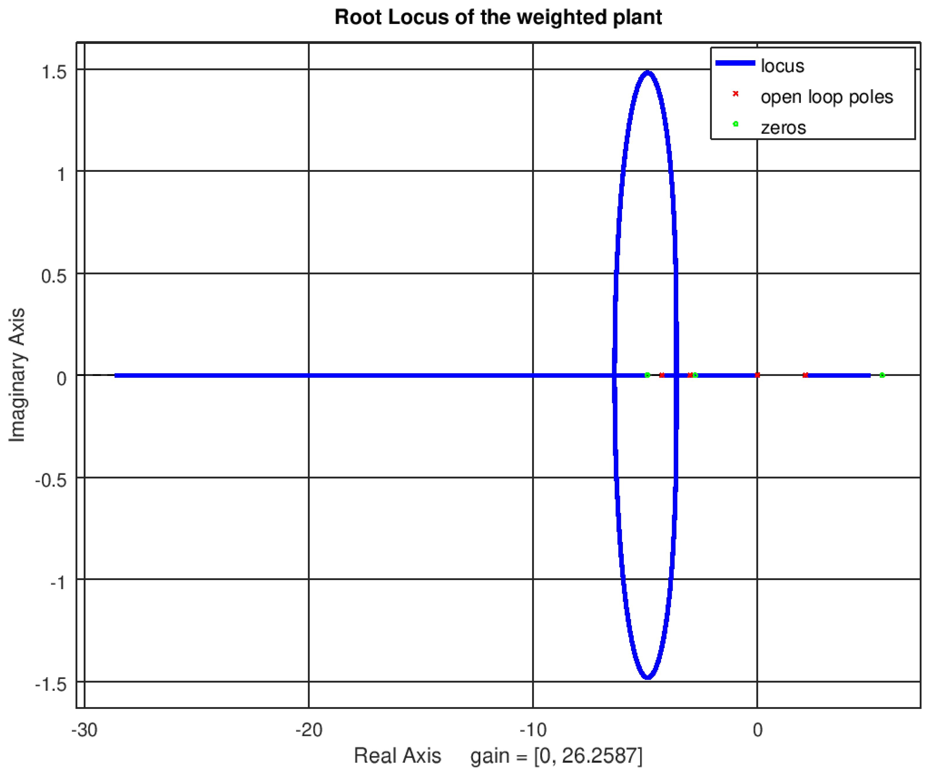
The system is tested with a step reference and an impulse reference, as can be noticed there, is less overshoot with the proposed approach in comparison with the approaches shown in [36,37] moreover, the steady-state error is smaller with the proposed strategy in comparison with the compared strategies. Then, in Figure 6 the error variable for both strategies is shown. As can be noticed the error between the reference and the output of the system is smaller with the proposed control strategy in comparison with the strategies shown in [36,37] proving the effectiveness of the controller design. In Figure 7 the root locus of the weighted and shaped plant is shown in which, as can be noticed, the addition of poles and/or zeros by the weighting filters shape the plant so that the system performance is improved by moving the locus region to the desired position. Then in Figure 8, the impulse response of the system is shown corroborating that the response reaches the zero value in a short time in opposition to the impulse response obtained with the approaches shown in [36,37].
The robustness index is given by the following:
Table 1 shows the robustness indexes of the three strategies. As can be noticed, the robustness index of the proposed strategy is smaller than [37] and greater than [36], this means that the proposed control strategy provides a moderate robustness index taking into consideration that there is a trade-off between the system performance index and robustness.
As can be noticed in Table 2 that when the integral squared error ISE increase, the robustness index decrease, or in other words they are inversely proportional, remarking again that our proposed method provides a moderated robustness index and performance in comparison with the other two comparative strategies. For this reason, the proposed control strategy provides its optimal performance.
5.2. Experiment 2
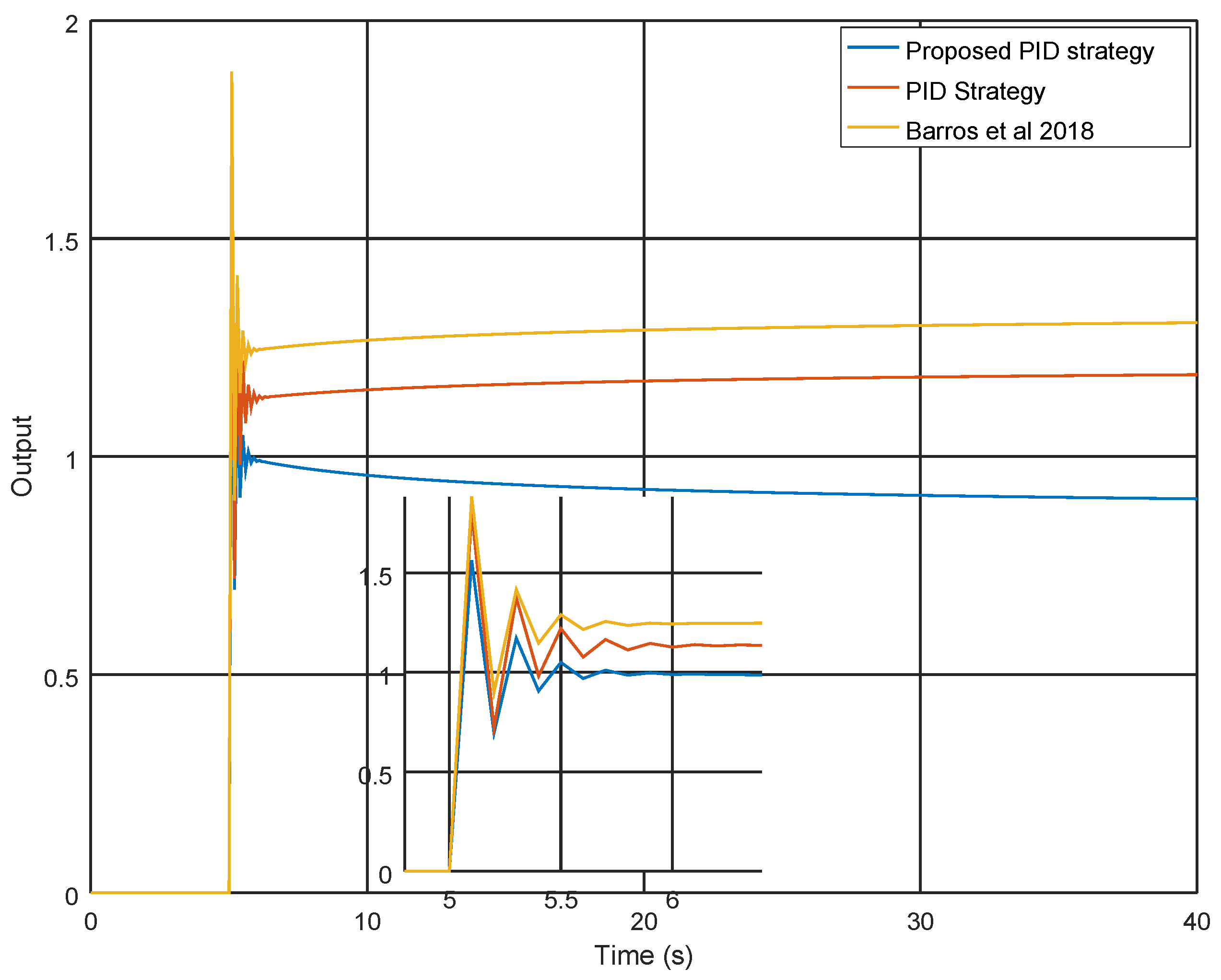
In this experiment, the loop shaping PID controller synthesis design is tested to corroborate the theoretical results obtained. The frequencies of the weighting functions are rad/s and rad/s with and rad.
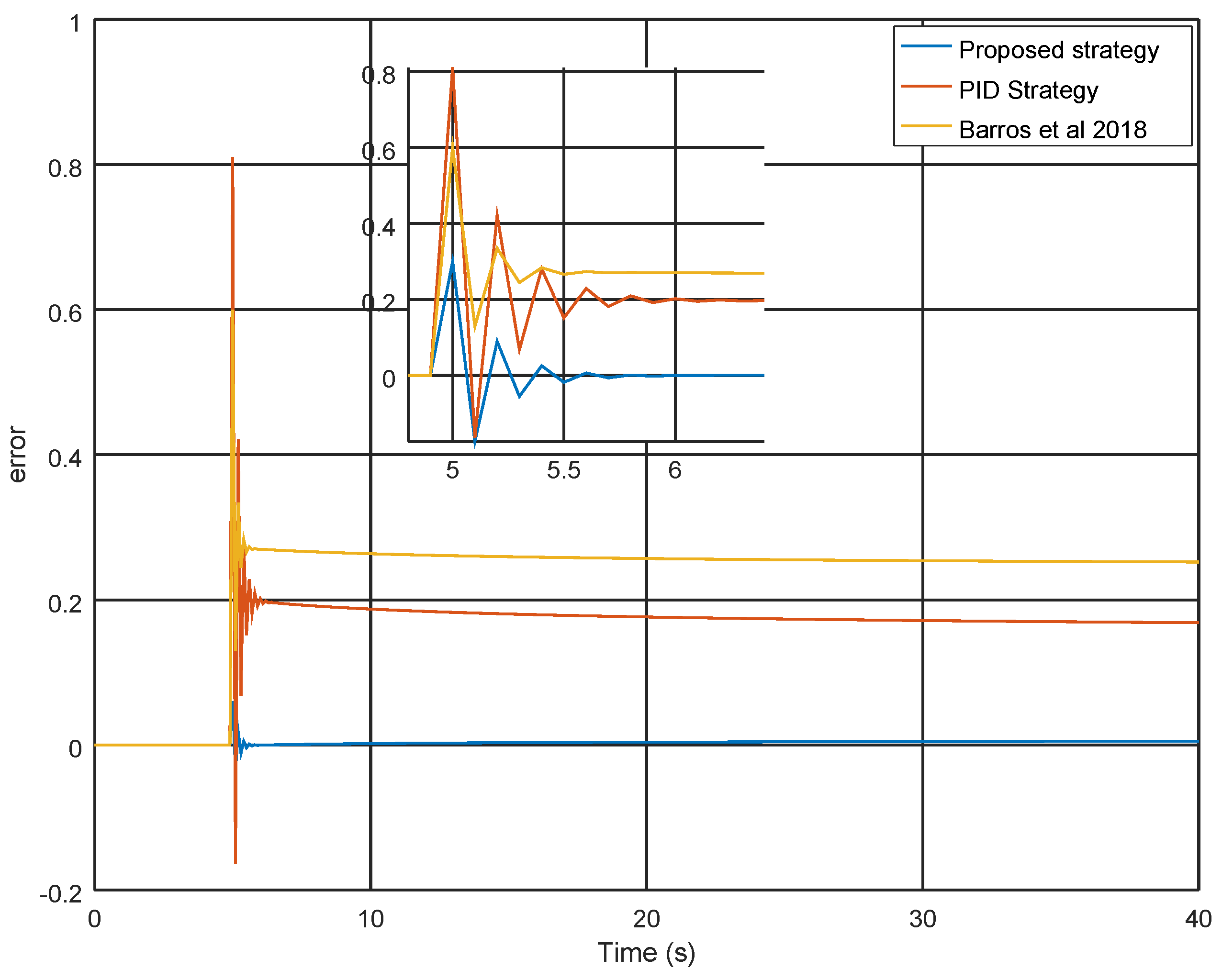
In Figure 9, the system response of the proposed strategy in comparison with the standard PID controller and the approaches shown in [38,39] are depicted. The overshoot and steady-state error are smallest than the standard PID controller so the H-infinity PID controller synthesis yields better results. In Figure 10 the error variable between the reference and the system output is presented and the steady-state error with the proposed controller synthesis is significantly smaller in comparison with the results obtained by [38,39].
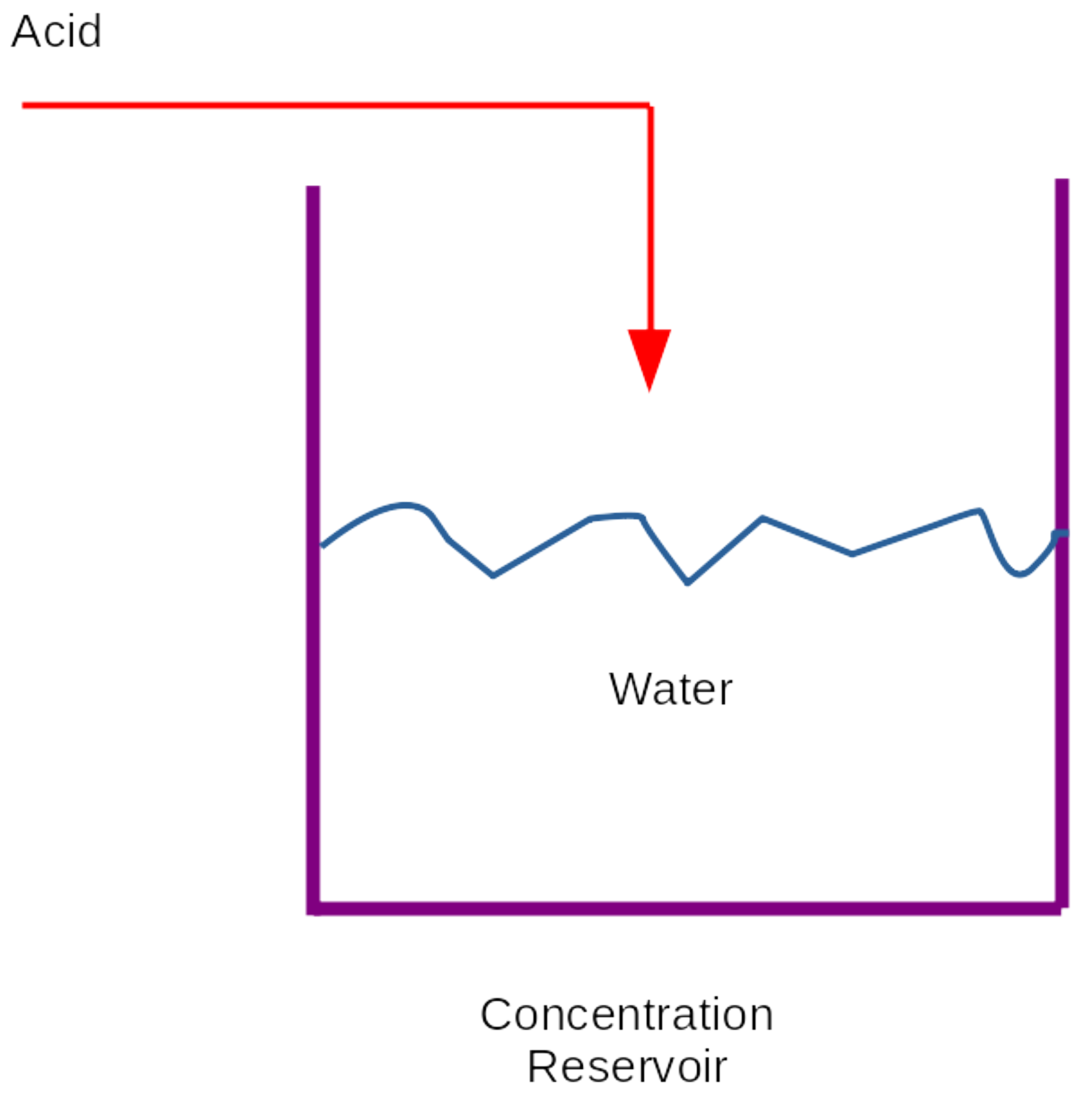
5.3. Experiment 3: Acid Concentration Regulation in a Water Reservoir
For this numerical experiment, consider the following mathematical model of a water reservoir with an acid input flow as appears in Figure 11. The mathematic model of the proposed system is [40]:
where V is the volume of the reservoir, C is the acid concentration in , U is the acid rate input and q is an appropriate constant. Then the transfer function is:
This numerical experiment consists of regulating the acid concentration in the water reservoir as 500 mol/m3 starting from a 0 mol/m3 concentration until the desired setpoint is reached.
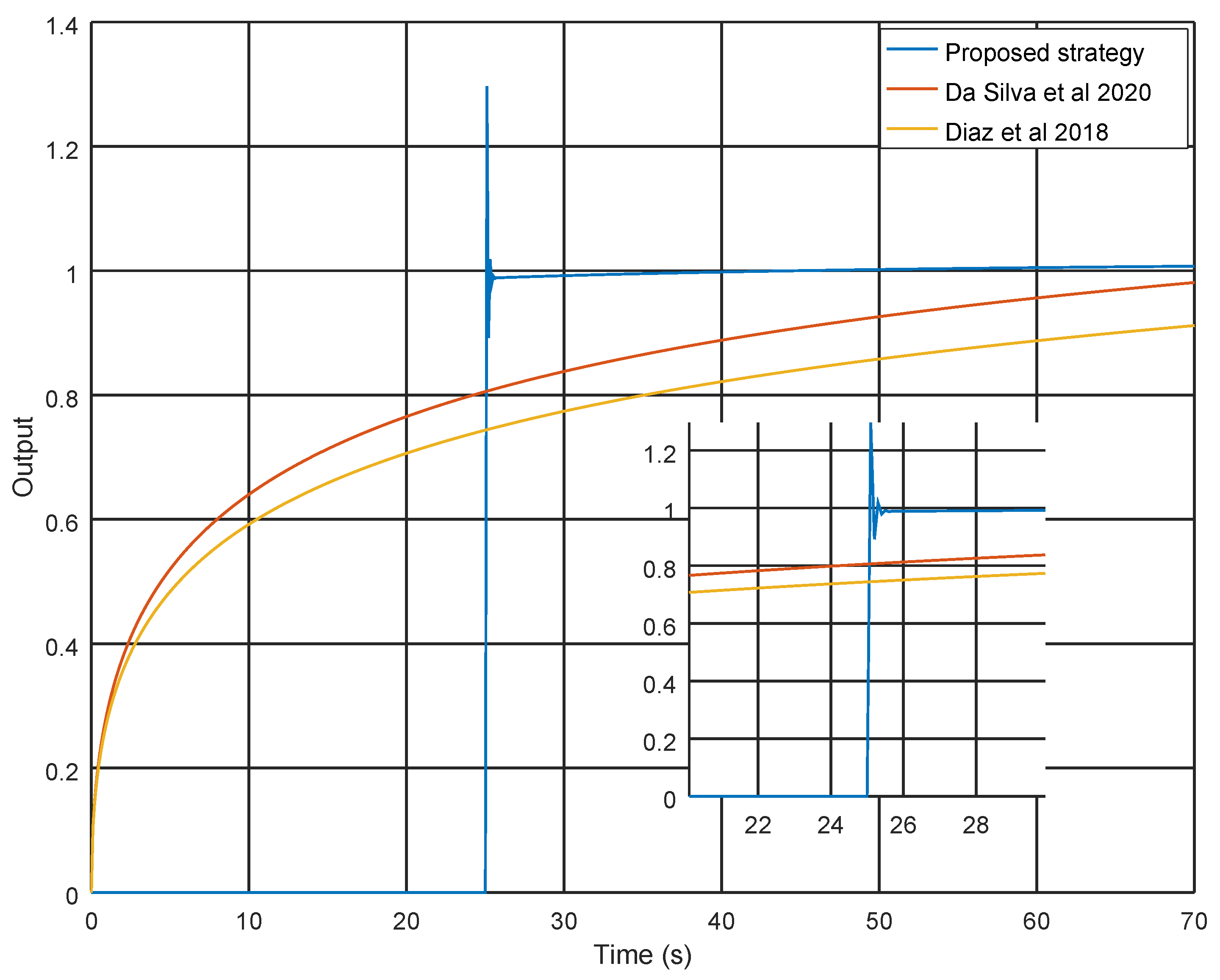
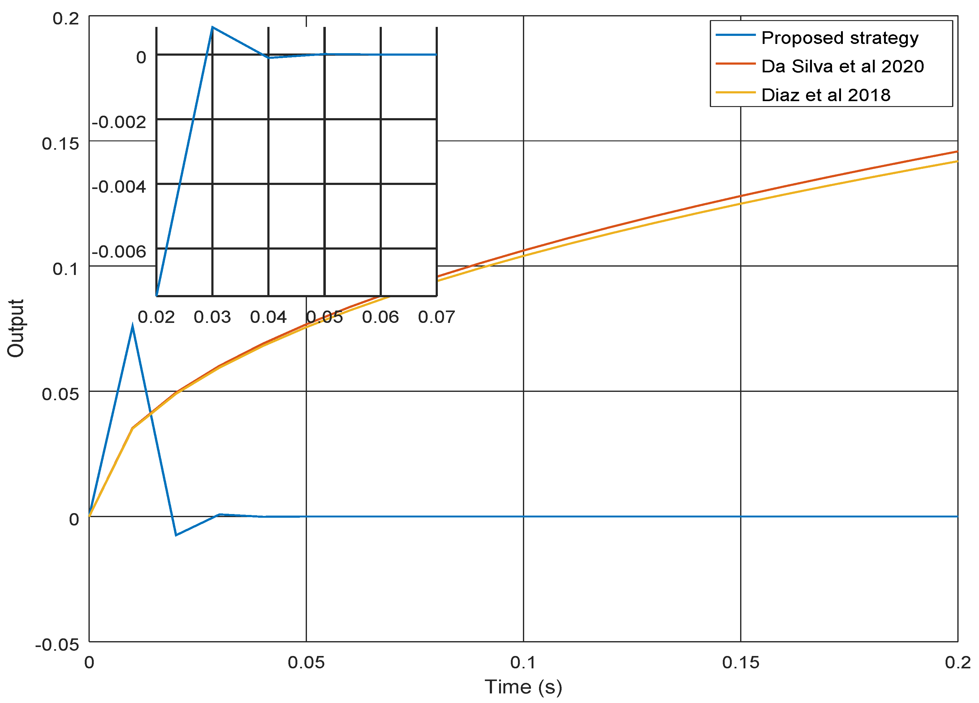
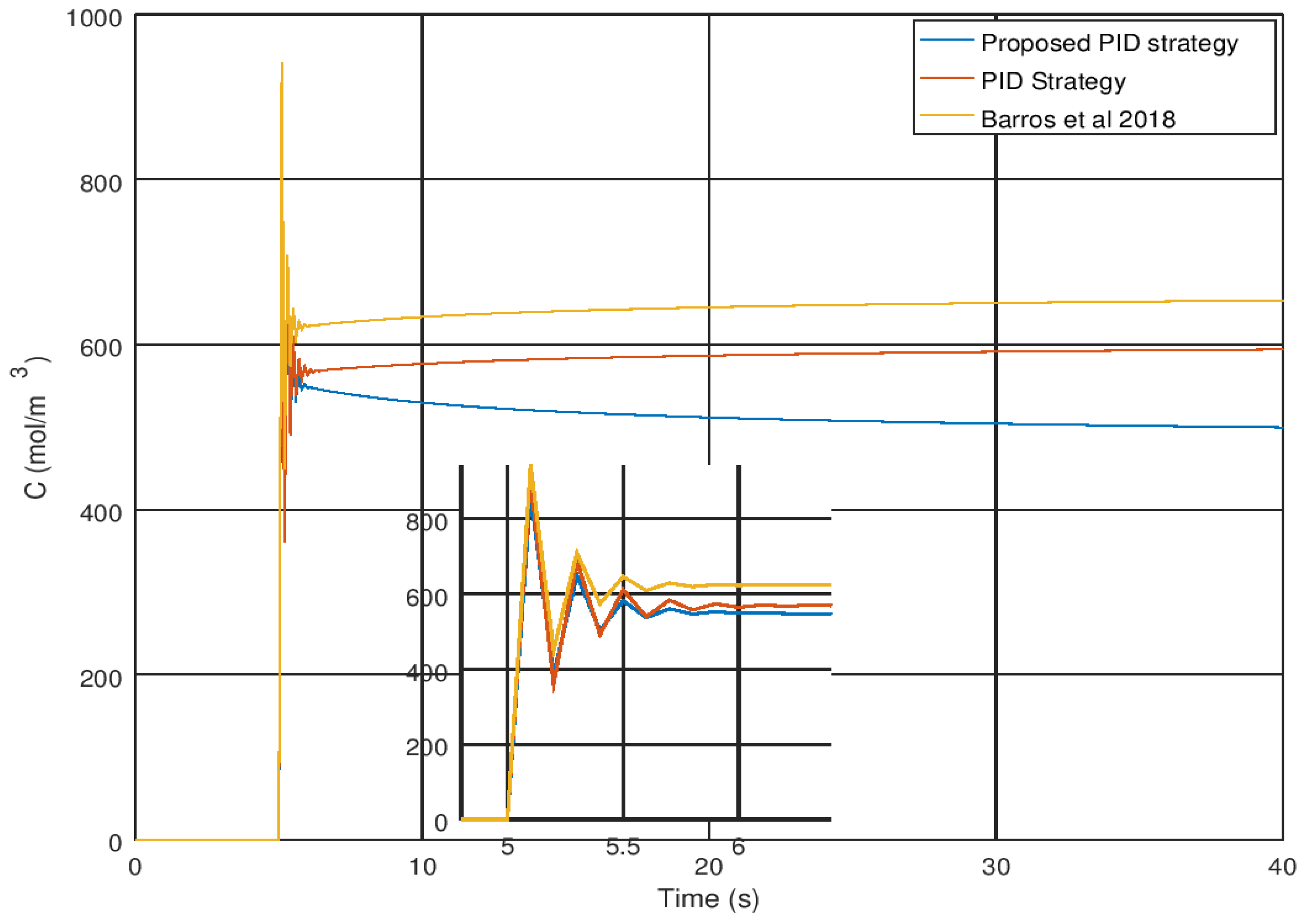
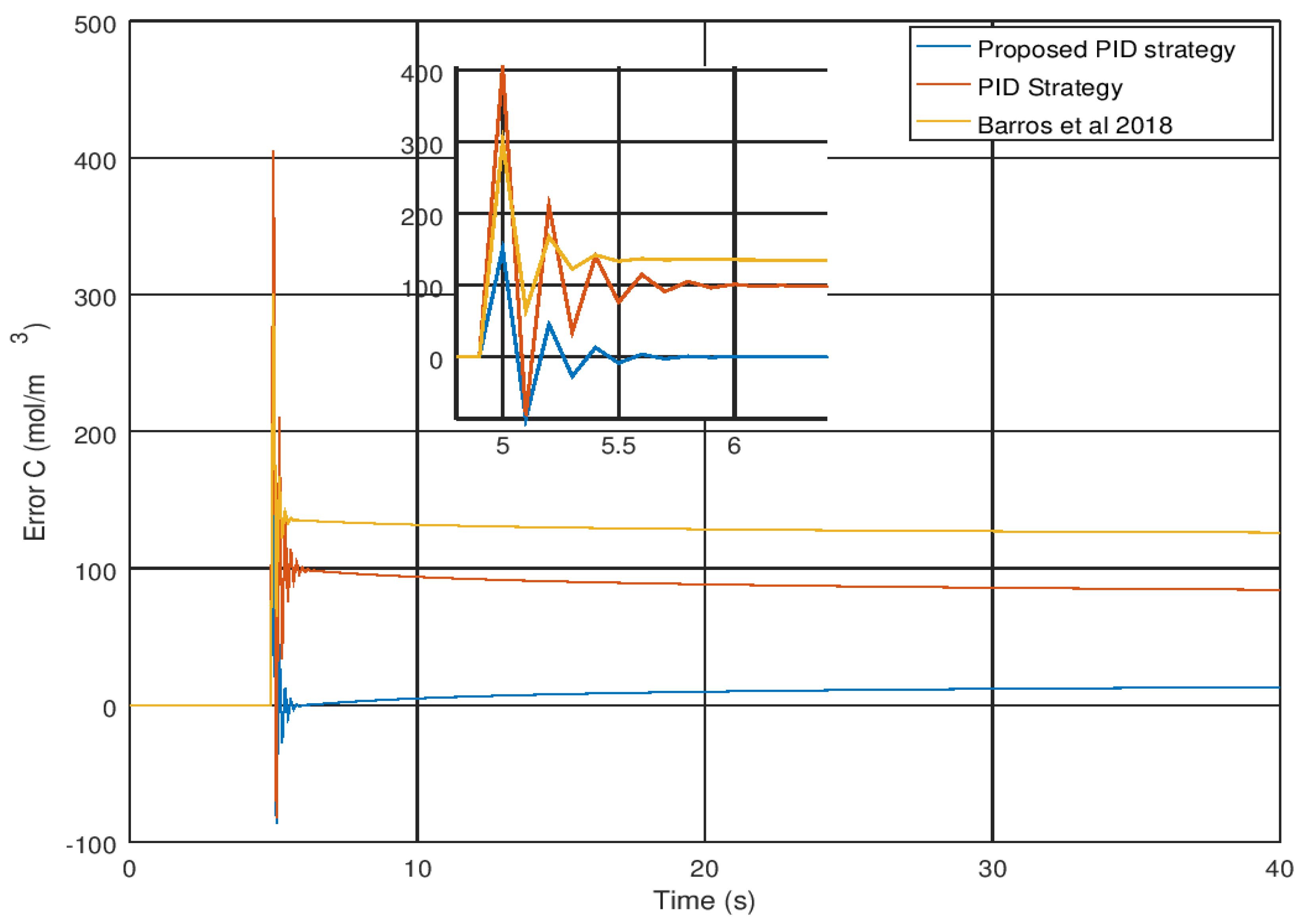
In Figure 12 and Figure 13, it can be noticed how the acid concentration reach the desired setpoint value when a step response is needed. It can be noticed how the acid concentration reaches the desired value faster, and as noticed in Figure 12, there is a fast change from the initial to the final desired setpoint value. It is important to observe that the results obtained with the proposed control strategy provide faster and more accurate results than the strategies proposed in [36,37]. These results are corroborated in Figure 13 in which it is noticed how a faster and smaller output response is obtained with the proposed control strategy in comparison with [36,37] something that proves that the proposed control strategy improves other results found in the literature.
6. Conclusions
In this article, a novel approach for the H-infinity loop shaping controller synthesis is proposed. Two of the main contributions shown in this article are the robust H-infinity controller derivation and the weighting function synthesis implementing the elliptic function to select the appropriate poles and zeros to meet the gain margin, phase margin, and cutoff frequency. It is proved, theoretically, that one of the main advantages of this approach is that there is a strong mathematical methodology to obtain the weighting filters and the gain matrices. Finally, these results were proved by numerical examples.
Author Contributions
Conceptualization, A.T.A. and F.E.S.; Formal analysis, A.T.A., F.E.S., N.A.K.; Methodology, A.T.A., F.E.S. and N.A.K.; Resources, F.E.S. and N.A.K.; Software, F.E.S. and N.A.K.; Supervision, A.T.A. Investigation A.T.A.; Validation A.T.A. and N.A.K.; Visualization, F.E.S. and N.A.K.; Writing—original draft, A.T.A., F.E.S. and N.A.K.; Writing—review & editing, A.T.A., F.E.S., N.A.K. All authors have read and agreed to the published version of the manuscript.
Funding
This research is funded by Prince Sultan University, Riyadh, Kingdom of Saudi Arabia. Special acknowledgement to Robotics and Internet-of-Things Lab (RIOTU), Prince Sultan University, Riyadh, Saudi Arabia. We would like to show our gratitude to Prince Sultan University, Riyadh, Saudi Arabia.
Conflicts of Interest
The authors declare no conflict of interest.
References
- Kim, S.M.; Pereira, J.; Lopes, V.; Turra, A.; Brennan, M. Practical active control of cavity noise using loop shaping: Two case studies. Appl. Acoust. 2017, 121, 65–73. [Google Scholar] [CrossRef] [Green Version]
- Pérez, J.; Cobreces, S.; Grino, R.; Sánchez, F. H-infinity current controller for input admittance shaping of VSC-based grid applications. IEEE Trans. Power Electron. 2017, 32, 3180–3191. [Google Scholar] [CrossRef] [Green Version]
- Mercader, P.; Astrom, K.; Banos, A.; Hagglund, T. Robust PID design based on QFT and convex-concave optimization. IEEE Trans. Control. Syst. Technol. 2017, 25, 441–452. [Google Scholar] [CrossRef]
- Usami, T.; Yubai, K.; Yashiro, D.; Komada, S. Multivariable fixed-structural controller design for H-infinity loop shaping method by iterative LMI optimization using frequency response data. In Proceedings of the International Conference on Advanced Mechatronic Systems, ICAMechS, Melbourne, Australia, 30 November–3 December 2017; pp. 218–223. [Google Scholar]
- Azar, A.T.; Serrano, F.E. Stabilization of Mechanical Systems with Backlash by PI Loop Shaping. Int. J. Syst. Dyn. Appl. 2016, 5, 21–46. [Google Scholar] [CrossRef] [Green Version]
- Azar, A.T.; Serrano, F.E.; Vaidyanathan, S. Proportional Integral Loop Shaping Control Design with Particle Swarm Optimization Tuning. In Advances in System Dynamics and Control; Azar, A.T., Vaidyanathan, S., Eds.; Advances in Systems Analysis, Software Engineering, and High Performance Computing (ASASEHPC); IGI Global: Hershey, PA, USA, 2018; pp. 24–57. [Google Scholar]
- Azar, A.T.; Serrano, F.E.; Kamal, N.A.; Koubaa, A. Robust Kinematic Control of Unmanned Aerial Vehicles with Non-holonomic Constraints. In Proceedings of the International Conference on Advanced Intelligent Systems and Informatics 2020, Cairo, Egypt, 19 October 2020; Hassanien, A.E., Slowik, A., Snášel, V., El-Deeb, H., Tolba, F.M., Eds.; Springer International Publishing: Cham, Switzerland, 2021; pp. 839–850. [Google Scholar]
- Meghni, B.; Dib, D.; Azar, A.T.; Ghoudelbourk, S.; Saadoun, A. Robust Adaptive Supervisory Fractional Order Controller for Optimal Energy Management in Wind Turbine with Battery Storage. In Fractional Order Control and Synchronization of Chaotic Systems; Studies in Computational Intelligence; Azar, A.T., Vaidyanathan, S., Ouannas, A., Eds.; Springer International Publishing: Cham, Switzerland, 2017; Volume 688, pp. 165–202. [Google Scholar]
- Pereira, R.L.; Kienitz, K.H. H-infinity Loop Shaping Control of Input Saturated Systems with Norm Bounded Parametric Uncertainty. J. Control. Sci. Eng. 2015, 2015, 383297. [Google Scholar] [CrossRef] [Green Version]
- Zhou, S.L.; Han, P.; Wang, D.F.; Liu, Y.Y. A kind of multivariable PID design method for chaos system using H-infinity loop shaping design procedure. In Proceedings of the 2004 International Conference on Machine Learning and Cybernetics, Shanghai, China, 26–29 August 2004. [Google Scholar]
- Kojima, A.; Ichikawa, Y. H-infinity loop-shaping procedure for multiple input delay systems. In Proceedings of the 46th IEEE Conference on Decision and Control, New Orleans, LA, USA, 12–14 December 2007. [Google Scholar]
- Ouddah, N.; Boukhnifer, M.; Chaibet, A.; Monmasson, E. Fixed structure H-infinity loop shaping control of switched reluctance motor for electrical vehicle. Math. Comput. Simul. 2016, 130, 124–141. [Google Scholar] [CrossRef]
- Iqbal, S.; Bhatti, A.I.; Akhtar, M.; Ullah, S. Design and robustness evaluation of an H-infinity loop shaping controller for a 2DOF stabilized platform. In Proceedings of the 2007 European Control Conference (ECC), Kos, Greece, 2–5 July 2007. [Google Scholar]
- Boeren, F.; van Herpen, R.; Oomen, T.; van de Wal, M.; Bosgra, O. Enhancing performance through multivariable weighting function design in H-infinity loop-shaping with application to a motion system. In Proceedings of the 2013 American Control Conference, Washington, DC, USA, 17–19 June 2013. [Google Scholar]
- Phurahong, N.; Kaitwanidvilai, S.; Ngaopitakkul, A. Fixed Structure Robust 2DOF H-infinity Loop Shaping Control for ACMC Buck Converter using Genetic Algorithm. In Proceedings of the International Multiconference of Engineers and Computer Scientist 2012, Hong Kong, China, 14–16 March 2012. [Google Scholar]
- Boukhnifer, M.; Ferreira, A. H-infinity Loop Shaping for Stabilization and Robustness of a Tele-Micromanipulation System. In Proceedings of the IEEE/RSJ International Conference on Intelligent Robots and Systems, Edmonton, AB, Canada, 2–6 August 2005. [Google Scholar]
- Osinuga, M.; Patra, S.; Lanzon, A. Weight optimization for maximizing robust performance in H-infinity loop-shaping design. IFAC Proc. Vol. 2011, 44, 10135–10140. [Google Scholar] [CrossRef]
- Formentin, S.; Karimi, A.; Savaresi, S.M. Direct data-driven H2-H-infinity loop-shaping. IFAC Proc. Vol. 2011, 44, 11423–11428. [Google Scholar] [CrossRef] [Green Version]
- Prempain, E. Gain-Scheduling H-infinity Loop Shaping Control Of Linear Parameter-Varying Systems. IFAC Proc. Vol. 2006, 39, 215–219. [Google Scholar] [CrossRef]
- Lee, C.F.; Khong, S.Z.; Frisk, E.; Krysander, M. An extremum seeking approach to parameterised loop-shaping control design. IFAC Proc. Vol. 2014, 47, 10251–10256. [Google Scholar] [CrossRef]
- Suh, B.; Yun, S.; Yang, J. A New Loop-Shaping Procedure for Tuning LQ-PID Regulator. IFAC Proc. Vol. 2003, 36, 271–276. [Google Scholar] [CrossRef]
- Freitag, E.; Busam, R. Complex Analysis; Springer: Berlin/Heidelberg, Germany, 2009. [Google Scholar]
- Iapichino, L.; Quarteroni, A.; Rozza, G. Reduced basis method and domain decomposition for elliptic problems in networks and complex parametrized geometries. Comput. Math. Appl. 2016, 71, 408–430. [Google Scholar] [CrossRef]
- Siegl, P.; Štampach, F. On extremal properties of Jacobian elliptic functions with complex modulus. J. Math. Anal. Appl. 2016, 442, 627–641. [Google Scholar] [CrossRef] [Green Version]
- Azar, A.T.; Serrano, F.E. Robust IMC–PID tuning for cascade control systems with gain and phase margin specifications. Neural Comput. Appl. 2014, 25, 983–995. [Google Scholar] [CrossRef]
- Armana, C.; Wei, F.T. Sturm-type bounds for modular forms over function fields. J. Number Theory 2020. [Google Scholar] [CrossRef]
- Choie, Y. Periods of Hilbert modular forms, Kronecker series and cohomology. Adv. Math. 2021, 381, 107617. [Google Scholar] [CrossRef]
- Wang, G.; Zhang, X.; Chu, Y. Inequalities for the generalized elliptic integrals and modular functions. J. Math. Anal. Appl. 2007, 331, 1275–1283. [Google Scholar] [CrossRef] [Green Version]
- Virdol, C. Potential modularity for elliptic curves and some applications. J. Number Theory 2009, 129, 3109–3114. [Google Scholar] [CrossRef] [Green Version]
- Winding, J. Multiple elliptic gamma functions associated to cones. Adv. Math. 2018, 325, 56–86. [Google Scholar] [CrossRef] [Green Version]
- Ibraheem, G.A.R.; Azar, A.T.; Ibraheem, I.K.; Humaidi, A.J. A Novel Design of a Neural Network-Based Fractional PID Controller for Mobile Robots Using Hybridized Fruit Fly and Particle Swarm Optimization. Complexity 2020, 2020, 1–18. [Google Scholar] [CrossRef]
- Pilla, R.; Botcha, N.; Gorripotu, T.S.; Azar, A.T. Fuzzy PID Controller for Automatic Generation Control of Interconnected Power System Tuned by Glow-Worm Swarm Optimization. In Applications of Robotics in Industry Using Advanced Mechanisms; Nayak, J., Balas, V.E., Favorskaya, M.N., Choudhury, B.B., Rao, S.K.M., Naik, B., Eds.; Springer International Publishing: Cham, Switzerland, 2020; pp. 140–149. [Google Scholar]
- Soliman, M.; Azar, A.T.; Saleh, M.A.; Ammar, H.H. Path Planning Control for 3-Omni Fighting Robot Using PID and Fuzzy Logic Controller. In Proceedings of the International Conference on Advanced Machine Learning Technologies and Applications (AMLTA2019), Jaipur, India, 13–15 February 2020; pp. 442–452. [Google Scholar]
- Ammar, H.H.; Azar, A.T. Robust Path Tracking of Mobile Robot Using Fractional Order PID Controller. In Proceedings of the International Conference on Advanced Machine Learning Technologies and Applications (AMLTA2019), Jaipur, India, 13–15 February 2020; Volume 921, pp. 370–381. [Google Scholar]
- Sallam, O.K.; Azar, A.T.; Guaily, A.; Ammar, H.H. Tuning of PID Controller Using Particle Swarm Optimization for Cross Flow Heat Exchanger Based on CFD System Identification. In Proceedings of the International Conference on Advanced Intelligent Systems and Informatics 2019, Cairo, Egypt, 19–21 October 2020; Volume 1058, pp. 300–312. [Google Scholar]
- Díaz, J.M.; Dormido, S.; Costa-Castelló, R. The use of interactivity in the controller design: Loop shaping versus closed-loop shaping. IFAC-PapersOnLine 2018, 51, 334–339. [Google Scholar] [CrossRef]
- da Silva, L.R.; Flesch, R.C.C.; Normey-Rico, J.E. Controlling industrial dead-time systems: When to use a PID or an advanced controller. ISA Trans. 2020, 99, 339–350. [Google Scholar] [CrossRef] [PubMed]
- Anwar, M.N.; Pan, S. Synthesis of the PID controller using desired closed-loop response. IFAC Proc. Vol. 2013, 46, 385–390. [Google Scholar] [CrossRef] [Green Version]
- Barros, C.P.B.; Barros, P.R.; da Rocha Neto, J.S. Loop Shaping for PID Controller Design Based on Time and Frequency Specifications. IFAC-PapersOnLine 2018, 51, 592–597. [Google Scholar]
- Skogestad, S. A procedure for siso controllability analysis: With application to design of pH processes. In Integration of Process Design and Control; Zafiriou, E., Ed.; Pergamon: Oxford, UK, 1994; pp. 25–30. [Google Scholar]
Figure 1.
Block diagram of the compensated closed-loop system.

Figure 2.
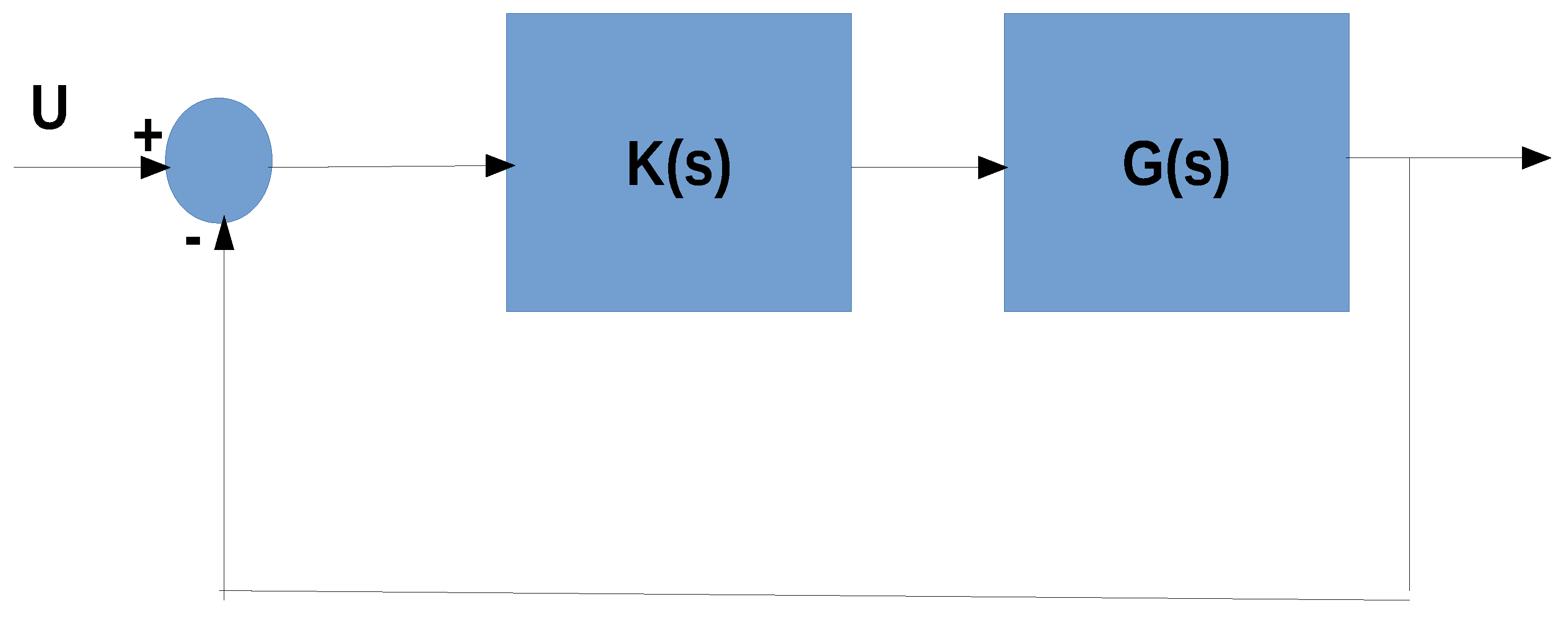
Block diagram for the loop shaping design.

Figure 3.
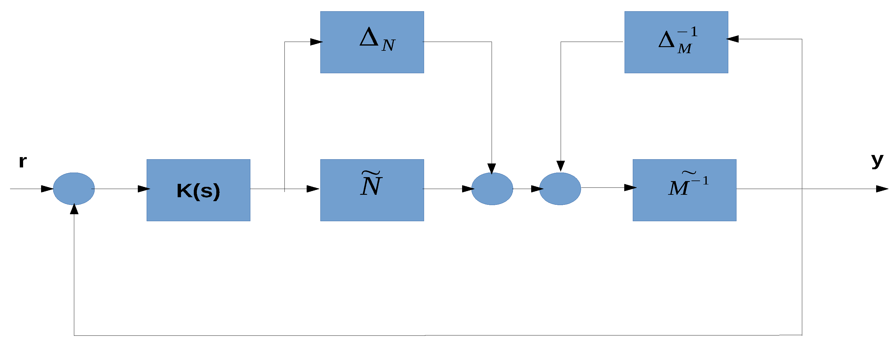
Coprime factor robust stabilization.

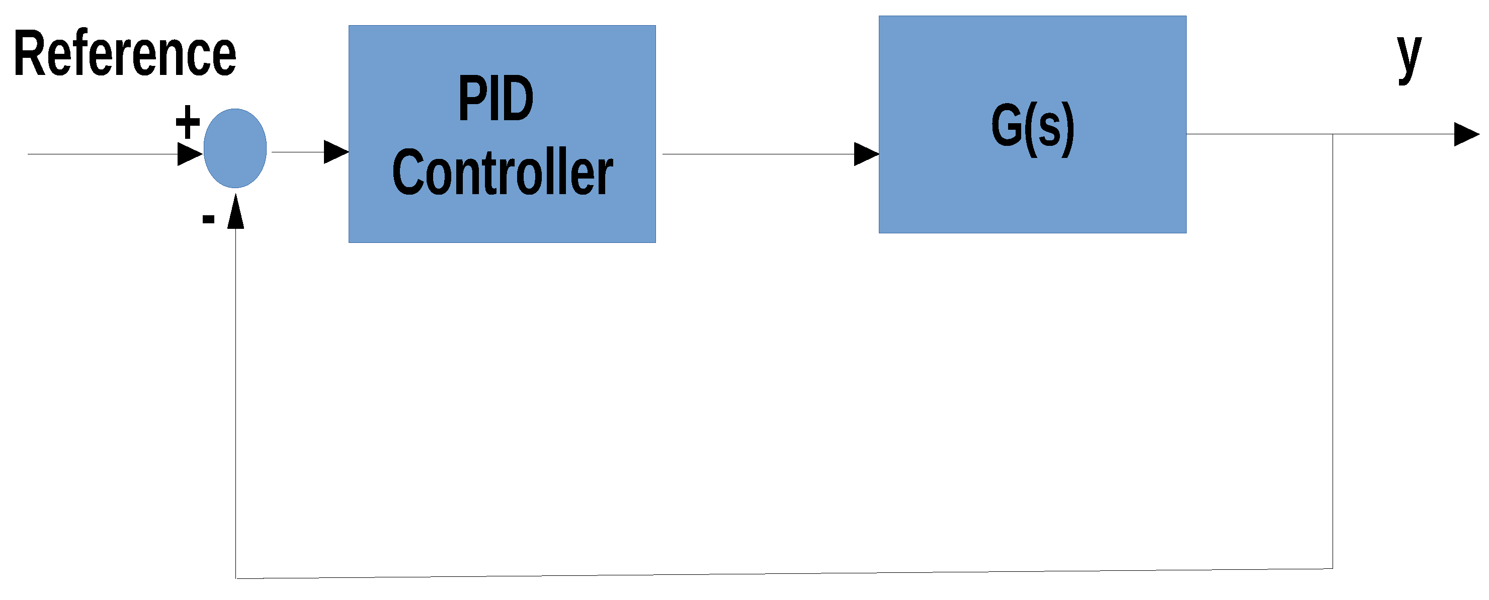
Figure 4.
Closed loop system block diagram.

Figure 5.
System response.

Figure 6.
Error Variable for Experiment 1.

Figure 7.
Root locus of the weighted plant for the analyzed system.

Figure 8.
Impulse response.

Figure 9.
System response.

Figure 10.
Error Variable for Experiment 2.

Figure 11.
Schematic diagram of the water reservoir considered in this experiment.

Figure 12.
Concentration level in the water reservoir.

Figure 13.
Concentration error in the water reservoir.


Publisher’s Note: MDPI stays neutral with regard to jurisdictional claims in published maps and institutional affiliations. |
© 2021 by the authors. Licensee MDPI, Basel, Switzerland. This article is an open access article distributed under the terms and conditions of the Creative Commons Attribution (CC BY) license (http://creativecommons.org/licenses/by/4.0/).
Share and Cite
MDPI and ACS Style
Azar, A.T.; Serrano, F.E.; Kamal, N.A. Robust H∞ Loop Shaping Controller Synthesis for SISO Systems by Complex Modular Functions. Math. Comput. Appl. 2021, 26, 21. https://0-doi-org.brum.beds.ac.uk/10.3390/mca26010021
AMA Style
Azar AT, Serrano FE, Kamal NA. Robust H∞ Loop Shaping Controller Synthesis for SISO Systems by Complex Modular Functions. Mathematical and Computational Applications. 2021; 26(1):21. https://0-doi-org.brum.beds.ac.uk/10.3390/mca26010021
Chicago/Turabian StyleAzar, Ahmad Taher, Fernando E. Serrano, and Nashwa Ahmad Kamal. 2021. "Robust H∞ Loop Shaping Controller Synthesis for SISO Systems by Complex Modular Functions" Mathematical and Computational Applications 26, no. 1: 21. https://0-doi-org.brum.beds.ac.uk/10.3390/mca26010021