Modeling and Optimizing the Multi-Objective Portfolio Optimization Problem with Trapezoidal Fuzzy Parameters

Abstract

A common issue in the Multi-Objective Portfolio Optimization Problem (MOPOP) is the presence of uncertainty that affects individual decisions, e.g., variations on resources or benefits of projects. Fuzzy numbers are successful in dealing with imprecise numerical quantities, and they found numerous applications in optimization. However, so far, they have not been used to tackle uncertainty in MOPOP. Hence, this work proposes to tackle MOPOP’s uncertainty with a new optimization model based on fuzzy trapezoidal parameters. Additionally, it proposes three novel steady-state algorithms as the model’s solution process. One approach integrates the Fuzzy Adaptive Multi-objective Evolutionary (FAME) methodology; the other two apply the Non-Dominated Genetic Algorithm (NSGA-II) methodology. One steady-state algorithm uses the Spatial Spread Deviation as a density estimator to improve the Pareto fronts’ distribution. This research work’s final contribution is developing a new defuzzification mapping that allows measuring algorithms’ performance using widely known metrics. The results show a significant difference in performance favoring the proposed steady-state algorithm based on the FAME methodology.

1. Introduction

The Portfolio Optimization Problem (POP) is always present in organizations. One key issue in POP’s decision process is the uncertainty caused by the variability in the project benefits and resources. The latter situation arises the necessity of a tool for describing and representing uncertainty associated with real-life decision-making situations. The POP searches a subset of projects under a predefined set of resources that maximizes the produced benefits; its formal definition is as follows.

Let A be a finite set of N projects, each characterized by estimates of its impacts and resource consumption. A portfolio is a subset of A that can be represented by a binary vector $x=❬x_1, x_2, \dots ,x_n❭$ that assigns $x_i=1$ for every financed project i, and $x_i=0$ otherwise. Let $\overrightarrow{z} \left(x\right)=❬z_1 \left(x\right), z_2\left(x\right),\dots ,z_p\left(x\right)❭$ be the vector of impacts resulting from the linear sum of the attribute values of each financed project in x, i.e., the vector of size p representing multiple attributes related to organizational goals that describe the consequences of a portfolio $x$. Assume w.l.o.g. that the higher an attribute’s value is, the better. Then, Problem (1) formally defines POP.

$$Maximize\{❬z_1\left(x\right),z_2\left(x\right),\dots ,z_p\left(x\right)❭\}, x \in R_F$$

(1)

In Problem (1), R_F is the space of feasible portfolios, usually determined by the available budget and other constraints that the Decision Maker (DM) wants to impose (e.g., budget limits on types, geographic areas, social roles of projects, etc.).

Different scientific research works address POP’s variant in Problem (1), considering precise values on the available resources and the projects’ impacts [1,2,3,4,5,6]. Moreover, there is an area called Portfolio Decision Analysis (PDA) dedicated to studying mathematical models to solve POP. There are theories, methods, and practices developed within this area to help decision-makers select projects from a very large set of them, taking into account relevant constraints, preferences, uncertainty, or imprecision [7]. PDA-related problems’ difficulty comes from a combination of factors such as (1) large entry space; (2) consequences of multidimensionality in portfolio construction and selection; or (3) qualitative, imprecise or uncertain information.

A large entry space requires a solution process with exponential complexity for decision-making problems, even with simple decisions on allocating resources for candidate projects.

The consequences of multidimensionality in portfolio construction and selection relate conflicting attributes with difficulty in the decision process. Usually, the larger the number of dimensions, the more complex the solution space is. The latter causes a situation with so many solutions that it easily exceeds the human cognitive capabilities for evaluating and selecting the best candidate solutions [8].

The qualitative, imprecise, or uncertain information exists because of the varying nature of the distinct attributes and resources considered in the construction of portfolios. Such information can sometimes occur from different circumstances as a DM needs to use non-numerical data to describe the effects of a project instead of a quantitative measure. Other cases might indicate that there is lack of knowledge about future states of specific criteria, vagueness in the provided information, the values used to describe attributes or resources are not accurately known beforehand, or vague approximations and areas of ignorance. All the previous situations, denoted hereafter as uncertainty, limit the scientific approach in Operational Research-Decision Aiding [9], and modeling them using probability distributions can be a challenge [9].

Several optimization problems use fuzzy numbers to model the uncertainty in parameters’ values from arbitrariness, imprecision, and poor determination [10]. Among the most recent and works related to the Multi-objective Portfolio Optimization Problem are the following: García [11] solved the Multi-objective and Static Portfolio Optimization Problem (MOSPOP) with real parameters using the generational algorithms HHGA-SPPv1 and HHGA-SPPv2 and considering the preferences of a DM. Rivera-Zarate [12] uses the Non-Outranked Ant Colony Optimization (NO-ACO) to address a variant of MOSPOP that includes interdependency among objectives and that has partial support with real parameters. Bastiani [13] solves the MOSPOP variant that includes synergy using ACO-SPRI, ACO-SOP, and ACO-SOP, three strategies based on the ACO that incorporate in their search process priority ranking, preferences, and synergy, respectively. Sánchez [14] proposes using classification methods on the generational algorithms H-MCSGA and I-MCSGA to approximate the Region of Interest (ROI) in MOSPOP. The first algorithm adds the preferences at the beginning of the process, while the second algorithm adds them during the process (while interacting with the DM). Balderas addresses the MOSPOP with uncertainty using intervals; it proposes the generational algorithm I-NOSGA based on NSGAII but incorporates interval numbers. I-NOSGA includes preferences “a priori” and uses Crowding Distance as its density estimator. Martínez [15] addresses the Dynamic Multi-objective Portfolio Optimization Problem (DMOPOP) with real parameters; the proposed approach introduces dynamism by changing the problem definition at the end of each period. Martínez presents three new multi-objective algorithms that also incorporate “a priori” preferences: the generational D-NSGA-II-FF, a new version of a classic genetic algorithm of no-dominance; the D-AbYSS-FF, a modified version of scatter search; and the D-MOEA\D-FF, a new variant of a state-of-the-art algorithm based on decomposition.

Table 1. Related works.

Work	Algorithm	Instances	Metrics	Preferences	E/D	Parameters	Steady State
[11] Social projects	HHGA-SPPv1 HHGA-SPPv2	(3,4,20) (3,9,100)	No-dominated Solutions	Yes	E	Real	NA
[12] Interdependent social projects, several objectives	NO-ACO	(10,4,25) (10,9,100)	No-dominated Solutions, ROI solutions	Yes	E	Real	NA
[13] Social projects with priorities and sinergy	ACO-SPRI ACO-SOP ACO-SOP sinergy	(1,ND,25) (1,ND,40) (1,ND,100)	No-dominated Solutions	Yes	E	Real	NA
[14] Social projects, several objectives	H-MCSGA I-MCSGA	(3,9,100) (2,9,150) (1,16,500)	No-dominated solutions, higher net flow	Yes	E	Real	No
[10] Portfolio selection with interval parameters	I-NSGA-II-CD	(1,2,100) (1,9,100)	Cardinality	Yes	E	Intervals	No
[15] Dynamic portfolio selection and several objectives	D-NSGA-II-FF AbYSS-FF D-MOEA\D--FF	(30,2,100) (30,3,100) (30,9,100)	Hypervolume modified, Spread modified, inverted generational distance modified	Yes	D	Real	No
This work Portfolio selection with trapezoidal fuzzy numbers	T-NSGA-II-CD T-NSGA-II-SSD T-FAME	(12,2,25) (9,2,100)	Hypervolume, Generalized Spread	No	E	Trapezoidal fuzzy numbers	Yes

summarizes the main features of the previously described works. Column 1 cites the research work and the studied POP variant. Columns 2 to 7 show the considered features in the research works: the solution algorithms it proposed, the type of instances it solved, the performance metrics it used, if it integrated preferences in the search process, if it considered a static or dynamic POP’s version, the type of parameters it used, and if it used a steady-state selection scheme or not.

It is worth nothing that, from the information in Table 1, only approaches based on intervals address POP’s variant with uncertainty, and none of them utilized a steady-state selection scheme. The Fuzzy Adaptive Multi-objective Evolutionary solution methodology (FAME) has had great success in many optimization problems; however, there is a lack of studies about its performance on the POP. The previous situations open an area of opportunity, addressed in this work, consisting of studying optimization approaches’ performance derived from fuzzy numbers and steady-state selection schemes on their search process to solve the Multi-objective POP with uncertainty (MOPOP).

Evolutionary algorithms commonly use a generational selection scheme to update each generation’s population; the process creates several offspring through genetic operators and combines them with the parents to form the next generation of individuals [10,14,15]. On the other hand, an algorithm using a steaty-state selection scheme produces a single offspring during the reproduction process to combine with the parents. The efficiency of the population’s update process achieved by the latter method is advantageous for any research [16]. Hence, this work proposes a new method based on FAME and fuzzy numbers to handling uncertainty and obtaining more robust solutions in MOPOP; the approach mainly uses fuzzy trapezoidal sets to reflect a magnitude’s imprecision.

This work’s main contributions are: (1) a new mathematical model for MOPOP that considers fuzzy trapezoidal parameters; (2) a new algorithm based on FAME to solve the proposed model; (3) two novel steady-state NSGA-II to solve this MOPOP’s variant; and (4) a novel strategy to measure the performance of the fuzzy multi-objective algorithms with the commonly used real metrics.

The remaining structure of this paper is as follows. Section 2 includes some elements of the fuzzy theory used in this work. Section 3 describes a new mathematical model of the Portfolio Optimization Problem with Trapezoidal Fuzzy Parameters. Section 4 and Section 5 contain the proposed steady-state algorithms: T-NSGA-II and T-FAME, respectively. Section 6 describes the computational experiments done to assess the performance of the algorithms. Finally, Section 7 presents the conclusions.

2. Elements of Fuzzy Theory

This section contains the main concepts of fuzzy theory used in this work.

2.1. Fuzzy Sets

Let X be a collection of objects x, then a fuzzy set A defined over X is a set of ordered pairs A = {(x, μ_A(x))/x є X} where μ_A(x) is called the membership function or grade of membership of x in A which maps X to the real membership subspace M [17]. The range of the membership function is a subset of the nonnegative real numbers whose supremum is finite. Elements with a zero degree of membership usually are not listed.

2.2. Generalized Fuzzy Numbers

A generalized fuzzy number A is any fuzzy subset of the real line R, whose membership function ${\mathsf{\mu }}_{\mathrm{A}}\left(\mathrm{x}\right)$ satisfies the following conditions [18]:

• ${\mathsf{\mu }}_{\mathrm{A}}\left(\mathrm{x}\right)$ is a continuous function from $R$ to the closed interval $\left[0, 1\right]$
• ${\mathsf{\mu }}_{\mathrm{A}}\left(\mathrm{x}\right)=0,-\infty < \mathrm{x}< \mathrm{a}$
• ${\mathsf{\mu }}_{\mathrm{A}}\left(\mathrm{x}\right)=\mathrm{L}\left(\mathrm{x}\right)$, is strictly increasing on $\left[\mathrm{a}, \mathrm{b}\right]$
• ${\mathsf{\mu }}_{\mathrm{A}}\left(\mathrm{x}\right)= \mathrm{w}$, for $\mathrm{b}<\mathrm{x}<\mathsf{\alpha }$
• ${\mathsf{\mu }}_{\mathrm{A}}\left(\mathrm{x}\right)=\mathrm{R}\left(\mathrm{x}\right)$ is strictly decreasing on $\left[\mathsf{\alpha }, \mathsf{\beta }\right]$
• ${\mathsf{\mu }}_{\mathrm{A}}\left(\mathrm{x}\right)=0$, for $\mathsf{\beta }<\mathrm{x}<\infty$

where $0<w<1, a, b,\alpha ,\beta$ are real numbers.

We denote this type of generalized fuzzy number as $\mathrm{A}={\left(\mathrm{a},\mathrm{b},\mathsf{\alpha },\mathsf{\beta }, \mathrm{w}\right)}_{\mathrm{LR}}$. When $\mathrm{w}=1,$ the generalized fuzzy number is denoted as $\mathrm{A}={\left(\mathrm{a},\mathrm{b},\mathsf{\alpha },\mathsf{\beta }\right)}_{\mathrm{LR}}.$ When $L\left(x\right)$ and $R\left(x\right)$ are straight lines, then A is a trapezoidal fuzzy number, and denoted as $\mathrm{A}={\left(\mathrm{a},\mathrm{b},\mathsf{\alpha },\mathsf{\beta }\right)}_{}.$ When b = $\alpha$, then A is a triangular fuzzy number, and denoted as $\mathrm{A}={\left(\mathrm{a},\mathrm{b},\mathsf{\beta }\right)}_{}$.

A triangular membership function definition is as:

$${\mathsf{\mu }}_{\mathrm{A}}\left(\mathrm{x}\right)=\{\begin{array}{cc}\hfill 0& x<a\hfill \\ \hfill \frac{x-a}{b-a}& x ϵ \left(a, b\right)\hfill \\ \hfill \frac{\beta -x}{\beta -b}& x ϵ \left(b, \beta \right)\hfill \\ \hfill 0& x>\beta \hfill \end{array}$$

(2)

A trapezoidal membership function definition is as:

$${\mathsf{\mu }}_{\mathrm{A}}\left(\mathrm{x}\right)=\{\begin{array}{cc}\hfill 0& x<a\hfill \\ \hfill \frac{x-a_{}}{b-a_{}}& x ϵ \left(a, b\right)\hfill \\ \hfill 1& x ϵ \left(b, \alpha \right)\hfill \\ \hfill \frac{ \beta -x}{ \beta - \mathsf{\alpha }}& x ϵ \left(\alpha , \beta \right)\hfill \\ \hfill 0& x>\beta \hfill \end{array}$$

(3)

2.3. Trapezoidal Addition Operator

Given two trapezoidal numbers ${\mathrm{A}}_1=\left({\mathrm{a}}_1,{\mathrm{b}}_1,{\mathsf{\alpha }}_1,{\mathsf{\beta }}_1\right)$ and ${\mathrm{A}}_2=\left({\mathrm{a}}_2,{\mathrm{b}}_2,{\mathsf{\alpha }}_2,{\mathsf{\beta }}_2\right)$, then [19]:

$${\mathrm{A}}_1+{\mathrm{A}}_2=\left({\mathrm{a}}_1+{\mathrm{a}}_2,{\mathrm{b}}_1+{\mathrm{b}}_2,{\mathsf{\alpha }}_1+{\mathsf{\alpha }}_2,{\mathsf{\beta }}_1+{\mathsf{\beta }}_2\right)$$

(4)

2.4. Graded Mean Integration (GMI)

Graded mean integration [19] is a defuzzification method to compare two generalized fuzzy numbers. We compare the numbers based on their defuzzified values. The number with a higher defuzzified value is larger. The formula to calculate the graded mean integration of a trapezoidal number A is given by:

$$P\left(A\right)=({{\displaystyle \int }}_0^{w}h\left(\frac{L^{-1}\left(h\right)+R^{-1}\left(h\right)}{2}\right)dh)/{{\displaystyle \int }}_0^{w}hdh$$

(5)

For a trapezoidal fuzzy number $A=\left(a,b,\alpha ,\beta \right)$, there is a more straightforward expression which is $P\left(A\right)=\left(3a+3b+\beta -\alpha \right)/6$.

2.5. Order Relation in the Set of the Trapezoidal Fuzzy Numbers

Given the trapezoidal fuzzy numbers $A_1$ and $A_2$, then:

• $A_1<A_2$ if only if $P\left(A_1\right)<P\left(A_2\right)$
• $A_1>A_2$ if only if $P\left(A_1\right)>P\left(A_2\right)$
• $A_1=A_2$ if only if $P\left(A_1\right)=P\left(A_2\right)$

2.6. Pareto Dominance

Given the following fuzzy vectors: $\hat{\mathrm{x}}=\left(x_1,x_2,\dots \dots .,x_n\right)$ and $\hat{\mathrm{y}}=\left(y_1,y_2,\dots \dots .,y_n\right)$ where $x_i$ and $y_i$ are trapezoidal fuzzy numbers, then we say that $\hat{\mathrm{x}}$ dominates $\hat{\mathrm{y}}$, if only if $x_i\ge y_{\mathrm{i}}$ for all $i=1,2,\dots ,n$ and $x_i>y_i$ for some $i=1,2,\dots ,n$ [20].

3. Multi-Objective Portfolio Optimization Problem with Trapezoidal Fuzzy Parameters

This section presents the proposed mathematical model for MOPOP with Fuzzy Trapezoidal Parameters. It offers a detailed description of the construction of the fuzzy trapezoidal instances used in this work to assess the proposed solution algorithms’ performance. It also includes a description of how the fuzzy trapezoidal parameter’ values participate in evaluating objective functions and the candidate solutions’ feasibility when the solution algorithms search across the solution space.

3.1. Mathematical Model

Let n be the number of projects to consider, C the total available budget, O the number of objectives, $c_i$ the cost of the project i, b_ij the produced benefit with the execution of the project i in objective j, K the number of areas to consider, M the number of regions, ${\mathit{A}}_k^{min}$ and ${\mathit{A}}_k^{max}$ the lower and upper limits in the available budget for the area k, and ${\mathit{R}}_m^{min}$ and ${\mathit{R}}_m^{max}$ the lower and upper limits in the available budget for the region m. The arrays ${\mathrm{a}}_{\mathrm{i}}$and $b_i$ contain the area and region assigned to the project i. $\widehat{x}=\left(x_1,x_2,\dots \dots .,x_n\right)$ is a binary vector that specifies the selected projects included in the portfolio. If x_i = 1 then the project i is selected, otherwise it is not. Now we define the MOPOP with Fuzzy Trapezoidal parameters as follows:

$$\mathrm{Maximize} \widehat{z}=\left({\mathit{z}}_1,z_2,\dots \dots .,z_{\mathrm{O}}\right)$$

(6)

where

$${\mathit{z}}_j={{\displaystyle \sum }}_{i=1}^n{\mathit{b}}_{ij}{x}_i j=1,2,\dots O$$

(7)

Subject to the following constraints:

$${\displaystyle \sum }_{i=1}^n{\mathit{c}}_i{x}_i\le \mathit{C}$$

(8)

$${\mathit{A}}_k^{min}\le {{\displaystyle \sum }}_{i=1,a_i=k}^n{\mathit{c}}_i{x}_i\le {\mathit{A}}_k^{max} k=1,2,\dots .,K$$

(9)

$${\mathit{R}}_k^{min}\le {{\displaystyle \sum }}_{i=1,b_i=k}^n{\mathit{c}}_i{x}_i\le {\mathit{R}}_k^{max} k=1,2,\dots \dots M$$

(10)

$$x_iϵ\left\{0,1\right\} \mathrm{for} \mathrm{all}. i=1,2,\dots \dots ,n$$

(11)

In this model, all the parameters and variables in bold and italic are trapezoidal fuzzy numbers.

The objective function tries to maximize the contributions of each objective (6). We calculate each objective by adding all the selected projects’ contributions in the binary vector (7). The constraint (8) makes sure that the sum of the costs required for all the selected projects does not exceed the available budget. The set of constraints (9) makes sure that the sum of the projects’ costs is in the range of the involved areas’ available budget. The set of constraints (10) makes sure that the sum of the projects’ costs is in the range of the available budgets for the corresponding regions. The final set of constraints (11) makes sure that the binary variables $x_i$ can only have values of 0 or 1.

We should note that the problem definition is over the space defined by the binary vectors whose size is 2ⁿ. Then the solution algorithms must search across this space to find the Pareto optimal solutions. On the other hand, given that the well-known NP-hard Knapsack problem can be easily reduced to MOPOP, the latter is also NP-hard [21].

3.2. Strategy to Generate the Fuzzy Trapezoidal Instances

This work uses instances initially designed for the POP with interval parameters, where the fuzzy representation of the parameters of the problem uses fuzzy interval type numbers (for example, the interval [76,800, 83,200]) [10]. Fixing the values of $\alpha$, $\beta$ to 0.5, and adding them to any interval in the original POP’s instances allowed the creation of MOPOP’s instances with Trapezoidal Fuzzy Parameters. Following this way, an interval value such as $\left[76800, 83200\right]$ would be seen as $\left[76800, 83200,0.5,0.5\right]$ in the new set of instances.

To create a random fuzzy interval type instance the following real parameters are considered: budget (B), number of objectives (m), projects (p), areas (a) and regions (r), and ranges of costs (c₁, c₂), and objectives (m₁, m₂). Then to generate a fuzzy interval instance the following interval type values must be determined:

• $\left[B,B^{\prime }\right]$ ← Budget as interval
• [a_i, a′_i] ← Limits of each area I = 1, 2, …, a
• [r_i, r′_i] ← Limits of each region r = 1, 2, …, r
• [b_ij, b′_ij] ← Benefit from the objective I = 1, 2, ..., m and for each project j = 1, 2, …, p
• {C_i, A_i, R_i} ← Real values of the cost, area and region for each project i = 1, 2, …, p.

Implementing MOPOP’s instances generator combines the previous parameters along with Equations (12)–(24) to create random instances [10].

B = 0.58B B′ = 1.3B

(12)

a_l = (0.7 * B)/(1.7ª + 0.1a²), a′_l = (1.27 * B)/(1.7ª + 0.1a²)]

(13)

a_u = ((1.02 + 0.06r) * B)/r), a′_u = ((2.635 + 0.155a) * B)/a

(14)

a_i = a_l + Random (a′_l− a_l) for i = 1,2,…,a

(15)

a′_i = a_u + Random (a′_u − a_l) for i = 1,2,…,a

(16)

r_l = (0.7 * B)/(1.7a + 0.1a²), r′_l = (1.27 * B)/(1.7a + 0.1a²)]

(17)

r_u = ((1.02 + 0.06r) *B)/r), r′_u = ((2.635 + 0.155a) * B)/a

(18)

r_i = r_l + Random (r′_l − r_l) for i = 1,2,…,r

(19)

r′_I = r_u + Random (r′_u − r_l) for i = 1,2,…,r

(20)

A_i = Random(a) i = 1,2,…,p

(21)

R_i = Random(r) i = 1,2,…,p

(22)

o = m₁ + Random (m₂ − m₁), b_ij = 0.8*o,

(23)

b′_ij = 1.1*o for i = 1, 2, …, p and i = 1, 2, …, m

(24)

The interval instances, built with the instances generator, have names under the following format ompn_idI, where m is the number of objectives the instance has, n is the number of projects, id is a consecutive number, and I indicate that the instance is of interval type. An example of this would be the instance o2p100_1I, meaning that it is the instance number 1 with 2 and 100 projects.

The Algorithm 1 details the structure of a fuzzy interval type instance.

Algorithm 1. o2p25_0I fuzzy interval type instance

// Fuzzy interval type value of the total available budget

[76800, 83200]

// Number of objectives

2

// Number of areas

3

// Fuzzy interval type values of the upper and lower bounds of the available budget // in each area, a row for each area.

[13060, 16560] [46245, 49745]

[13810, 15810] [47895, 48095]

[13210, 16410] [46545, 49445]

// Number of regions.

2

// Fuzzy interval type values of the upper and lower bounds of the available budget // in each region, a row for each region.

[22775, 24275] [67950, 68050]

[23325, 23725] [67900, 68100]

// Number of projects

25

// For each project, there is a row that includes the following: fuzzy interval type

// value of the project cost, project area, project region, and the fuzzy interval type

// value of the benefits obtained with each objective. (only 5 of the 25 projects are

// showed)

[9308, 10082] [1] [1] [7642, 8278] [231, 249]

[8290, 8980] [2] [1] [8506, 9214] [404, 436]

[5895, 6385] [3] [1] [3831, 4149] [111, 119]

[9053, 9807] [1] [2] [3908, 4232] [399, 431]

[6058, 6562] [1] [2] [5760, 6240] [418, 452]

In order to transform a given fuzzy interval type instance into a fuzzy trapezoidal instance, all the interval values [a, b] are changed to fuzzy trapezoidal values [a, b, a, b] with a = 0.5 and b = 0.5. The Algorithm 2 shows the result of converting the fuzzy interval type instance o2p25_0I to the fuzzy trapezoidal instance o2p25_0T.

Algorithm 2. o2p25_0T fuzzy trapezoidal instance

// Fuzzy trapezoidal value of the total available budget

[76800, 83200, 0.5, 0.5]

// Number of objectives

2

// Number of areas

3

// Fuzzy trapezoidal values of the upper and lower bounds for the available budget // in each area, a row for each area.

[13060, 16560, 0.5, 0.5] [46245, 49745, 0.5, 0.5]

[13810, 15810, 0.5, 0.5] [47895, 48095, 0.5, 0.5]

[13210, 16410, 0.5, 0.5] [46545, 49445, 0.5, 0.5]

// Number of regions.

2

// Fuzzy trapezoidal values of the upper and lower bounds for the available budget

// in each region, a row for each region.

[22775, 24275, 0.5, 0.5] [67950, 68050, 0.5, 0.5]

[23325, 23725, 0.5, 0.5] [67900, 68100, 0.5, 0.5]

// Number of projects

25

// For each project, there is a row that includes the following: fuzzy trapezoidal value // of the project cost, project area, project region, and the fuzzy trapezoidal values of

// the benefits obtained with each objective. (only 5 of the 25 projects are showed)

[9308, 10082, 0.5, 0.5] [1] [1] [7642, 8278, 0.5, 0.5] [231, 249, 0.5, 0.5]

[8290, 8980, 0.5, 0.5] [2] [1] [8506, 9214, 0.5, 0.5] [404, 436, 0.5, 0.5]

[5895, 6385, 0.5, 0.5] [3] [1] [3831, 4149, 0.5, 0.5] [111, 119, 0.5, 0.5]

[9053, 9807, 0.5, 0.5] [1] [2] [3908, 4232, 0.5, 0.5] [399, 431, 0.5, 0.5]

[6058, 6562, 0.5, 0.5] [1] [2] [5760, 6240, 0.5, 0.5] [418, 452, 0.5, 0.5]

3.3. Evaluating the Solutions and Verifying the Feasibility

This section describes how to calculate the objective values of a solution and how to determine its feasibility. To explain this process, let F the trapezoidal fuzzy numbers set, and R the set of real numbers. Now it is described how to apply the map $\delta :F\to R$ such that $\delta \left(\mathit{A}\right)=P\left(\mathit{A}\right)$. The map associates the GMI value to each trapezoidal fuzzy number. A remarkable property of this map is that if $\mathit{X} \subset F^n$, then $\delta \left(\mathit{X}\right) \subset R^n$, hence, the computation of a vector solution for a MOPOP’s instance with two objectives is transformed into a vector of two trapezoidal fuzzy numbers, which in turn is transformed into a vector of two real numbers. As this process is consistently applied to all the solutions, the algorithms will be performed considering that the binary vector objectives space is the real vector space. The transformation must also be applied to all the trapezoidal fuzzy numbers in the constraints to validate the solutions’ feasibility in the search space process. Equations (25)–(30) shows how evaluate the solution and verify the feasibility.

$$\mathrm{Maximize} \widehat{z}=\left({\mathit{z}}_1,{\mathit{z}}_2,\dots \dots .,z_{\mathrm{O}}\right)$$

(25)

where

$${\mathit{z}}_j=P\left({{\displaystyle \sum }}_{i=1}^n{\mathit{b}}_{ij}{x}_{i }\right)j=1,2,\dots O$$

(26)

Subject to the following constraints:

$$\mathrm{P}({{\displaystyle \sum }}_{i=1}^n{\mathit{c}}_i{x}_i)\le P\left(\mathit{C}\right)$$

(27)

$$\mathrm{P}({\mathit{A}}_k^{min})\le P\left({{\displaystyle \sum }}_{i=1,a_i=k}^n{\mathit{c}}_i{x}_i\right)\le \mathit{P}({\mathit{A}}_k^{max}) k=1,2,\dots .,K$$

(28)

$$\mathrm{P}({\mathit{R}}_k^{min})\le P\left({{\displaystyle \sum }}_{i=1,b_i=k}^n{\mathit{c}}_i{x}_i\right)\le P({\mathit{R}}_k^{max}) k=1,2,\dots \dots M$$

(29)

$$x_iϵ\left\{0,1\right\} \mathrm{for} \mathrm{all}. i=1,2,\dots \dots ,n$$

(30)

An additional benefit is that this mapping transforms the approximated Pareto front in a set of real vectors. In such a case, standard commonly used metrics can be applied to evaluate the performance of the algorithms.

Example: Consider the following simplified instance:

$$\begin{array}{c}\hfill n=3, \mathit{C}=\left[3,20,1,5\right], o=2\\ {\mathit{c}}_{\mathrm{i}} {\mathit{b}}_{\mathrm{ij}}\hfill \\ \left[\begin{array}{c}\left[2,8,0.5,0.8\right]\\ \left[10,13,0.2,0.5\right]\\ \left[4,12,0.5,0.5\right]\end{array}\right]|\left[\begin{array}{cc}\left[3,6,1,1\right]& \left[2,10,0.2,0.4\right]\\ \left[1,5,0.8,0.8\right]& \left[5,13,0.7,0.5\right]\\ \left[10,15,1,0.5\right]& \left[4,9,0.5,0.8\right]\end{array}\right]\end{array}$$

Then using the model, the problem to solve is:

Maximize:

$$z_1=\left[3,6,1,1\right]x_1+\left[1,5,0.8,0.8\right]x_2+\left[10,15,1,0.5\right]x_3$$

(31)

$$z_2=\left[2,10,0.2,0.4\right]x_1+\left[5,13,0.7,0.5\right]x_2+\left[4,9,0.5,0.8\right]x_3$$

(32)

Subject to:

$$\left[2,8,0.5,0.8\right]x_1+\left[10,13,0.2,0.5\right]x_2+\left[4,12,0.5,0.5\right]x_3\le \left[3,20,1,5\right]$$

(33)

The objectives z₁ and z₂ are the benefits generated by the projects selected in the binary vector x. The constraint verifies that the cost of that project is not higher than the available budget (C).

Given the solution x = [0, 1,0], then the fuzzy trapezoidal values of the two objectives are the following:

$$z_1=\left[1,5,0.8,0.8\right]$$

(34)

$$z_2=\left[5,13,0.7,0.5\right]$$

(35)

Evaluating the constraint to verify the feasibility of the solution x, we have:

$$\left[10,13,0.2,0.5\right]\le \left[3,20,1,5\right]$$

(36)

Now the GMI is used to compare the fuzzy trapezoidal numbers. For a trapezoidal fuzzy number $A=\left(a,b,\alpha ,\beta \right)$, the GMI is:

$$P\left(A\right)=\left(3a+3b+\beta -\alpha \right)/6$$

(37)

As P($\left[10,13,0.2,0.5\right])=11.55$ $\le$P([3,20,1,5]) = 12.166, solution x is feasible.

Notice that this process was done in the fuzzy trapezoidal numbers space; only at the end the GMI is used to verify the constraint. To perform the process in the real space, the two fuzzy objectives and the fuzzy costs in the constraint are transformed into real numbers using the GMI. The evaluation of the solution is as follows:

$$z_1=P\left(\left[3,6,1,1\right]x_1+\left[1,5,0.8,0.8\right]x_2+\left[10,15,1,0.5\right]x_3\right)=P\left(\left[1,5,0.8,0.8\right]\right)$$

(38)

$$z_2=P\left(\left[5,13,0.7,0.5\right]\right)$$

(39)

Then $z_1$ = 3 and $z_2$ = 8.966.

Transforming the constraint we have:

$$P\left(\left[2,8,0.5,0.8\right]x_1+\left[10,13,0.2,0.5\right]x_2+\left[4,12,0.5,0.5\right]x_3\right)\le P\left(\left[3,20,1,5\right]\right)$$

(40)

$$\mathrm{P}(\left[10,13,0.2,0.5\right])\le \mathrm{P}\left(\left[3,20,1,5\right]\right)$$

(41)

Hence, the solution x is feasible given that $11.55$ $\le$12.166.

The algorithms proposed in this work use the evaluation and feasibility verification procedures described in this section. The algorithms must call such methods on every new solution generated by them.

4. Steady-State T-NSGA-II Algorithm

This section presents the design of all the components included in the definition of the proposed algorithm. This is an adaptation of the classic Deb algorithm NSGA-II [22] modified to work with the trapezoidal fuzzy numbers. As all the algorithms proposed in this work, T-NSGA-II updates the population, applying in each generation the steady-state approach to include in the population only one of the generated individuals. In generational algorithms, the new set of offsprings are combined with the parents to create individuals’ next generation; the input to the algorithm is a MOPOP’s instance. The output is an approximate Pareto front for the instance.

4.1. Representation of the Solutions

A MOPOP’s solution is represented by binary vector $S={\left\{0,1\right\}}^n$, where n is the number of projects. This vector is a portfolio, and each value s_i = 1 represents the inclusion of project i in the portfolio. The first element in the vector is s₀, and the last is s_n–1. Figure 1 shows an example of this representation.

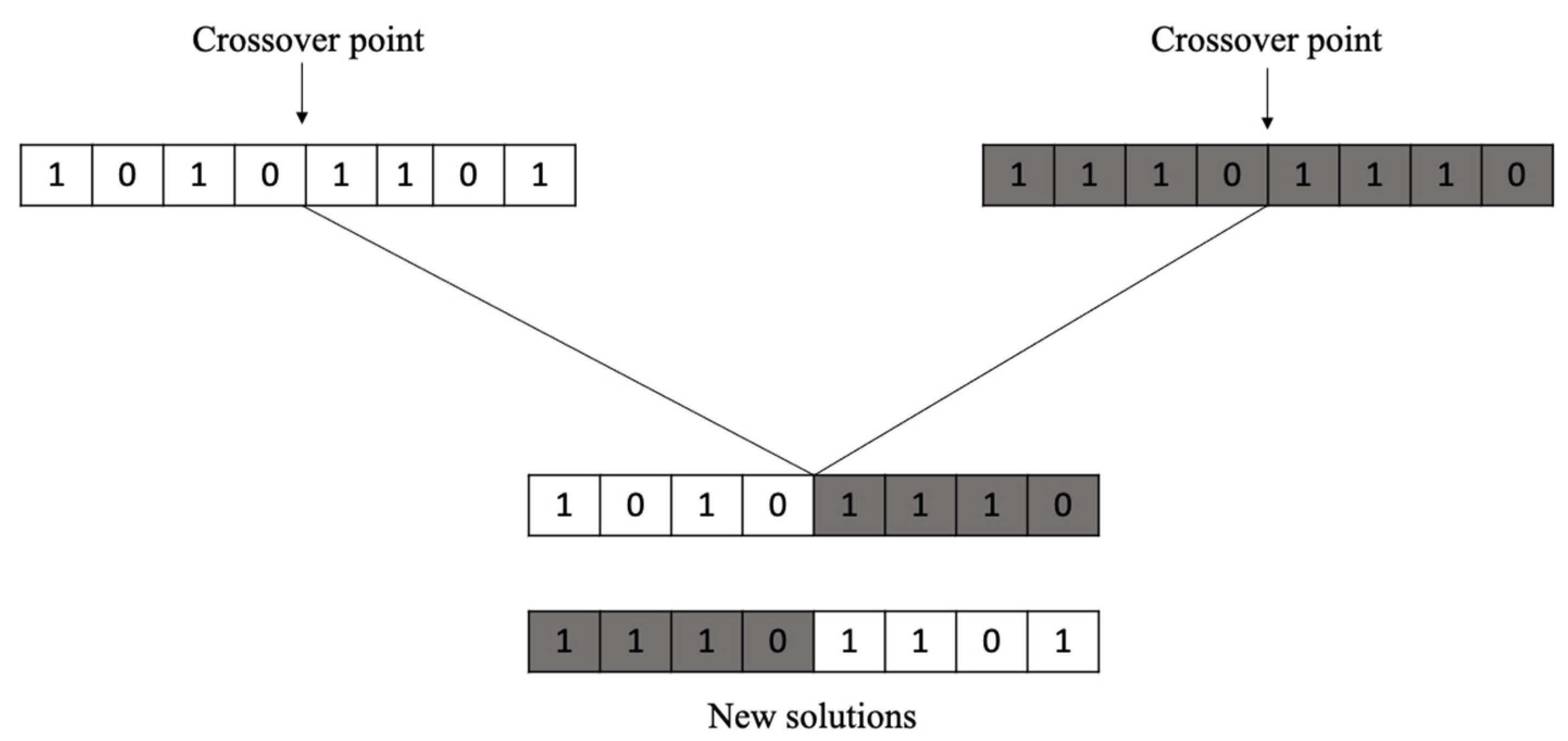
4.2. One-Point Crossover Operator

The one-point crossover operator generates two offsprings from two parents [23]. The process first defines a random cutting point cp in the range [0, n – 1]. After this, it split each parent vector into left and right sections, where for parent i, the left_i contains its values {s₀, …, s_cp}, and the right_i contains its values {s_cp+1, …, s_n–1}. Finally, it mixes the split sections to generate two new offsprings h₁, h₂, where h₁ uses left₁ and right₂, and h₂ uses left₂ and right₁. The parents are chosen at random. The steady-state approach only utilizes the first offspring h₁. The number of crossovers that are done is a defined parameter. Figure 2 shows an example of this operator.

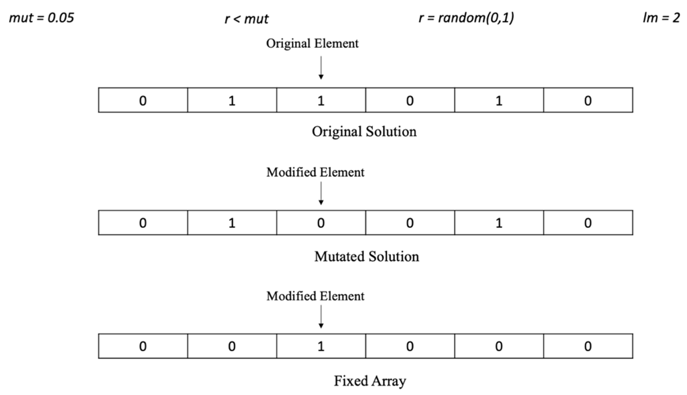
4.3. Uniform Mutation Operator

The uniform mutation operator generates a new solution for the mutation population from given a solution vector S = {s₀, s₁, …, s_n–1 } [24]. The process generates for each index i, for 0 ≤ i ≤ n − 1, a random number u in the range [0, 1], and if u < mut then the value of s_i changes from 1 to 0 or vice versa, otherwise the value s_i remains intact. The parameter mut is the mutation probability used by the operator. Figure 3 shows an example of the use of this mutation.

Another parameter of the operator is the number of new mutated solutions that must be generated. Usually, the solutions that undergo this process come from the crossover operator’s results; otherwise are randomly chosen.

4.4. Initial Population

A predefined number of randomly generated solutions are created to have an initial population. When a new random solution is generated, the objectives vector for the solution is determined and its feasibility is verified.

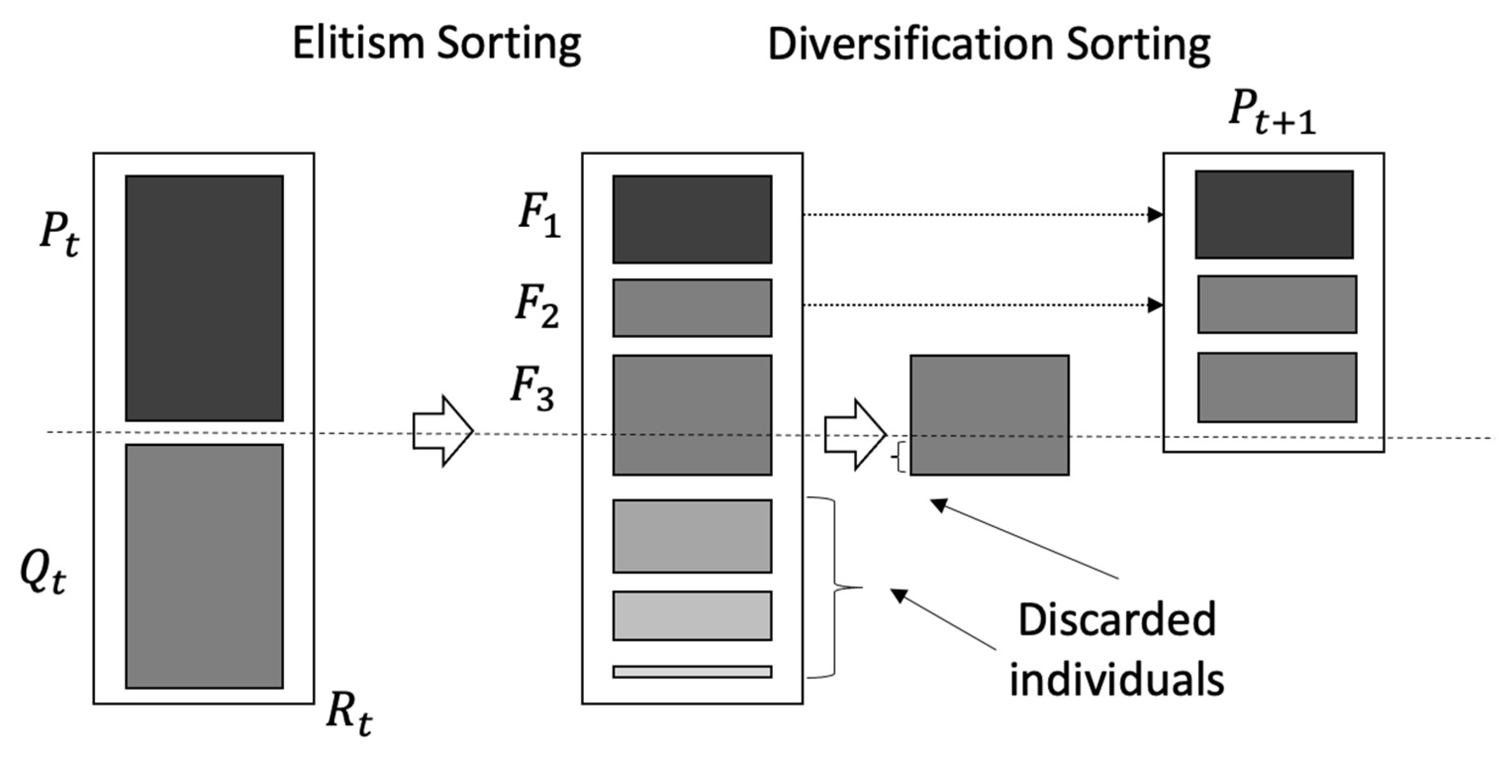
4.5. Population Sorting

This process consists of sorting the solutions of the population, and it is composed of two phases: (1) the elitist phase, which keeps the best solutions; and (2) the diversification phase, which ensures that there are solutions different enough to avoid local optima in the search process of the algorithm. The elitist phase is also known as non-dominated sorting. It consists of separating the population in fronts or sets of non-dominated solutions, making sure that the best solutions are always on the first front. The diversification phase sorts the solutions of a front according to the Crowding Distance indicator. The solutions in the best fronts are included in the population, and when a front cannot be completely inserted, the solutions with the worst crowding distances are discarded. Figure 4 shows both phases.

4.6. Non-Dominated Sorting

This process has two parts, and works on a given population. The first part constructs the first front with the set of non-dominated solutions identified from the comparison of vectors of objective values among all the population’ solutions. A solution is non-dominated if its vector of objective values is not dominated by any other. Note that the Pareto dominance uses real value vectors in its definition.

The second part builds the remaining fronts one by one. Each new front integrates those solutions that are only dominated by solutions in previously built fronts. The process repeats until no more fronts can be made.

4.7. Calculating the Crowding Distance

According to [22], this process orders the solutions in a front by their Crowding Distance (CD). The distance is a measure of the separation of the solutions, and it is relative to the normalized value of the objectives. The CD identify the solutions with extreme values on the objectives and put it first on the front. After that, the solutions order are according to their accumulated degree of separation per objective, the greatest the separation the better. For each objective, the CD computes the degree of separation using the ordered array of objective values resulting from the front; the solutions with the highest and smallest objective values will have a specific Crowding Distance value d equal to infinite ($\infty$), while the remaining solutions will be calculated by the following formula:

$$d_{I_j{}^m}=d_{I_j{}^m}+\frac{f_{m^{j+1}}^{I^m}-f_{m^{j-1}}^{I^m} }{f_m^{max}-f_m^{min}}$$

(42)

where d is the Crowding Distance, I is the solution position in the whole population in general, j is the solution position after the ordering by objective m within the front, f is the objective value and m is the current objective. The accumulation of Crowding Distance value d of all the objectives results in the final value of CD for each solution I.

4.8. Calculating the Spatial Spread Deviation (SSD)

The Spatial Spread Deviation (SSD) is a density estimator used to rearrange the solutions in a front, so the spread is not by a wide margin [25]. The method calculates for each solution the SSD value using a matrix of normalized distances between the solutions in the approximated front. The solutions are sorted from the lowest to highest SSD value in order to punish solutions according to their standard deviation and their proximity to their closest $k$-neighbors. The next three equations show how to calculate the SSD values, in the process i is the solution in the front for which the SSD is calculated, and j take values over all the solutions in the front except i.

$$temp1\left(i\right)=\frac{1}{n-1}\sqrt{{{\displaystyle \sum }}_{j=1}^n{\left(D\left(i,j\right)-\left(D_{max}-D_{min}\right)\right)}^2}\forall i \ne j$$

(43)

$$temp2\left(i\right)={{\displaystyle \sum }}_{jℰK}\frac{\left(D_{max}-D_{min}\right)}{D\left(i,j\right)}$$

(44)

$$SSD\left(i\right)=SS{D}_0\left(i\right)+temp1\left(i\right)+temp2\left(i\right)$$

(45)

where $D\left(i,j\right)$ is the distance from solution $i$ to solution $j$. $D_{\max }$ is the biggest distance between all the solutions and $D_{\min }$ is the closest distance between all the solutions. $K$ is the number of $k$ neighbors closest to solution $i$. $SS{D}_0$ is the initial value of SSD, which is -INF if the solution is at one of the ends of the front when the normalized values of the graded mean integration of the objective values are calculated.

4.9. Pseudocode of the T-NSGA-II Algorithm

The T-NSGA-II is based in the structure of the classic multi-objective algorithm NSGA-II proposed by Deb [22]. As previously described, the algorithm had several modifications to work with trapezoidal fuzzy numbers and the proposed MOPOP model. Algorithm 3 shows the detailed pseudocode of the algorithm T-NSGA-II.

Algorithm 3. T-NSGA-II pseudocode

INPUT: Instance with the trapezoidal parameters of the portfolio problem. OUTPUT: Approximated Pareto Front NOTE: The algorithm is called T-NSGA-II-CD when the Crowding Distance is used, and T-NSGA-II-SSD when is used the Spatial Spread Deviation. *************************************** 1. Create the initial population pop 2. Evaluate all the solutions in pop 3. Order pop using no-dominated Sorting 4. For all solutions in pop calculate Spatial Spread Deviation/Crowding distance

5. pop sorting due to fronts and Spatial Spread Deviation/CD 6. Main loop, until stopping condition is met *** Steady state approach: only one generated individual is considered to include in popc 7.  Create popc using crossover operator *********************************************************************** 8.  Create popm using mutation operator 9.  Join popc and popm to create popj 10. Evaluate solutions in popj and put feasibles in popf 11. Add popf to pop, and calculate objective functions 12. Order pop using no-dominated sorting 13. Calculate Spatial Spread Deviation/Crowding distance 14. pop sorting due to the front ranking and Spatial Spread Deviation/CD 15. Truncate pop to keep a population of original size 16. No-dominated sorting 17. Calculate Spatial Spread Deviation/Crowding distance of the individuals in pop 18. pop sorting due to front ranking and Spatial Spread Deviation/CD 19. End Main loop 20. Return (Front 0).  ***Approximated Pareto Front

5. T-FAME Algorithm

This section presents the design of all the components of the T-FAME algorithm. The algorithm adapts the FAME algorithm to work with the trapezoidal fuzzy numbers [25]. The input to the algorithm is an instance of MOPOP. The output is the approximate Pareto front for that instance. T-FAME updates the population, applying the steady-state approach to include in the population only one of the generated individuals. The following algorithm components are the same described in Section 4: the structure used to represent the solutions, the evaluation of a solution, the construction of the initial population, the sorting of the population, the non-dominated sorting process, and the density SSD estimator. The components described in this section are those not included in the previous description or with significant differences, such as the fuzzy controller, the additional genetic operators, and the structure used to store the approximated Pareto front.

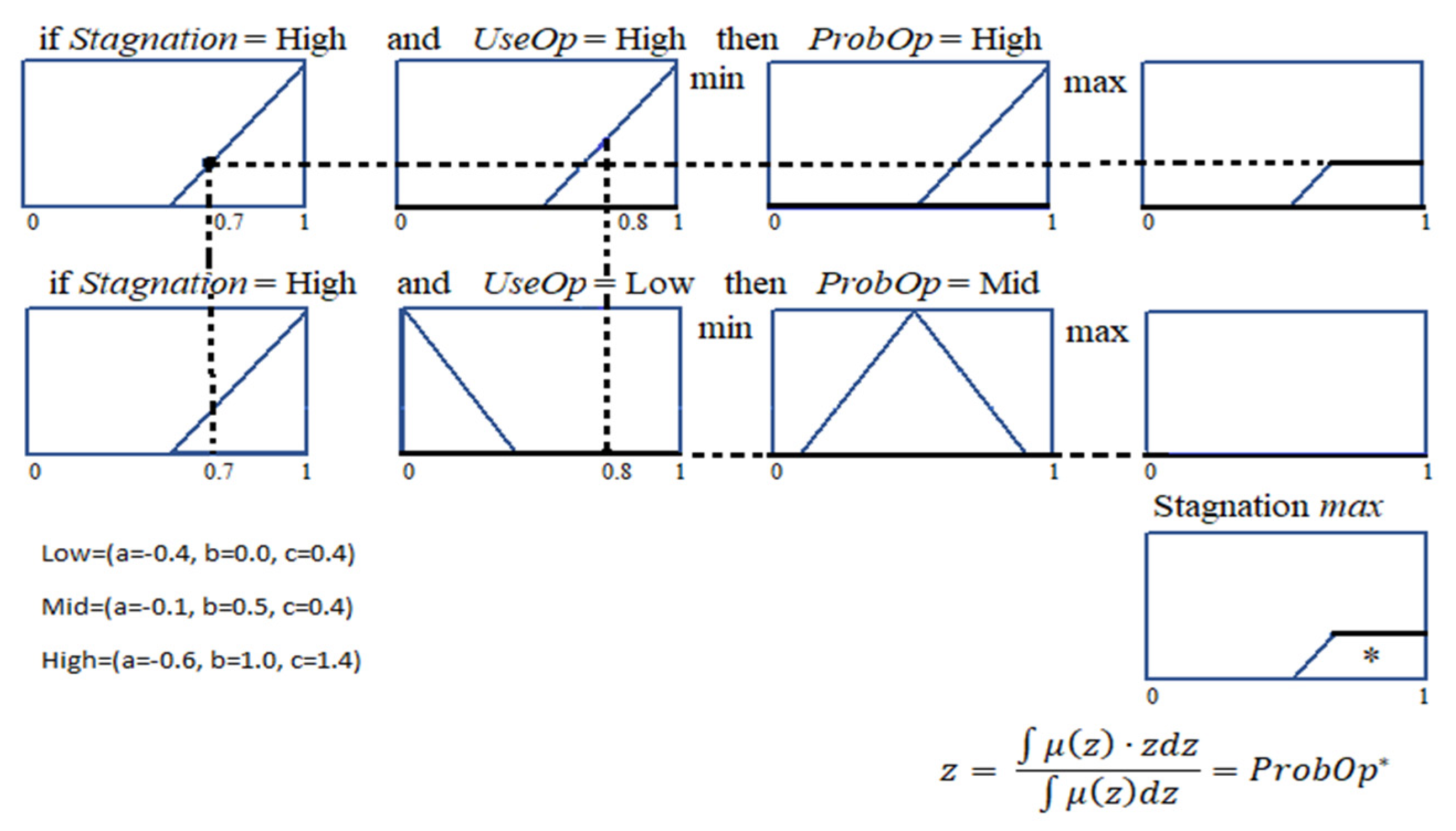
5.1. Fuzzy Controller

This section introduces an intelligent mechanism that allows an MOEA to apply different recombination operators at different search process stages. The use of different operators is dynamically adjusted according to their contribution to the search in the past. Intuitively, the idea is to favor operators generating higher quality solutions over others. For this purpose, the fuzzy controller dynamically tunes the probability selection of the available recombination operators [25].

The fuzzy controller uses a Mamdani-Type Fuzzy Inference System (FIS) [26] to compute the probability of applying the different operators. Fuzzy sets defined by membership functions represent the linguistic values of the model’s input and output variables. Regarding the inference, we use the approach originally proposed by Mamdani based on the “max min” composition: using the minimum operator for implication and maximum operator for aggregation. The aggregation of the consequents from the rules are combined into a single fuzzy set (output), to be defuzzified (mapped to a real value). A widely used defuzzification method is the centroid calculation, which returns the area’s center under the curve. We use triangular-shaped membership functions in all inputs and outputs,

$${\mathsf{\mu }}_{\mathrm{A}}\left(\mathrm{x}\right)=\{\begin{array}{cc}\hfill 0& x<a\hfill \\ \hfill \frac{x-a}{b-a}& x ϵ \left(a, b\right)\hfill \\ \hfill \frac{c-x}{c-b}& x ϵ \left(b, c\right)\hfill \\ \hfill 0& x>c\hfill \end{array}$$

(46)

the parameters a and c determine the “corners” of the triangle, and b determines the peak. A membership function ${\mathsf{\mu }}_{\mathrm{A}}\left(\mathrm{x}\right)$ maps real values of x with a degree of membership 0 ≤ ${\mathsf{\mu }}_{\mathrm{A}}\left(\mathrm{x}\right)$≤ 1. The used granularity levels were: Low (a = −0.4, b = 0.0, c = 0.4), Mid (a = 0.1, b = 0.5, c = 0.9) and High (a = 0.6, b = 1.0, c = 1.4).

The interaction of the fuzzy controller with the algorithm works as follows: Let Operators the set of genetic operators available. The evolutionary algorithm monitors the search process in a series of time windows, each of size Window. At the end of each time window, the algorithm sends to the fuzzy controller the real values of the input variables Stagnation and UseOp, and receives from the controller the real value of the output variable ProbOp.

Each of the fuzzy variables has associated the fuzzy linguistic values: High, Mid and Low. Then the membership functions of the fuzzy variable Stagnation are: ${\mu }_{Stagnation=High}\left(x\right), {\mu }_{Stagnation=Mid}\left(x\right) and {\mu }_{Stagnation=Low}\left(x\right).$ In a similar way, the membership functions are defined for the variables UseOp and ProbOp.

To show how works the fuzzification process consider that the received real values of the input variables are Stagnation = 0.7 and UseOp = 0.8.

The fuzzified values for the Stagnation variable are the membership degrees: ${\mu }_{Stagnation=High}\left(0.7\right), {\mu }_{Stagnation=Mid}\left(0.7\right) y {\mu }_{Stagnation=Low}\left(0.7\right).$

For the UseOp variable the fuzzified values are the membership degrees: ${\mu }_{UseOp=High}\left(0.8\right), {\mu }_{UseOp=Mid}\left(0.8\right) y {\mu }_{UseOp=Low}\left(0.8\right).$ All the membership degrees are values in the interval (0,1).

Now the FIS includes a set of fuzzy rules which are specified in terms of the fuzzy variables, the linguistic values, and a set of logic operators. To continue with the previous example, consider that the fuzzy rules in the FIS are:

$$R_1: If Stagnation=High and UseOp=High then ProbOp=High$$

(47)

$$R_2: If Stagnation=High and UseOp=Low then ProbOp=Mid$$

(48)

Once the fuzzification of the inputs is done, the next process is to evaluate the antecedents of the rules $R_{1 }and R_2,$ determining the following values:

$$k_1=min({\mu }_{Stagnation=High}\left(0.7\right),{\mu }_{UseOp=High}\left(0.8\right))$$

(49)

$$k_2=min({\mu }_{Stagnation=High}\left(0.7\right),{\mu }_{UseOp=Low}\left(0.8\right))$$

(50)

In the rule evaluation, the min operator is associated with the logic operator and, and the max operator is associated to the logic operator or.

Now the membership functions of the consequents of the rules must be determined. For each rule an operator of implication is applied to the antecedent value obtained in the previous process and to the consequent of the rule, to determine the membership function of the conclusion of the rule. The min operator is used to implement the implication logic operator, which truncates the membership function of the rule’s consequent. For example, the truncated membership functions of the consequents are the following:

$${\mu }^{*}{}_{ProbOp=High}\left(z\right)=\min \left({\mu }_{ProbOp=High}\left(z\right),k_1\right) z \in \left(0,1\right)$$

(51)

$${\mu }^{*}{}_{ProbOp=Mid}\left(z\right)=\min \left({\mu }_{ProbOp=Mid}\left(z\right),k_2\right)z \in \left(0,1\right)$$

(52)

Now the truncated membership functions are integrated using an aggregation operator to create a new membership function, which is the controller’s fuzzy output. The aggregation operators that are frequently used are max and sum.

For the example, the max operator is used to determine the aggregated membership function, which is the following:

$${\mu }^{**}\left(z\right)=\max \left({\mu }^{*}{}_{Z=A}\left(z\right), {\mu }^{*}{}_{Z=M}\left(z\right)\right) z \in \left(0,1\right)$$

(53)

Finally, the defuzzification of the fuzzy output obtained is done. In this step a real number is associated to the aggregated membership function, which is the output of the inference process. In the previous example, the center of the area under the curve of the aggregated membership function is used to defuzzify the output of the controller as following:

$$z=\frac{{{\displaystyle \int }}^{ }{\mu }^{**}\left(z\right)zdz}{{{\displaystyle \int }}^{ }{\mu }^{**}\left(z\right)dz}$$

(54)

Figure 5 graphically shows the fuzzy inference process for the example described.

All of the controller rules are of the type: Antecedent AND Antecedent then Consequent. The fuzzy rules were designed to have soft changes in the input variables (Stagnation and UseOp), to avoid abrupt changes in the output variable (ProbOp). The configuration was manually done by observing the surface that these three variables generated [25].

Table 2. Fuzzy controller rules.

AND Antecedents		Consequent
Stagnation	Utilization	ProbOp
High	High	Mid
High	Mid	Low
High	Low	Mid
Mid	High	Mid
Mid	Mid	Low
Mid	Low	Mid
Low	High	High
Low	Mid	Mid
Low	Low	Low

shows the rules of the fuzzy controller.

The Algorithm 4 shows the structure of the fuzzy controller used in the fuzzy controller implementation with the Java Library Fuzzy Lite 6.0.

Algorithm 4. Fuzzy controller structure.

[System]

Name=‘FuzzyController ‘

Type=‘mamdani’

Version=2.0

NumInputs=2

NumOutputs=1

NumRules=9

AndMethod=‘min’

OrMethod=‘max’

ImpMethod=‘min’

AggMethod=‘max’

DefuzzMethod=‘centroid’

[Input1]

Name=‘Stagnation’

Range=[0 1]

NumMFs=3

MF1=‘Low’:’trimf’,[−0.4 0 0.4]

MF2=‘Mid’:’trimf’,[0.1 0.5 0.9]

MF3=‘High’:’trimf’,[0.6 1 1.4]

[Input2]

Name=‘UseOp’

Range=[0 1]

NumMFs=3

MF1=‘Low’:’trimf’,[−0.4 0 0.4]

MF2=‘Mid’:’trimf’,[0.1 0.5 0.9]

MF3=‘High’:’trimf’,[0.6 1 1.4]

[Output1]

Name=‘ProbOp’

Range=[0 1]

NumMFs=3

MF1=‘Low’:’trimf’,[−0.4 0 0.4]

MF2=‘Mid’:’trimf’,[0.1 0.5 0.9]

MF3=‘High’:’trimf’,[0.6 1 1.4]

[Rules]

3 3, 2 (1) : 1

3 2, 1 (1) : 1

3 1, 2 (1) : 1

2 3, 2 (1) : 1

2 2, 1 (1) : 1

2 1, 2 (1) : 1

1 3, 3 (1) : 1

1 2, 2 (1) : 1

1 1, 1 (1) : 1

In the [Rules] section, the first and second columns contain the linguistic values of the two input variables (1-Low, 2-Mid, 3-High), the third column is the weight of the rules, and the last one indicates the logic operator used in the rule (1-and, 2-or).

The interaction of the fuzzy controller with the algorithm works as follows: Let Operators the set of genetic operators available. The T-FAME algorithm searches in the solutions space in time windows of size Window, each time window the algorithm performs Window iterations. At the end of each time window, the algorithm sends to the fuzzy controller the values of the input variables Stagnation and UseOp[i] for all i ∈ Operator. For each pair of input values, a Fuzzy Inference generates ProbOp[i] for all i ∈ Operator. This process is done for the T-FAME algorithm with the following pseudocode where v is the windows counter:

If (v == Window) then

$$\forall iϵ \left\{1,2,\dots .SizeOP\right\}$$

$$38. ProbOp\left(i\right)=\mathrm{Fuzzy}Controller\left(Stagnation, UseOp\left(i\right)\right);$$

39. v =0; Stagnation = 0;

40. Endif

The line numbers are those that appear in the T-FAME algorithm pseudocode included in Section 6.4. Notice that in lines 37 and 38, the algorithm uses the fuzzy controller to update all the available recombination genetic operators’ selection probability.

The Stagnation value is shared for all the operators, and it is an indicator of the evolution of the search in the current time window. This is a normalized value that is increased by 1.0/Window each time the generated solution cannot enter the set where the non-dominated solutions are kept and reset when the time window is over. UseOp[i] is a normalized value that is increased by 1.0/Window every time the operator i is used.

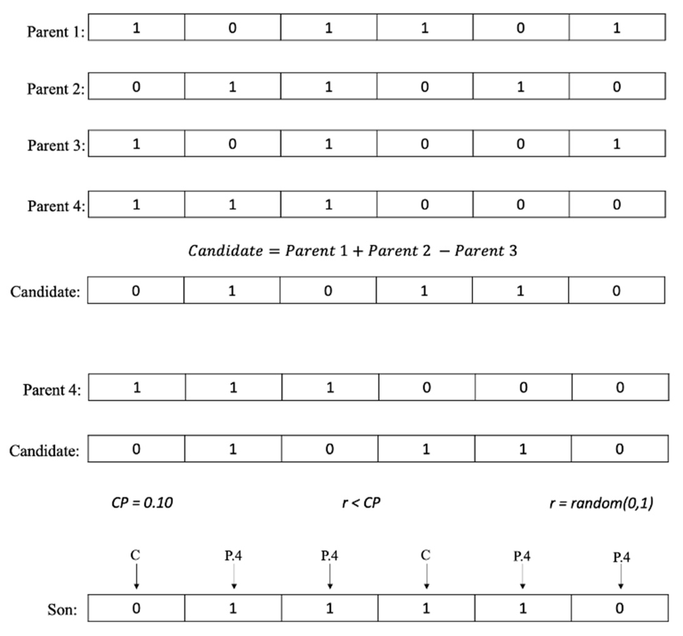
5.2. Additional Genetic Operators

Four operators are used in T-FAME to create new solutions: One-point crossover, Uniform Mutation, Fixed Mutation, and Differential Evolution. Two of these operators (One-point crossover and Uniform Mutation) are the same ones that are used on T-NSGA-II, and they are already described in the previous section.

Differential Evolution: This method was proposed by Rainer [27], and its implementation was based on [28]. It uses the four parents obtained with the tournament method. The first part of the process consists of creating a new solution called Candidate using Parent 1, Parent 2, and Parent 3, this solution is obtained by doing a binary addition of the parents. Figure 6 shows an example of how this operator works.

Once the Candidate is calculated, a binary crossover operator is done between the candidate and Parent 4 to create a new solution called Son, this binary crossover operator is different from the one-point crossover operator described previously, and it uses a parameter called crossover percentage (CP). The binary crossover operator consists of the following: For each array index, a random number between 0 and 1 is generated, if that number has a lesser value than CP, then that index receives the value of the Candidate, if this is not the case, then that index receives the value of Parent 4.

Once the new solution Son is completed, a dominance test is done between Son and Parent 4, if the objective values of Parent 4 dominate the objective values of Son, then Parent 4 proceeds to be the new solution, but if this is not the case, then Son proceeds to be the new solution.

Fixed Mutation: This method is very similar to the uniform mutation operator that was described previously. The main difference lies in the fact that the whole process is done in a loop until n mutations are made, where n is a parameter previously defined. This operator also makes sure that no element in the solution is changed twice or more times, this is done by using a fixed array to keep track of the changed elements in the solution. Figure 7 shows an example of the Fixed Mutation operator.

5.3. Used Structures to Store the Population and the Approximated Pareto Front

The algorithm uses the structure pop to maintain a solutions population, which contains the following information for each solution i:

• V(i): vector binary associated to the solution i.
• O₁(i) and O₂(i): values of the two objectives of the solution i, converted to GMI values.
• r(i): ranking of the solution i is the number of the front in which is located.
• Dominated(i): solutions dominated by the solution i.
• Domines(i): solutions that dominates to solution i.
• CD (i): Crowding Distance value of the solution i.
• SSD(i): Spatial Spread Deviation value of solution i.

The structure Front is used to store the approximated Pareto front, which contains the following information for each stored solution i:

• V(i): vector binary associated to the solution i.
• O(i): real vector of the graded mean values of the fuzzy triangular objectives of the solution V(i).
• r(i): ranking of the solution i is the number of the front in which is located.
• Dominated(i): solutions dominated by the solution i.
• Domines(i): solutions that dominates to solution i.
• SSD (i): Spatial Spread Deviation value of the solution i.

5.4. T-FAME Algorithm Pseudocode

This section presents the pseudocode for the algorithm T-FAME in Algorithm 5.

Algorithm 5. T-FAME pseudocode

INPUT: Instance with the trapezoidal parameters of the portfolio problem. OUTPUT: Approximated Pareto front Variables pop: Population of solutions (binary vectors) Front: Limited sized set were no-dominated solutions are kept Operator: Vector of size SizeOP that contains the index of the available operators Parents: Vector of size NParents that contains the chosen parents ProbOp(i): Probability that operator i has of being chosen, it has values between 0 and 1 UseOp(i): Normalized Indicator of how much operator i has been used, it has values between 0 and 1 Stagnation: Normalized indicator of the number of generated solutions that couldn’t be inserted into Front, because they were either dominated solutions or there was not space available for them, it can have values between 0 and 1. MAXEVAL: Maximum number of evaluations of the objective function (stopping criterion) Window: Size of the time window. eval: Accumulator of the evaluations of the objective function v: Counter of the time windows that have elapsed Functions

CreateaSon(Operator(i), Parents): Generates one solution using the previous chosen operator i with the chosen parents (Steady state) Evaluate(Son): Calculates the objective values of Son and verify feasibility FuzzyController(Stagnation, UseOp(i)): Function that invokes the fuzzy controller with Stagnation and UseOp(i) as input values and returns the probability of selection of all the operators no-dominated_sortingSSD(NewPop): Sorts the fronts of NewPop by dominance and uses as ranking the SSD values of the solutions. EliminateWorstSolutionSSD(NewPop): Eliminates from the last front of NewPop the solution with the worst SSD, and assign NewPop to pop.

**************************************************************** 1. Create(pop) **Create random population 2. Front=NoDominated(pop) **Insert in Front the no-dominated solutions of pop 3. $\forall iϵ \left\{1,2,\dots .,SizeOP\right\} ProbOp\left(i\right)=$1, UseOp(i)=0 4. v =0; Stagnation = 0; eval=0; 5. while (eval<MAXEVAL) do. **** Stop condition ** Chose |NParents| ** With a probability $\beta$ each parent is taken from Front to intensify) and with 1-$\beta$ from pop to diversify. 6.   $\forall iϵ \left\{1,2,..\left|NParents\right|\right\}$ do 7.       if (RandomDouble(0,1) $\le \beta$) then **The parent is chosen from Front 8.          Parents[i] ← TournamentSSD(Front) 9.       Else **The parent is chosen from pop 10.         Parents[i] ← TournamentSSD(pop) *** Roulette to choose an operator with the selection probabilities of the operators 11.     sum=0 12.     $i=Random\left(1,2,\dots ,NParents\right)$ 13.     sum=sum+ProbOp(i) 14.     while (sum>0) do 15.        $i=Random\left(1,2,\dots ,NParents\right)$ 16.        sum=sum+ProbOp(i) ********** ***** The chosen operator is associated with the last value of i ** ***Steady state approach 17.       Son ← CreateaSon(Operator(i), Parents) **** Get the objective vector values corresponding to Son and verify feasibility. 18.       Evaluate(Son) 19.       eval=eval+1 20.       UseOp(Operator(i)) = UseOp(Operator(i))+ 1 . 0/ Window 21.       v=v+1 ******************************* 22.        If (Son dominates a set S of solutions in Front) 23.          then { Front=Front\S; Front=Front ${{\displaystyle \cup }}^{ }$Son} 24.          else If ($\exists$ s Front such that s dominates Son) 25.             then (Stagnation= Stagnation+1.0/ Window) 26.             else if (Sizeof(Front)<100) 27.                 then (Front=Front ${{\displaystyle \cup }}^{ }$Son) 28.                 else { 29.                    Front=Front ${{\displaystyle \cup }}^{ }$Son ** Front[1 00]=Son 30.                    Calculate SSD for all the solutions in Front 31.                    Sort the solutions in Front in ascending order by SSD 32.                    Eliminate the solution in Front with worst SSD:Front[100] 33.                    If (Son Front) 34.                    then Stagnation= Stagnation+1.0/ Window 35.                  } 36.           If (v == Window) then **** The Fuzzy Controller is used to update the selection probability ****of all the operators 37.            $\forall iϵ \left\{1,2,\dots SizeOP\right\}$ 38.            $ProbOp\left(i\right)=\mathrm{Fuzzy}Controller\left(Stagnation, UseOp\left(i\right)\right)$ 39.             v =0;  Stagnation = 0; 40.           End if 41.          pop=pop ${{\displaystyle \cup }}^{ }$Son 42.           NewPop=pop 43.           no-dominated_sortingSSD(NewPop) 44.          pop ← EliminateWorstSolutionSSD(NewPop) 45. End while 46. Return(Front) *** Approximated Pareto front generated

6. Experimental Results

Two experiments were done in order to evaluate the performance of the proposed algorithms. The tested steady-state algorithms were T-NSGA-II-CD, T-NSGA-II-SSD, and T-FAME. The first experiment was done to make sure the algorithms were implemented correctly, while the second experiment was done to compare the performance between them using performance metrics.

The software and hardware platforms that were used for these experiments include Intel Core i5 1.6GHz processor, RAM 4GB, and IntelliJ IDEA CE IDE.

6.1. Performance Metrics Used

In order to measure the performance of each algorithm, two metrics were used: hypervolume [28] and generalized spread [29].

Hypervolume is the n-dimensional solution space volume that is dominated by the solutions in the reference set. If this space is big, then that means that the set is close to the Pareto Front. It is desirable for the indicator to have large values. Generalized Spread calculates the average of the distances of the points in the reference set to their closest neighbor. If this indicator has small values, then that means the solutions in the reference set are well distributed.

6.2. Experimental Setup

In order to configure the algorithms used in this work, the parameter values reported in the state-of-the-art were considered. The parameter value for the maximum number of evaluations was determined after a preliminary experimental phase. The comparison of all the algorithms, under the same operation conditions, utilizes a steady-state approach, using the dominant son.

Table 3. T-NSGA-II-SSD parameters.

Parameter	Value
Evaluation of the objective function	5000
Population Size	50
Crossover population %	70
Mutation population %	40
Mutation %	5

and

Table 4. T-FAME parameters.

Parameter	Value
Evaluation of the objective function	5000
Population Size	25
Front Size	100
Tournament Size	5
Number of parents	4
Window Size	13
Differential Evolution Crossover %	10
Number of mutations in FM	2
Front choice probability ($\beta )$	0.9

show the values of the parameters used in the algorithms. The configuration of algorithm T-NSGA-II-SSD is the same one as T-NSGA-II-CD, however, it uses Spatial Spread Deviation instead of Crowding Distance as its density estimator.

6.3. Experiment 1. Validating the Implemented Algorithms

For this experiment, an instance named o2p25_rand was used, this instance was originally created for POP with intervals, which was converted in a trapezoidal fuzzy instance by adding two parameters to the intervals. The optimum Pareto Front was obtained using an exhaustive algorithm, and approximate fronts were obtained with T-NSGA-II-CD, T-NSGA-II-SSD, and T-FAME algorithms. All algorithms solve the MOPOP with Fuzzy Parameters and use a steady-state election mechanism, creating one solution from the genetic operators’ application. This adaptation from FAME has an advantage over algorithms using the classic generational approach in genetic algorithms.

The purpose of this experiment is to validate the correct operation of the implemented algorithms in the project. In the experiment, the fronts are generated, and they are compared to the optimum front, in order to determine if the algorithms are generating similar fronts. All the fronts that were generated are shown in

Table 5. Generated fronts of the algorithms with instance o2p25_rand.

Pareto Optimal Front		T-NSGA-II-CD		T-NSGA-II-SSD		T-FAME
O2	O1	O2	O1	O2	O1	O2
3530	78,510	3465	81,155	3425	81,285	3530
3805	62,350	4245	66,240	4400	77,480	3715
3825	76,360	3840	75,650	3860	74,485	3750
3840	70,035	3870	68,610	4240	73,425	3775
3865	77,020	3490			70,350	4005
3965	66,605	4070			66,850	4375
3980	62,755	4090			59,865	4385
4000	77,900	3490
4025	77,920	3485
4035
4060
4065
4120
4150
4215
4235
4240
4260
4310
4375
4400
4435
4460

. Each front is shown in two columns that contain the values of the two objectives that were originally Trapezoidal Fuzzy numbers, but they were converted into real numbers with the transformation based on GMI. The graph the fronts uses the GMI values obtained from the objectives.

It is worth nothing that, in Figure 8, the approximated fronts are relatively close and below the optimum front. Also, observe that the T-NSGA-II-SSD and T-FAME algorithms managed to reach some optimum solutions. Finally, note that the T-FAME algorithm has a good distribution between its solutions.

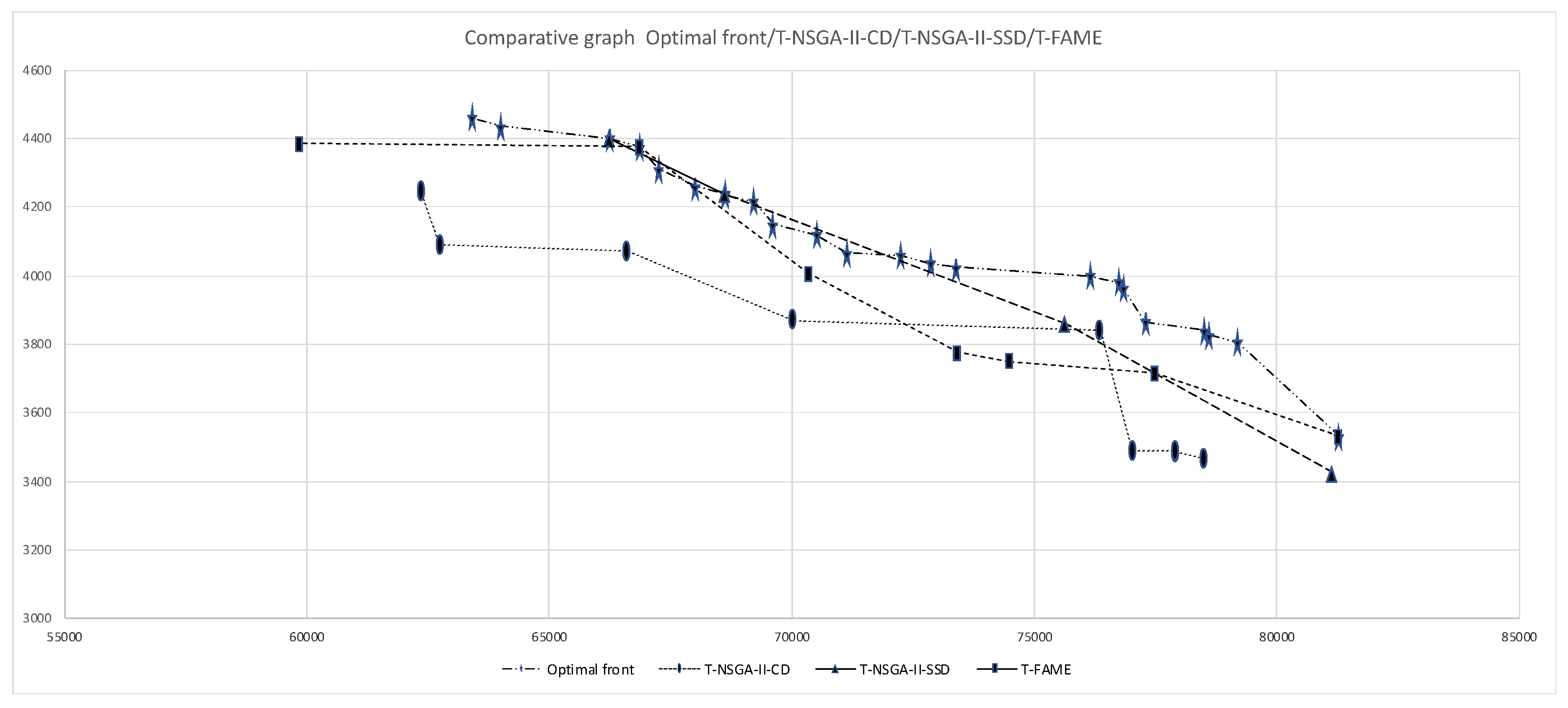
6.4. Experiment 2. Evaluating the Performance of the Algorithms with Instances of 25 Projects

This experiment evaluates the performances of algorithms T-NSGA-II-CD, T-NSGA-II-SSD, and T-FAME, and utilizes 13 instances with 2 objectives and 25 projects. In order to compare the performance between the three algorithms, each algorithm was executed 30 times per instance. The performance metrics used were hypervolume and generalized spread. For each instance, the reference set contains the non-dominated solutions obtained from the combination of the 30 generated fronts. The computation of the metrics uses the reference set as an approximation to the optimum Pareto Front. The computation of the median value and interquartile ranges uses the metric values of the 30 instances sorted in ascending order. With the sorted array, the median value was the average of the metric values from positions 15 and 16. At the same time, the interquartile ranges correspond to those in positions 23 and 8, corresponding to the 75% and 25% of the metrics values, respectively. The median value and the interquartile ranges are used instead of the average and the standard deviation because they are less sensitive to extreme values. The experiment performs a hypothesis test to validate the obtained results. The hypothesis was proven using the parametric t student test on those data sets that passed the normality and homoscedasticity tests and using the non-parametric Wilcoxon signed-rank test on those that do not. Both tests apply a confidence level of 95%, pairing T-FAME with each of the other two algorithms.

Table 6. Hypervolume normality test, the null hypothesis is that the samples follow a normal distribution which is accepted (a) when p-value < 0.05 and rejected (r) otherwise.

	T-NSGA-II-CD			T-NSGA-II-SSD			T-FAME
Instance	Statistic	p-Value	R	Statistic	p-Value	R	Statistic	p-Value	R	Tests
o2p25_0T	0.9429	0.1089	a	0.83756	0.00034	r	0.96919	0.51737	a	t,W
o2p25_1T	0.93655	0.07348	a	0.92817	0.04391	r	0.97408	0.65561	a	t,W
o2p25_2T	0.92141	0.02918	r	0.95491	0.22837	a	0.96987	0.53551	a	W,t
o2p25_3T	0.94311	0.11035	a	0.90566	0.01159	r	0.94528	0.12625	a	t,W
o2p25_4T	0.95413	0.21782	a	0.93505	0.06696	a	0.89022	0.00488	r	W,W
o2p25_5T	0.86113	0.00107	r	0.89584	0.00665	r	0.94768	0.14643	a	W,W
o2p25_6T	0.9023	0.00956	r	0.89233	0.00548	r	0.96519	0.41715	a	W,W
o2p25_7T	0.94961	0.16508	a	0.86559	0.00134	r	0.92644	0.03953	r	W,W
o2p25_8T	0.92385	0.0338	r	0.91474	0.01963	r	0.85737	0.00089	r	W,W
o2p25_9T	0.94965	0.16541	a	0.89673	0.00699	r	0.97209	0.59792	a	t,W
o2p25_10T	0.92989	0.04877	r	0.78913	0.00004	r	0.97575	0.70469	a	W,W
o2p25_11T	0.93191	0.05518	a	0.95357	0.21047	a	0.96642	0.44633	a	t,t
o2p25_12T	0.94626	0.13411	a	0.95055	0.17491	a	0.98323	0.9033	a	t,t
o2p100_1T	0.96346	0.37847	a	0.96637	0.44525	a	0.98333	0.90552	a	t,t
o2p100_2T	0.95885	0.28944	a	0.98951	0.98844	a	0.9737	0.64441	a	t,t
o2p100_3T	0.93272	0.05801	a	0.9821	0.87827	a	0.94779	0.14745	a	t,t
o2p100_4T	0.78768	0.00004	r	0.78085	0.00003	r	0.89022	0.00488	r	W,W
o2p100_5T	0.95289	0.20189	a	0.94588	0.13101	a	0.93478	0.06586	a	t,t
o2p100_6T	0.94043	0.09341	a	0.93788	0.07976	a	0.95224	0.194	a	t,t
o2p100_7T	0.97249	0.60937	a	0.99025	0.99229	a	0.94017	0.0919	a	t,t
o2p100_8T	0.96892	0.51019	a	0.98362	0.9115	a	0.96805	0.48728	a	t,t
o2p100_9T	0.57553	0	r	0.52513	0	r	0.71502	0	r	W,W

,

Table 7. Hypervolume homoscedasticity test, the null hypothesis is that all the input populations come from populations with equal variances, which is accepted (a) when p-value < 0.05 and rejected (r) otherwise. We can observe that the null hypothesis is accepted (a) for all the instances. The parametric t student test can be applied for all the instances that accept the null hypothesis in the normality tests.

Instance	Statistic	p-Value	R
o2p25_0T	8.46563	0.00044	a
o2p25_1T	17.23159	0	a
o2p25_2T	8.53517	0.00041	a
o2p25_3T	11.87763	0.00003	a
o2p25_4T	7.1698	0.00131	a
o2p25_5T	7.60431	0.0009	a
o2p25_6T	7.19194	0.00129	a
o2p25_7T	2.20562	0.11631	a
o2p25_8T	8.18222	0.00055	a
o2p25_9T	4.45024	0.01445	a
o2p25_10T	3.63843	0.03037	a
o2p25_11T	3.98587	0.02207	a
o2p25_12T	9.90574	0.00013	a
o2p100_1T	0.27401	0.76098	a
o2p100_2T	2.14347	0.1234	a
o2p100_3T	0.29369	0.74624	a
o2p100_4T	1.79147	0.17281	a
o2p100_5T	5.98972	0.00365	a
o2p100_6T	1.09354	0.33959	a
o2p100_7T	2.30064	0.10626	a
o2p100_8T	4.20117	0.01812	a
o2p100_9T	1.39539	0.25322	A

,

Table 8. Generalized Spread normality test, the null hypothesis is that the samples follow a normal distribution which is accepted (a) when p-value < 0.05 and rejected (r) otherwise.

	T-NSGA-II-CD			T-NSGA-II-SSD			T-FAME
Instance	Statistic	p-Value	R	Statistic	p-Value	R	Statistic	p-Value	R	Tests
o2p25_0T	0.92895	0.04606	r	0.97607	0.71429	a	0.9784	0.78164	a	W,t
o2p25_1T	0.98376	0.91432	a	0.95618	0.24658	a	0.97193	0.59314	a	t,t
o2p25_2T	0.98074	0.84479	a	0.97925	0.8053	a	0.96813	0.48946	a	t,t
o2p25_3T	0.9215	0.02934	r	0.9225	0.03116	r	0.96419	0.39452	a	W,W
o2p25_4T	0.95187	0.18969	a	0.96214	0.35091	a	0.68255	0	r	W,W
o2p25_5T	0.96913	0.51555	a	0.95677	0.25552	a	0.92403	0.03416	r	W,W
o2p25_6T	0.87495	0.00216	r	0.97296	0.62306	a	0.958	0.27513	a	W,t
o2p25_7T	0.94053	0.094	a	0.95631	0.24864	a	0.94784	0.14792	a	t,t
o2p25_8T	0.9648	0.40819	a	0.95561	0.23827	a	0.94282	0.10833	a	t,t
o2p25_9T	0.97001	0.53934	a	0.97168	0.58607	a	0.9686	0.50171	a	t,t
o2p25_10T	0.92765	0.04254	r	0.96999	0.53902	a	0.97623	0.71907	a	W,t
o2p25_11T	0.91446	0.01932	r	0.96986	0.53537	a	0.95816	0.27785	a	W,t
o2p25_12T	0.95492	0.22856	a	0.98402	0.91939	a	0.95432	0.22029	a	t,t
o2p100_1T	0.92495	0.03611	r	0.92054	0.02771	r	0.94295	0.10926	a	W,W
o2p100_2T	0.9812	0.85642	a	0.95454	0.22326	a	0.95353	0.21003	a	t,t
o2p100_3T	0.92278	0.03169	r	0.86033	0.00103	r	0.96482	0.40857	a	W,W
o2p100_4T	0.65395	0	r	0.79925	0.00006	r	0.68255	0	r	W,W
o2p100_5T	0.91266	0.01738	r	0.86347	0.0012	r	0.96541	0.4223	a	W,W
o2p100_6T	0.90797	0.01323	r	0.91912	0.02544	r	0.90857	0.01369	r	W,W
o2p100_7T	0.89328	0.00578	r	0.89889	0.00789	r	0.96516	0.41655	a	W,W
o2p100_8T	0.94824	0.15169	a	0.96578	0.43096	a	0.96071	0.32297	a	t,t
o2p100_9T	0.49141	0	r	0.68971	0	r	0.68313	0	r	W,W

and

Table 9. Generalized Spread homoscedasticy test, the null hypothesis is that all the input populations come from populations with equal variances, which is accepted (a) when p-value < 0.05 and rejected (r) otherwise. Observe that the null hypothesis is accepted (a) for all the instances. The parametric t student test can be applied for all the instances that accept the null hypothesis in the normality tests.

Instance	Statistic	p-Value	R
o2p25_0T	0.33509	0.71619	a
o2p25_1T	3.11548	0.04934	a
o2p25_2T	5.44373	0.00592	a
o2p25_3T	7.81001	0.00076	a
o2p25_4T	0.38001	0.68498	a
o2p25_5T	3.01271	0.05431	a
o2p25_6T	1.58378	0.21106	a
o2p25_7T	10.87966	0.00006	a
o2p25_8T	1.51668	0.22518	a
o2p25_9T	19.54345	0	a
o2p25_10T	5.78604	0.00437	a
o2p25_11T	7.0285	0.00148	a
o2p25_12T	15.29209	0	a
o2p100_1T	8.48884	0.00043	a
o2p100_2T	9.53401	0.00018	a
o2p100_3T	3.46674	0.0356	a
o2p100_4T	1.42075	0.24708	a
o2p100_5T	3.96176	0.02256	a
o2p100_6T	4.19408	0.01824	a
o2p100_7T	4.62372	0.01235	a
o2p100_8T	5.30008	0.00673	a
o2p100_9T	0.90643	0.40774	a

show the results of the normality and homoscedasticity tests done for all the instances used in this work (25 and 100 projects) and the metrics of hypervolume and generalized spread. Table 6 and Table 8 show in the last column pairs (i,j), which indicate that the comparison of T-NSGA-II-CD and T-FAME uses test i, and the comparison T-NSGA-II-SSD and T-FAME uses test j. The values t and W in (i, j) stand for t student test and Wilcoxon test. This work tests each instance separately.

Table 10. Results with the hypervolume metric.

Hypervolume
Instance	T-NSGA-II-CD	T-NSGA-II-SSD	T-FAME
o2p25_0T	0.47470.0858⋁*	0.31830.3853⋁	0.20240.2491
o2p25_1T	0.38070.0510⋁*	0.24600.2325⋁	0.20030.2876
o2p25_2T	0.35910.0614⋁	0.24670.2042⋁*	0.16130.1526
o2p25_3T	0.28320.0549⋁*	0.27700.2311⋁	0.13450.1646
o2p25_4T	0.35100.0812⋁	0.28360.1489⋁	0.18750.1673
o2p25_5T	0.26350.0383⋁	0.15290.1495⋁	0.10700.1048
o2p25_6T	0.37970.0609⋁	0.24650.1870⋁	0.13800.2060
o2p25_7T	0.23480.2446⋁	0.28160.3644⋁	0.14270.1694
o2p25_8T	0.25740.0664⋁	0.18380.2259⋁	0.16300.1747
o2p25_9T	0.40260.1184⋁*	0.24490.2455⋁	0.15390.1615
o2p25_10T	0.25800.0710⋁	0.14510.1566⋁	0.11260.1070
o2p25_11T	0.39180.0946⋁*	0.23270.1687=*	0.18760.1657
o2p25_12T	0.29340.0708⋁*	0.26210.2174=*	0.23520.1969

shows the performance results with the hypervolume metric, and

Table 11. Results with the generalized spread metric.

Generalized Spread
Instance	T-NSGA-II-CD	T-NSGA-II-SSD	T-FAME
o2p25_0T	0.61780.1985⋀	0.41900.1534 = *	0.41540.2064
o2p25_1T	0.73440.1685⋀*	0.44770.1289 = *	0.46610.1128
o2p25_2T	0.60650.2078⋀*	0.39290.1025 = *	0.39830.1047
o2p25_3T	0.72760.2387⋀	0.51810.1370 =	0.52250.0790
o2p25_4T	0.64750.3031⋀	0.46460.1432⋁	0.55110.1078
o2p25_5T	0.72280.1715⋀	0.42040.0925⋀	0.41680.1293
o2p25_6T	0.62580.1539⋀	0.40260.0982⋁*	0.46290.1703
o2p25_7T	0.83140.5343⋀*	0.49950.2457⋁*	0.58330.2388
o2p25_8T	0.75460.1739⋀*	0.46930.1447 = *	0.46460.1059
o2p25_9T	0.65340.3432⋀*	0.48250.1435 = *	0.47260.0690
o2p25_10T	0.65420.2697⋀	0.47930.1031 = *	0.47790.0891
o2p25_11T	0.65400.3103⋀	0.43690.1073 = *	0.47840.1629
o2p25_12T	070790.2465⋀*	0.46840.0953 = *	0.46540.0793

shows the results with the generalized spread metric. For the hypervolume metric, the algorithm with the largest value is considered to be the one with the best performance. For the generalized spread metric, the best algorithm is considered to be the one with the smallest value. The table’s cells show the median value of the metric (M) and the interquartile range (IRQ) in the following format: M_IRQ. In the result tables, for each instance the best and second-best values are marked with solid or light black, respectively. In order to indicate if the observed differences in the performance of the algorithms are significant or not, for each algorithm the symbol $\bigwedge$ indicates that the performance of T-FAME is significantly better that the algorithm which it is being compared. The symbol $\bigvee$ indicates the opposite, and the symbol $=$ indicates that the difference is not significant. These symbols are marked with an asterisk when the t student test was applied. To confirm the results obtained with the paired tests, a global evaluation is done with the three algorithms. This evaluation was done by applying a Friedman test with 95% confidence.

The information presented in Table 10 shows that T-NSGA-II-CD stands out as the algorithm with the best performance in 12 of 13 cases. The results on Table 11 shows that T-NSGA-II-SSD positions itself as the best algorithm in 10 of 13 cases and T-FAME in 8 of 13 cases. It can also be observed that these differences are significant in all cases, this is due to the fact that when the differences are not significant between the best and second-best algorithms, then that means the algorithms are considered tied.

Table 12. Friedman ranks of all algorithms with hypervolume and generalized spread.

Hypervolume (p-Value = 5.68 × 10−6)		Generalized Spread (p-Value = 5.71 × 10−5)
Algorithm	Ranking	Algorithm	Ranking
T-NSGA-II-CD	14	T-NSGA-II-SSD	19
T-NSGA-II-SSD	25	T-FAME	20
T-FAME	39	T-NSGA-II-CD	39

confirms the results observed with the t student and Wilcoxon tests. As a result of applying the Friedman test with the three algorithms, the ones with the lowest rank for the hypervolume and generalized spread metrics are T-NSGA-II-CD and T-NSGA-II-SSD, respectively.

6.5. Experiment 3. Evaluation of the Algorithm’ Perfomances Using Instances with 100 Projects

As indicated previously, the previous experiment was done with instances with 25 projects, for which the algorithms had to navigate in a space of binary vectors of length 25. In that case the size of the solution space was of 2²⁵. For this experiment, 9 instances of 2 objectives and 100 projects were used, these instances represented a greater complexity for the algorithms because the solution space increased to 2¹⁰⁰. The experiment conditions were just as in the previous one, using the same metrics but in a scenario of greater complexity scenario. For each instance, the reference set contains the non-dominated solutions obtained from the combination of the 30 generated fronts. The computation of the metrics uses the reference set as an approximation to the optimum Pareto Front. The computation of the median value and interquartile ranges uses the metric values of the 30 instances sorted in ascending order. With the sorted array, the median value was the average of the metric values from positions 15 and 16. At the same time, the interquartile ranges correspond to those in positions 23 and 8, corresponding to the 75% and 25% of the metrics values, respectively. The experiment performs a hypothesis test to validate the obtained results. The hypothesis was proven using the parametric t student test on those data sets that passed the normality and homoscedasticity tests and using the non-parametric Wilcoxon signed-rank test on those that do not. Both tests apply a confidence level of 95%, pairing T-FAME with each of the other two algorithms. Table 6, Table 7, Table 8 and Table 9 shows the results of the normality homoscedasticity tests done for all the instances used in this work (25 and 100 projects) and the metrics of hypervolume and generalized spread.

Table 13. Results with the hypervolume metric.

Hypervolume
Instance	T-NSGA-II-CD	T-NSGA-II-SSD	T-FAME
o2p100_1T	0.46810.1948⋀*	0.50640.1804⋀*	0.62140.2130
o2p100_2T	0.40940.1613⋀*	0.54750.2357=*	0.51070.2107
o2p100_3T	0.55240.2781=*	0.63660.3261=*	0.59470.2887
o2p100_4T	0.77380.3543⋀	0.92610.5476⋀	0.93950.4006
o2p100_5T	0.28930.1453⋀*	0.35190.2193⋀*	0.46110.2668
o2p100_6T	0.53590.3131=*	0.54220.4082=*	0.61630.5234
o2p100_7T	0.27130.1066⋀*	0.34770.1816⋀*	0.48960.2093
o2p100_8T	0.35500.1282=*	0.51730.2759⋁*	0.38940.2611
o2p100_9T	0.91420.3142⋀	10.1428⋁	10.0285

shows the results with the hypervolume metric and

Table 14. Results with the generalized spread metric.

Generalized Spread
Instance	T-NSGA-II-CD	T-NSGA-II-SSD	T-FAME
o2p100_1T	0.52090.3128⋀	0.32100.1922⋀	0.30390.1152
o2p100_2T	0.53600.2984⋀*	0.31050.1349⋁*	0.39950.2272
o2p100_3T	0.48490.1753⋀	0.37910.1171⋀	0.37770.2171
o2p100_4T	0.28280.0915⋀	0.25550.0661⋁	0.26510.0746
o2p100_5T	0.60080.2320⋀	0.37960.2193⋀	0.29770.1051
o2p100_6T	0.37290.2967⋀	0.34570.1845⋀	0.28760.1838
o2p100_7T	0.50560.2843⋀	0.32210.1803⋀	0.31850.1463
o2p100_8T	0.54240.2142⋀*	0.31540.1280⋁*	0.33380.1274
o2p100_9T	0.40840.0670⋀	0.36810.0604=	0.37180.0489

shows the results with the generalized spread metric. For the hypervolume metric, the algorithm with the largest value is considered to be the one with the best performance. For the generalized spread metric, the best algorithm is considered to be the one with the smallest value. The table cells show the median value of the metric (M) and the interquartile range (IRQ) in the following format: M_IRq. In the result tables, for each instance the best and second best values are marked with solid or light black, respectively. In order to indicate if the observed differences in the performance of the algorithms are significant or not, for each algorithm the symbol $\bigwedge$ indicates that the performance of T-FAME is significantly better that the algorithm which it is being compared. The symbol $\bigvee$ indicates the opposite, and the symbol $=$ indicates that the difference is not significant. These symbols are marked with an asterisk where the t student test was applied. To confirm the results obtained with the paired tests, a global evaluation is done with the three algorithms. This evaluation was done by applying a Friedman test with 95% confidence.

The information presented in Table 13 shows T-FAME stands out as the algorithm with the best performance in 7 of 9 cases and T-NSGA-II-SSD in 5 of 9 cases. The results on Table 14 show that T-FAME stands out as the best algorithm in 6 of 9 cases and T-NSGA-II-SSD in 4 of 9 cases. These differences are significant in all cases, this is due to the fact that when the differences are not significant between the best and second-best algorithms, then that means the algorithms are considered tied.

Table 15. Friedman ranks of all algorithms with hypervolume and generalized spread.

Hypervolume (p-Value = 0.00104)		Generalized Spread (p-Value = 0.00113)
Algorithm	Ranking	Algorithm	Ranking
T-FAME	12.5	T-FAME	13
T-NSGA-II-SSD	14.5	T-NSGA-II-SSD	14
T-NSGA-II-CD	27	T-NSGA-II-CD	27

confirms the results observed with the t student and Wilcoxon tests. As a result of applying the Friedman test with the three algorithms, the one that has the lowest rank for both metrics is T-FAME.

7. Conclusions and Future Work

This work approaches the Multi-Objective Portfolio Optimization Problem with Trapezoidal Fuzzy Parameters. To the best of our knowledge, there are no reports of this variant of the problem. This work, for the first time, presents a mathematical model of the problem, and, additionally, contributes with a solution algorithm using the Fuzzy Adaptive Multi-objective Evolutionary (FAME) methodology and two novel steady state algorithms that apply the Non-Dominated Genetic Algorithm (NSGA-II) methodology to solve this variant of the problem. Traditionally, these kinds of algorithms use the Crowding Distance density estimator, so this work proposes substituting this estimator for the Spatial Spread Deviation to improve the distribution of the solutions in the approximated Pareto fronts. This work contributes with a defuzzification process that permits measurements on the algorithms’ performances using commonly used real metrics. The computational experiments use a set of problem instances with 25 and 100 projects and hypervolume and generalized spread metrics. The results with the challenging instances of 100 projects show that the algorithm T-FAME has the evaluated algorithms’ best performance. Three hypothesis tests supported these results, and this is encouraging because they confirm the feasibility of the proposed solution approach.

The main open works identified in this research are to develop algorithms for solving the problem with many objectives, preferences, and dynamic variants. Currently, we are working to change the fuzzy controller selector for a selector based on a reinforcement learning agent.

References

1. Salo, A.; Keisler, J.; Morton, A. Portfolio Decision Analysis: Improved Methods for Resource Allocation; Springer: Berlin/Heidelberg, Germany, 2011; p. 409. [Google Scholar]
2. Carlsson, C.; Fuller, R.; Heikkila, M.; Majlender, P. A fuzzy approach to R&D portfolio selection. Int. J. Approx. Reason. 2007, 44, 93–105. [Google Scholar]
3. Coffin, M.A.; Taylor, B.W. Multiple criteria R&D project selection and scheduling using fuzzy sets. Comput. Oper. 1996, 23, 207–220. [Google Scholar]
4. Klapka, J.; Pinos, P. Decision support system for multicriterial R&D and information systems projects selection. Eur. J. Oper. Res. 2002, 140, 434–446. [Google Scholar]
5. Ringuest, J.L.; Graves, S.B.; Case, R.H. Mean–Gini analysis in R&D portfolio selection. Eur. J. Oper. Res. 2004, 154, 157–169. [Google Scholar]
6. Stummer, C.; Heidemberger, K. Interactive R&D portfolio analysis with project interdependencies and time profiles of multiple objectives. IEEE Trans. Eng. Manag. 2003, 30, 175–183. [Google Scholar]
7. Salo, A.; Keisler, J.; Morton, A. Portfolio Decision Analysis. Improved Methods for Resource Allocation, International Series in Operations Research & Management Science, Chapter An Invitation to Portfolio Decision Analysis; Springer: New York, NY, USA, 2011; pp. 3–27. [Google Scholar]
8. Fernandez, E.; Lopez, E.; Lopez, F.; Coello, C. Increasing selective pressure toward the best compromise in Evolutionary Multiobjective Optimization: The extended NOSGA method. Inf. Sci. 2011, 181, 44–56. [Google Scholar] [CrossRef]
9. Roy, B. Robustness for Operations Research and Decision Aiding; Springer: Berlin/Heidelberg, Germany, 2013. [Google Scholar]
10. Balderas, F.; Fernandez, E.; Gomez, C.; Rangel, N.; Cruz-Reyes, L. An interval-based approach for evolutionary multi-objective optimization of project portfolios. Int. J. Inf. Technol. Decis. Mak. 2019, 18, 1317–1358. [Google Scholar] [CrossRef]
11. García, R.R. Hiper-heurístico para Resolver el Problema de Cartera de Proyectos Sociales. Master’s Thesis, Maestro en Ciencias de la Computación, Instituto Tecnológico de Ciudad Madero, Tamps, Mexico, 2010. [Google Scholar]
12. Rivera, Z.G. Enfoque Metaheurístico Híbrido para el Manejo de Muchos Objetivos en Optimización de Cartera de Proyectos Interdependientes con Decisiones de Apoyo Parcial. Ph.D. Thesis, Doctorado en Ciencias de la Computación, Instituto Tecnológico de Tijuana, Tamps, Mexico, 2015. [Google Scholar]
13. Bastiani, M.S. Solución de Problemas de Cartera de Proyectos Públicos a partir de Información de Ranking de Prioridades. Ph.D. Thesis, Doctorado en Ciencias de la Computación, Instituto Tecnológico de Tijuana, Tamps, Mexico, 2017. [Google Scholar]
14. Sánchez, S.P. Incorporación de Preferencias en Metaheurísticas Evolutivas a través de Clasificación Multicriterio. Ph.D. Thesis, Doctorado en Ciencias de la Computación, Instituto Tecnológico de Tijuana, Tamps, Mexico, 2017. [Google Scholar]
15. Martínez, V.D. Optimización Multiobjetivo de Cartera de Proyectos con Fenómenos de Dependencias Temporales y Decisiones Dinámicas de Financiamiento. Ph.D. Thesis, Doctorado en Ciencias de la Computación, Instituto Tecnológico de Tijuana, Tamps, Mexico, 2020. [Google Scholar]
16. Durillo, J.J.; Nebro, A.J.; Luna, F.; Alba, E. On the Effect of the Steady-State Selection Scheme in Multi-Objective Genetic Algorithms. In Evolutionary Multi-Criterion Optimization. EMO 2009. Lecture Notes in Computer Science; Ehrgott, M., Fonseca, C.M., Gandibleux, X., Hao, J.K., Sevaux, M., Eds.; Springer: Berlin/Heidelberg, Germany, 2009; p. 5467. [Google Scholar]
17. Zadeth, L.A. Fuzzy Sets. Inf. Control 1965, 8, 338–353. [Google Scholar] [CrossRef] [Green Version]
18. Vahidi, J.; Rezvani, S. Arithmetic Operations on Trapezoidal Fuzzy Numbers. J. Nonlinear Anal. Appl. 2013, 2013, 1–8. [Google Scholar] [CrossRef] [Green Version]
19. Kumar, V. Multi-Objective Fuzzy Optimization; Indian Institute of Technology: Kharagpur, India, 2010. [Google Scholar]
20. Yao, S.; Jiang, Z.; Li, N.; Zhang, H.; Geng, N. A multi-objective dynamic scheduling approach using multiple attribute decision making in semiconductor manufacturing. Int. J. Prod. Econ. 2011, 130, 125–133. [Google Scholar] [CrossRef]
21. Karp, R.M. Reducibility Among Combinatorial Problems. Complex. Comput. Comput. 1972, 85–103. [Google Scholar] [CrossRef]
22. Deb, K.; Agrawal, S.; Pratap, A.; Meyarivan, T. A Fast Elitist Non-dominated Sorting Genetic Algorithm for Multi-objective Optimization: NSGA-I. In Proceedings of the Proceedings of the Parallel Problem Solving from Nature VI, Paris, France, 18–20 September 2000; pp. 849–858. [Google Scholar]
23. Umbarkar, A.J.; Sheth, P.D. Crossover operators in genetic algorithms: A review. ICTAC J. Soft Comput. 2015, 6, 1083–1092. [Google Scholar]
24. Reeves, C.R. Genetic Algorithms. In International Series in Operations Research & Management Science, Handbook of Metaheuristics; Gendreau, M., Potvin, J.Y., Eds.; Springer: Berlin/Heidelberg, Germany, 2010; p. 146. [Google Scholar]
25. Santiago, A.; Dorronsoro, B.; Nebro, A.J.; Durillo, J.J.; Castillo, O.; Fraire, H.J. A novel multi-objective evolutionary algorithm with fuzzy logic based adaptive selection of operators: FAME. Inf. Sci. 2019, 471, 233–251. [Google Scholar] [CrossRef]
26. Roy, S.; Chakraborty, U. Introduction to Soft Computing: Neurofuzzy and Genetic Algorithms; Dorling-Kindersley: London, UK, 2013. [Google Scholar]
27. Rainer, S.; Kenneth, P. Differential Evolution-A Simple and Efficient Heuristic for Global Optimization over Continuous Spaces. J. Glob. Optim. 1997, 11, 341–359. [Google Scholar]
28. While, V.; Member, S.; Bradstreet, L.; Barone, V. A Fast Way of Calculating Exact Hypers. IEEE Trans. Evol. Comput. 2012, 16, 86–95. [Google Scholar] [CrossRef]
29. Zhou, A.; Jin, Y.; Zhang, Q.; Sendhoff, B.; Tsang, E. Combining Model-based and Genetics-based Offspring Generation for Multi-objective Optimization Using a Convergence Criterion. IEEE Congr. Evol. Comput. 2006, 892–899. [Google Scholar] [CrossRef]
Figure 1. Representation of a solution.
Mca 26 00036 g001
Figure 2. Example of one-point crossover operator at index cp = 3.
Mca 26 00036 g002
Figure 3. Example of when an element changes its value.
Mca 26 00036 g003
Figure 4. Elitism sorting and diversification phases.
Mca 26 00036 g004
Figure 5. Mamdani Fuzzy Inference System used in the fuzzy controller.
Mca 26 00036 g005
Figure 6. Differential evolution operator example.
Mca 26 00036 g006
Figure 7. Fixed Mutation operator example.
Mca 26 00036 g007
Figure 8. Generated fronts of the algorithms with instance o2p25_rand.
Mca 26 00036 g008