Feature Extraction and Clustering of Hyperspectral Drill Core Measurements to Assess Potential Lithological and Alteration Boundaries

Abstract

A workflow incorporating hyperspectral reflectance data, hull corrections, absorption feature extraction and clustering is presented. The workflow is applied to dense hyperspectral datasets, as collected by hyperspectral drill core logging systems. The extracted absorption features of the reflectance spectra collected from drill cores are shown to form assemblage clusters when plotting the wavelength position of the first, second and third deepest absorption features in two and three dimensions. Using an unsupervised clustering method to establish clusters based on the extracted absorption features yields viewable down hole distributions of similar mineral assemblages. The proposed workflow has the potential for the rapid identification of differing lithologies, alteration and/or weathering overprints. Application of the workflow with no a-priori assumptions about the composition of the potential mineral assemblages provides a means of generating an informative overview of the dataset that is not biased or constrained by preconceptions. The workflow can easily be added to the current workflows of geologists whom are working with dense hyperspectral data to provide an overview of the potential down hole mineral assemblages and aid in the visual logging process or assist in quickly identifying areas for more detailed observation. Furthermore, key mineralogical parameters for resource characterisation, such as the presence of clay minerals can be assessed in a cost and time efficient manner. The proposed workflow is applied to spectra collected from four different drill cores collected in the Gawler Craton located in South Australia and demonstrates the potential outlined above.

1. Introduction

Hyperspectral drill core sensing systems have enabled geologists to objectively and cost-effectively characterise mineral assemblages that can allow the explorer, or geologist, to rapidly classify potential minerals, down hole assemblages and possible regions of interest for further analysis [1,2,3,4].

Initial spectrometer systems employed for collecting reflectance spectra from drill cores were handheld and led to datasets comprising tens or hundreds of reflectance spectra [5,6,7]. However, the development of dedicated instruments such as the HyLogger™ [8,9], for automated collection of reflectance spectra from drill cores, has yielded datasets comprised of tens of thousands to millions of reflectance spectra with hyperspectral imaging systems [10]. Due to the large volume of reflectance spectra in such datasets it is desirable to develop workflows and methodologies to automate the initial processing so high-level overviews that can be used for further assessment. A high-level overview of large reflectance datasets is crucial to providing insight into more targeted approaches if required, and to aid in driving deeper analysis in a productive manner from the outset. The methodology outlined herein primarily serves large spectral datasets, where the exact nature of the dataset may still be unknown but where the general nature and possible makeup of the dataset is sought. A successful workflow creates the overview of the mineralogical complexity for (1) geological interpretation or (2) to prepare the dataset for further processing. In the latter case it might be the identification of a mineral groups/species subset that can be used to aid in tasks such as spectral unmixing.

Various methods exist for querying hyperspectral datasets and these can vary from algorithms that utilise libraries of spectral signatures, such as The Spectral Assistant (TSA) algorithm [11], to those that make use of specific diagnostic absorption features for a given mineral target [12,13]. Previous studies have explored analyses workflows that examine the wavelength of the per-sample deepest absorption feature [14,15,16] and have successfully demonstrated that when the deepest absorption feature in a given wavelength range is considered, it allows a broad overview to be inferred when the deepest feature is assumed to represent the dominant mineral.

Extending the concept further to include multiple feature extraction across a given wavelength range, is then a natural extension of the single deepest feature methodology. While the workflow outlined in this paper is applicable across any wavelength range, the results, and application, presented herein are confined to the 2000–2500 nm wavelength range that is representative of a wide range of alteration minerals [17]. Drill core hyperspectral data used for this research were sourced from the publicly accessible National Virtual Core Library (https://www.auscope.org.au/nvcl).

The extension of a single wavelength approach to multiple wavelengths has previously been applied to airborne hyperspectral imagery (e.g., [15,17]) and was shown to successfully highlight the differences in surface geology when band combinations are viewed in an RGB format. In the van der Meer et al. [15] work, a transect across the northeastern part of the Rodalquilar hydrothermal system (Figure 10 in [15]) is shown to provide a high-level of discrimination of the systems geology.

The workflow proposed herein exploits a natural clustering effect that is observed in the extracted absorption features, but that is not specifically exploited in the van der Meer et al. [15] study, to produce cluster labels that can be assigned to each reflectance spectrum in the original dataset. The assignment of cluster labels provides a means of reducing the original dataset to a significantly smaller set of mean spectral signatures, which are characteristic of the downhole mineral assemblages. These in turn can be mapped to their corresponding spatial distributions (e.g., defining lithologies, alteration zones, depth of weathering).

2. Methods

The spectral data used in the study were collected by the Commonwealth Scientific and Industrial Research Organisation (CSIRO) developed HyLogger™ system [8,9]. The Hylogger^TM is an automated system that combines an X-Y translation table and spectrometer to scan the individual drill core tray rows approximately in the 400–2500 nm spectral region. It is a profiling system that collects spectral measurements along the centerline of a given core row, within the tray, whilst simultaneously collecting an RGB image and a laser-based core height at the sample location. The latter being used for masking and textural analysis, if required. The Hylogger^TM has a 10 mm diameter instantaneous field of view, which is spread along track by the motion of the X-Y translation table. This results in an overall field of view of 10 × 14 mm for a single spectrum or 10 × 18 mm when successive pairs are averaged [9].

Each reflectance spectrum is run through a simple process that firstly extracts the features of the reflectance spectrum and stores them in a global dataset for further processing and analysis. The wavelengths ${\mathsf{\lambda }}_1,{\mathsf{\lambda }}_2,{\mathsf{\lambda }}_3,\dots ,{\mathsf{\lambda }}_N$ refer to the location of the deepest, second deepest, third and $N^{th}$ deepest absorption features, $D_1,{\mathrm{D}}_2,{\mathrm{D}}_3,\dots ,{\mathrm{D}}_N$ and ${\mathrm{W}}_1,{\mathrm{W}}_2,{\mathrm{W}}_3,\dots ,{\mathrm{W}}_N$ are the respective depths and widths.

It is noted that the term depth refers to the topographic prominence of a given feature, unless stated otherwise. The topography prominence is the depth $D_N$ of a feature at wavelength ${\mathsf{\lambda }}_N$, relative to the lowest contour line encircling it but containing no higher feature within it. To avoid confusion, the term topographic prominence will be referred to as feature depth from this point forward. This is equivalent to using the saddle locations of each feature to define its extent [15] and is a measure of the feature independence. In the same manner, the widths are the full-width-half-maximum (FWHM) values of a given absorption feature. The initial location, feature depth and widths of the absorption features are calculated using the “find_peaks” routine from the Python SciPy signal processing library [18,19,20] and a further 3-point simple quadratic refinement is applied to ascertain the true feature wavelength [21].

The wavelength range used in this study is the short-wave infrared (SWIR) from 2050 to 2450 nm. This part of the SWIR is easily accessible with widely used handheld spectrometers, drill core scanners, as well as remote sensing instruments. Absorption features in the SWIR wavelength range are mainly represented by combination bands of hydroxyl-related stretching and bending fundamentals and overtones of carbonate-related stretching fundamentals [17]. Nominally anhydrous silicates, such as quartz and feldspar, will not exhibit absorption features in the SWIR wavelength range. A summary of the major absorption features of minerals present at the case study area, which will be described in the results section, is given in

Table 1. A summary of the major absorption features of minerals present at the case study area. It is noted that respective absorption bands can be present in minerals that are not listed in the table. However, only minerals that are present in the study area are shown. The lower and upper wavelength positions are only given for absorption bands where related compositional changes are discussed in this study. Otherwise, an estimated central location is provided. White mica includes illite and sericite and n 3CO₃—asymmetric stretch of CO₃.

Mineral Species (Examples)	Assignment of Absorption	Lower Limit (nm)	Upper Limit (nm)	Literature
kaolinite	n + d(Al)2OHo	2159		[22]
kaolinite	n + d(Al)2OHi	2209		[22]
muscovite, phengite, paragonite	n + d(Al, Mg,Fe2+, …)2OH	2185 ([VI]Al-rich)	2215 ([VI]Al-poor)	[23]
chlinochlore, chamosite, ripidolite	n + d(Mg,Fe2+, …)2OH	2248 (Mg-rich)	2261 (Fe2+-rich)	[24,25]
biotite, annite, phlogopite (only when AlVI is present)	n + d(Mg,Fe2+, Fe3+, Al)2OH	2248 (Mg-rich)	2259 (Fe2+-rich)	[25,26,27]
talc	n + d690 cm−1(Mg)3OH	2279		[28]
talc	n + d650 cm−1(Mg)3OH	2300		[28]
tremolite, actinolite	n + d690 cm−1(Mg)3OH	2296 (Mg-rich)	2318 (Fe2+-rich)	[28]
tremolite, actinolite	n + d650 cm−1(Mg)3OH	2318 (Mg-rich)	2338 (Fe2+-rich)	[28]
ankerite, calcite, dolomite, magnesite, siderite	3n3CO3	2312 (Mg-rich)	2340 (Ca only)	[29]
chlinochlore, chamosite, ripidolite	n + d(Mg,Fe2+, …)3OH	2331 (Mg-rich)	2358 (Fe2+-rich)	[25]
muscovite, phengite, paragonite	n + d(Mg,Fe2+, …)3OH	2348 ([VI]Al-rich)	2366 ([VI]Al-poor)	[25]
biotite, annite, phlogopite	n + d(Mg,Fe2+, Fe3+, Al)2OH	2320 (Mg-rich)	2350 (Fe2+-rich)	[26,27]
biotite, annite, phlogopite	n + d(Mg,Fe2+, Fe3+, Al)2OH	2377 (Mg-rich)	2390 (Fe2+-rich)	[26,27]
talc	n + d515 cm−1(Mg)3OH	2380		[28]
tremolite, actinolite	n + d515 cm−1(Mg)3OH	2382 (Mg-rich)	2406 (Fe2+-rich)	[28]

.

2.1. Feature Extraction

The method of extracting features from a hyperspectral dataset is carried out in the following manner:

1.

Define a wavelength range of interest (SROI). The SROI defines the region from which features, if they exist, will be extracted.

2.

Define the maximum number of spectral features (NSF) that are to be stored for use in the later portions of the method.

3.

For each reflectance spectrum:

(1)

Perform a hull quotient (HQ) transformation [30] in the SROI so $HQ\left(\mathsf{\lambda }\right)=R\left(\mathsf{\lambda }\right)/R_H\left(\mathsf{\lambda }\right)$ where $R\left(\mathsf{\lambda }\right)$ is the measured reflectance at wavelength $\mathsf{\lambda }$ and $R_H\left(\mathsf{\lambda }\right)$ is the hull reflectance at the same wavelength.

(2)

Calculate the reflectance spectrum’s $HQ$ depth ($H{Q}_D$) e.g., $H{Q}_{D\left(\lambda \right)}=1.0-HQ\left(\lambda \right)$.

(3)

(Optional) Using the $R_H\left(\mathsf{\lambda }\right)$ calculated in the previous step perform a hull removal transformation in the SROI, i.e., $\mathrm{H}{R}_D\left(\mathsf{\lambda }\right)=R_H\left(\mathsf{\lambda }\right)-\mathrm{R}\left(\mathsf{\lambda }\right)$ and find the maximum $H{R}_D$.

(4)

If $H{R}_D$ is greater than a user defined value for the deepest feature, then move to the next step, otherwise, store a null result and move to the next reflectance spectrum.

(5)

Use the $H{Q}_D\left(\mathsf{\lambda }\right)$ to locate the spectral features, feature depth and FWHM values via the SciPy peak finding routine.

(6)

For each absorption feature found in 3d:

(a)

Estimate the absorption feature wavelength $\mathsf{\lambda }$ using a 3-band polynomial fit [21].

(b)

Store the feature wavelength $\mathsf{\lambda }$, feature depth $D$ and feature width $W$ of each qualifying absorption found in the SROI in an array/s that is sorted in descending depth order as it is built up for the given hyperspectral sample, e.g., a single array $\left[\left({\lambda }_1,D_1,W_1\right),\left({\lambda }_2,D_2,W_2\right),\mathrm{...},\left({\lambda }_N,D_N,W_N\right)\right]$.

The base level parameters used for feature extraction and clustering of the investigated hyperspectral datasets are given in

Table 2. The base level parameters used for feature extraction and clustering of the Mineral Systems Drilling Program (MSDP) spectral datasets.

SROI	NSF	Minimum HRD of the Deepest Feature	Clustering Dimension (CD)	Minimum Cluster Size (MCS)	Minimum Number of Samples (MNS)	Minimum Strength of Cluster Membership (SCM)
2050–2450 nm	2	1%	2	200	150	0.6

. Generally, 2 to 4 spectral features within the 2050–2450 nm wavelength region have been found to adequately describe a dense hyperspectral dataset. In this study, we confine the NSF to a maximum of 2 over the 2050–2450 nm SROI with a single example of NSF = 3. Since the features of a single reflectance spectrum are represented by decreasing feature depth, the greater the number of features stored, the greater the expected level of noise for the smaller absorptions.

Figure 1 shows a reflectance spectrum in the 2050–2450 nm wavelength region and the corresponding hull quotient $H{Q}_D\left(\lambda \right)$ (orange) and $H{R}_D\left(\lambda \right)$ (green) after background removal. The location of 5 different features as identified by the SciPy peak finding routine are shown as being located at the red markers. The recorded depths of each of the 5 features are shown by the black vertical line, but it is noted that for very small depths the vertical line is not distinguisable and thus only two of the five depth lines can be distinguished.

While step 3(3) is optional it is a useful means of defining a mask according to the absolute reflectance depth of a spectrums deepest feature. It is noted that if a dataset is comprised of dark material (approximately less than 10% reflectance albedo in the SWIR) or does not contain any appreciable absorption features within the SROI, the feature extraction method will simply fit to noise and confuse the analysis, without some form of filtering.

In this study the minimum allowable $H{R}_D$ depth of the deepest feature that is considered further is 1%. It is also noted that the SciPy peak finding routine can also perform a masking of returned features that is based on the feature depth if the user so wishes. This means that only those peaks that have a depth greater than the user requirement will be returned. In this study a minimum depth value was not imposed.

At this point the spectral features have been extracted in the SROI and the content can be used to further interrogate the dataset. Although the work that follows uses feature wavelengths that have been depth sorted to assign cluster labels, it is noted that it is also possible to cluster on the feature widths.

2.2. Clustering

The second component of the feature extraction workflow is clustering. In this study the hierarchical density-based clustering (HDBSCAN) algorithm [31] is used. The HDBSCAN algorithm does not require the number of expected clusters prior to implementation, does not impose a shape on the clusters, has a noise class, and does not require a search radius such as its predecessor DBSCAN [32] which allows for regions of varying density to still be clustered.

Additionally, HDBSCAN also has a strength of cluster membership (SCM) for each point in the cluster. This parameter can be used to refine the results and provide additional filtering by setting a minimum probability for any data points that have been assigned a cluster label and that are not classed as noise.

The clustering is performed with the extracted wavelengths used as the model input features and with the user choosing how many of the extracted feature wavelengths are required. For the purposes of this study the 1st and 2nd deepest wavelengths are used to form clusters, however, it is possible to use higher orders with the caveat that the inherently increasing data sparsity will influence the cluster quality as the depth of the smaller features decreases.

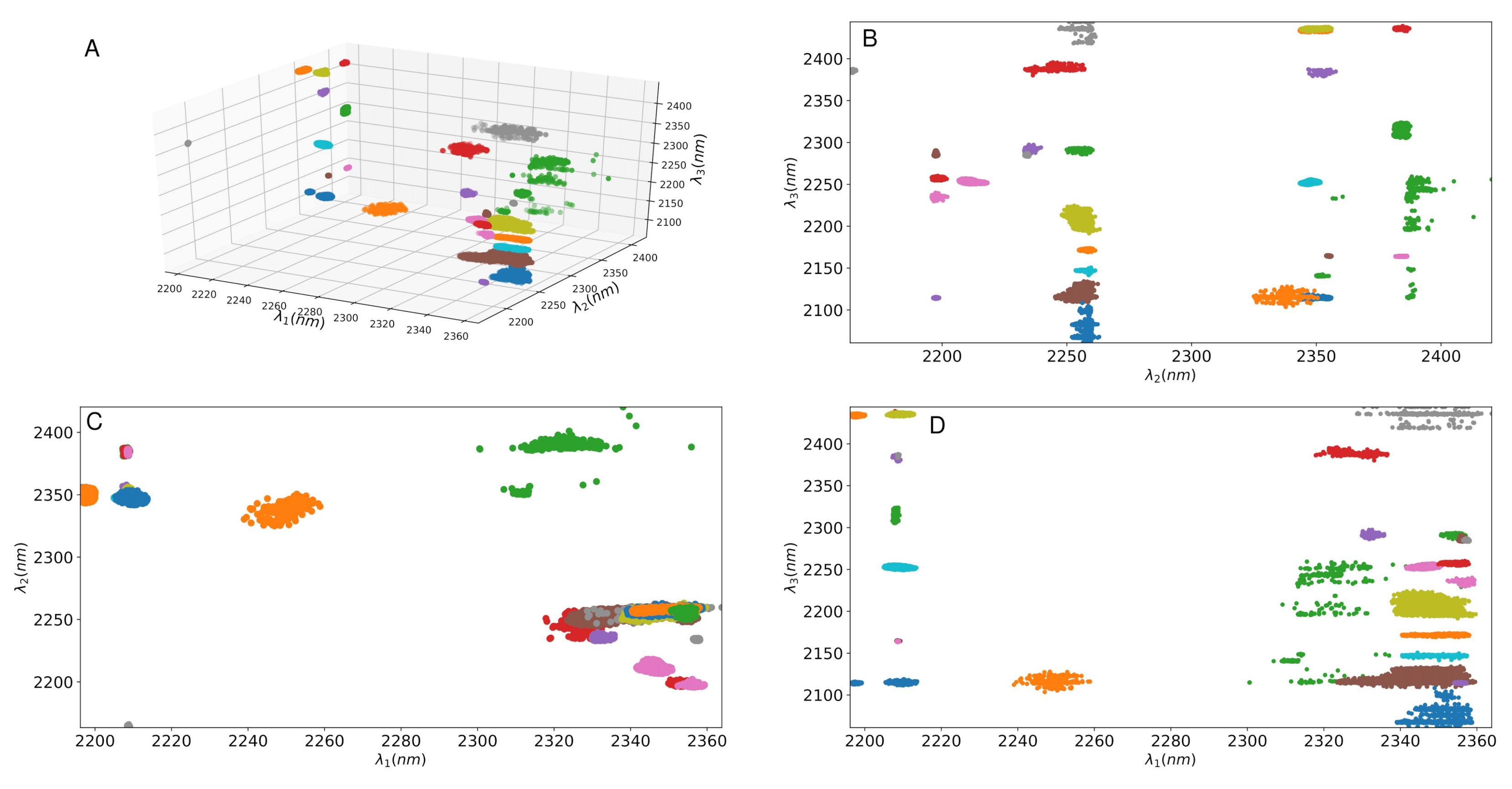
Calculating a median, or mean spectral response (MSR) (users choice) for each cluster allows the mineral assemblage of that cluster to be defined which in turn allows the dataset to be spectrally represented by the total number of clusters rather than the original total number of reflectance spectra. Shown in Figure 2 for illustrative purposes, are the results of applying the workflow to a dense hyperspectral dataset and plotting the 1st, 2nd and 3rd deepest features (top left). The colour of the feature wavelengths shows the cluster assignment as defined by HDBSCAN when the three deepest features are used for clustering.

While definitive clusters are seen in Figure 2 it is often the case that the multiple clusters represent the same mineral assemblages. This effect is due to the depths of those same assemblages being returned in a different order and was also noted by van der Meer et al. [15]. Further similarity measures can be employed to ascertain the potential for merging cluster assignments but this is not pursued here.

3. Data

The reflectance spectra used in this study are from a South Australian geological survey program conducted between 2015–2016 [33,34] and were made publicly available by the Australian National Virtual Core Library through AuScope’s Discovery Portal (http://portal.auscope.org.au/). The Mineral Systems Drilling Program (MSDP) consisted of 14 drill holes for a total of ~8000 m, cored from the surface, aimed at improving the geological understanding of the mineral potential along the margin of a Mesoproterozoic silicic large igneous province in South Australia’s Gawler Craton [35,36,37,38].

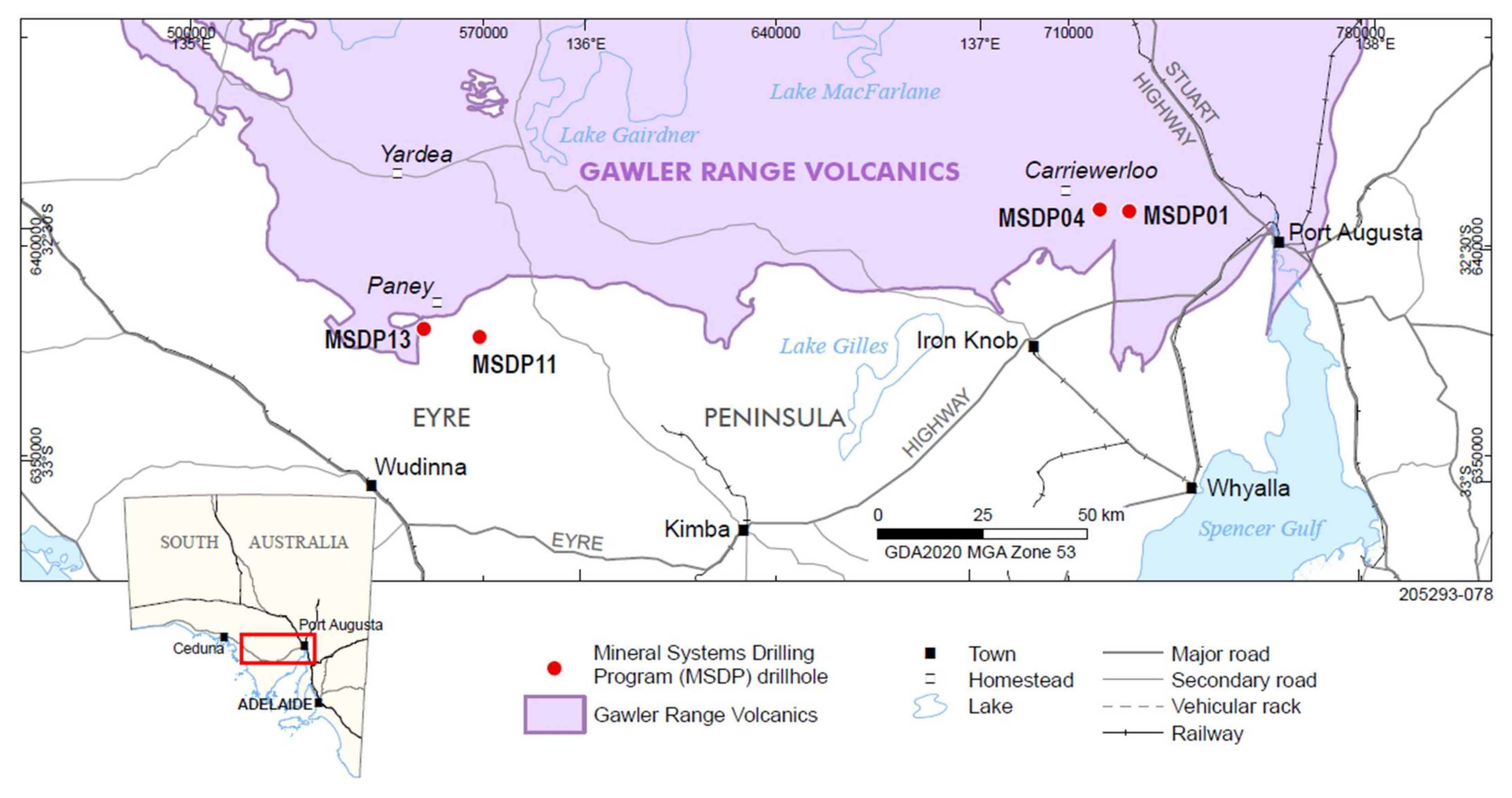
The MSDP series of drill holes provide an ideal case study as they intersect a wide range of lithologies, styles and degrees of alteration, and the program achieved almost complete drill core recovery in all drill holes. All drill cores from the MSDP were scanned with the CSIRO developed HyLogger™ system [8,9]. Results presented herein are from 4 MSDP drill holes (Figure 3), namely MSDP01, 04, 11 and 13.

Each of the MSDP drill cores has an accompanying downhole lithology log, as collected by a field geologist. The lithological summaries are incorporated into the results (Figure 4, Figure 5, Figure 6, Figure 7 and Figure 8) to demonstrate a general correspondence to the lithology, as logged by the geologist, but also highlight mineral assemblages that were not discriminated during the visual drill core logging.

3.1. MSDP01

MSDP01 was cored from the surface to 1116.8 m, with weathering extending to 21.7 m, and intersects highly weathered Quaternary clays, variably weathered Neoproterozoic sandstone, shale and dolomite before intersecting a sequence comprised of felsic and mafic lavas and volcaniclastic units of the Mesoproterozoic Gawler Range Volcanics.

Felsic volcanic intervals are dominated by quartz, plagioclase and K-feldspar with variable sodic plagioclase (albite). Basaltic units within the drill hole consist of a series of lava flows and minor volcaniclastic units. Mineralogy is dominated by feldspar (oligoclase and albite), pyroxene (665.15–964.2 m) and alteration products, chlorite and carbonate. Volcaniclastic units tend to be more altered and at the base of the upper basalt (307–370 m), primary minerals are significantly altered to chlorite and phengite. Very large plagioclase crystals (up to 40 mm) between 142–195 m depth are presumed to have been incorporated into the mafic melt as xenocrysts.

Mineral alteration in MSDP01 ranges in intensity from weak to moderate depending on the unit and is considered to result from regional alteration rather than a mineralizing event. Alteration within felsic volcanic units is characterised by weak selective phengite and weak chlorite (Fe and Fe-Mg compositions), mainly affecting feldspar phenocrysts. Basaltic units contain weak to moderate pervasive chlorite and abundant carbonate-filled vesicles. Very weak pervasive hematite alteration is common within MSDP01 but increases in intensity below 1095 m, associated with a change in lithology.

3.2. MSDP04

Drill hole MSDP04 was cored from the surface to 843.9 m and intersects weathered Quaternary silt, variably weathered trachydacitic lava, basalt, volcaniclastics and rhyolite of the Gawler Range Volcanics, before ending in a fine to coarse-grained dolerite dyke. A high degree of pervasive weathering extends to 12.6 m, after which it decreases and becomes focused along fractures with goethitic and clay fill. Of interest are diverse facies within an overall basaltic unit from 340–437.2 m. Facies include lava, volcaniclastics and mudstone. Approximately 22 m of mafic volcanic breccia overlie mafic lava from 342.75–364.4 m.

Alterations within the drill hole are generally minor and not associated with mineralisation. Weak to moderate intensity hematite–sericite–chlorite alteration zones occur across major unit contacts. Basaltic units contain weak pervasive to patchy chlorite alterations and carbonate-filled amygdales.

3.3. MSDP11

Drillhole MSDP11 was cored from the surface to 498.2 m and intersects Cenozoic alluvial silts and gravels to 26.9 m, before penetrating various basement lithologies. These include porphyrytic felsic intrusives, fine to coarse-grained metadiorite and metagranite, pegmatite, magnetite-rich magnesian skarn and calc-silicate and augen gneiss. Metadioritic units contain common primary hornblende and secondary biotite, grown along foliation plains. Porphyritic felsic units typically have weak selective sericite (muscovitic) and chlorite alterations. Rare disseminations of pyrite, sphalerite, galena and chalcopyrite are evident throughout the drill hole, but are more abundant in the upper felsic porphyritic unit (~50–80 m) and intervals of skarn.

Metadioritic units contain weak to strong pervasive chlorite alterations. Chloritic alterations are mostly intermediate in composition (Fe-Mg), however there are zones dominated by Mg-chlorite (190–208 m; 288–308 m; 445–455 m). Metagranitic units contain weak muscovitic alterations. Close to the skarn, thin metagranite intrusives commonly have magnetite selvages. Zones of skarn are developed within the hole, which host massive magnetite and subordinate hematite and minor pyrite. Skarn mineralogy includes amphibole (tremolite, edenite, actinolite, hornblende), serpentine (lizardite, antigorite), talc, chlorite, pyroxene (diopside), biotite, garnet and quartz, which is characteristic of partly retrogressed magnesian skarn. The augen gneiss at the base of the hole has weak pervasive hematite alterations, weak patchy sericite (muscovitic) alterations and is cut by several intense silica-sericite-pyrite zones that contain elevated Ag values.

3.4. MSDP13

Drill hole MSDP13 was cored from the surface to 502.4 m and intersects 18.1 m of Cenozoic silty sand and gravels before penetrating metasandstone, variably mylonitised calc-silicate and then a visually and chemically distinct metasedimentary unit at the base of the drill hole. Intersected units are highly weathered to 53 m and moderate to weakly weathered to 60.3 m. All lithologies display variable degrees of shearing and deformation. Calc-silicate lithologies are highly strained and have been altered from their original composition to pyroxene (diopside, augite), wollastonite, prehnite, quartz, minor chlorite (Fe > Fe-Mg-rich), epidote and muscovite, trace garnet (andradite) and rare calcite. Quartz boudins are common within calc-silicate units and form in mylonitised zones.

Alteration within the metasandstones is dominated by weak to strong pervasive chlorite (intermediate to Fe-rich compositions), weak to strong silica and weak sericite (dominantly muscovitic). The unit below 492.8 m contains amphibole (actinolite, tremolite), pyroxene (diopside), biotite and weak to strong intensity chlorite (intermediate and Mg-rich compositions) and sericite (muscovite) alteration. Minor Cu and base metal mineralization is associated with narrow breccia zones (433–440 m and ~460 m). Quartz ± chlorite-pyrite veins are common within metasandstones and can be up to 10 mm wide. Veining within the calc-silicate units are dominated by calcite, quartz and chlorite.

4. Results

The results of the proposed workflow to the four-drill cores outlined in the previous section are presented. The wavelength region of interest is maintained as the SWIR from 2050–2450 nm, and the absorptions present in the various hyperspectral datasets mapped downhole. It is noted that samples classed as noise during the clustering phase, or those results with an SCM less than 0.6, are not included in the figures to follow.

In each case the down hole lithology as logged by a geologist is plotted in conjunction with the results. Although the SWIR wavelength region is restricted to absorptions defined by alteration minerals, it is shown that good correspondence can be found between the results and logged lithology. Unless explicitly specified the parameters given in Table 1 are used.

Figure 4, Figure 5, Figure 6 and Figure 7 are all displayed in the same manner which is:

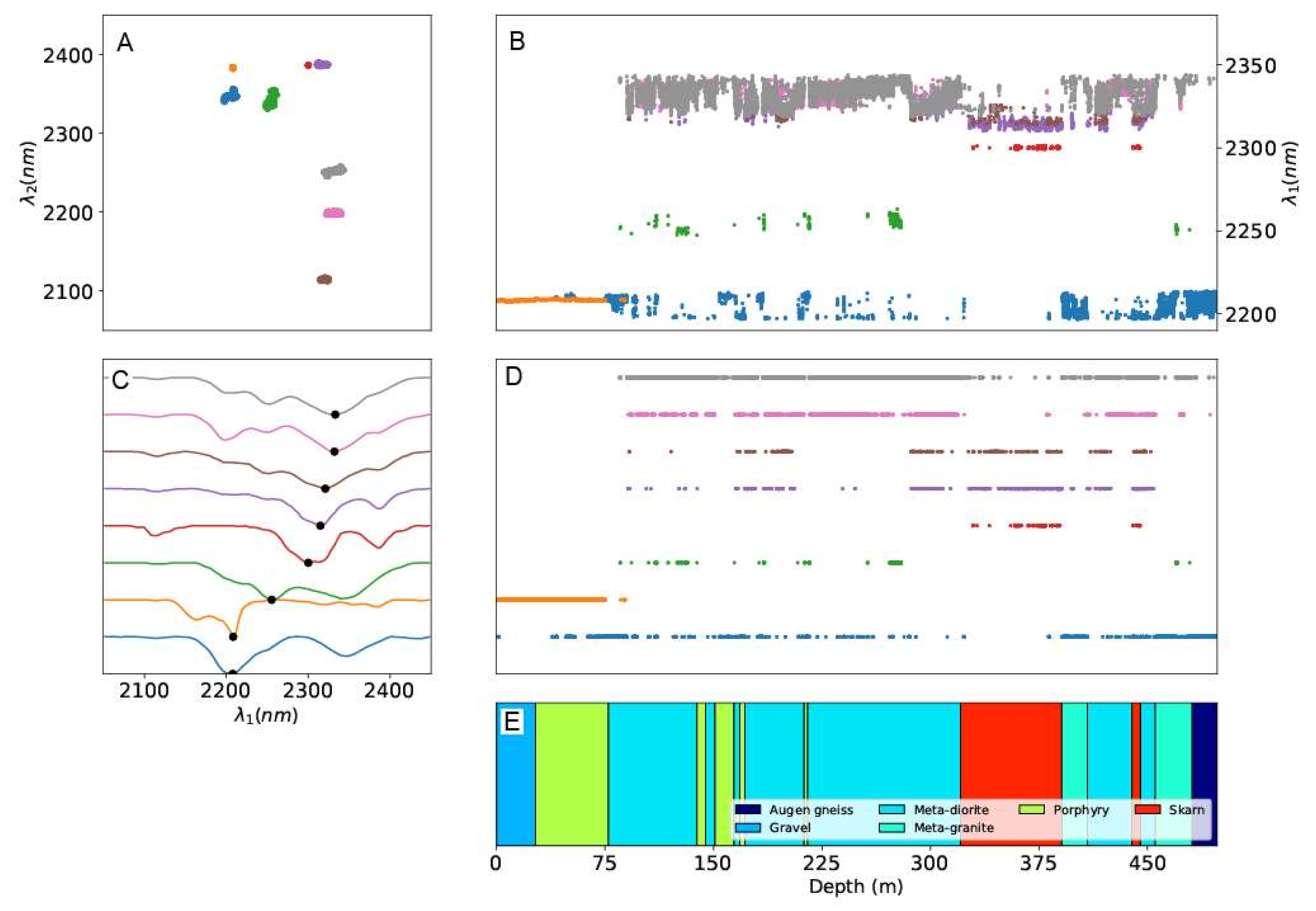
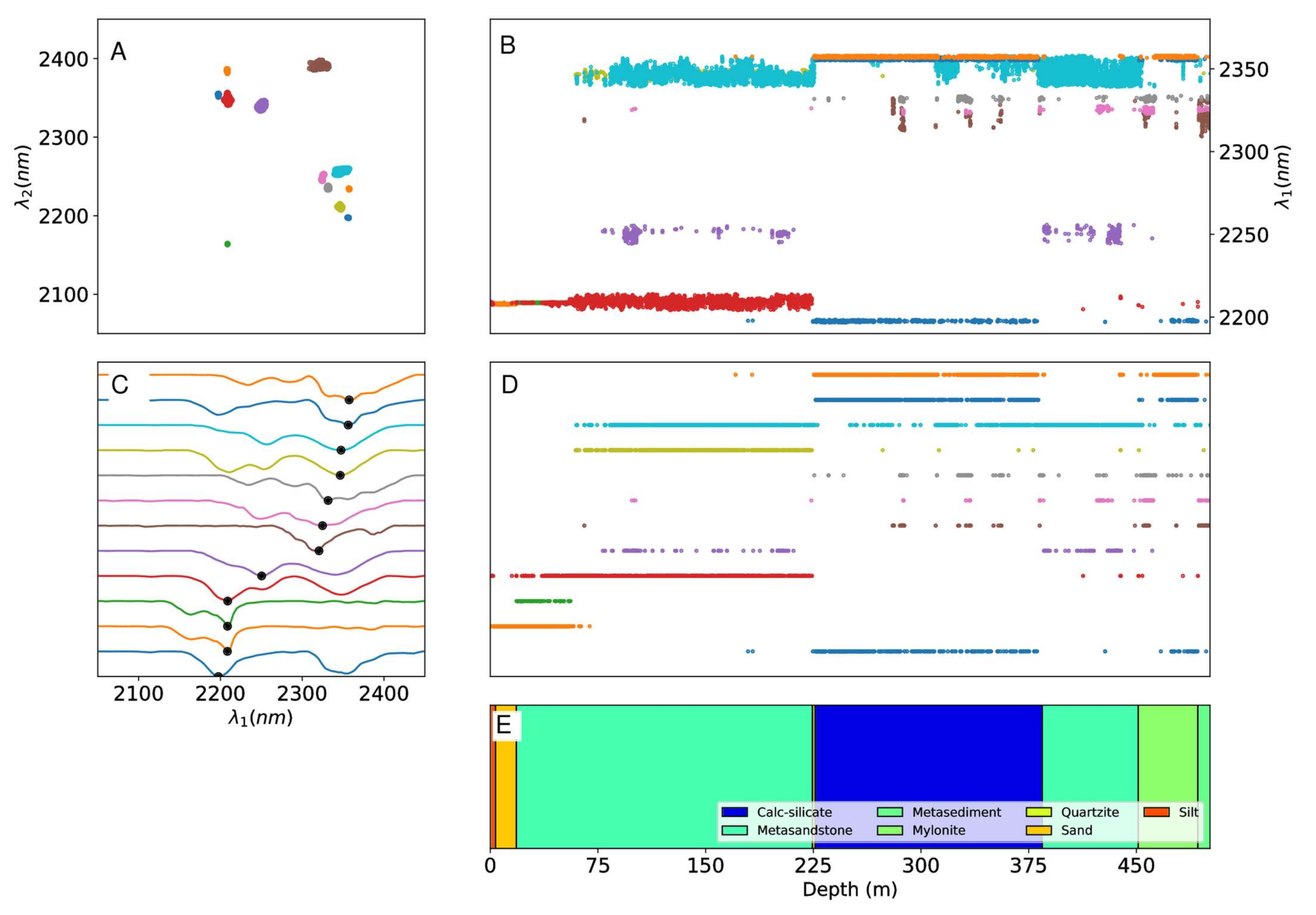
A.

Top-left: Deepest extracted wavelength ${\mathsf{\lambda }}_1$ (x-axis) versus the second deepest extracted wavelength ${\mathsf{\lambda }}_2$ (y-axis) coloured by cluster, as identified by HDBSCAN.

B.

Top-right: Sample depth (x-axis) versus the deepest wavelength (y-axis) coloured by cluster, as identified by HDBSCAN.

C.

Middle-left: Calculated median spectral response (MSR) for a given HDBSCAN with an offset applied to the y-axis for display.

D.

Middle-right: Sample depth (x-axis) coloured by cluster, as identified by HDBSCAN with the same y-axis offset of C.

E.

Bottom-right (E): Depth of logged lithology.

Additionally, it is noted that subplots B, D and E all share the same x-axis, while subplots C and D share the same y-axis, and subplots A and C share the same x-axis. The y-axis of A and B are not shared. The black dots in the C subplots represent the locations of the deepest feature wavelength for that cluster. As noted earlier the MSR of various clusters may be equivalent due to the order of the feature depths however no attempt is made at this stage to merge clusters.

4.1. MSDP01

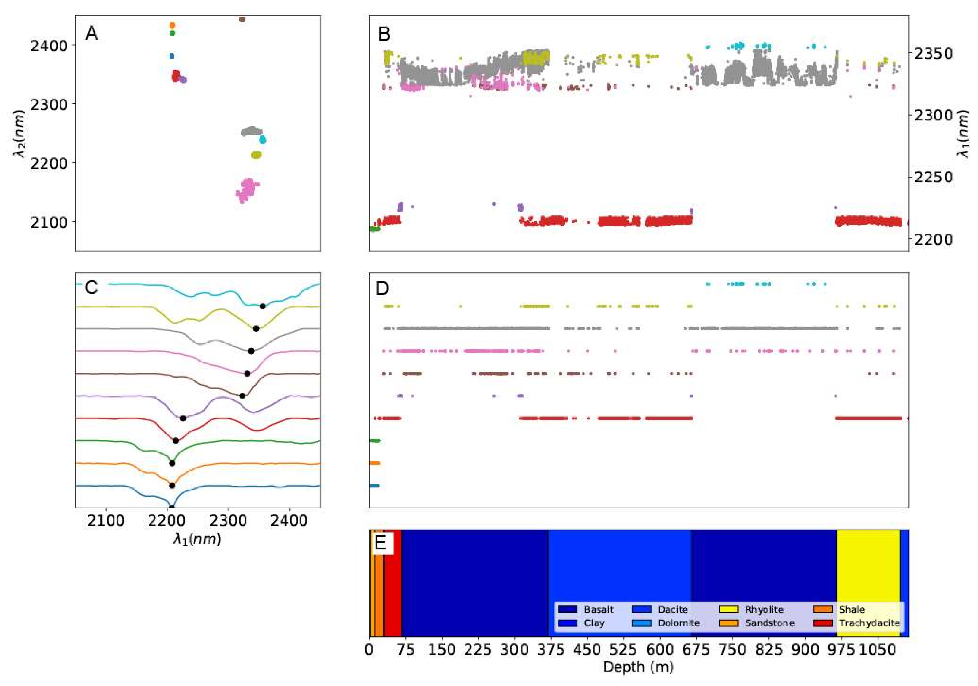
Application to the MSDP01 hyperspectral dataset yields 10 assemblage clusters (Figure 4). It is noted that the “clay” domain in Figure 4E occurs at the very top of the drill hole and as such, is not actually observable in Figure 4E. The spatial distribution of classified features down hole defines domains that generally correspond to the visually logged lithological units. Distinct spectral signatures in the 2050 to 2450 nm wavelength range (three lower-most classes coloured in medium blue, orange and green in Figure 4) are associated with Cenozoic regolith and variably weathered Neoproterozoic sedimentary units overlying Mesoproterozoic volcanic lithologies. The respective reflectance spectra are dominated by kaolin group minerals, as identified by the combined 2160 and 2200 nm absorptions.

In the volcanic lithologies, even though the feature extraction technique is applied to a relatively narrow range of wavelengths, mafic units (e.g., basalt) are distinct from felsic to intermediate units (e.g., rhyolite, trachydacite, dacite). The SWIR reflectance spectra of rhyolite between 950 and 1100 m depth are dominated by white mica.

The occurrence of distinct absorption features and subtle wavelengths shifts of particular features identify some change within similar logged lithologies. For example, the addition of a distinct cluster with absorption features at 2230 nm, 2280 nm, and a very broad feature centred at ~2356 nm, shown in light blue, identifies abundant prehnite in the lower basalts between 680 to 950 m depth as compared to the upper basalt (Figure 4). Prehnite is a common constituent of low grade, regionally metamorphosed rocks, and is restricted to the lower basalt, which suggests either different primary mineral assemblages of the two basalt units or a different degree of metamorphic overprint.

Differences between the logged lithology and the results of the feature extraction are noted and found, for example, in the dacite (369–665 m), where a break in the deepest feature is observed between approximately 400–475 m that has not been identified visually in the lithology log [34]. This may not signify a mineralogical change, warranting a distinct lithology, but identifies a significant change that alerts the user to a region that requires further investigation. Observation of the MSR reflectance spectra in the break indicate the presence of carbonate and/or sheetsilicates (e.g., chlorite, biotite, white mica) as indicated by strong absorptions in the 2320 to 2360 nm wavelength range, and is likely to relate to mineral alteration or an increase in carbonate veining in this region.

4.2. MSDP04

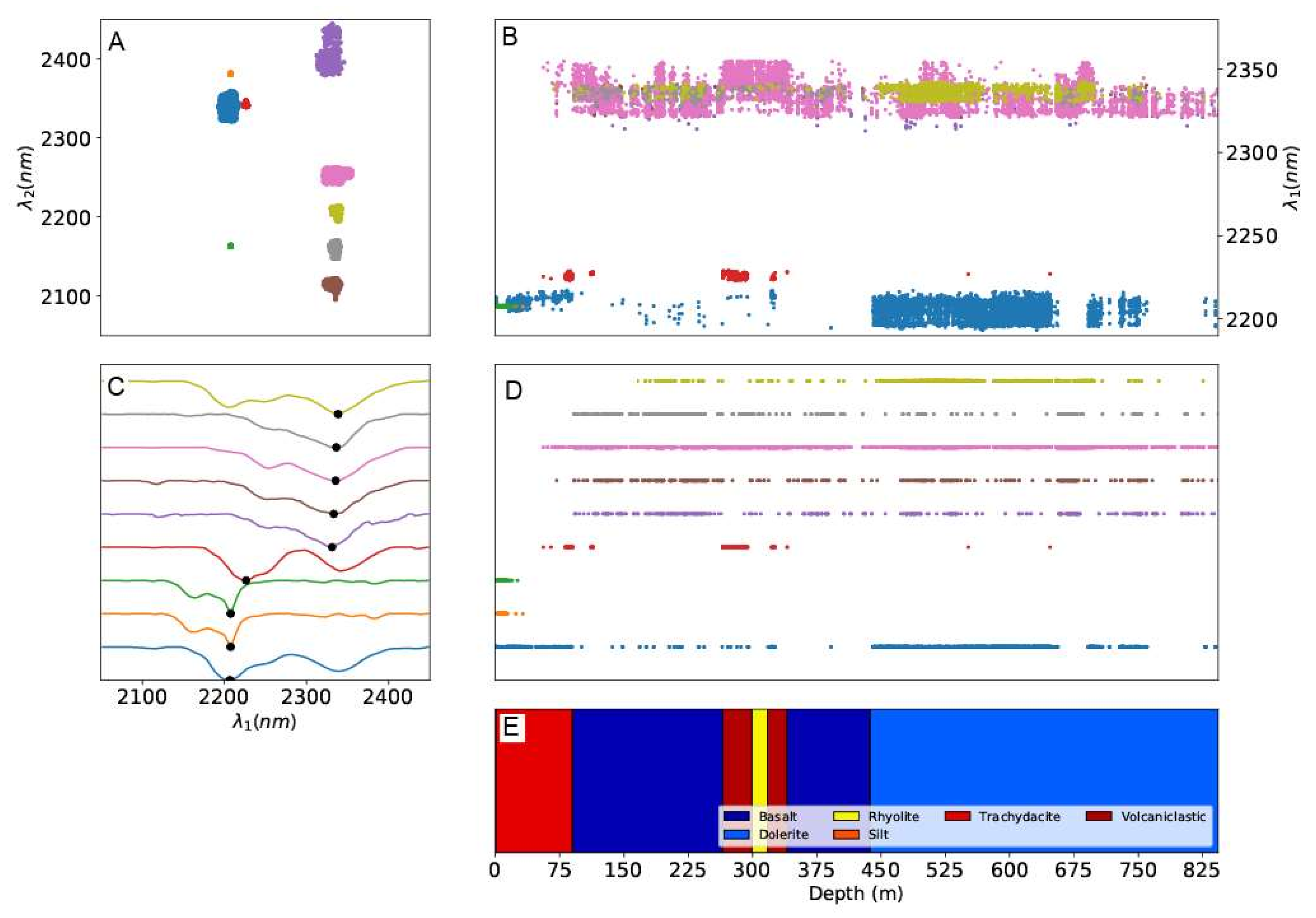
Application to the MSDP04 hyperspectral dataset yields nine assemblage clusters (Figure 5), which, generally identify lithological contacts by breaks in observed features, highlighting several locations of major assemblage change and lithological boundaries. The cluster down hole distributions (Figure 5B) suggest kaolinite (strong absorptions at 2160 and 2200 nm in orange and green reflectance spectra in Figure 5) associated with weathering to 35–40 m. White mica, indicated by the strong 2200 and 2350 nm absorptions, occurs from the top down to approximately 75 m depth, which marks the boundary to the underlying basalt.

The upper level of the basalt unit (90–270 m) is characterised in the results as a region where chlorite represents the main SWIR-active alteration mineral (pink reflectance spectrum in Figure 5C). In some intervals, white mica occurs together with chlorite, as shown by the strong, combined absorptions at around 2200 and 2250 nm (olive green coloured reflectance spectrum in Figure 5C). The rhyolite region (299–317 m) is not immediately apparent but the two volcaniclastic units either side are characterised by strong absorption at ~2225 nm and a shoulder at around 2250 nm (red reflectance spectrum in Figure 5C). The combined 2225 and 2250 nm absorptions potentially indicate that, because both features are very close to each other, the wavelength position of the deepest point of the respective features are influenced by each other. That is, the automatically identified wavelength position of the deepest feature (i.e., 2225 nm) is shifted to longer wavelengths.

The top of the thick dolerite unit (>437 m) is distinguished by the dominance of reflectance spectra showing white mica ± chlorite (2200 and 2350 nm; olive green reflectance spectra in Figure 5C) in the MSR, which is in contrast to the overlying basalts where chlorite is more abundant than white mica. Unlike the lithology log, the results highlight several different zones based on the lack of the mica MSR (light blue reflectance spectra in Figure 5C; between 650–690 m and 760 m onward), suggesting changes in the alteration mineral assemblages, or even subtle lithology changes that were not identified by visual drill core logging. Overall, the SWIR-active mineral assemblages identified by the automated clustering confirm that chlorite and carbonate alteration is much less intense than in drill core MSDP01.

4.3. MSDP11

Automated clustering of the MSDP11 hyperspectral dataset yields eight assemblage clusters (Figure 6). The gravel and upper porphyry units are primarily characterised by the presence of kaolinite (orange MSR: combined 2160 and 2200 nm absorption features), which is prominent from the surface to approximately 75 m and corresponds to an intense weathering overprint on the host lithologies. The meta-diorite unit is effectively resolved, particularly through reflectance spectra showing deepest features at 2200, 2250 and 2350 nm, shown in the pink and grey reflectance spectra in Figure 6C. The difference between these two clusters is that the relative abundance of white mica and chlorite alternates frequently. Sections with higher white mica relative to chlorite abundance show a more prominent 2200 nm absorption feature (i.e., pink reflectance spectra), whereas intervals with stronger chlorite alterations show a more intense 2250 nm absorption feature (i.e., grey reflectance spectra).

Porphyritic units at approximately 150m and meta-granite do not show a strong absorption at 2250 nm, but only strong 2200 and 2350 nm absorptions, suggesting that white mica is the predominant alteration mineral instead of chlorite. This is consistent with the fact that white mica is a typical alteration mineral in the feldspar-rich lithologies such as felsic porphyry and meta-granites. Chlorite alteration is more prominent in mafic rocks.

The skarn unit (320–380 m) is well represented and distinguished by the presence of the reflectance spectra relating to amphibole and/or talc (e.g., red MSR; deepest features at ~2300 nm and ~2380 nm) and is also seen for the smaller skarn unit near 450 m. The presence of talc could indicate a Mg-rich precursor to major parts of the skarn. Amphibole and talc are not identified in any of the clusters in drill cores MSDP01 and MSDP04.

4.4. MSDP13

Application of the automated clustering to the MSDP13 hyperspectral dataset yields 12 assemblage clusters (Figure 7), showing several distinguishable boundaries. The sand/silt (0–18.1 m) units intersected at the top of the drill core can be distinguished through a combination of clustered reflectance spectra dominated by kaolinite (green and orange MSR), and white mica (red MSR in Figure 7C). A shallow but distinct 2250 nm absorption feature in the red reflectance spectra suggests the presence of chlorite up to the surface, which would indicate that the weathering observed in drill core MSDP13 is much less intense than in the other the drill cores, as chlorite is very susceptive to weathering into other Mg/Fe-bearing sheetsilicates, such as vermiculite. However, when comparing the clustering results of drill core MSDP13 based on only the two deepest features with the clustering results based on the three deepest features described further below, the latter classification does not show any 2250 nm absorption features above circa 50 m depths (Figure 8). This suggests that the clustering based on only two features is insufficient to identify the boundary between bedrock and regolith in drill core MSDP13.

The chlorite content increases below circa 75 m depth, as shown by the strong chlorite-related absorption at around 2250 nm in the olive and light blue coloured MSR. The broad wavelength range of the 2200 nm absorption feature in the red MSR displayed in the metasedimentary units (Figure 7A), suggests frequent changes in the composition of the white micas with respect to their Al-content (Table 1). The upper metasandstone unit (60–225 m) is characterised by chlorite and/or white mica content. This contrasts with the lower metasandstone unit (384–451 m), which contains significantly less mica. It is also noted in the lower metasandstone unit that smaller spatial regions are observed in smaller groupings corresponding to the grey, pink and brown MSR with deepest features of 2310, 2320 and 2330 nm, respectively.

The calc-silicate unit (226–384 m) is well defined by white mica (dark blue MSR in Figure 7C) ± chlorite contents (light blue MSR in Figure 7C), very similar to the mylonitised calc-silicate unit below 451 m depth. Similar to the lower basalts in drill core MSDP01, the addition of a distinct cluster with absorption features at 2230 nm, 2280 nm and a very broad feature centred at ~2356 nm shown in orange (Figure 7), identifies abundant prehnite. In contrast to its occurrence in basalt, the prehnite in drill core MSDP13 is often associated with white mica, as shown by the added strong 2200 nm absorption in the top blue MSR.

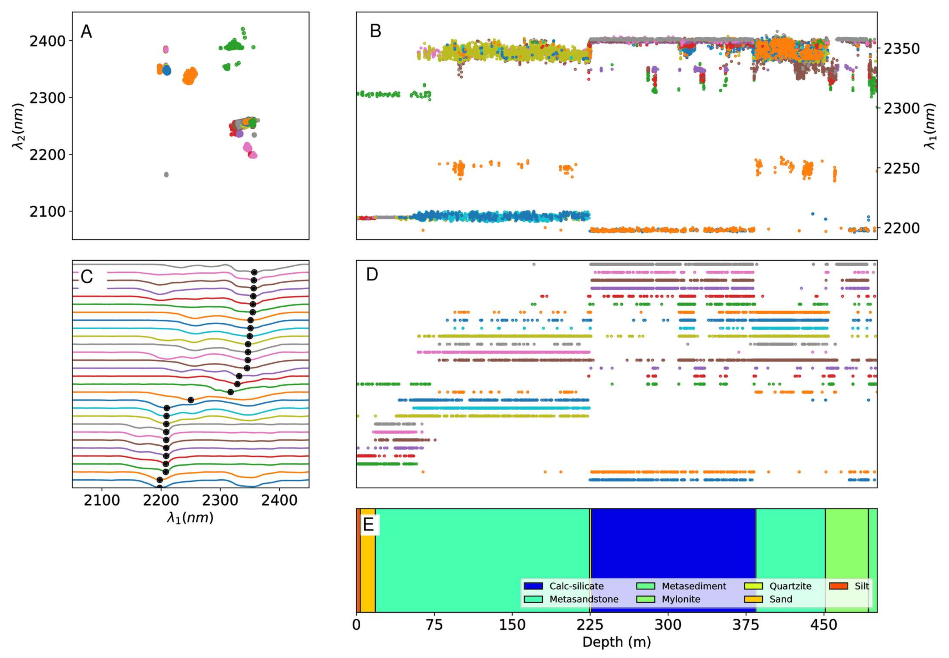
Lastly, Figure 8 demonstrates the results of applying the three deepest features to form clusters, as opposed to only the deepest two as in the previous examples. Due to the larger number of identified clusters, the boundaries of the various regions are more pronounced and subsets of the respective major lithologies are distinguished in more detail. For example, the calcsilicates, visually logged between 225 and 380 m depth, display distinct intervals such as the one between 320 to 330. The latter interval can be discriminated on the base of slight variations with regards to relative intensity of the 2200, 2250 or 2350 nm features, which are not captured when only considering the wavelength position of the two most intense absorption features. It is worth noting that in this case an examination of the reflectance spectra in the individual clusters reveals that many of the MSR are representative of similar assemblages that differ only in the slowly varying deepest wavelength.

5. Conclusions

The workflow outlined here is advantageous when compared to visual drill core logging or manual identification of mineral assemblages on the basis of hyperspectral data for several reasons. Namely, the potential for identifying sections and samples in hyperspectral drill core datasets that might be composed of differing lithology, alterations, weathering overprints and mineral assemblages. The method allows for the simultaneous generation of several products when used in the workflows described.

The scatter plots generated from the combinations of absorption features provide a high-level overview of the potential number of assemblages and minerals present, while the cluster allocations, depending on the dimensionality used, can be used to further refine and spatially locate potential downhole changes. The latter is an additional tool that can be used to confirm or find potential regions of change that may not be readily apparent from only a visual inspection, which can support the decision process about where samples for further analysis should be collected. For example, potentially significant minerals, such as prehnite or talc, which are inherently difficult to identify visually, are readily mapped out. Whilst the here proposed clustering workflow does not necessarily provide answers about the genesis, it highlights compositional differences between visually similar rocks that could entail significant information for lithological classification and even the degree of metamorphic or hydrothermal alteration.

While it was not carried out in this study, it is noted that the outlined workflow is equally applicable to hyperspectral drill core imagery in the same manner as van der Meer et al. [15]. Applying the workflow to drill core imagery allows class maps that are based on the SROI to be produced, which in turn can be used for modal abundance counts. In more traditional methodologies where a specific wavelength is targeted, for example, where a geologist might seek only absorptions between 2300–2350 nm, the resulting singular feature product does not necessarily reveal it may be composed of several assemblages (e.g., white mica, chlorite, calcite; Table 1). Additionally, employing the workflow outlined in this approach still allows us to query the presence of a predefined absorption at a given wavelength, if sought, by searching the returned features for those that are between a constrained wavelength range corresponding to the feature of interest. In this case it is only a search of the returned feature space that is required and not a recalculation, and from which, the depths and feature widths are also available.

Another significant advantage of the feature extraction method described here, is that it is not overly computationally expensive and it is relatively fast. All the examples used in this study were calculated on a standard laptop and ran in a few minutes per drill core. In general, this meant performing data input and output, hull corrections, feature extraction and clustering of 70,000 reflectance spectra (mean).

Applying the proposed method with no a-priori assumptions about the composition of the mineral assemblages provides a means of generating an informative overview of the dataset that is not biased or constrained by preconceptions. In an active exploration setting where spectral data are collected in the field, the ability to identify regions that might benefit from increased or decreased laboratory analysis can be made and have the potential to reduce overall lab expenditure, or to focus on more economic target areas. Additionally, the ability to define potential boundaries, and regions of little to no variability, within the drill core can guide the geologist to those regions that may be most representative of lithological and/or alteration changes.

References

- Burley, L.L.; Barnes, S.J.; Laukamp, C.; Mole, D.R.; Le Vaillant, M.; Fiorentini, M.L. Rapid mineralogical and geochemical characterisation of the Fisher East nickel sulphide prospects, Western Australia, using hyperspectral and pXRF data. Ore Geol. Rev. 2017, 90, 371–387. [Google Scholar] [CrossRef]
- Gordon, G.; McAvaney, S.; Wade, C. Spectral characteristics of the Gawler Range Volcanics in drill core Myall Creek RC1. Aust. J. Earth Sci. 2016, 63, 973–986. [Google Scholar]
- Lampinen, H.M.; Laukamp, C.; Occhipinti, S.A.; Hardy, L. Mineral footprints of the Paleoproterozoic sediment-hosted Abra Pb-Zn-Cu-Au deposit Capricorn Orogen, Western Australia. Ore Geol. Rev. 2019, 104, 436–461. [Google Scholar] [CrossRef]
- Mauger, A.J.; Ehrig, K.; Kontonikas-Charos, A.; Ciobanu, C.L.; Cook, N.J.; Kamenetsky, V.S. Alteration at the Olympic Dam IOCG–U deposit: Insights into distal to proximal feldspar and phyllosilicate chemistry from infrared reflectance spectroscopy. Aust. J. Earth Sci. 2016, 63, 959–972. [Google Scholar] [CrossRef]
- Kruse, F.A. Identification and mapping of minerals in drill core using hyperspectral image analysis of infrared reflectance spectra. Int. J. Remote Sens. 1996, 17, 1623–1632. [Google Scholar] [CrossRef]
- Sonntag, I.; Laukamp, C.; Hagemann, S.G. Low potassium hydrothermal alteration in low sulfidation epithermal systems as detected by IRS and XRD: An example from the Co–O mine, Eastern Mindanao, Philippines. Ore Geol. Rev. 2012, 45, 47–60. [Google Scholar] [CrossRef]
- Yang, K.; Lian, C.; Huntington, J.F.; Peng, Q.; Wang, Q. Infrared spectral reflectance characterization of the hydrothermal alteration at the Tuwu Cu–Au deposit, Xinjiang, China. Miner. Depos. 2005, 40, 324–336. [Google Scholar] [CrossRef]
- Huntington, J.; Whitbourn, L.; Mason, P.; Berman, M.; Schodlok, M.C. HyLogging—Voluminous industrial-scale reflectance spectroscopy of the Earth’s subsurface. In Proceedings of the ASD and IEEE GRS; Art, Science and Applications of Reflectance Spectroscopy Symposium, Boulder, CO, USA, 23–25 February 2010; Volume 2, p. 14. [Google Scholar]
- Schodlok, M.C.; Whitbourn, L.; Huntington, J.; Mason, P.; Green, A.; Berman, M.; Coward, D.; Connor, P.; Wright, W.; Jolivet, M. HyLogger-3, a visible to shortwave and thermal infrared reflectance spectrometer system for drill core logging: Functional description. Aust. J. Earth Sci. 2016, 63, 929–940. [Google Scholar]
- Harraden, C.L.; Berry, R.; Lett, J. Proposed methodology for utilising automated core logging technology to extract geotechnical index parameters. In Proceedings of the International Geometallurgy Conference, Perth, Australia, 15–17 June 2016; pp. 15–16. [Google Scholar]
- Berman, M.; Bischof, L.; Huntington, J. Algorithms and software for the automated identification of minerals using field spectra or hyperspectral imagery. In Proceedings of the 13th International Conference on Applied Geologic Remote Sensing, Vancouver, BC, Canada, 1–3 March 1999; Volume 1, pp. 222–232. [Google Scholar]
- Cudahy, T.; Jones, M.; Thomas, M.; Laukamp, C.; Caccetta, M.; Hewson, R.; Verrall, M.; Hacket, A.; Rodger, A. Mineral Mapping Queensland: Iron Oxide Copper Gold (IOCG) Mineral System Case History, Starra, Mount Isa Inlier; Australasian Institute of Mining and Metallurgy: Gold Coast, Queensland, Australia, 2008; pp. 153–160. [Google Scholar]
- Laukamp, C.; Cacetta, M.; Chia, J.; Cudahy, T.; Gessner, G.; Haest, M.; Liu, Y.C.; Ong, C.; Rodger, A. The uses, abuses and opportunities for hyperspectral technologies and derived geoscience information. AIG Bull. 2010, 51, 73–76. [Google Scholar]
- Bakker, W.; van Ruitenbeek, F.J.A.; van der Werff, H.M.A. Hyperspectral image mapping by automatic color coding of absorption features. In Proceedings of the 7th EARSEL Workshop of the Special Interest Group in Imaging Spectroscopy, Edinburgh, UK, 11–13 April 2011; pp. 56–57. [Google Scholar]
- van der Meer, F.; Kopačková, V.; Koucká, L.; van der Werff, H.M.A.; van Ruitenbeek, F.J.A.; Bakker, W.H. Wavelength feature mapping as a proxy to mineral chemistry for investigating geologic systems: An example from the Rodalquilar epithermal system. Int. J. Appl. Earth Obs. Geoinf. 2018, 64, 237–248. [Google Scholar] [CrossRef]
- van Ruitenbeek, F.J.A.; Bakker, W.H.; van der Werff, H.M.A.; Zegers, T.E.; Oosthoek, J.H.P.; Omer, Z.A.; Marsh, S.H.; van der Meer, F.D. Mapping the wavelength position of deepest absorption features to explore mineral diversity in hyperspectral images. Planet. Space Sci. 2014, 101, 108–117. [Google Scholar] [CrossRef]
- Laukamp, C.; Cudahy, T.; Thomas, M.; Jones, M.; Cleverley, J.S.; Oliver, N.H.S. Hydrothermal mineral alteration patterns in the Mount Isa Inlier revealed by airborne hyperspectral data. Aust. J. Earth Sci. 2011, 58, 917–936. [Google Scholar]
- Virtanen, P.; Gommers, R.; Oliphant, T.E.; Haberland, M.; Reddy, T.; Cournapeau, D.; Burovski, E.; Peterson, P.; Weckesser, W.; Bright, J. SciPy 1.0: Fundamental Algorithms for Scientific Computing in Python. Nature Methods 2020, 17, 261–272. [Google Scholar] [CrossRef] [PubMed] [Green Version]
- Millman, K.J.; Aivazis, M. Python for scientists and engineers. Comput. Sci. Eng. 2011, 13, 9–12. [Google Scholar] [CrossRef] [Green Version]
- Oliphant, T.E. Python for scientific computing. Comput. Sci. Eng. 2007, 9, 10–20. [Google Scholar] [CrossRef] [Green Version]
- Rodger, A.; Laukamp, C.; Haest, M.; Cudahy, T. A simple quadratic method of absorption feature wavelength estimation in continuum removed spectra. Remote Sens. Environ. 2012, 118, 273–283. [Google Scholar] [CrossRef]
- Frost, R.L.; Johansson, U. Combination bands in the infrared spectroscopy of kaolins—a drift spectroscopic study. Clays Clay Miner. 1998, 46, 466–477. [Google Scholar] [CrossRef]
- Vedder, W.; McDonald, R.S. Vibrations of the OH Ions in Muscovite. J. Chem. Phys. 1963, 38, 1583–1590. [Google Scholar] [CrossRef]
- McLeod, R.L.; Gabell, A.R.; Green, A.A.; Gardavsky, V. Chlorite infrared spectral data as proximity indicators of volcanogenic massive sulphide mineralisation. In Proceedings of the Pacific Rim Congress, Gold Coast, Australia, 26–29 August 1987. [Google Scholar]
- Bishop, J.L.; Lane, M.D.; Dyar, M.D.; Brown, A.J. Reflectance and emission spectroscopy study of four groups of phyllosilicates: Smectites, kaolinite-serpentines, chlorites and micas. Clay Miner. 2008, 43, 35–54. [Google Scholar]
- LeGras, M.; Laukamp, C.; Lau, I.C.; Mason, P. NVCL Spectral Reference Library Phyllosilicates Part 2: Micas; CSIRO Report Number EP183095; CSIRO: Canberra, Australia, 2018. [Google Scholar]
- Lypaczewski, P.; Rivard, B. Estimating the Mg# and AlVI content of biotite and chlorite from shortwave infrared reflectance spectroscopy: Predictive equations and recommendations for their use. Int. J. Appl. Earth Obs. Geoinf. 2018, 68, 116–126. [Google Scholar]
- Laukamp, C.; Termin, K.A.; Pejcic, B.; Haest, M.; Cudahy, T. Vibrational spectroscopy of calcic amphiboles—applications for exploration and mining. Eur. J. Mineral. 2012, 24, 863–878. [Google Scholar] [CrossRef]
- Gaffey, S.J. Spectral reflectance of-carbonate minerals in the visible and near infrared (0.35–2.55 microns): Calcite, aragonite, and dolomite. Am. Mineral. 1986, 71, 151–162. [Google Scholar]
- Clark, R.N.; Roush, T.L. Reflectance spectroscopy: Quantitative analysis techniques for remote sensing applications. J. Geophys. Res. Solid Earth 1984, 89, 6329–6340. [Google Scholar] [CrossRef]
- McInnes, L.; Healy, J.; Astels, S. hdbscan: Hierarchical density based clustering. J. Open Source Softw. 2017, 2, 205. [Google Scholar] [CrossRef]
- Schubert, E.; Sander, J.; Ester, M.; Kriegel, H.P.; Xu, X. DBSCAN revisited, revisited: Why and how you should (still) use DBSCAN. ACM Trans. Database Syst. TODS 2017, 42, 1–21. [Google Scholar] [CrossRef]
- Fabris, A. Geological outcomes of the Mineral Systems Drilling Program along the southern Gawler Ranges. MESA J. 2017, 85, 12–23. [Google Scholar]
- Fabris, A.; Tylkowski, L.; Brennan, J.; Flint, R.B.; Ogilvie, A.; McAvaney, S.; Werner, M.; Pawley, M.; Krapf, C.; Burtt, A.C. Mineral Systems Drilling Program in the Southern Gawler Ranges, South Australia; Deep Exploration Technologies Cooperative Research Centre: Adelaide Airport, Australia, 2017. [Google Scholar]
- Allen, S.R.; Simpson, C.J.; McPhie, J.; Daly, S.J. Stratigraphy, distribution and geochemistry of widespread felsic volcanic units in the Mesoproterozoic Gawler Range Volcanics, South Australia. Aust. J. Earth Sci. 2003, 50, 97–112. [Google Scholar] [CrossRef]
- Blissett, A.H. Gawler range volcanics. Geol. S. Aust. Precambrian 1993, 1, 107–124. [Google Scholar]
- Hand, M.; Reid, A.; Jagodzinski, L. Tectonic framework and evolution of the Gawler Craton, Southern Australia. Econ. Geol. 2007, 102, 1377–1395. [Google Scholar] [CrossRef]
- Reid, A.J.; Hand, M. Mesoarchean to Mesoproterozoic evolution of the southern Gawler Craton, South Australia. Episodes J. Int. Geosci. 2012, 35, 216–225. [Google Scholar] [CrossRef] [Green Version]
Figure 1.
A reflectance spectrum (blue) and the corresponding hull quotient (orange) and (green) after background removal. The location of 5 different features are shown located at the red markers and the depth of the two largest features shown by the black vertical lines. It is noted that for very small depths the vertical line is not distinguisable.
Figure 2.
Extracting the deepest, second and third deepest absoprtion features in the 2050–2450 nm spectral region of a spectral dataset and clustering yields the results shown in the (A). The different colours in this case are to simply highlight the different clusters and so the reader may see how they are located in the 3D space. Plotting the various feature combinations against each other demonstrates the spectral distribution of the extracted features. (C) is the deepest versus second deepest feature wavelengths, (B) is the second versus third deepest feature wavelngths and (D) is the first versus third deepest.
Figure 3.
Location of drill holes MSDP01, 04, 11 and 13 for the Mineral Systems Drilling Program, southern Gawler Ranges, South Australia. Coordinate system is Geocentric Datum of Australia (GDA) 2020, Map Grid Australia (MGA) Zone 53.
Figure 4.
The 1st and 2nd deepest wavelength location of the extracted features in the 2050–2450 nm spectral region of the MSDP01 dataset (A), the down hole deepest feature as a function of hole depth (B). (C) shows the calculated MSR assemblages for each of the clusters in the top-left while the (D) plot shows the down hole distribution of those assemblages and (E) is the geologists logged litholgy. See the text included in the Results section for a more detailed explanation of the individual plots.
Figure 5.
The 1st and 2nd deepest wavelength location of the extracted features in the 2050–2450 nm spectral region of the MSDP04 dataset (A), the down hole deepest feature as a function of hole depth (B). (C) shows the calculated MSR assemblages for each of the clusters in the top-left while the (D) plot shows the down hole distribution of those assemblages and (E) is the geologists logged litholgy. See the text included in the Results Section for a more detailed explanation of the individual plots.
Figure 6.
The 1st and 2nd deepest wavelength location of the extracted features in the 2050–2450 nm spectral region of the MSDP11 dataset (A), the down hole deepest feature as a function of hole depth (B). (C) shows the calculated MSR assemblages for each of the clusters in the top-left while the (D) plot shows the down hole distribution of those assemblages and (E) is the geologists logged litholgy. See the text included in the Results Section for a more detailed explanation of the individual plots.
Figure 7.
The 1st and 2nd deepest wavelength location of the extracted features in the 2050–2450 nm spectral region of the MSDP13 dataset (A), the down hole deepest feature as a function of hole depth (B). (C) shows the calculated MSR assemblages for each of the clusters in the top-left while the (D) plot shows the down hole distribution of those assemblages and (E) is the geologists logged litholgy. See the text included in the Results Section for a more detailed explanation of the individual plots.
Figure 8.
Using a hierarchical density-based clustering (HDBSCAN) clustering dimension of 3. The 1st and 2nd deepest wavelength location of the extracted features in the 2050–2450 nm spectral region of the MSDP13 dataset (A) and the down hole deepest feature as a function of hole depth (B). The (C) plot shows the calculated MSR assemblages for each of the clusters in the top-left while the (D) plot shows the down hole distribution of those assemblages and the (E) plot is the geologist’s logged litholgy. While a greater number of assemblages are observed and could be combined, the distribution plot middle-right reveals a greater amount of detail when compared to the geologist’s logged lithology bottom-right.