
Problems of Estimating the Resources of Accompanying Elements: A Case Study from the Cu-Ag Rudna Deposit (Legnica-Głogów Copper District, Poland)

 ,
,  ,
,  and
and
Abstract
:1. Introduction
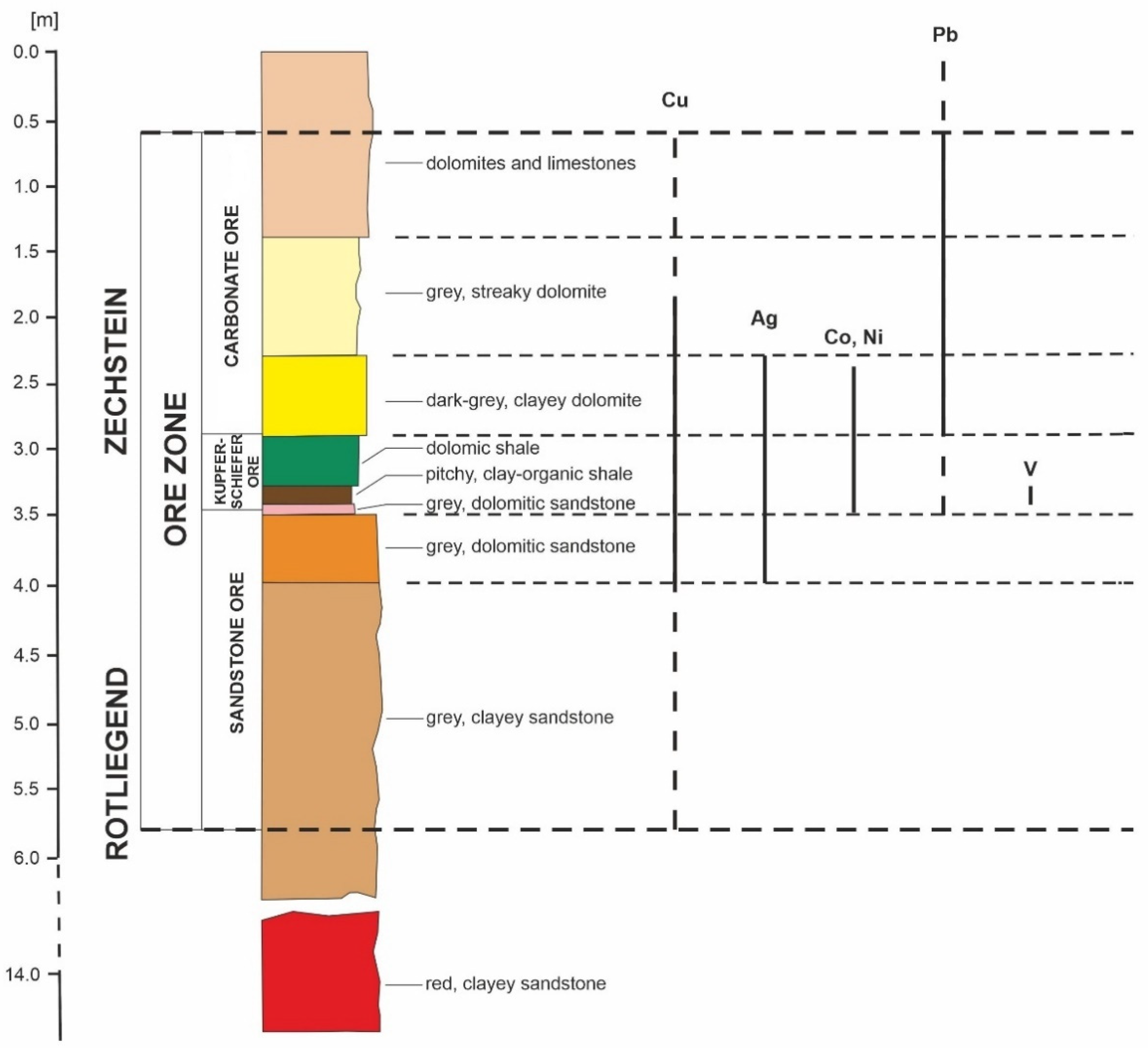
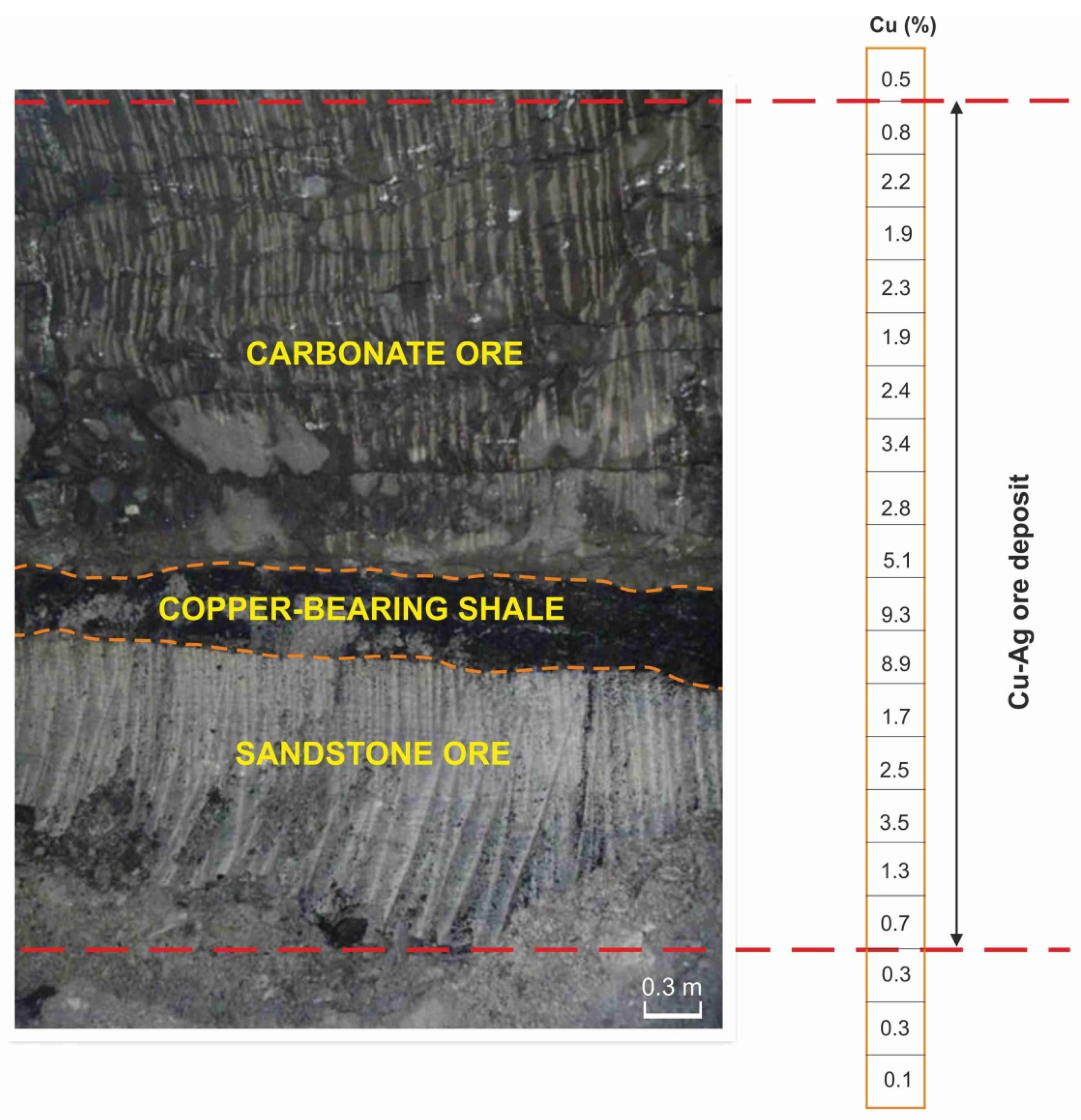
2. Geology
2.1. Geological Setting
2.2. Characteristics of the Studied Accompanying Elements

3. Materials and Methods
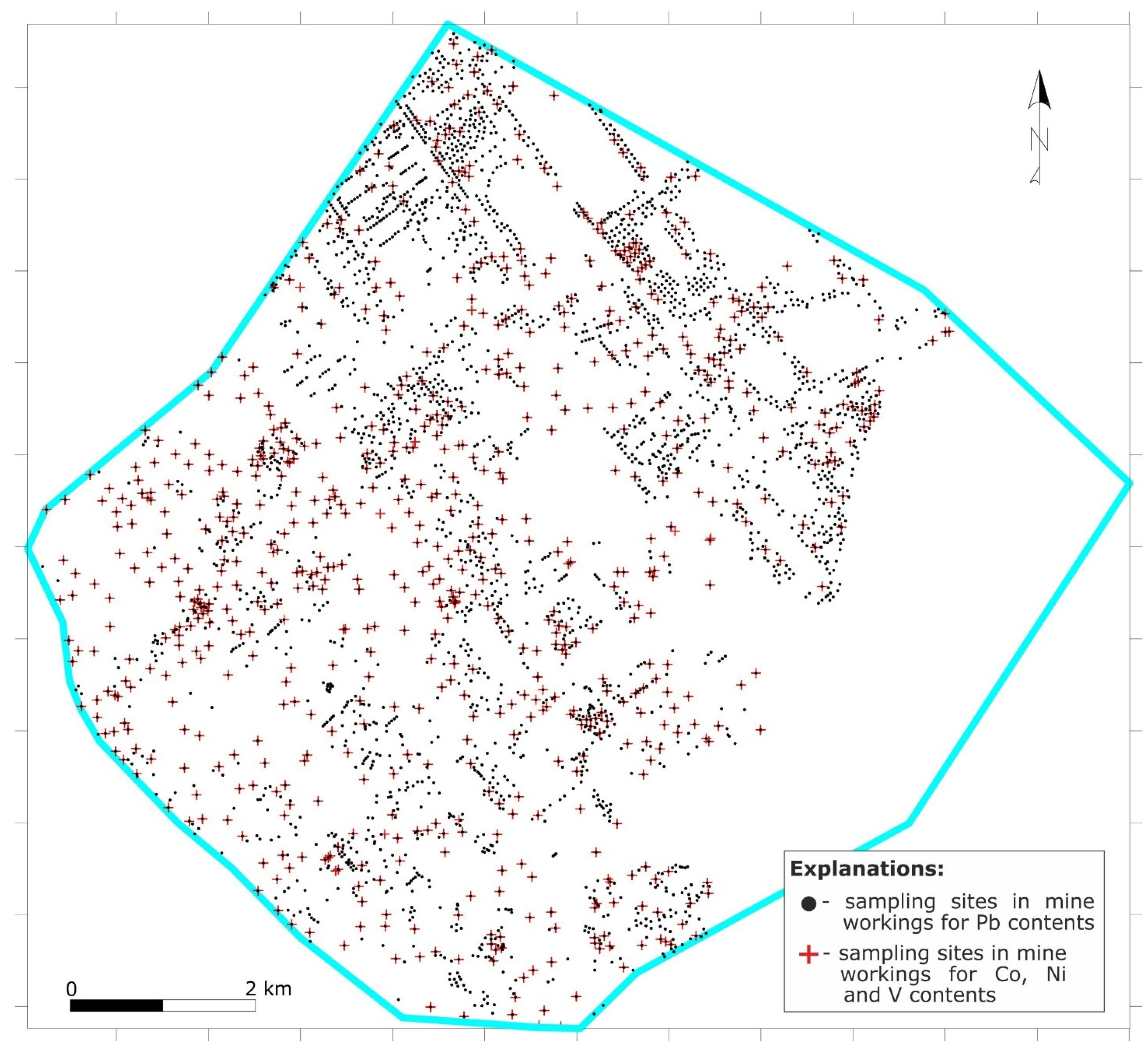
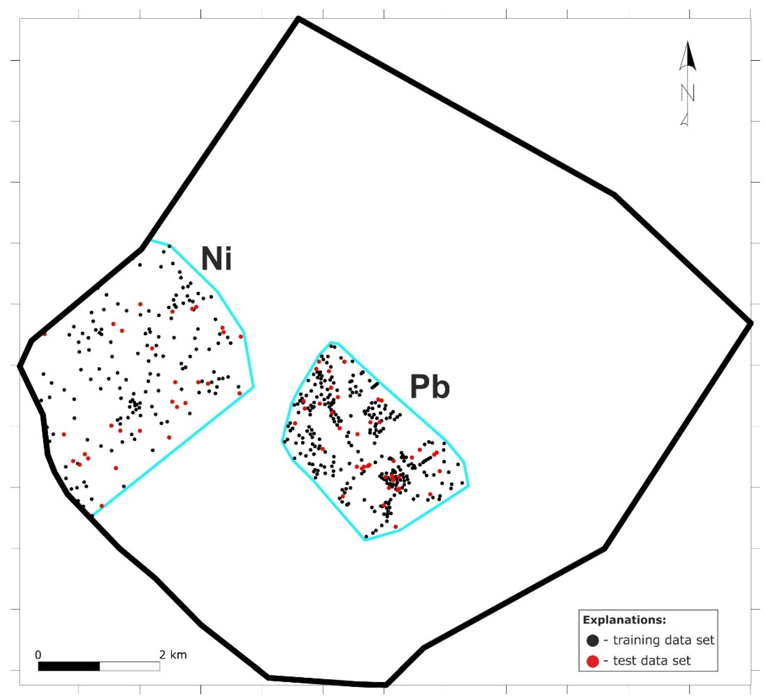
3.1. Sampling of the Deposit in Mine Workings
3.2. Methods
4. Results
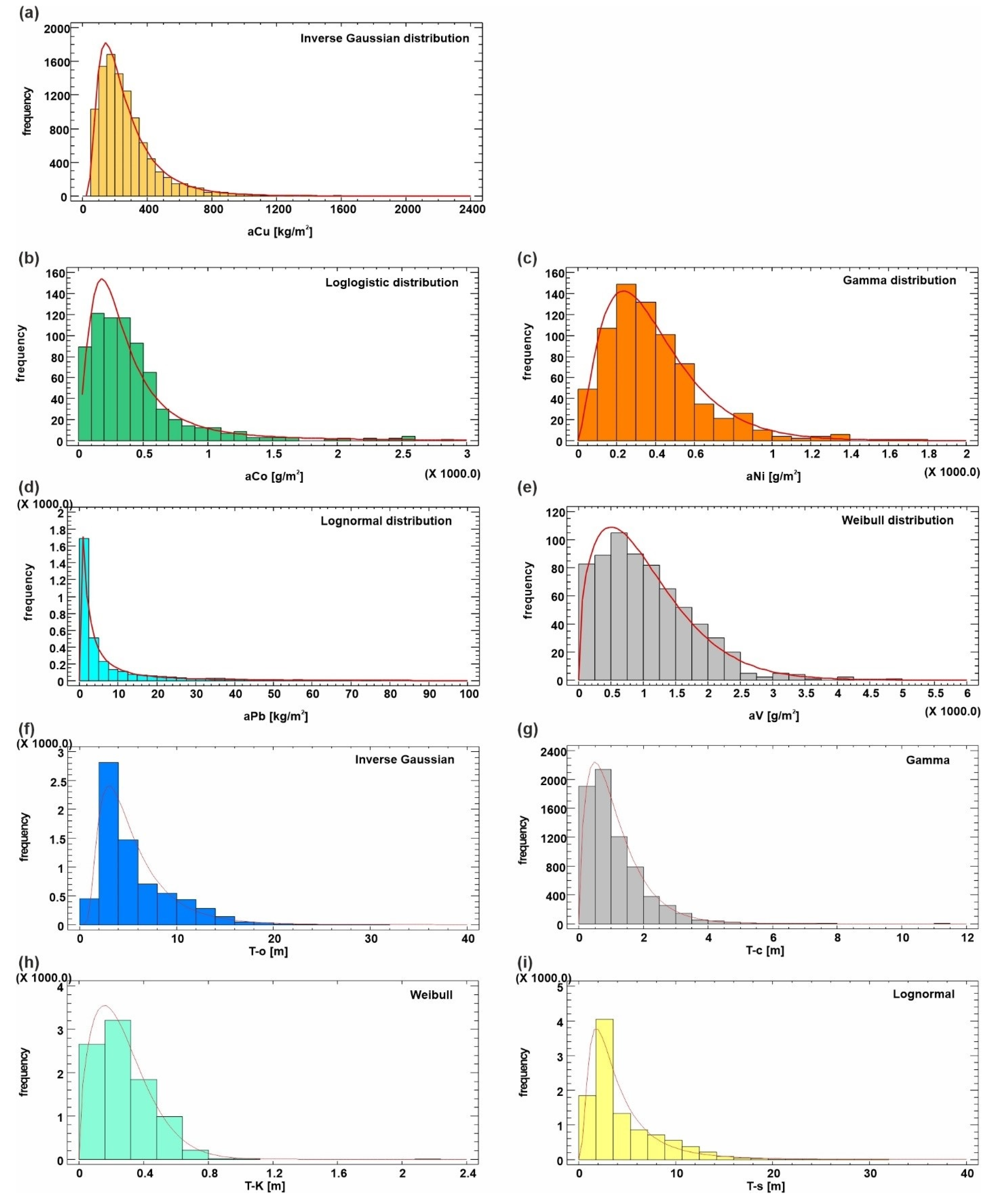
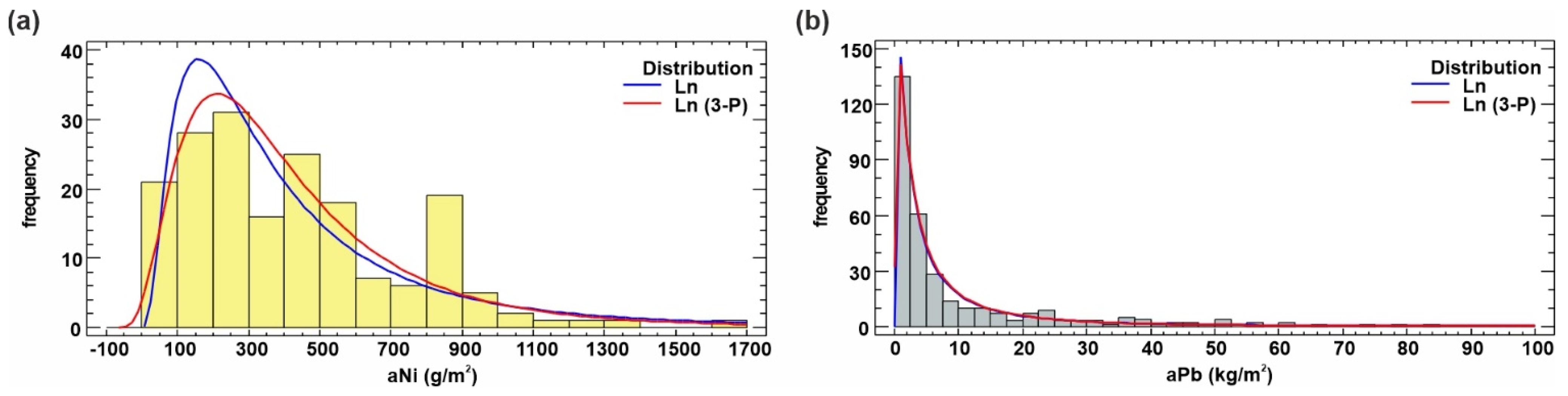
4.1. Statistical Features of the Abundance of Copper and Accompanying Elements
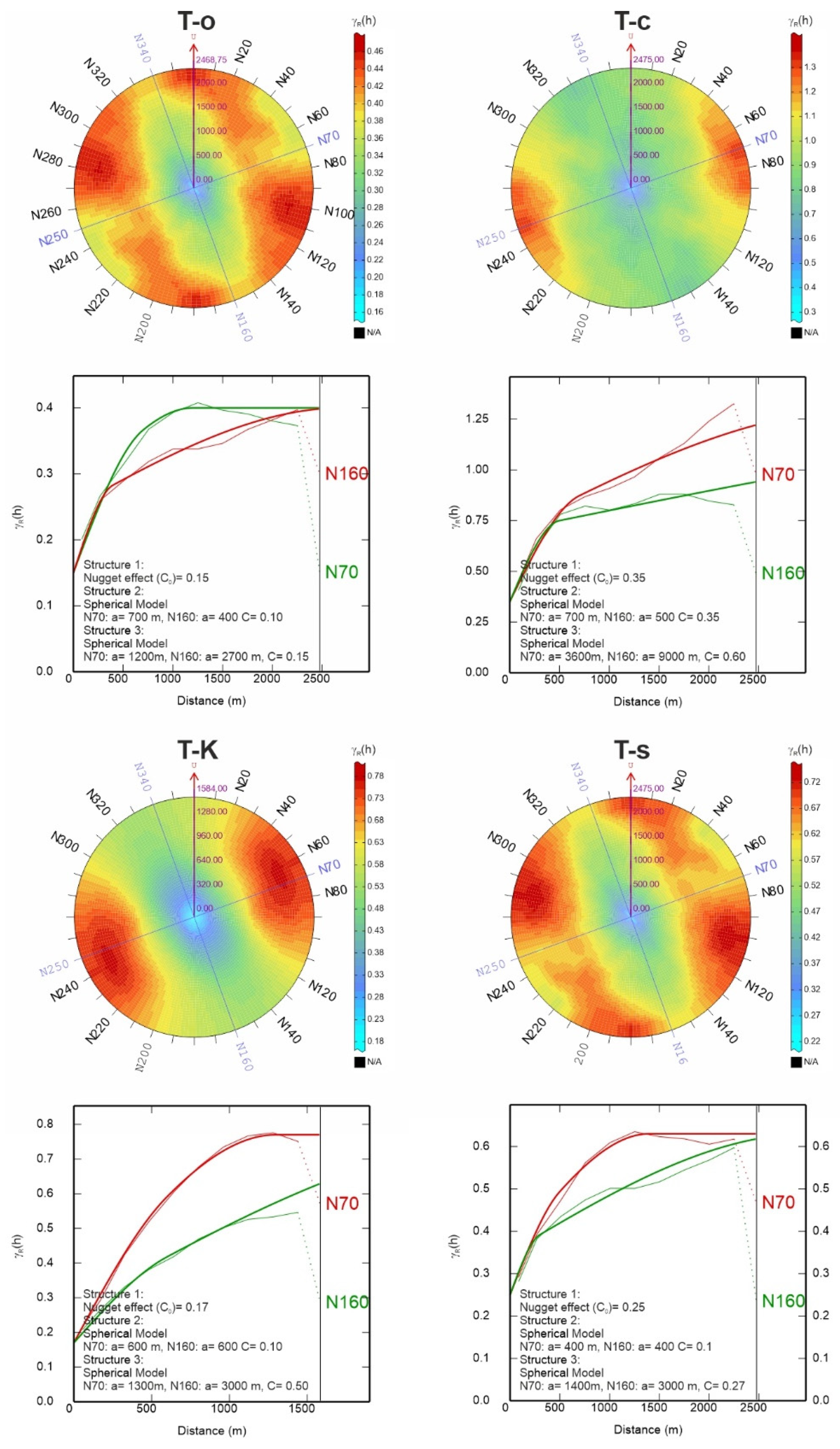
4.2. Variography
4.3. Accuracy of the Point Prediction of Ni and Pb Abundance
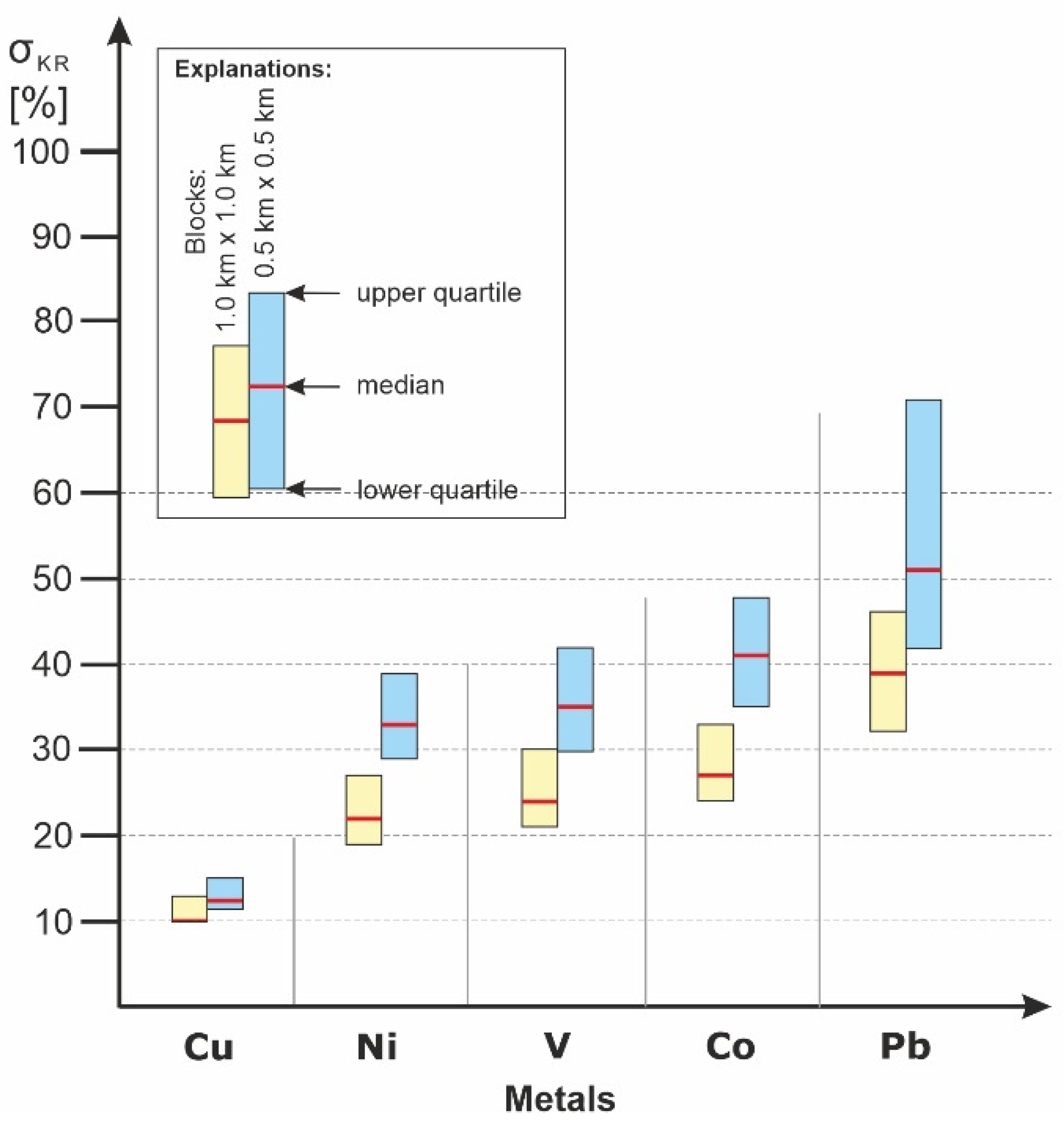
4.4. Accuracy of Estimation of Accompanying Elements in Deposit Blocks
5. Summary and Discussion
6. Conclusions
Author Contributions
Funding
Conflicts of Interest
References
- Newman, P.; Meader, N.; Klapwijk, P.; Liang, J.; Chou, E.; Gao, Y.; Barot, H.; Furuno, A.; Rey, F.; Yau, S.; et al. Metals Focus. World Silver Survey; The Silver Institute and Metals Focus: Washington, DC, USA, 2021. [Google Scholar]
- Malon, A.; Tymiński, M.; Mikulski, M.Z.; Oszczepalski, S. Surowce metaliczne. In Bilans Zasobów Złóż Kopalin w Polsce; Szuflicki, M., Malon, A., Tymiński, M., Eds.; Państwowy Instytut Geologiczny—Państwowy Instytut Badawczy: Warszawa, Poland, 2020. [Google Scholar]
- Banaś, M.; Kijewski, P.; Salamon, W.; Pieczonka, J.; Piestrzyński, A. Monografia KGHM Polska Miedź S.A.; Pierwiastki Towarzyszące w złożu rud miedzi; KGHM Cuprum Sp. z.o.o. CBR: Wrocław, Poland, 2007; pp. 214–228. [Google Scholar]
- Chmielewski, T. Development of a Hydrometallurgical Technology for Production of Metals from Kghm Polska Miedz S.A. Concentrates. Physicochem. Probl. Miner. Process. 2015, 51, 335–350. [Google Scholar] [CrossRef]
- Namysłowska-Wilczyńska, B. Application of Kriging to the Determination of Homogeneous Blocks of Cu Ore Deposits. Sci. Terre Inf. Geol. 1988, 7, 279–290. [Google Scholar]
- Namysłowska-Wilczyńska, B. Geostatistical Estimation of Cu Ore Deposit. Sci. Terre Inf. Geol. 1990, 29, 63–74. [Google Scholar]
- Namysłowska-Wilczyńska, B. Support Effect in Light of Results of Geostatistical Analysis of Copper Ore Deposits Variability. Sci. Terre Inf. Geol. 1995, 32, 279–300. [Google Scholar]
- Namysłowska-Wilczyńska, B. Geostatistical Methods Used to Estimate Sieroszowice Copper Ore Deposit Parameters. Z. Geol. Wiss. 2012, 40, 329–361. [Google Scholar]
- Namysłowska-Wilczyńska, B. Application of Turning Bands Technique to Simulate Values of Copper Ore Deposit Parameters in Rudna Mine (Lubin-Sieroszowice Region in SW Part of Poland). Georisk Assess. Manag. Risk Eng. Syst. Geohazards 2015, 9, 224–241. [Google Scholar] [CrossRef]
- Namyslowska-Wilczynska, B. Application of Geostatistical Techniques for the Determining of an Anomalous Zone of Copper Ore Deposit in the Area of Polkowice Mine (Region of Lubin-Sieroszowice, SW Part of Poland). Geoinf. Geostat. Overv. 2019, 7, 1–22. [Google Scholar] [CrossRef]
- Wasilewska-Błaszczyk, M.; Mucha, J. Geochemical Modeling of the Cu-Ag Deposits from the Lubin-Głogów Copper District (Poland) Supported by Lithological Modeling. Gospod. Surow. Miner.—Miner. Resour. Manag. 2017, 33, 63–78. [Google Scholar] [CrossRef] [Green Version]
- Wasilewska-Błaszczyk, M.; Mucha, J. The Credibility of the Extrapolation of Resource Parameters of the Cu-Ag Deposit on the Basis of a 3D Geochemical Model (the Lubin-Głogów Copper District, Poland). In International Multidisciplinary Scientific GeoConference-SGEM; 3. Exploration and Mining; Proceedings.com: Albena, Bulgaria, 2018; Volume 18, pp. 925–932. [Google Scholar] [CrossRef]
- Wasilewska-Błaszczyk, M.; Dudek, M.; Mucha, J. The Methodology of Defining Geochemical Domains in Cu-Ag Deposit (the Lubin-Głogów Copper District, Poland). In International Multidisciplinary Scientific GeoConference-SGEM; 3. Exploration and Mining; Proceedings.com: Albena, Bulgaria, 2018; Volume 18, pp. 1005–1012. [Google Scholar] [CrossRef]
- Mucha, J.; Nieć, M.; Sermet, E.; Auguścik, J. Evaluation Accuracy of Accompanying Elements Contents in the Cu−Ag Sulphide Ore Deposit of the Lubin-Głogów Copper District (Fore-Sudetic Monocline, Poland). In Geology, Hydrogeology, Engineering Geology and Geotechnics, Proceedings of the International Multidisciplinary Scientific GeoConference-SGEM 2016, Albena, Bulgaria, 28 June–6 July 2016; STEF92 Technology Ltd.: Albena, Bulgaria, 2016; Volume 1, pp. 27–34. [Google Scholar]
- Pieczonka, J.; Piestrzyński, A.; Mucha, J.; Głuszek, A.; Kotarba, M.J.; Więcław, D. The Red-Bed-Type Precious Metal Deposit in the Sieroszowice-Polkowice Copper Mining District, SW Poland. Ann. Soc. Geol. Pol. 2008, 78, 151–280. [Google Scholar]
- Cox, D.P. Descriptive Model of Sediment-Hosted Cu. In Mineral Deposit Models; Cox, D.P., Singer, D.A., Eds.; U.S. Geological Survey Bulletin: Reston, VA, USA, 1986; Volume 1693, p. 205. [Google Scholar]
- Nieć, M.; Piestrzyński, A. Forma i budowa złoża. In Monografia KGHM Polska Miedź S.A.; KGHM CUPRUM Sp. z.o.o. CBR: Wrocław, Poland, 2007; pp. 157–163. [Google Scholar]
- Borg, G.; Piestrzyński, A.; Bachmann, G.H.; Püttmann, W.; Walther, S.; Fiedler, M. An Overview of the European Kupferschiefer Deposits. In Geology and Genesis of Major Copper Deposits and Districts of the World: A Tribute to Richard H. Sillitoe; Hedenquist, J.W., Harris, M., Camus, F., Eds.; Special Publications of the Society of Economic Geologists; Society of Economic Geologists: Littleton, CO, USA, 2012; Volume 16, pp. 455–486. [Google Scholar] [CrossRef]
- Report on the Mining Assets of KGHM Polska Miedź S.A. located within the Legnica-Głogów Copper Belt Area. 50/2012; KGHM Polska Miedź S.A.; 2012; p 45. Available online: https://kghm.com/pl/aktywa-gornicze-kghm-polska-miedz-sa-w-rejonie-legnicko-glogowskiego-okregu-miedziowego (accessed on 16 December 2021).
- Bartlett, S.C.; Burgess, H.; Damjanowić, B.; Gowans, R.M.; Lattanzi, C.R. Technical Report on the Copper-Silver Production Operations of KGHM Polska Miedź S.A. In The Legnica-Głogów Copper Belt Area of Southwestern Poland; 5/2013; Micon International Limited: Toronto, ON, Canada, 2013; p. 159. [Google Scholar]
- Blengini, G.A.; Latunussa, C.E.; Eynard, U.; Torres de Matos, C.; Wittmer, D.; Georgitzikis, K.; Pavel, C.; Carrara, S.; Mancini, L.; Unguru, M.; et al. Study on the EU’s List of Critical Raw Materials—Final Report; European Commission: Luxemburg, 2020. [Google Scholar]
- Pazik, P.M.; Chmielewski, T.; Glass, H.J.; Kowalczuk, P.B. World Production and Possible Recovery of Cobalt from the Kupferschiefer Stratiform Copper Ore. E3S Web Conf. 2016, 8, 01063. [Google Scholar] [CrossRef] [Green Version]
- Olafsdottir, A.H.; Sverdrup, H.U. Modelling Global Nickel Mining, Supply, Recycling, Stocks-in-Use and Price under Different Resources and Demand Assumptions for 1850–2200. Min. Metall. Explor. 2021, 38, 819–840. [Google Scholar] [CrossRef]
- Stala-Szlugaj, K. Outline of the Lower Silesian Copper Deposits Geology. In The World of KGHM Minerals; Fundacja Dla Akademii Górniczo-Hutniczej im. Stanisława Staszica w Krakowie: Kraków, Poland, 2019; pp. 15–26. [Google Scholar]
- Sobierajski, S.; Kubacz, N.; Tora, B. Problemy kompleksowego wykorzystania rud miedzi w procesach wzbogacania. In Monografia KGHM Polska Miedź S.A.; KGHM CUPRUM Sp. z.o.o. CBR: Wrocław, Poland, 2007; pp. 542–554. [Google Scholar]
- Piestrzyński, A. Minerals from the Copper Ore Deposit of the Fore-Sudetic Monocline. In The World of KGHM Minerals; Fundacja dla Akademii Górniczo-Hutniczej im. Stanisława Staszica w Krakowie: Kraków, Poland, 2016; pp. 27–40. [Google Scholar]
- Horn, S.; Gunn, A.G.; Petavratzi, E.; Shaw, R.A.; Eilu, P.; Törmänen, T.; Bjerkgård, T.; Sandstad, J.S.; Jonsson, E.; Kountourelis, S.; et al. Cobalt Resources in Europe and the Potential for New Discoveries. Ore Geol. Rev. 2021, 130, 103915. [Google Scholar] [CrossRef]
- Wedepohl, K.H.; Delevaux, M.H.; Doe, B.R. The Potential Source of Lead in the Permian Kupferschiefer Bed of Europe and Some Selected Paleozoic Mineral Deposits in the Federal Republic of Germany. Contrib. Mineral. Petrol. 1978, 65, 273–281. [Google Scholar] [CrossRef]
- Mayer, W.; Piestrzyński, A. Ore Minerals from Lower Zechstein Sediments at Rudna Mine, Fore-Sudetic Monocline, SW Poland. Prace Mineral. 1985, 75, 1–72. [Google Scholar]
- Kucha, H.; Mayer, W.; Piestrzyński, A. Vanadium in the Copper Ore Deposit on the Fore-Sudetic Monocline (Poland). Mineral. Pol. 1983, 14, 35–43. [Google Scholar]
- Bourassi, A.; Foucher, B.; Geffroy, F.; Marin, J.Y.; Martin, B.; Meric, Y.M.; Perseval, S.; Renard, D.; Robinot, L.; Touffait, Y. ISATIS Software. User’s Guide; Ecole des Mines de Paris & Geovariances: Fontainebleau, France, 2018. [Google Scholar]
- Cressie, N. When Are Relative Variograms Useful in Geostatistics? Math. Geol. 1985, 17, 693–702. [Google Scholar] [CrossRef]
- Clark, I. Proceedings of 19th Application of Computers and Operations Research in the Mineral Industry; The Art of Cross Validation in Geostatistical Applications; Society of Mining Engineers, Inc.: Littleton, CO, USA, 1986; pp. 211–220. [Google Scholar]
- Dubrule, O. Cross Validation of Kriging in a Unique Neighborhood. Math. Geol. 1983, 15, 687–699. [Google Scholar] [CrossRef]
- Journel, A.G.; Huijbregts, C.J. Mining Geostatistics; Academic Press: London, UK, 1979. [Google Scholar]
- Kishné, A.S.; Bringmark, E.; Bringmark, L.; Alriksson, A. Comparison of Ordinary and Lognormal Kriging on Skewed Data of Total Cadmium in Forest Soils of Sweden. Environ. Monit. Assess. 2003, 84, 243–263. [Google Scholar] [CrossRef]
- Yamamoto, J.K. On Unbiased Backtransform of Lognormal Kriging Estimates. Comput. Geosci. 2007, 11, 219–234. [Google Scholar] [CrossRef]
- David, M. Handbook of Applied Advanced Geostatistical Ore Reserve Estimation; Elsevier: Amsterdam, The Netherlands, 1988. [Google Scholar]
- Journel, A.G. The Lognormal Approach to Predicting Local Distributions of Selective Mining Unit Grades. Math. Geol. 1980, 12, 285–303. [Google Scholar] [CrossRef]
- Dowd, P.A. Lognormal Kriging—The General Case. Math. Geol. 1982, 14, 475–499. [Google Scholar] [CrossRef]
- Deutsch, C.V.; Journel, A.G. GSLIB Geostatistical Software Library and User’s Guide; Oxford University Press: New York, NY, USA, 1992. [Google Scholar]
- Sinclair, A.J.; Blackwell, G.H. Applied Mineral Inventory Estimation; Cambridge University Press: Cambridge, UK, 2002. [Google Scholar] [CrossRef]
- Cressie, N.; Pavlicová, M. Lognormal Kriging: Bias Adjustment and Kriging Variances. In Geostatistics Banff 2004; Leuangthong, O., Deutsch, C.V., Eds.; Springer: Dordrecht, The Netherlands, 2005; pp. 1027–1036. [Google Scholar] [CrossRef]
- Webster, R.; Oliver, M.A. Geostatistics for Environmental Scientists, 2nd ed.; Wiley: Hoboken, NJ, USA, 2007. [Google Scholar]
- Yamamoto, J.K.; de Aguiar Furuie, R. Survey into Estimation of Lognormal Data. Geosciences 2010, 29, 5–19. [Google Scholar]
- Rossi, M.E.; Deutsch, C.V. Mineral Resource Estimation, 1st ed.; Springer: Dordrecht, The Netherlands, 2014. [Google Scholar]
- Bonett, D.G. Confidence Interval for a Coefficient of Quartile Variation. Comput. Stat. Data Anal. 2006, 50, 2953–2957. [Google Scholar] [CrossRef]
- Arachchige, C.N.P.G.; Prendergast, L.A.; Staudte, R.G. Robust Analogs to the Coefficient of Variation. J. Appl. Stat. 2020, 1–23. [Google Scholar] [CrossRef]
- Samson, M.; Deutsch, C. Collocated Cokriging. Available online: https://geostatisticslessons.com/lessons/collocatedcokriging (accessed on 4 December 2021).
- Hengl, T.; Heuvelink, G.B.M.; Rossiter, D.G. About Regression-Kriging: From Equations to Case Studies. Comput. Geosci. 2007, 33, 1301–1315. [Google Scholar] [CrossRef]
- Mucha, J.; Wasilewska-Błaszczyk, M. Variability Anisotropy of Mineral Deposits Parameters and Its Impact on Resources Estimation—A Geostatistical Approach. Gospod. Surow. Miner.—Miner. Resour. Manag. 2012, 28, 113–135. [Google Scholar] [CrossRef] [Green Version]
- Krige, D.G. A Statistical Approach to Some Mine Valuation and Allied Problems on the Witwatersrand. Master’s Thesis, University of the Witwatersrand, Johannesburg, South Africa, 1951. [Google Scholar]
- Krige, D.G.; Magri, E.J. Geostatistical Case Studies of the Advantages of Lognormal-de Wijsian Kriging with Mean for a Base Metal Mine and a Gold Mine. Math. Geol. 1982, 14, 547–555. [Google Scholar] [CrossRef]
- Matheron, G. La Theorie Des Variables Regionalisees et Ses Applications; Masson: Paris, France, 1986. [Google Scholar]
- Matheron, G. Traité de Géostatistique Appliquée; Mémoires du Bureau de Recherches Géologiques et Minières; Editions Technip: Paris, France, 1962. [Google Scholar]


| Metal | Mineral Phases | Recovered [25] | |
|---|---|---|---|
| Main Mineral Phases [26] | Occurrence in the Form of Admixtures [26] | ||
| Cobalt (Co) [27] | cobaltite CoAsS smaltite (Co, Ni)As3 safflorite CoAs2 | pyrite FeS2 bornite Cu5FeS4 | no |
| Nickel (Ni) [25] | nickelite NiAs rammelsbergite NiAs2 gersdorffite NiAsS chloantite NiAs3 | pyrite FeS2 chalcocite Cu2S | yes |
| Lead (Pb) [28,29] | galena PbS clausthalite (PbSe) cerussite PbCO3 | pyrite FeS2 | yes |
| Vanadium (V) [30] | no occur | in organic matter | no |
| Main Lithologies | M [m] | aCu [kg/m2] | aCo [g/m2] | aNi [g/m2] | aPb [kg/m2] | aV [g/m2] |
|---|---|---|---|---|---|---|
| Carbonate ore | 1.12 | 56.0 (6948) | 69.3 (718) | 116.1 (707) | 2.5 (3073) | 282.1 (667) |
| Kupfershiefer | 0.27 | 65.7 (8942) | 172.0 (1036) | 183.4 (1022) | 6.8 (4778) | 788.9 (960) |
| Sandstone ore | 4.40 | 179.5 (10,104) | 241.1 (798) | 170.9 (787) | 2.3 (3387) | 203.9 (752) |
| Deposit | 5.34 | 272.3 (10,243) | 426.8 (732) | 338.4 (722) | 7.75 (3255) | 1039.5 (676) |
| Summary Statistics | aCu [kg/m2] | aCo [g/m2] | aCo * [g/m2] | aNi [g/m2] | aNi * [g/m2] | aPb [kg/m2] | aPb * [kg/m2] | aV [g/m2] | aV * [g/m2] |
|---|---|---|---|---|---|---|---|---|---|
| Count | 10,243 | 733 | 732 | 723 | 722 | 3267 | 3255 | 680 | 676 |
| Arithmetic mean | 272 | 431 | 427 | 395 | 391 | 8.7 | 7.7 | 1066 | 1039 |
| Median | 229 | 332 | 332 | 338 | 338 | 2.3 | 2.3 | 931 | 930 |
| Standard deviation | 185 | 429 | 409 | 276 | 253 | 29.5 | 12.9 | 803 | 724 |
| Coeff. of variation (CV) | 68% | 99% | 96% | 70% | 65% | 340% | 166% | 75% | 70% |
| Coeff. of quartile variation (CQV) † | 39% | 49% | 49% | 40% | 40% | 77% | 77% | 49% | 49% |
| Minimum | 50 | 10 | 10 | 12 | 12 | 0.01 | 0.01 | 25 | 25 |
| Maximum | 2066 | 3949 | 3143 | 3312 | 1764 | 1417 | 92 | 6464 | 4837 |
| Range | 2016 | 3939 | 3133 | 3301 | 1752 | 1417 | 92 | 6464 | 4812 |
| Lower quartile (Q1) | 149 | 180 | 180 | 216 | 216 | 1.0 | 1.0 | 490 | 490 |
| Upper quartile (Q3) | 337 | 522 | 522 | 505 | 505 | 7.7 | 7.7 | 1447 | 1447 |
| Interquartile range | 188 | 345 | 342 | 290 | 290 | 6.9 | 6.7 | 962 | 958 |
| Skewness | 2.27 | 3.22 | 2.88 | 2.82 | 1.56 | 34.47 | 2.81 | 1.87 | 1.12 |
| Kurtosis | 9.10 | 14.9 | 11.30 | 19.28 | 3.74 | 1596.15 | 8.72 | 6.99 | 2.08 |
| Summary Statistics | Thickness | ||||||||
| Ore Deposit | Carbonate Ore | The Kupferschiefer Ore | Sandstone Ore | ||||||
| Count | 10,243 | 10,243 | 10,243 | 10,243 | |||||
| Arithmetic mean | 5.34 | 0.76 | 0.24 | 4.34 | |||||
| Median | 4.00 | 0.50 | 0.20 | 3.00 | |||||
| Standard deviation | 3.54 | 0.90 | 0.19 | 3.55 | |||||
| Coeff. of variation (CV) | 66% | 118% | 79% | 82% | |||||
| Minimum | 0.20 | 0.00 | 0.00 | 0.00 | |||||
| Maximum | 31.25 | 11.07 | 2.17 | 30.30 | |||||
| Range | 31.05 | 11.07 | 2.17 | 30.30 | |||||
| Interquartile range | 4.1 | 1.2 | 0.30 | 4.0 | |||||
| Skewness | 1.52 | 1.87 | 0.78 | 1.56 | |||||
| Kurtosis | 2.64 | 6.08 | 1.17 | 2.73 | |||||
| Deposit Parameter | Parameters of Geostatistical Models | r | f [%] | ||||
|---|---|---|---|---|---|---|---|
| Model | C0 | Ci | ai [m] | ||||
| Abundance | Cu | exponential exponential | 0.142 | 0.180 0.308 | 765 14,141 | 0.76 | 22.5 |
| Co | spherical | 0.36 | 0.75 | 6419 | 0.46 | 32.4 | |
| Ni | spherical spherical | 0.21 | 0.13 0.07 | 518 2882 | 0.38 | 51.2 | |
| Pb | spherical | 1.49 | 1.19 | 1002 | 0.52 | 55.6 | |
| V | exponential | 0.18 | 0.30 | 960 | 0.49 | 37.5 | |
| Thickness | ore deposit | exponential | 0.15 | 0.29 | 1600 | 0.76 | 34.1 |
| carbonate ore | spherical | 0.42 | 0.16 0.57 0.13 | 533 4860 1255 | 0.80 | 32.8 | |
| the Kupferschiefer ore | spherical | 0.20 | 0.39 | 1157 | 0.78 | 33.9 | |
| sandstone ore | exponential | 0.18 | 0.48 | 1600 | 0.78 | 27.3 | |
| Method | Ni [g/m2] The Size of the Test Set: 30 | Pb [kg/m2] The Size of the Test Set: 41 | ||
|---|---|---|---|---|
| Mean error (ME) [g/m2] | Mean absolute error (MAE) [g/m2] | Mean error (ME) [kg/m2] | Mean absolute error (MAE) [kg/m2] | |
| Ordinary kriging (OK) | 37.2 (8.6%) | 218.5 (50.5%) | −0.41 (−4.3%) | 6.43 (67.3%) |
| Lognormal kriging (LOK) | −2.4 (−0.6%) | 189.7 (43.9%) | 2.22 (23.3%) | 6.35 (66.5%) |
| Statistics | Blocks 1000 m × 1000 m | Blocks 500 m × 500 m | ||||||||
|---|---|---|---|---|---|---|---|---|---|---|
| aCu [kg/m2] | aNi [g/m2] | aV [g/m2] | aCo [g/m2] | aPb [kg/m2] | aCu [kg/m2] | aNi [g/m2] | aV [g/m2] | aCo [g/m2] | aPb [kg/m2] | |
| σKR [%] | ||||||||||
| Number of blocks | 72 | 70 | 69 | 70 | 77 | 279 | 173 | 162 | 173 | 254 |
| Lower quartile | 10 | 19 | 21 | 24 | 32 | 11 | 29 | 30 | 35 | 42 |
| Median | 10 | 22 | 24 | 27 | 39 | 12 | 33 | 35 | 41 | 51 |
| Upper quartile | 12.5 | 27 | 30 | 33 | 47 | 15 | 39 | 42 | 48 | 71 |
Publisher’s Note: MDPI stays neutral with regard to jurisdictional claims in published maps and institutional affiliations. |
© 2021 by the authors. Licensee MDPI, Basel, Switzerland. This article is an open access article distributed under the terms and conditions of the Creative Commons Attribution (CC BY) license (https://creativecommons.org/licenses/by/4.0/).
Share and Cite
Auguścik-Górajek, J.; Mucha, J.; Wasilewska-Błaszczyk, M.; Kaczmarek, W. Problems of Estimating the Resources of Accompanying Elements: A Case Study from the Cu-Ag Rudna Deposit (Legnica-Głogów Copper District, Poland). Minerals 2021, 11, 1431. https://0-doi-org.brum.beds.ac.uk/10.3390/min11121431
Auguścik-Górajek J, Mucha J, Wasilewska-Błaszczyk M, Kaczmarek W. Problems of Estimating the Resources of Accompanying Elements: A Case Study from the Cu-Ag Rudna Deposit (Legnica-Głogów Copper District, Poland). Minerals. 2021; 11(12):1431. https://0-doi-org.brum.beds.ac.uk/10.3390/min11121431
Chicago/Turabian StyleAuguścik-Górajek, Justyna, Jacek Mucha, Monika Wasilewska-Błaszczyk, and Wojciech Kaczmarek. 2021. "Problems of Estimating the Resources of Accompanying Elements: A Case Study from the Cu-Ag Rudna Deposit (Legnica-Głogów Copper District, Poland)" Minerals 11, no. 12: 1431. https://0-doi-org.brum.beds.ac.uk/10.3390/min11121431