Laser-Induced Breakdown Spectroscopy—An Emerging Analytical Tool for Mineral Exploration

 , ,
, ,
Abstract
:
1. Introduction
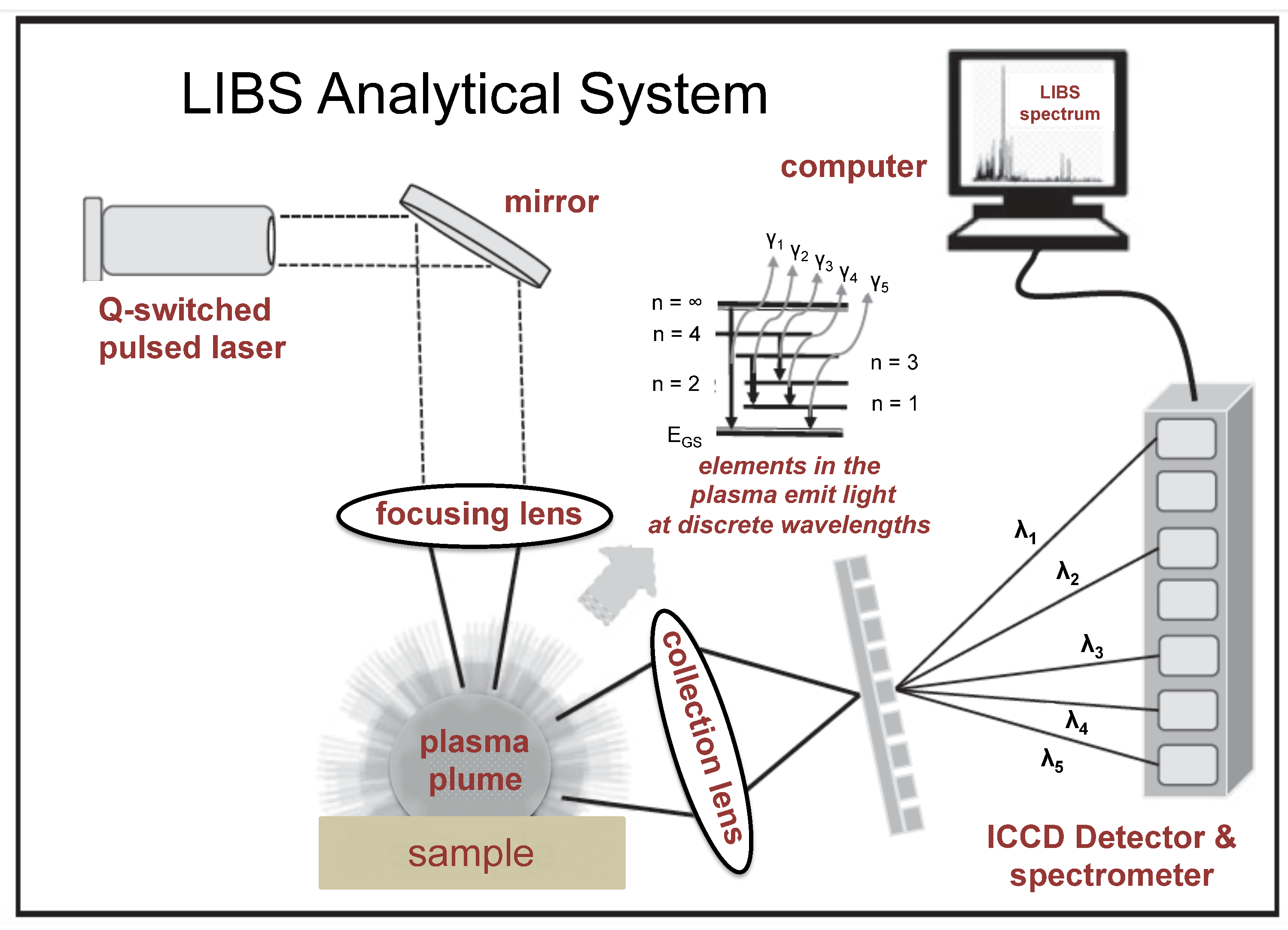
2. Laser-Induced Breakdown Spectroscopy
2.1. The LIBS Analysis
2.2. Specific Attributes of LIBS
2.3. LIBS for Ore Prospecting
3. Analytical Methods
4. Results and Discussion
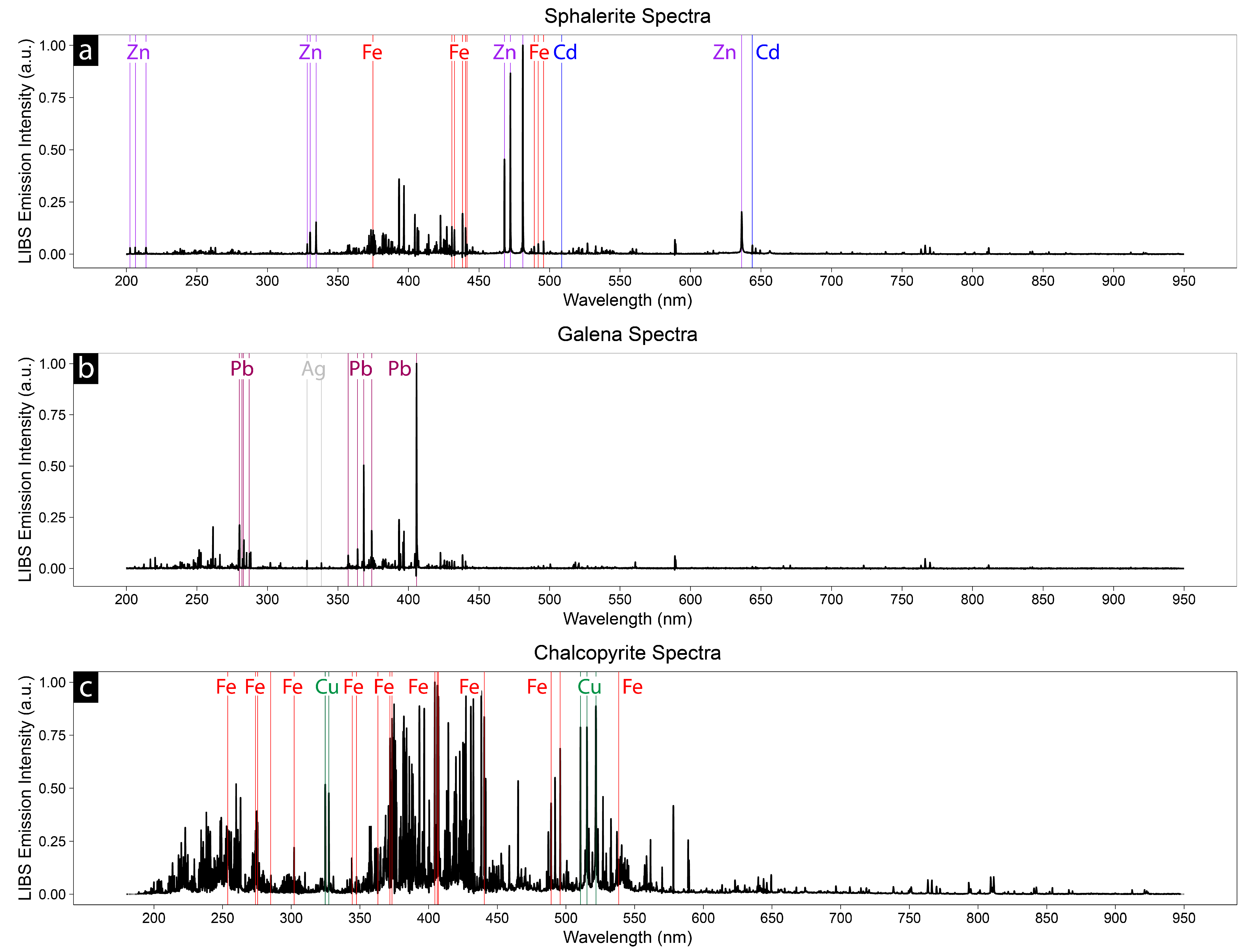
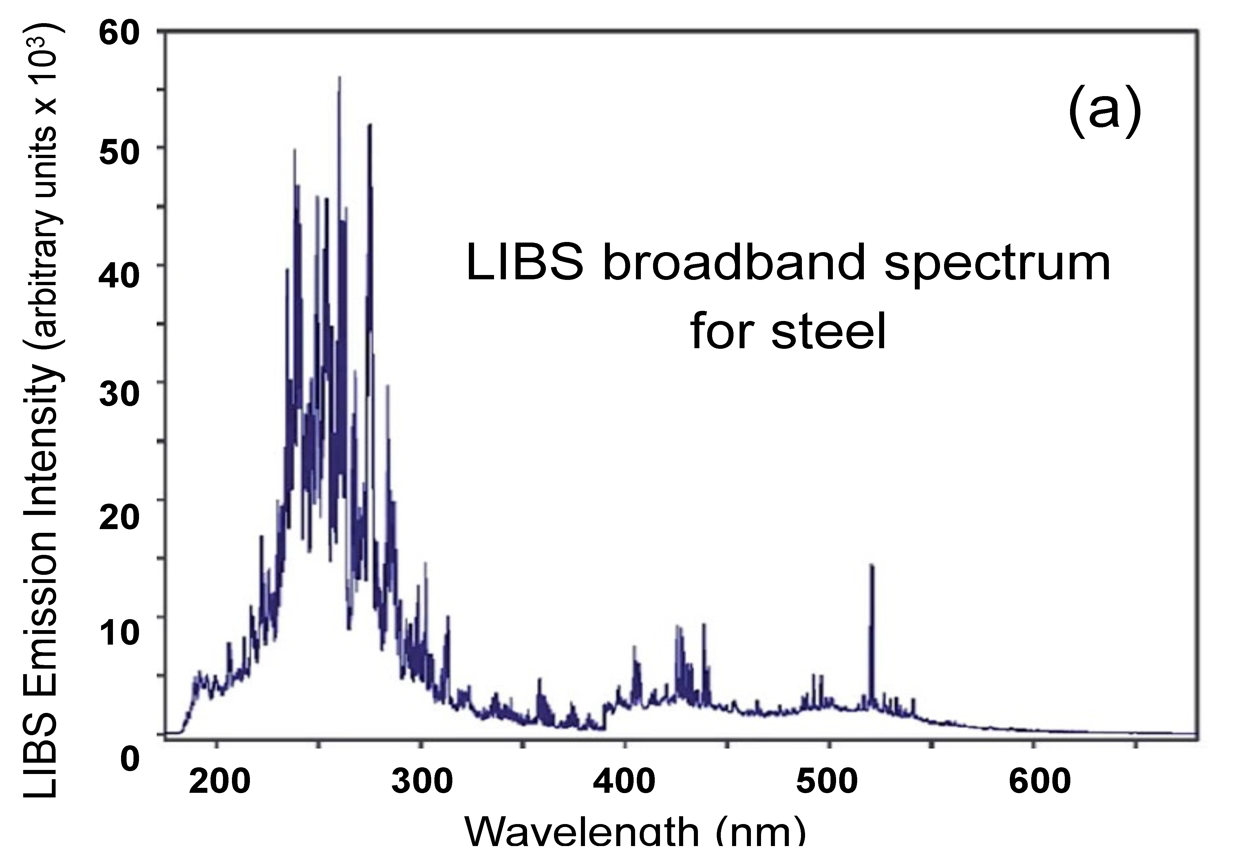
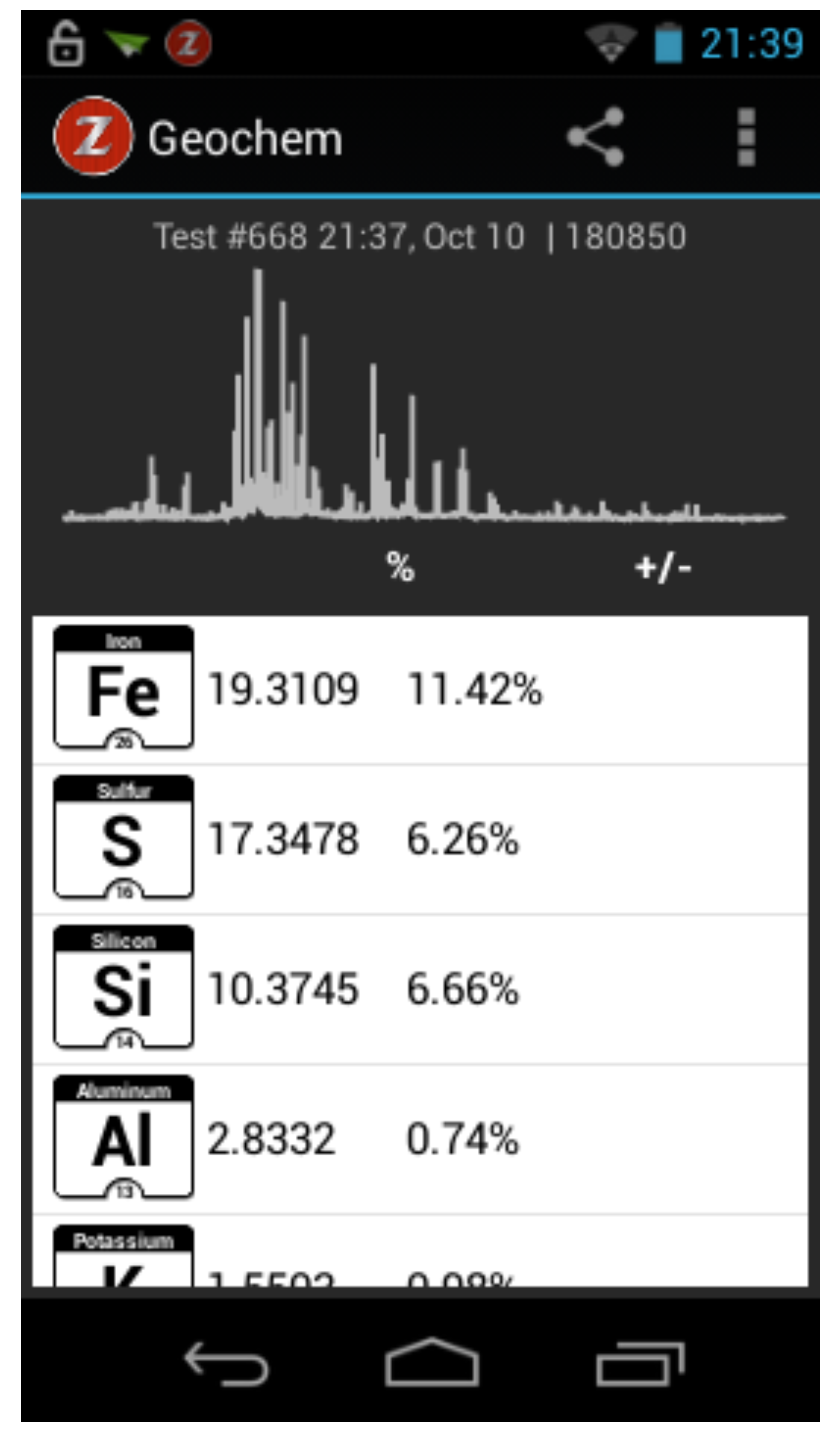
4.1. Elemental Detection and Qualitative Analysis
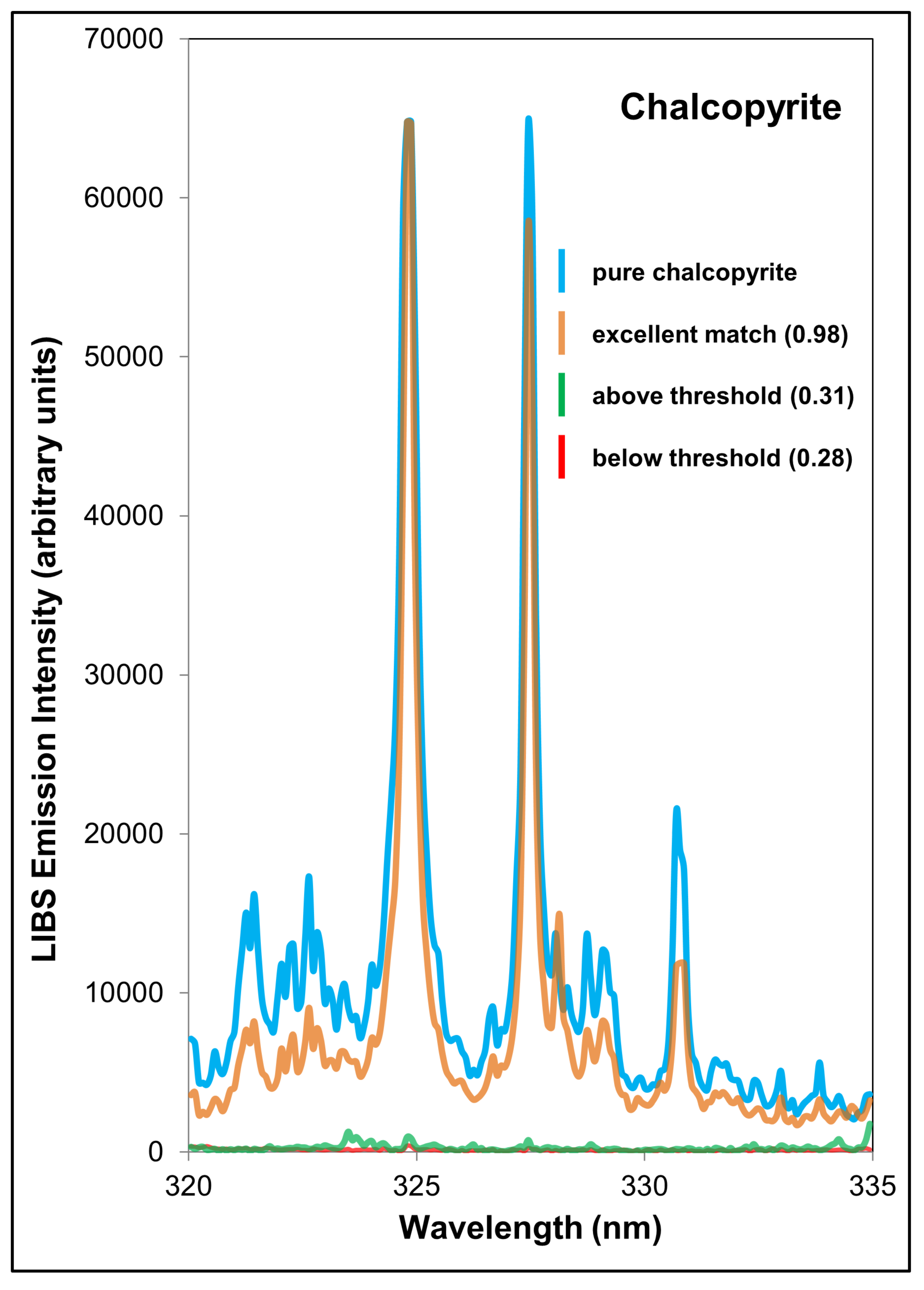
4.1.1. Chemometrics
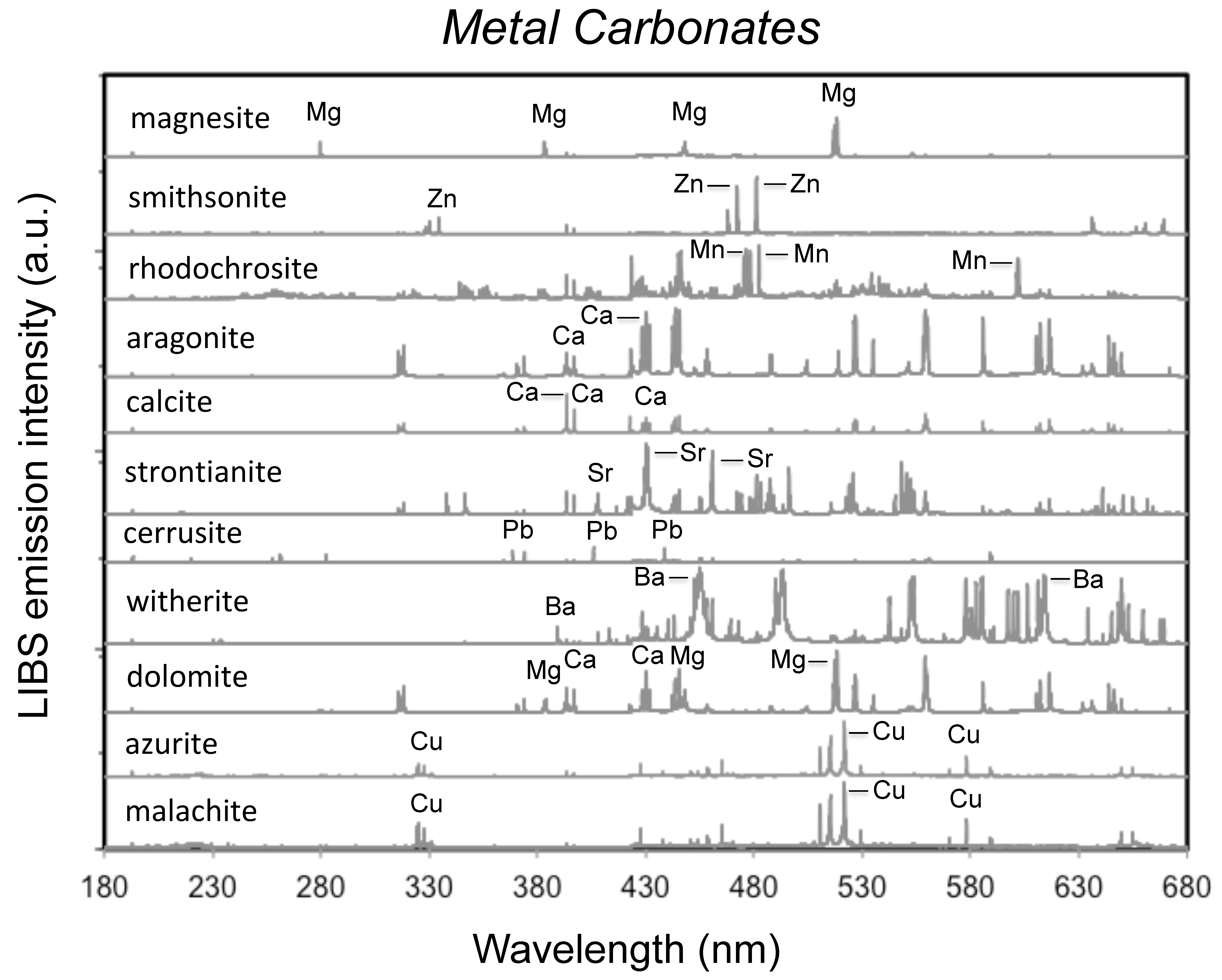
4.1.2. Metal Carbonates
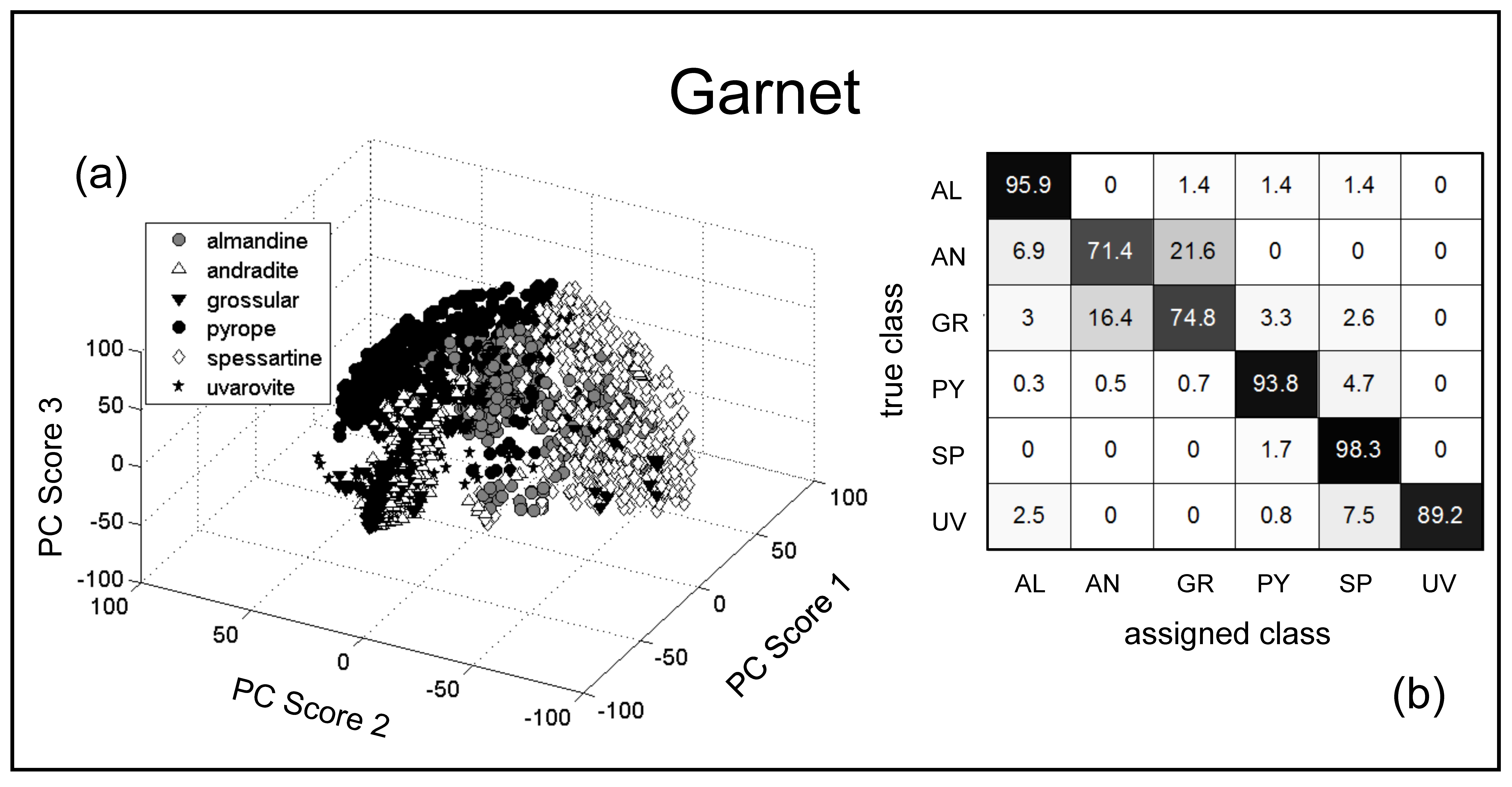
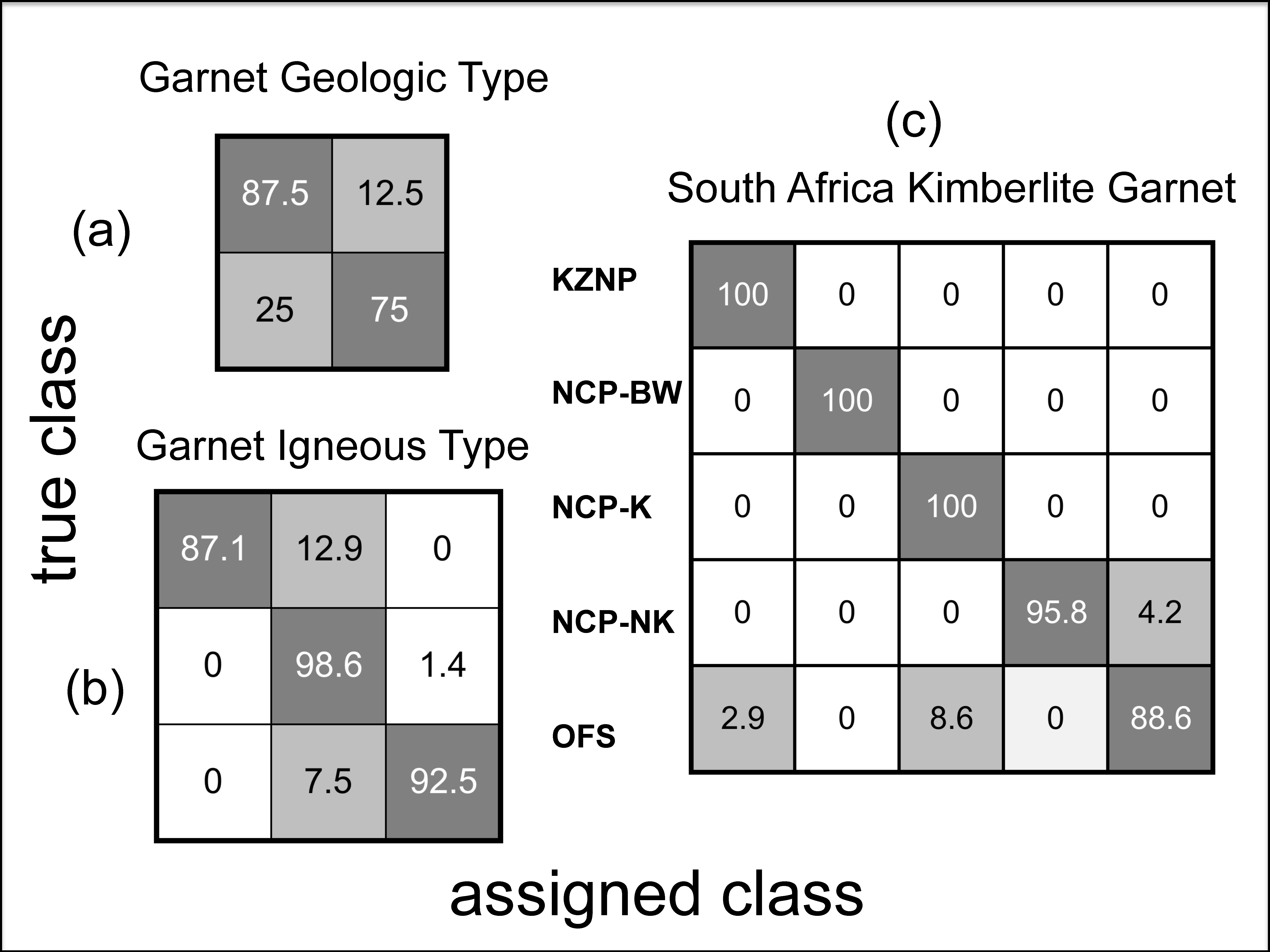
4.1.3. Garnet
4.1.4. Oxide Minerals
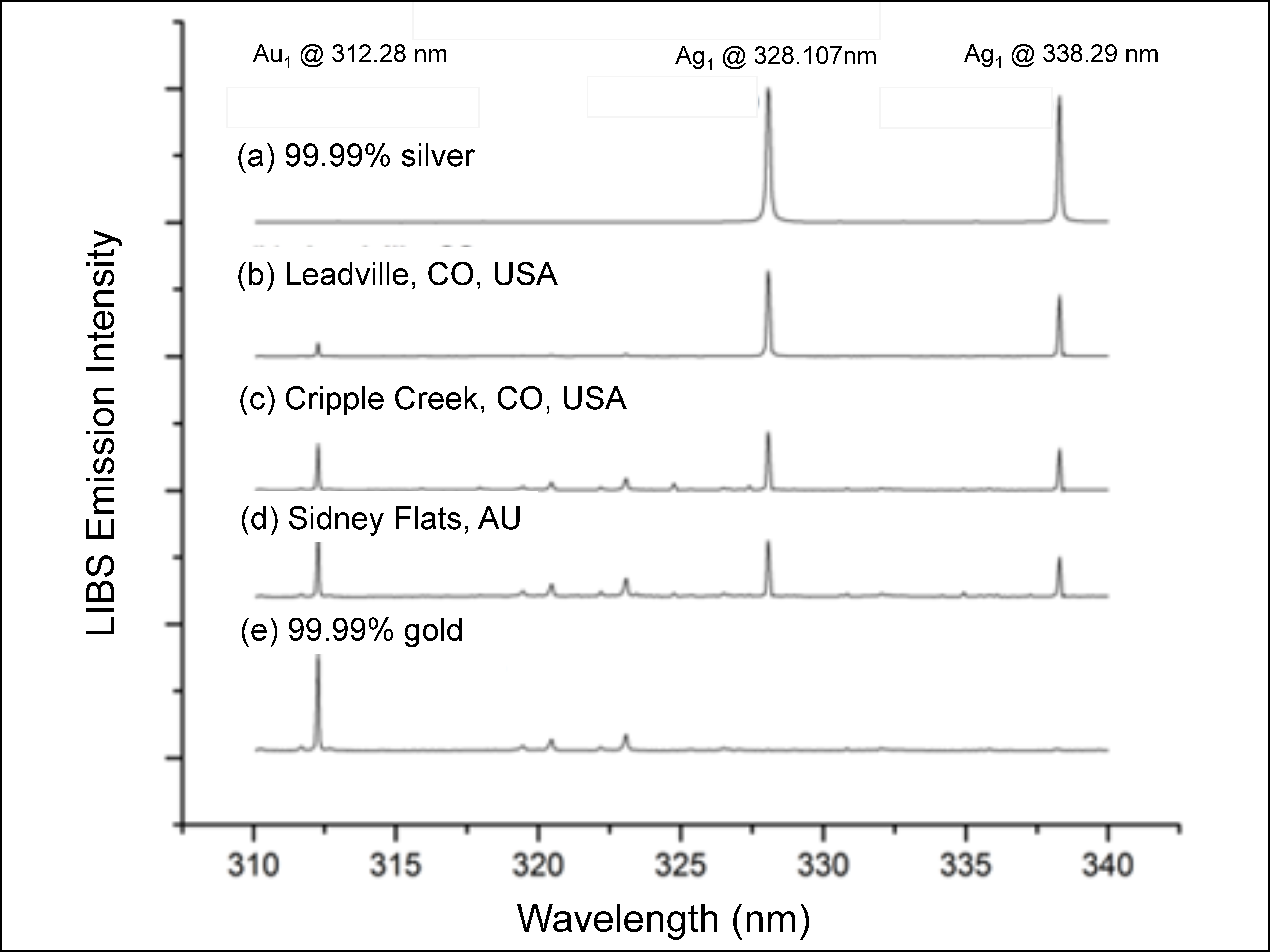
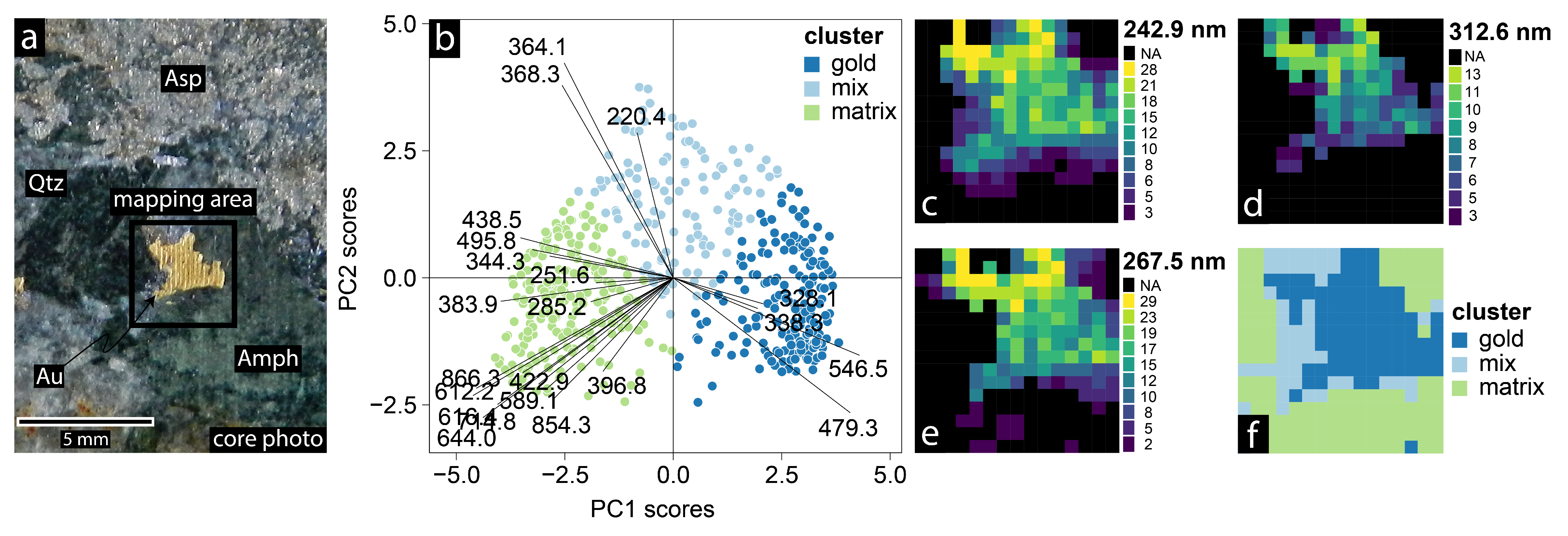
4.1.5. Gold
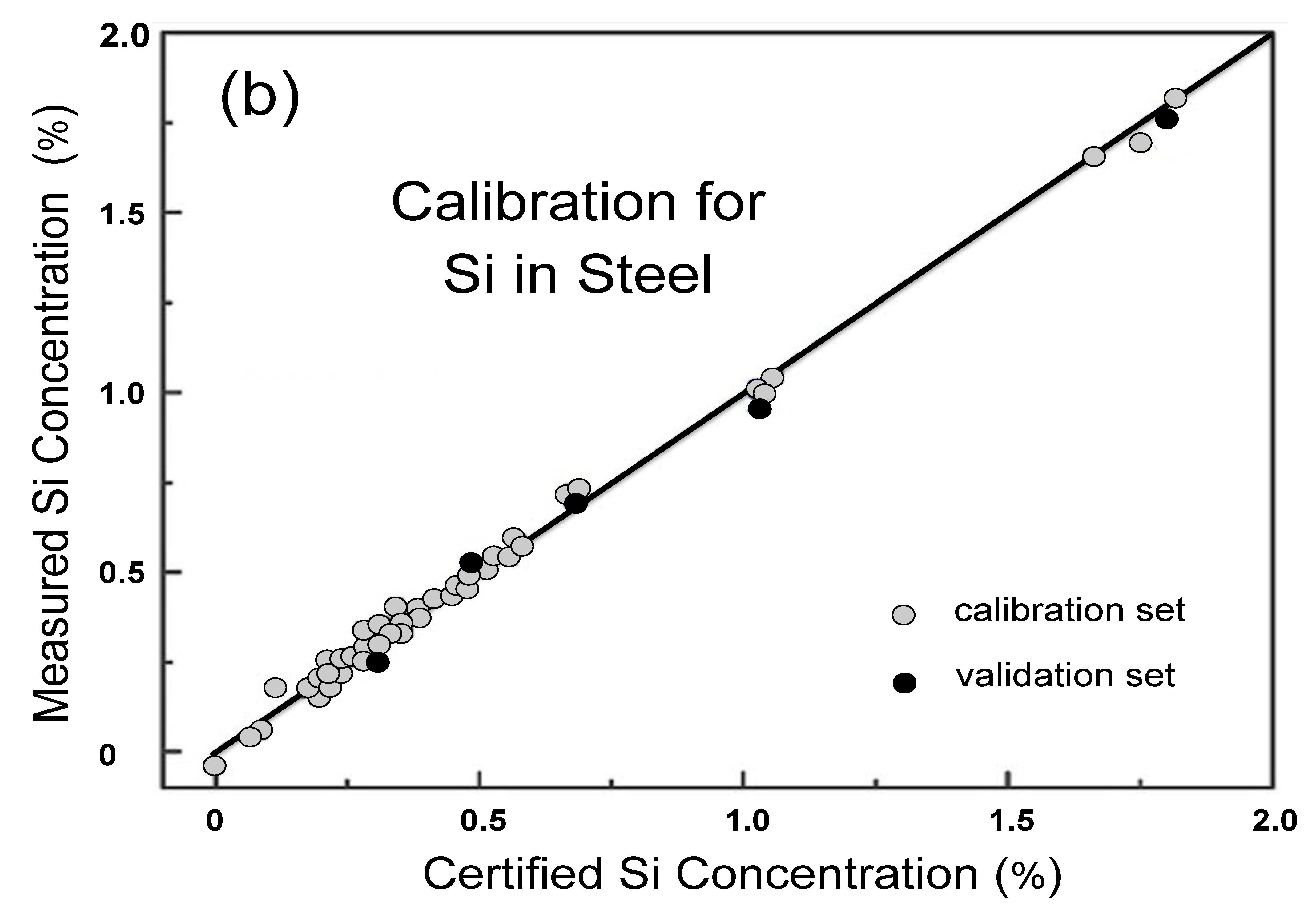
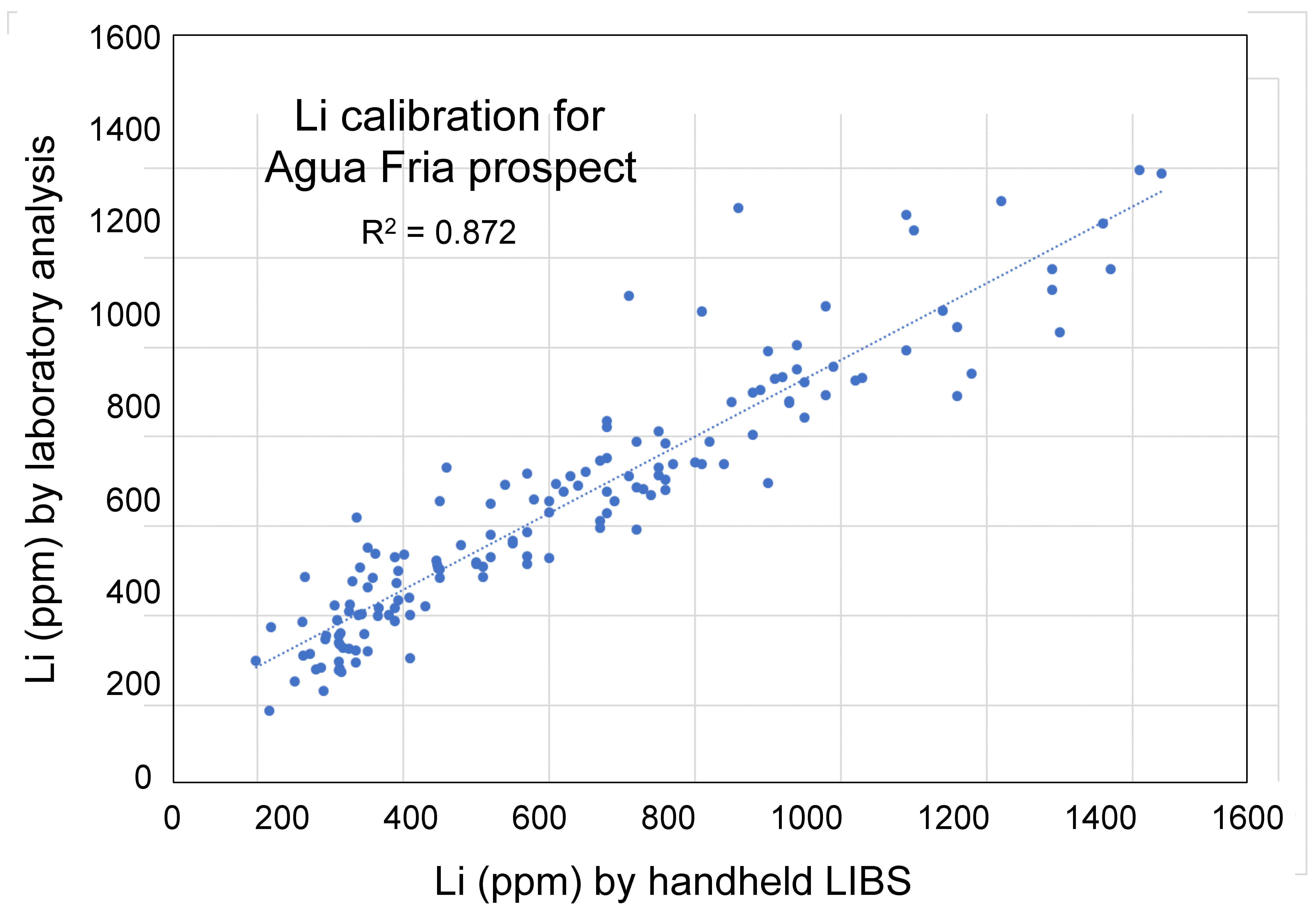
4.2. Quantitative Analysis
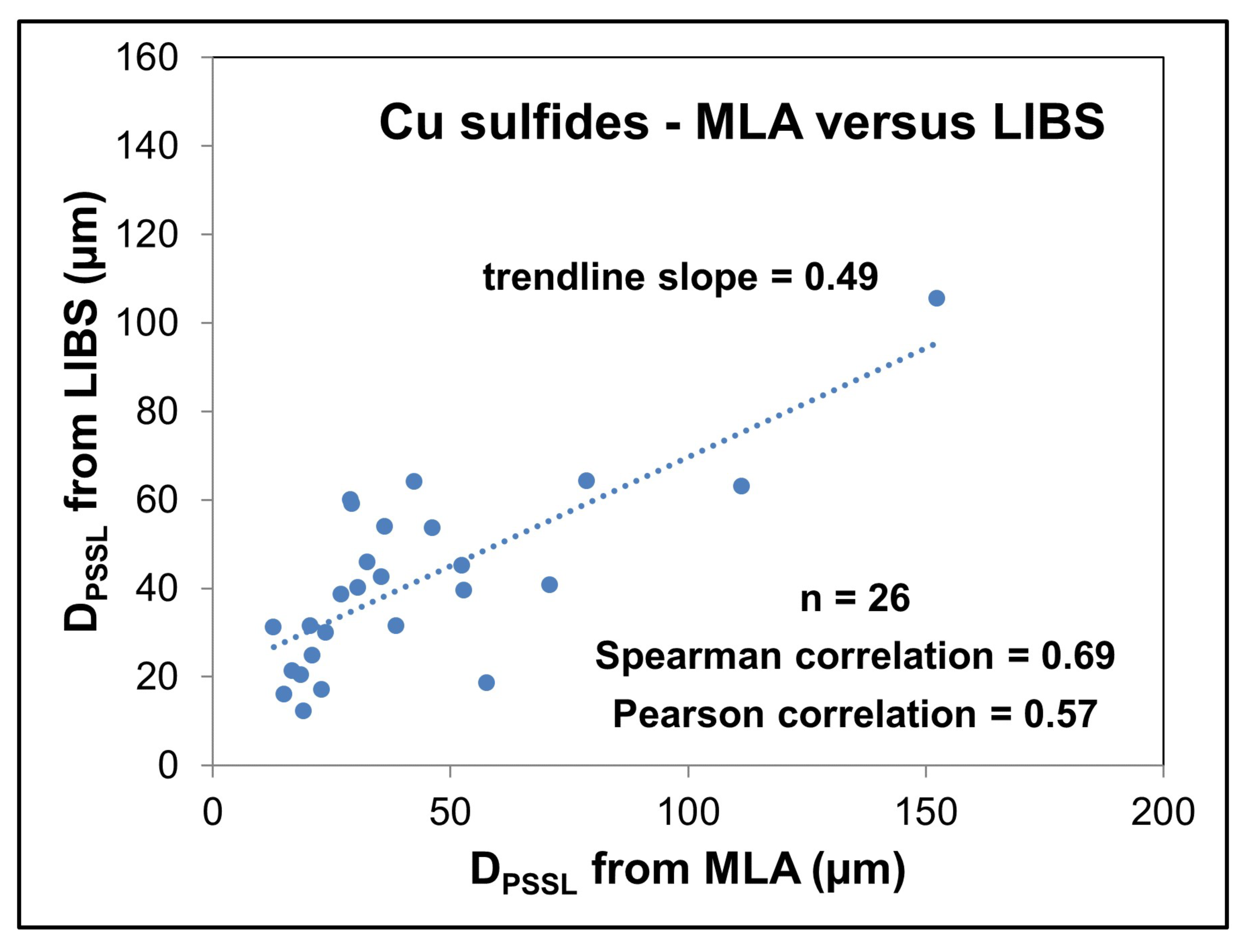
4.3. Grain Size Analysis
4.3.1. Introduction
4.3.2. Methodology
Data Collection
Selection of Spectral Lines and Background
Grain Size Proxy Calculations
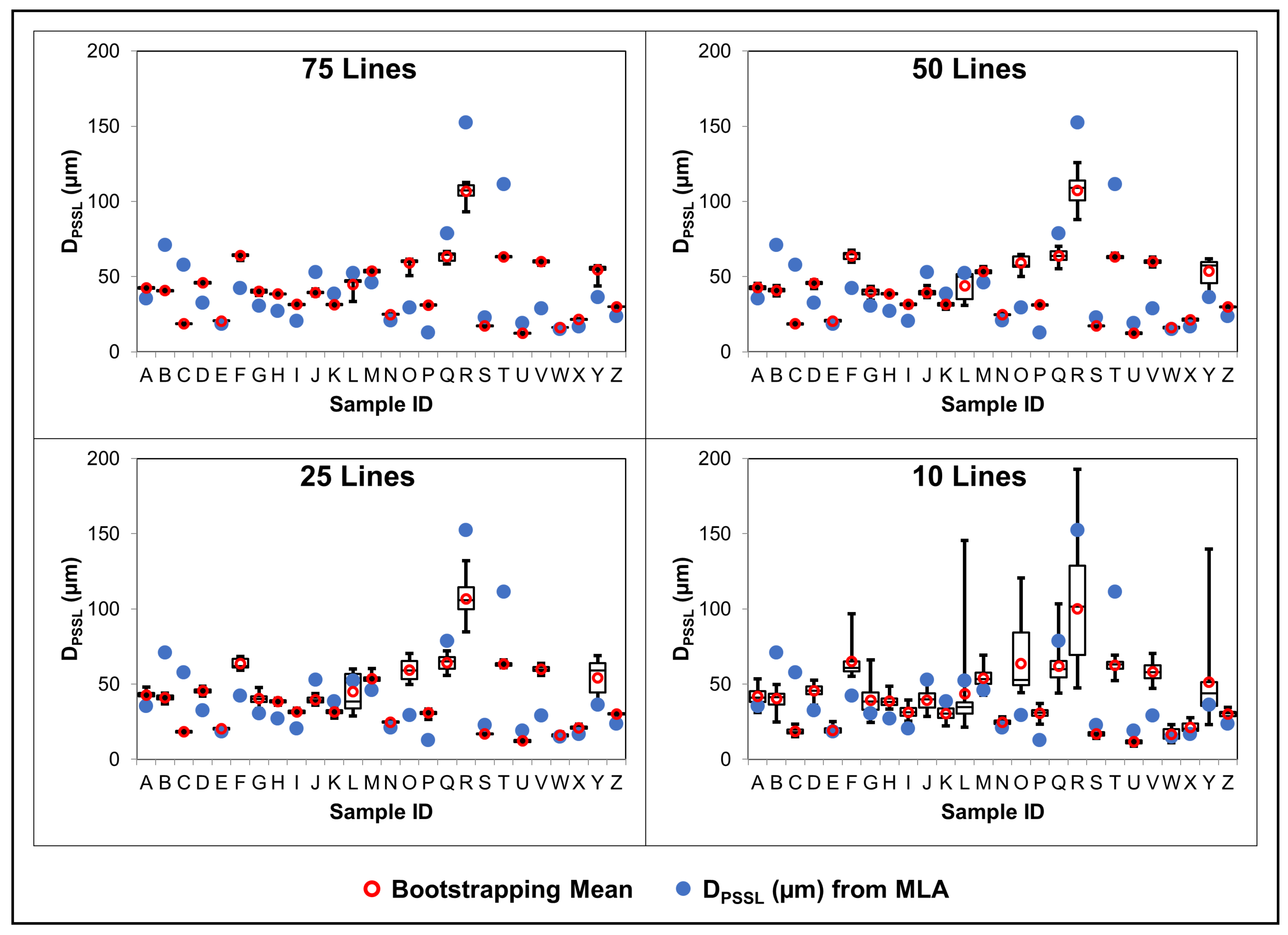
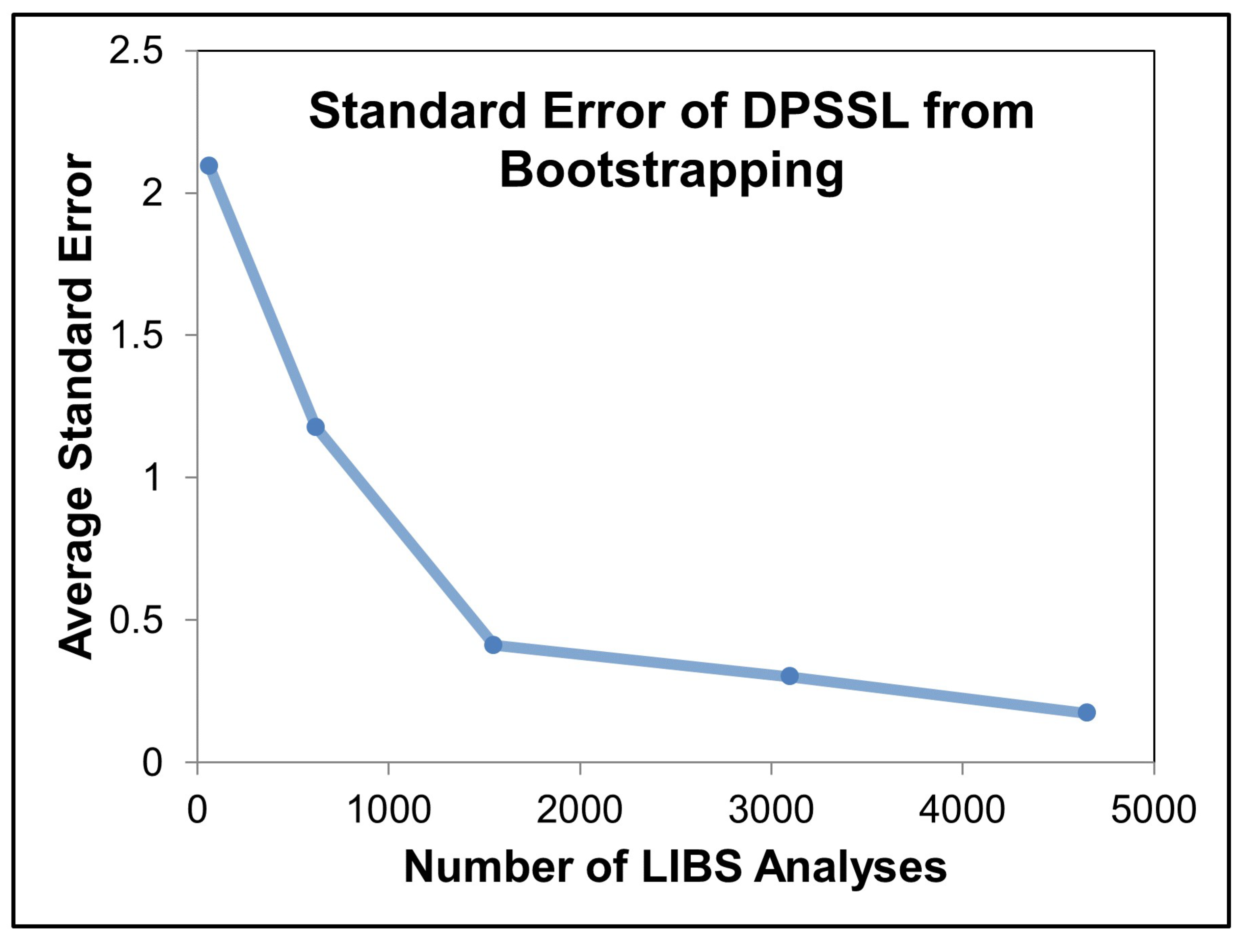
4.3.3. Results
4.3.4. Discussion
4.3.5. Conclusions
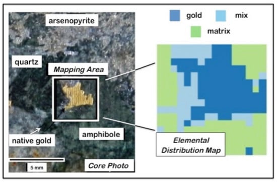
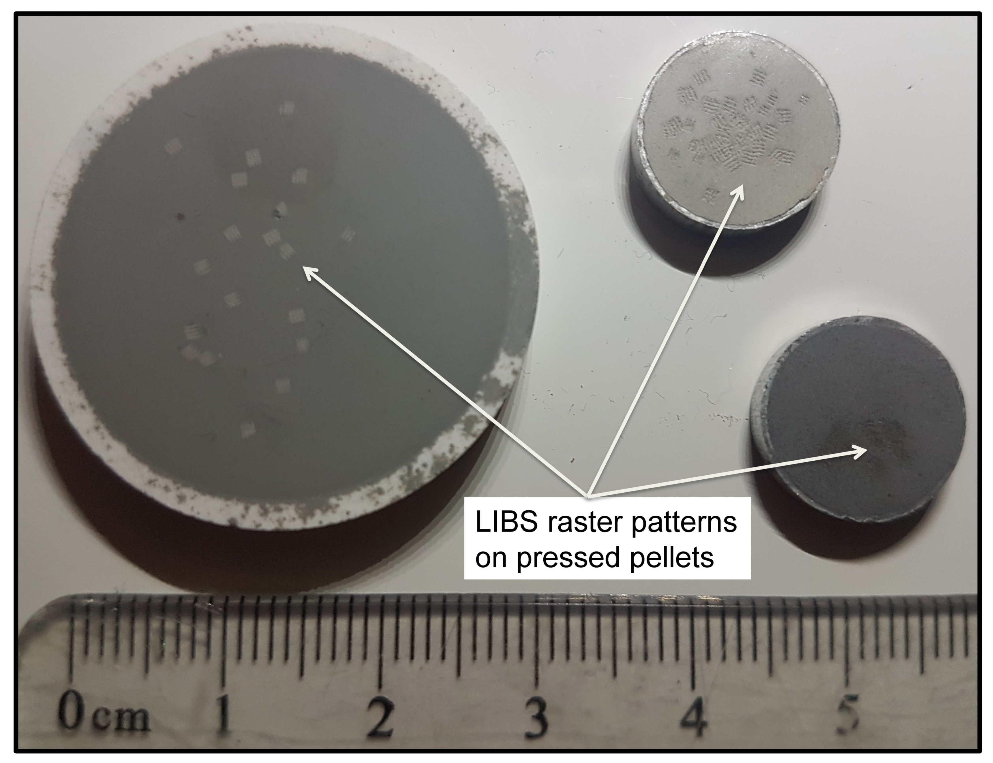
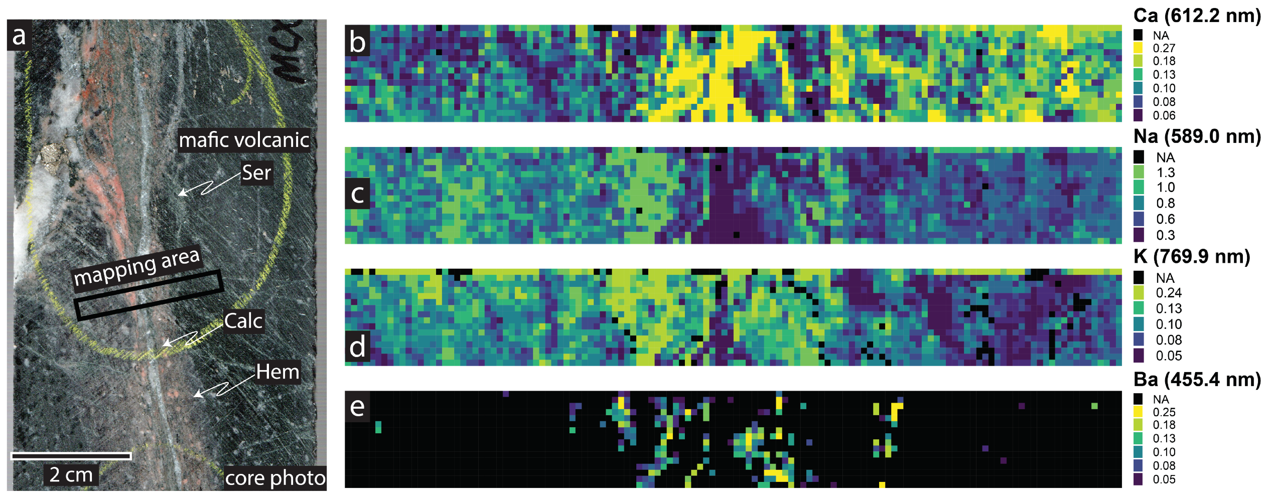
4.4. Geochemical Imaging and Microscale Mapping
4.4.1. Introduction
4.4.2. Methodology
4.4.3. Results
5. Summary and Future Prospects
Author Contributions
Funding
Acknowledgments
Conflicts of Interest
References
- Meinert, L.D.; Robinson, G.; Nassar, N.T. Mineral resources: Reserves, peak production and the future. Resources 2016, 5, 14. [Google Scholar] [CrossRef]
- Lusty, P.; Gunn, A. Challenges to global mineral resource security and options for future supply. In Ore Deposits in An Evolving Earth; Special Publications; Jenkin, G., Lusty, P., McDonald, I., Smith, M., Boyce, A., Wilkinson, J., Eds.; Geological Society: London, UK, 2019; Volume 393, pp. 265–276. [Google Scholar]
- Ali, S.; Giurco, D.; Arndt, N.; Nickless, E.; Brown, G.; Demetriades, A.; Durrheim, R.; Enriquez, M.; Kinnaird, J.; Littleboy, A.; et al. Mineral supply for sustainable development requires resource governance. Nature 2017, 543, 367–372. [Google Scholar] [CrossRef] [PubMed]
- Arndt, N.; Fontboté, L.; Hedenquist, J.; Kesler, S.; Thompson, J.; Wood, D. Future global mineral resources. Geochem. Perspect. 2017, 6, 171. [Google Scholar] [CrossRef]
- Skirrow, R.; Huston, D.; Mernagh, T.; Thorne, J.; Dulfer, H.; Senior, A. Critical Commodities for A High-Tech World: Australia′s Potential to Supply Global Demand; Geoscience Australia: Canberra, Australia, 2013; p. 126. [Google Scholar]
- Mudd, G.M.; Jowitt, S.M.; Werner, T.T. The world′s by-product and critical metal resources part I: Uncertainties, current reporting practices, implications and grounds for optimism. Ore Geol. Rev. 2017, 86, 924–938. [Google Scholar] [CrossRef]
- Sillitoe, R. Grassroots Exploration: Between a Major Rock and a Junior Hard Place. Soc. Econ. Geol. Newsl. 2010, 83, 11–13. [Google Scholar]
- Beaty, R. The Declining Discovery Trend: People, Science or Scarcity? Soc. Econ. Geol. Newsl. 2010, 81, 14–18. [Google Scholar]
- Duke, J. Government Geoscience to Support Mineral Exploration: Public Policy Rationale and Impact; Prospectors and Developers Association of Canada, PDAC: Toronto, ON, Canada, 2010; p. 72. [Google Scholar]
- Blain, C. Fifty-year trends in minerals discovery—Commodity and ore-type targets. Explor. Min. Geol. 2001, 9, 1–11. [Google Scholar] [CrossRef]
- Wood, D. Mineral Resource Discovery—Science, Art & Business. Soc. Econ. Geol. Newsl. 2010, 80, 12–17. [Google Scholar]
- Hagemann, S.G.; Lisitsin, V.A.; Huston, D.L. Mineral system analysis: Quo vadis. Ore Geol. Rev. 2016, 76, 504–522. [Google Scholar] [CrossRef]
- McCuaig, T.C.; Beresford, S.; Hronsky, J. Translating the mineral systems approach into an effective exploration targeting system. Ore Geol. Rev. 2010, 38, 128–138. [Google Scholar] [CrossRef]
- Huston, D.L.; Mernagh, T.P.; Hagemann, S.G.; Doublier, M.P.; Fiorentini, M.; Champion, D.C.; Jaques, A.L.; Czarnota, K.; Cayley, R.; Skirrow, R.; et al. Tectono-metallogenic systems—The place of mineral systems within tectonic evolution, with an emphasis on Australian examples. Ore Geol. Rev. 2016, 76, 168–210. [Google Scholar] [CrossRef]
- Rogers, N. Targeted Geoscience Initiative: 2018 report of activities. Geol. Surv. Can. Open File 8549 2018, 2, 448. [Google Scholar]
- Wyborn, L.; Heinrich, C.; Jaques, A. Australian Proterozoic mineral systems: Essential ingredients and mappable criteria. In The AusIMM Annual Conference Proceedings; AusIMM Darwin: Northern Territory, Australia, 1994; pp. 109–115. [Google Scholar]
- Gaillard, N.; Williams-Jones, A.E.; Clark, J.R.; Lypaczewski, P.; Salvi, S.; Perrouty, S.; Piette-Lauzière, N.; Guilmette, C.; Linnen, R.L. Mica composition as a vector to gold mineralization: Deciphering hydrothermal and metamorphic effects in the Malartic district, Quebec. Ore Geol. Rev. 2018, 95, 789–820. [Google Scholar] [CrossRef]
- Noble, R.; Christie, A. Update on exploration geochemistry initiatives in Australia and New Zealand. Explore 2015, 166, 13–17. [Google Scholar]
- Lesher, C.; Hannington, M.; Galley, A. Integrated multi-parameter exploration footprints of the Canadian Malartic disseminated Au, McArthur River-Millennium unconformity U, and Highland Valley porphyry Cu Deposits: Preliminary results from the NSERC-CMIC Mineral Exploration Footprints Research. Proc. Explor. 2017, 17, 23. [Google Scholar]
- De Caritat, P.; Main, P.T.; Grunsky, E.C.; Mann, A.W. Recognition of geochemical footprints of mineral systems in the regolith at regional to continental scales. Aust. J. Earth Sci. 2017, 64, 1033–1043. [Google Scholar] [CrossRef]
- Vallée, M.A.; Morris, W.A.; Perrouty, S.; Lee, R.G.; Wasyliuk, K.; King, J.J.; Ansdell, K.; Mir, R.; Shamsipour, P.; Farquharson, C.G.; et al. Geophysical inversion contributions to mineral exploration: Lessons from the Footprints project. Can. J. Earth Sci. 2019, 543, 525–543. [Google Scholar] [CrossRef]
- Halley, S.; Dilles, J.; Tosdal, R. Footprints: Hydrothermal alteration and geochemical dispersion around porphyry copper deposits. Soc. Econ. Geol. Newsl. 2015, 100, 12–17. [Google Scholar]
- Winterburn, P.A.; Noble, R.R.P.; Lawie, D. Advances in exploration geochemistry, 2007 to 2017 and beyond. Geochem. Explor. Environ. Anal. 2019, 30, 10. [Google Scholar] [CrossRef]
- Kyser, K.; Barr, J.; Ihlenfeld, C. Applied geochemistry in mineral exploration and mining. Elements 2015, 11, 241–246. [Google Scholar] [CrossRef]
- Noll, R. Laser-Induced Breakdown Spectroscopy: Fundamentals and Applications; Springer: Berlin, Germany, 2012. [Google Scholar]
- Cremers, D.; Radziemski, L. Handbook of Laser-Induced Breakdown Spectroscopy; Wiley: Hoboken, NJ, USA, 2013. [Google Scholar]
- Lee, Y.; Song, K.; Sneddon, J. Laser-induced Breakdown Spectrometry; Nova Publishers: Hauppauge, NY, USA, 2000. [Google Scholar]
- Miziolek, A.; Palleschi, V.; Schechter, I. (Eds.) Laser Induced Breakdown Spectroscopy; Cambridge University Press: Cambridge, UK, 2006. [Google Scholar]
- Singh, J.; Thakur, S. (Eds.) Laser-Induced Breakdown Spectroscopy; Elsevier: Amsterdam, The Netherlands, 2007. [Google Scholar]
- Musazzi, S.; Perini, U. (Eds.) Laser-Induced Breakdown Spectroscopy, Theory and Applications; Springer: Berlin, Germany, 2014. [Google Scholar]
- Rusak, D.; Castle, B.; Smith, B.; Winefordner, J. Fundamentals and applications of laser-induced breakdown spectroscopy. Crit. Rev. Anal. Chem. 1997, 27, 257–290. [Google Scholar] [CrossRef]
- Harmon, R.; Russo, R.; Hark, R. Applications of laser-induced breakdown spectroscopy for geochemical and environmental analysis: A comprehensive review. Spectrochim. Acta Part B 2013, 87, 11–26. [Google Scholar] [CrossRef]
- Fabre, C.; Boiron, M.; Dubessy, I.; Cathelineau, M.; Banks, D. Palaeofluid chemistry of a single fluid event: A bulk and in-situ multi-technique analysis (LIBS, Raman Spectroscopy) of an Alpine fluid (Mont-Blanc). Chem. Geol. 2002, 182, 249. [Google Scholar] [CrossRef]
- Stipe, C.; Miller, A.; Brown, J.; Guevara, E.; Cauda, E. Evaluation of laser-induced breakdown spectroscopy (LIBS) for measurement of silica on filter samples of coal dust. Appl. Spectrosc. 2012, 66, 1286–1293. [Google Scholar] [CrossRef]
- Tognoni, E.; Cristoforetti, G.; Legnaiolia, S.; Palleschi, V. Calibration-free laser-induced breakdown spectroscopy: State of the art. Spectrochim. Acta Part B 2010, 65, 1–14. [Google Scholar] [CrossRef]
- Praher, B.; Palleschi, V.; Viskup, P.; Heitz, J.; Pedarnig, J. Calibration free laser induced breakdown spectroscopy of oxide materials. Spectrochim. Acta Part B 2010, 65, 671–679. [Google Scholar] [CrossRef]
- Winefordner, J.; Gornushkin, I.; Correll, T.; Gibb, E.; Smith, B.; Omenetto, N. Comparing several atomic spectrometric methods to the super stars: Special emphasis on laser induced breakdown spectrometry, LIBS, a future super star. J. Anal. At. Spectrom. 2004, 19, 1061–1083. [Google Scholar] [CrossRef]
- Hahn, D.; Flower, W.; Hencken, K. Discrete particle detection and metal emissions monitoring using laser-induced breakdown spectroscopy. Appl. Spectrosc. 1997, 51, 1836–1844. [Google Scholar] [CrossRef]
- Derome, D.; Cathelineau, M.; Cuney, M.; Fabre, C.; Lhomme, T.; Banks, D. Mixing of sodic and calcic brines and uranium deposition at McArthur River, Saskatchewan, Canada: A Raman and laser-induced breakdown spectroscopic study of fluid inclusions. Econ. Geol. 2005, 100, 1529–1545. [Google Scholar] [CrossRef]
- Lebedev, V.; Makarchuk, P.; Stepanov, D. Real-time qualitative study of forsterite crystal–Melt lithium distribution by laser-induced breakdown spectroscopy. Spectrochim. Acta Part B 2017, 137, 23–27. [Google Scholar] [CrossRef]
- Fabre, C.; Devismes, D.; Moncayo, S.; Pelascini, F.; Trichard, F.; Leocmte, A.; Bousquet, B.; Cauzid, J.; Motto-Ros, V. Elemental imaging by laser-induced breakdown spectroscopy for the geological characterization of minerals. J. Anal. At. Spectrom. 2018, 33, 1345–1353. [Google Scholar] [CrossRef]
- Kim, T.; Lin, C.; Yoon, Y. Compositional mapping by laser-induced breakdown spectroscopy. J. Phys. Chem. B 1998, 102, 4284–4287. [Google Scholar] [CrossRef]
- Cabalín, L.; Mateo, M.; Laserna, J. Chemical maps of patterned samples by microline-imaging laser-induced plasma spectrometry. Surf. Interface Anal. 2003, 35, 263–267. [Google Scholar] [CrossRef]
- Novotný, K.; Kaiser, J.; Galiová, M.; Konečna, V.; Novotný, J.; Malina, R.; Liška, M.; Kanický, V. Mapping of different structures on large area of granite sample using laser-ablation based analytical techniques, an exploratory study. Spectrochim. Acta Part B 2008, 63, 1139–1144. [Google Scholar] [CrossRef]
- Sweetapple, M.; Tassios, S. Laser-induced breakdown spectroscopy (LIBS) as a tool for in situ mapping and textural interpretation of lithium in pegmatite minerals. Am. Mineral. 2015, 100, 2141–2151. [Google Scholar] [CrossRef]
- Kuhn, K.; Meima, J.; Rammlmair, D.; Ohlendorf, C. Chemical mapping of mine waste drill cores with laser-induced breakdown spectroscopy (LIBS) and energy dispersive X-ray fluorescence (EDXRF) for mineral resource exploration. J. Geochem. Explor. 2016, 161, 72–84. [Google Scholar] [CrossRef]
- Rifai, K.; Laflamme, M.; Constantin, M.; Vidal, F.; Sabsabi, M.; Blouin, A.; Bouchard, P.; Fytas, K.; Castello, M.; Kamwa, N. Analysis of gold in rock samples using laser-induced breakdown spectroscopy: Matrix and heterogeneity effects. Spectrochim. Acta Part B 2017, 134, 33–41. [Google Scholar] [CrossRef]
- Maravlekai, P.; Zafiropulos, V.; Kilikoglou, V.; Kalaitzaki, M.; Fotakis, C. Laser-induced breakdown spectroscopy as a diagnostic technique for the laser cleaning of marble. Spectrochim. Acta Part B 1997, 52, 41–53. [Google Scholar] [CrossRef]
- Ortiz, P.; Vázquez, M.; Ortiz, R.; Martin, J.; Ctvrnickova, T.; Mateo, M.; Nicolas, G. Investigation of environmental pollution effects on stone monuments in the case of Santa Maria La Blanca, Seville (Spain). Appl. Phys. A 2010, 100, 965–973. [Google Scholar] [CrossRef]
- Kaski, S.; Häkkänen, H.; Korppi-Tommola, J. Sulfide mineral identification using laser-induced plasma spectroscopy. Miner. Eng. 2003, 16, 1239–1243. [Google Scholar] [CrossRef]
- Haavisto, O.; Kauppinen, T.; Häkkänen, H. Laser-induced breakdown spectroscopy for rapid elemental analysis of drillcore. IFAC Proc. Vol. 2013, 46, 87–91. [Google Scholar] [CrossRef]
- Popov, A.; Labutin, T.; Zaytsev, S.; Seliverstova, I.; Zorov, N.; Kal′ko, I.; Sidorina, Y.; Bugaev, I.; Nikolaev, Y. Determination of Ag, Cu, Mo and Pb in soils and ores by laser-induced breakdown spectrometry. J. Anal. At. Spectrom. 2014, 29, 1925–1933. [Google Scholar] [CrossRef]
- Díaz, D.; Hahn, D.; Molina, A. Quantification of gold and silver in minerals by laser-induced breakdown spectroscopy. Spectrochim. Acta Part B 2017, 136, 106–115. [Google Scholar] [CrossRef]
- Rifai, K.; Doucet, F.; Özcan, L.; Vidal, F. LIBS core imaging at kHz speed: Paving the way for real-time geochemical applications. Spectrochim. Acta Part B 2018, 150, 43–48. [Google Scholar] [CrossRef]
- Zorba, V.; Mao, X.; Russo, R. Ultrafast laser induced breakdown spectroscopy for high spatial resolution chemical analysis. Spectrochim. Acta Part B 2011, 66, 189–192. [Google Scholar] [CrossRef]
- Čtvrtníčková, T.; Fortes, F.; Cabalin, L.; Laserna, J. Optical restriction of plasma emission light for nanometric sampling depth and depth profiling of multilayered metal samples. Appl. Spectrosc. 2007, 61, 719–724. [Google Scholar] [CrossRef] [PubMed]
- Čtvrtníčková, T.; Fortes, F.; Cabalin, L.; Kanický, V.; Laserna, J. Depth profiles of ceramic tiles by using orthogonal double-pulse laser induced breakdown spectrometry. Surf. Interface Anal. 2009, 41, 714–719. [Google Scholar] [CrossRef]
- Yamamoto, K.; Cremers, D.; Ferris, M.; Foster, L. Detection of metals in the environment using a portable laser-induced breakdown spectroscopy instrument. Appl. Spectrosc. 1996, 50, 222–233. [Google Scholar] [CrossRef]
- Wainner, R.; Harmon, R.; Miziolek, A.; McNesby, K.; French, P. Analysis of environmental lead contamination: Comparison of LIBS field and laboratory instruments. Spectrochim. Acta Part B 2001, 56, 777–793. [Google Scholar] [CrossRef]
- Palanco, S.; Alises, A.; Cunat, J.; Baena, J.; Laserna, J. Development of a portable laser-induced plasma spectrometer with fully-automated operation and quantitative analysis capabilities. J. Anal. At. Spectrom. 2003, 18, 933–938. [Google Scholar] [CrossRef]
- Goujon, J.; Giakoumaki, A.; Piñon, V.; Musset, O.; Georgiou, E.; Boquillon, J. A compact and portable laser-induced breakdown spectroscopy instrument for single and double pulse applications. Spectrochim. Acta Part B 2008, 63, 1091–1096. [Google Scholar] [CrossRef]
- Cuñat, J.; Fortes, F.; Cabalín, L.; Carrasco, F.; Simón, M.; Laserna, J. Man-portable laser-induced breakdown spectroscopy system for in situ characterization of karstic formations. Appl. Spectrosc. 2008, 62, 1250–1255. [Google Scholar] [CrossRef]
- Rakovský, J.; Musset, O.; Buoncristiani, J.; Bichet, V.; Monna, F.; Neige, P.; Veis, P. Testing a portable laser-induced breakdown spectroscopy system on geological samples. Spectrochim. Acta Part B 2012, 74, 57–65. [Google Scholar] [CrossRef]
- Bertolini, A.; Carelli, G.; Francesconi, F.; Francesconi, M.; Marchesini, L.; Marsili, P.; Sorrentino, F.; Cristoforetti, G.; Legnaioli, S.; Palleschi, V.; et al. Modì: A new mobile instrument for in situ double-pulse LIBS analysis. Anal. Bioanal. Chem. 2006, 385, 240–247. [Google Scholar] [CrossRef]
- Connors, B.; Somers, A.; Day, D. Application of handheld laser-induced breakdown spectroscopy (LIBS) to geochemical analysis. Appl. Spectrosc. 2016, 70, 810–815. [Google Scholar] [CrossRef] [PubMed]
- Radziemski, L. From LASER to LIBS, the path of technology development. Spectrochim. Acta Part B 2002, 57, 1109–1113. [Google Scholar] [CrossRef]
- Bogue, R. Boom time for LIBS technology. Sens. Rev. 2004, 24, 353–357. [Google Scholar] [CrossRef]
- McMillan, N.; McManus, C.; Harmon, R.; DeLucia, F.; Miziolek, A. Laser-induced breakdown spectroscopy analysis of complex silicate minerals—Beryl. Anal. Bioanal. Chem. 2006, 385, 263–271. [Google Scholar] [CrossRef] [PubMed]
- Harmon, R.; Remus, J.; McMillan, N.; McManus, C.; Collins, L.; JL, G.; DeLucia, F.; Miziolek, A. LIBS analysis of geomaterials: Geochemical fingerprinting for the rapid analysis and discrimination of minerals. Appl. Geochem. 2009, 24, 1125–1141. [Google Scholar] [CrossRef]
- Grant, K.; Paul, G.; O′Neill, J. Time-resolved laser-induced breakdown spectroscopy of iron ore. Appl. Spectrosc. 1990, 44, 1711–1714. [Google Scholar] [CrossRef]
- Grant, K.; Paul, G.; O′Neill, J. Quantitative elemental analysis of iron ore by laser induced breakdown spectroscopy. Appl. Spectrosc. 1991, 45, 701–705. [Google Scholar] [CrossRef]
- Sun, Q.; Tran, M.; Smith, B.; Winefordner, J. Determination of Mn and Si in iron ore by laser induced plasma spectroscopy. Anal. Chim. Acta 2000, 413, 187–195. [Google Scholar] [CrossRef]
- Michaud, D.; Leclerc, R.; Proulx, É. Influence of particle size and mineral phase in the analysis of iron ore slurries by Laser-Induced Breakdown Spectroscopy. Spectrochim. Acta Part B 2007, 62, 1575–1581. [Google Scholar] [CrossRef]
- Death, D.; Cunningham, A.; Pollard, L. Multi-element analysis of iron ore pellets by laser induced breakdown spectroscopy and principal components regression. Spectrochim. Acta Part B 2008, 63, 763–769. [Google Scholar] [CrossRef]
- Gaft, M.; Sapir-Sofer, I.; Modiano, H.; Stana, R. Laser induced breakdown spectroscopy for bulk minerals online analyses. Spectrochim. Acta Part B 2007, 62, 1496–1503. [Google Scholar] [CrossRef]
- Rosenwasser, S.; Asimellis, G.; Bromley, B.; Hazlett, R.; Martin, J.; Pearce, T.; Zigler, A. Development of a method for automated quantitative analysis of ores using LIBS. Spectrochim. Acta Part B 2001, 56, 707–714. [Google Scholar] [CrossRef]
- Harhira, A.; Bouchard, P.; Rifai, K.; El Haddad, J.; Sabsabi, M.; Blouin, A.; Laflamme, M. Advanced Laser-induced breakdown spectroscopy (LIBS) sensor for gold mining. In Proceedings of the Conference of Metallurgists (COM), Vancouver, BC, Canada, 27–30 August 2017; p. 11. [Google Scholar]
- Díaz, D.; Molina, A.; Hahn, D. Effect of laser irradiance and wavelength on the analysis of gold-and silver-bearing minerals with laser-induced breakdown spectroscopy. Spectrochim. Acta Part B 2018, 145, 86–95. [Google Scholar] [CrossRef]
- Harmon, R.S.; Hark, R.R.; Throckmorton, C.S.; Rankey, E.C.; Wise, M.A.; Somers, A.M.; Collins, L.M. Geochemical fingerprinting by handheld laser-induced breakdown spectroscopy. Geostand. Geoanal. Res. 2017, 41, 563–584. [Google Scholar] [CrossRef] [Green Version]
- Somers, A. Application of hand-held laser induced breakdown spectroscopy to drilling samples: New technology providing new in-field analytical capabilities. In Proceedings of the Drilling for Geology II, Brisbane, Australia, 26–28 July 2017; pp. 89–96. [Google Scholar]
- Hoefs, J. Geochemical fingerprints: A critical appraisal. Eur. J. Mineral. 2010, 22, 3–15. [Google Scholar] [CrossRef] [Green Version]
- Gottfried, J.; Harmon, R.; De Lucia, F.; Miziolek, A. Multivariate analysis of laser-induced breakdown spectroscopy chemical signatures for geomaterial classification. Spectrochim. Acta Part B 2009, 64, 1009–1019. [Google Scholar] [CrossRef]
- Alvey, D.; Morton, K.; Harmon, R.; Gottfried, J.; Remus, J.; Collins, L.; Wise, M. Laser-induced breakdown spectroscopy-based geochemical fingerprinting for the rapid analysis and discrimination of minerals: The example of garnet. Appl. Opt. 2010, 49, C168–C180. [Google Scholar] [CrossRef] [Green Version]
- Hark, R.; Harmon, R. Geochemical fingerprinting using LIBS. In Laser-Induced Breakdown Spectroscopy–Theory & Applications; Musazzi, S., Perini, U., Eds.; Springer: Berlin, Germany, 2014; pp. 309–348. [Google Scholar]
- Harmon, R.; Throckmorton, C.; Hark, R.; Gottfried, J.; Wörner, G.; Harpp, K.; Collins, L. Discriminating volcanic centers with handheld laser-induced breakdown spectroscopy (LIBS). J. Archaeol. Sci. 2018, 98, 112–127. [Google Scholar] [CrossRef]
- Death, D.L.; Cunningham, A.P.; Pollard, L. Multi-element and mineralogical analysis of mineral ores using laser induced breakdown spectroscopy and chemometric analysis. Spectrochim. Acta Part B 2009, 64, 1048–1058. [Google Scholar] [CrossRef]
- Young, S.; Dias, G. LCM of metals supply to electronics: Tracking and tracing “conflict minerals”. In Proceedings of the LCM 2011—Towards Life Cycle Sustainability Management, Berlin, Germany, 28–31 August 2011; p. 12. [Google Scholar]
- Harmon, R.; Shughrue, K.; Remus, J.; Wise, M.; East, L.; Hark, R. Can the provenance of the conflict minerals columbite and tantalite be ascertained by laser-induced breakdown spectroscopy? Anal. Bioanal. Chem. 2011, 400, 3377–3382. [Google Scholar] [CrossRef]
- Černý, P.; Ercit, T. Mineralogy of niobium and tantalum: Crystal chemical relationships, paragenetic aspects and their economic implications. In Lanthanides, Tantalum and Niobium; Springer: Berlin, Germany, 1989; pp. 27–79. [Google Scholar]
- Robert, F.; Brommecker, R.; Bourne, B.; Dobak, P.; McEwan, C.; Rowe, R.; Zhou, X. Models and exploration methods for major gold deposit types. In Proceedings of the Exploration 07: Fifth Decennial International Conference on Mineral Exploration, Toronto, ON, Canada, 9–12 September 2007; Volume 48, pp. 691–711. [Google Scholar]
- Mortensen, J.; Chapman, R.; LeBarge, W.; Jackson, L. Application of placer and lode gold geochemistry to gold exploration in western Yukon. In Yukon Exploration and Geology 2004; Emond, D., Lewis, L., Bradshaw, G., Eds.; Yukon Geological Surve: Whitehorse, YT, Canada, 2004; pp. 205–212. [Google Scholar]
- Chapman, R.; Mortensen, J.; LeBarge, W. Styles of lode gold mineralization contributing to the placers of the Indian River and Black Hills Creek, Yukon Territory, Canada as deduced from microchemical characterization of placer gold grains. Miner. Depos. 2011, 46, 881–903. [Google Scholar] [CrossRef]
- McCandless, T.; Baker, M.; Ruiz, J. Trace element analysis of natural gold by laser ablation ICP-MS: A combined external/internal standardization approach. J. Geostand. Geoanal. 1997, 21, 271–278. [Google Scholar] [CrossRef]
- McInnes, M.; Greenough, J.; Fryer, B.; Wells, R. Trace elements in native gold by solution ICP-MS and their use in mineral exploration. A British Columbia example. Appl. Geochemi. 2008, 23, 1076–1085. [Google Scholar] [CrossRef]
- Liu, H.; Mao, X.; Mao, S.; Greif, R.; Russo, R. Particle size dependence chemistry from laser ablation of brass. Anal. Chem. 2005, 77, 6687–6691. [Google Scholar] [CrossRef] [PubMed]
- Sillitoe, R.; Hedenquist, J. Linkages between volcanotectonic settings, ore-fluid compositions, and epithermal precious metal deposits. Soc. Econ. Geol. Spec. Publ. 2003, 10, 315–343. [Google Scholar]
- Afgan, M.; Hou, Z.; Wang, Z. Quantitative analysis of common elements in steel using a handheld μ-LIBS instrument. J. Anal. At. Spectrom. 2017, 32, 1905–1915. [Google Scholar] [CrossRef]
- Griffin, A. Lithium Australia Success with Innovative Lithium Analyser at Agua Fria, Mexico. Available online: http://www.asx.com.au/asxpdf/20170502/pdf/43hz02zvjm8f0y.pdf (accessed on 2 May 2017).
- Sutherland, D. Estimation of mineral grain size using automated mineralogy. Miner. Eng. 2007, 20, 452–460. [Google Scholar] [CrossRef]
- Berry, R.; Hunt, J. Proxy Methods for Domaining ore Deposits for Au Grain Size: Geometallurgical Mapping and Mine Modelling; Technical Report, AMIRA Project P843; University of Tasmania: Hobart, Australia, 2013. [Google Scholar]
- Wills, B. Wills’ Mineral Processing Technology: An Introduction to the Practical Aspects of Ore Treatment and Mineral Recovery; Elsevier: Amsterdam, The Netherlands, 2011. [Google Scholar]
- Fandrich, R.; Gu, Y.; Burrows, D.; Moeller, K. Modern SEM-based mineral liberation analysis. Int. J. Miner. Process. 2007, 84, 310–320. [Google Scholar] [CrossRef]
- Goodall, W.; Butcher, A. The use of QEMSCAN in practical gold deportment studies. Miner. Process. Extr. Metall. 2012, 121, 199–204. [Google Scholar] [CrossRef]
- Gu, T. Automated scanning electron microscope based mineral liberation analysis an introduction to JKMRC/FEI mineral liberation analyser. J. Miner. Mater. Charact. Eng. 2003, 2, 33. [Google Scholar] [CrossRef]
- Senesi, G.S. Laser-Induced Breakdown Spectroscopy (LIBS) applied to terrestrial and extraterrestrial analogue geomaterials with emphasis to minerals and rocks. Earth Sci. Rev. 2014, 139, 231–267. [Google Scholar] [CrossRef]
- Bolger, J. Semi-quantitative laser-induced breakdown spectroscopy for analysis of mineral drill core. Appl. Spectrosc. 2000, 54, 181–189. [Google Scholar] [CrossRef]
- Potts, P. Laboratory methods of analysis. In Analysis of Geological Materials; Riddle, C., Ed.; Marcel Dekker: New York, NY, USA, 1993; pp. 123–220. [Google Scholar]
- Tamura, S.; Horisawa, H.; Yamaguchi, S.; Yasunaga, N. Laser ablation of sapphire with a pulsed ultra-violet laser beam. In Initiatives of Precision Engineering at the Beginning of a Millennium; Springer: Berlin, Germany, 2002; pp. 224–228. [Google Scholar]
- Lawley, C.; Creaser, R.A.; Jackson, S.E.; Yang, Z.; Davis, B.; Pehrsson, S.; Dubé, B.; Mercier-Langevin, P.; Vaillancourt, D. Unravelling the western Churchill Province Paleoproterozoic gold metallotect: Constraints from Re-Os arsenopyrite and U-Pb xenotime geochronology and LA-ICPMS arsenopyrite trace element chemistry at the BIF-hosted Meliadine Gold District, Nunavut, Canada. Econ. Geol. 2015, 110, 1425–1454. [Google Scholar] [CrossRef]
- Lawley, C.; Kjarsgaard, B.; Jackson, S.; Yang, Z.; Petts, D.; Roots, E. Trace metal and isotopic depth profiles through the Abitibi cratonic mantle. Lithos 2018, 314–315, 520–533. [Google Scholar] [CrossRef]
- R Development Core Team. R: A Language and Environment for Statistical Computing, Vienna. 2018. Available online: https://www.r-project.org (accessed on 12 February 2018).
- Wehrens, R. Chemometrics with R; Springer: Berlin/Heidelberg, Germany, 2011. [Google Scholar]
- Samson, I.; Gagnon, J. Episodic fluid infiltration and genesis of the Proterozoic MacLellan Au-Ag deposit, Lynn Lake greenstone belt. Explor. Min. Geol. 1995, 4, 33–50. [Google Scholar]
- Samson, I.M.; Blackburn, W.H.; Gagnon, J.E. Paragenesis and composition of amphibole and biotite in the MacLellan gold deposit, Lynn Lake greenstone belt, Manitoba, Canada. Can. Mineral. 1999, 37, 1405–1421. [Google Scholar]
- Hastie, E.C.G.; Gagnon, J.E.; Samson, I.M.; Lake, L. The Paleoproterozoic MacLellan deposit and related Au-Ag occurrences, Lynn Lake greenstone belt, Manitoba: An emerging, structurally-controlled gold camp. Ore Geol. Rev. 2018, 94, 24–45. [Google Scholar] [CrossRef]
- Cook, N.J.; Ciobanu, C.L.; Pring, A.; Skinner, W.; Shimizu, M.; Danyushevsky, L.; Saini-eidukat, B.; Melcher, F. Trace and minor elements in sphalerite: A LA-ICPMS study. Geochim. Cosmochim. Acta 2009, 73, 4761–4791. [Google Scholar] [CrossRef]
- Laser-Induced Breakdown Spectroscopy—An Emerging Analytical Tool for Mineral Exploration. Available online: https://appliedspectra.com/products.html# (accessed on 10 November 2019).


| Element | Wavelength | Wavelength | Wavelength | Element | Wavelength | Wavelength | Wavelength |
|---|---|---|---|---|---|---|---|
| O | 777.42 | 794.76 | 844.64 | Ag | 328.07 | 520.91 | 338.29 |
| Si | 288.16 | 251.61 | 390.55 | Au | 267.59 | 242.80 | 312.28 |
| Al | 309.30 | 394.40 | 396.15 | Co | 238.89 | 389.41 | 258.04 |
| Mg | 2795.5 | 383.33 | 279.80 | Cr | 425.44 | 427.48 | 284.33 |
| Fe | 259.94 | 259.84 | 438.35 | Cu | 521.82 | 324.75 | 578.21 |
| Ca | 393.37 | 396.85 | 422.67 | Mn | 478.34 | 482.35 | 602.48 |
| Na | 589.99 | 589.59 | 330.24 | Mo | 267.28 | 379.89 | 268.41 |
| K | 766.49 | 769.90 | 404.72 | Ni | 239.45 | 241.63 | 300.25 |
| Li | 670.78 | 610.35 | 812.62 | Pb | 405.78 | 438.65 | 363.96 |
| B | 249.77 | 249.68 | 208.96 | Pt | 265.95 | 214.42 | 224.55 |
| Rb | 780.03 | 794.76 | - | Sn | 380.10 | 283.99 | 317.50 |
| Sr | 430.54 | 407.78 | 460.73 | Ti | 334.94 | 375.93 | 376.13 |
| Ba | 452.49 | 614.17 | 389.18 | Zn | 472.22 | 481.05 | 328.23 |
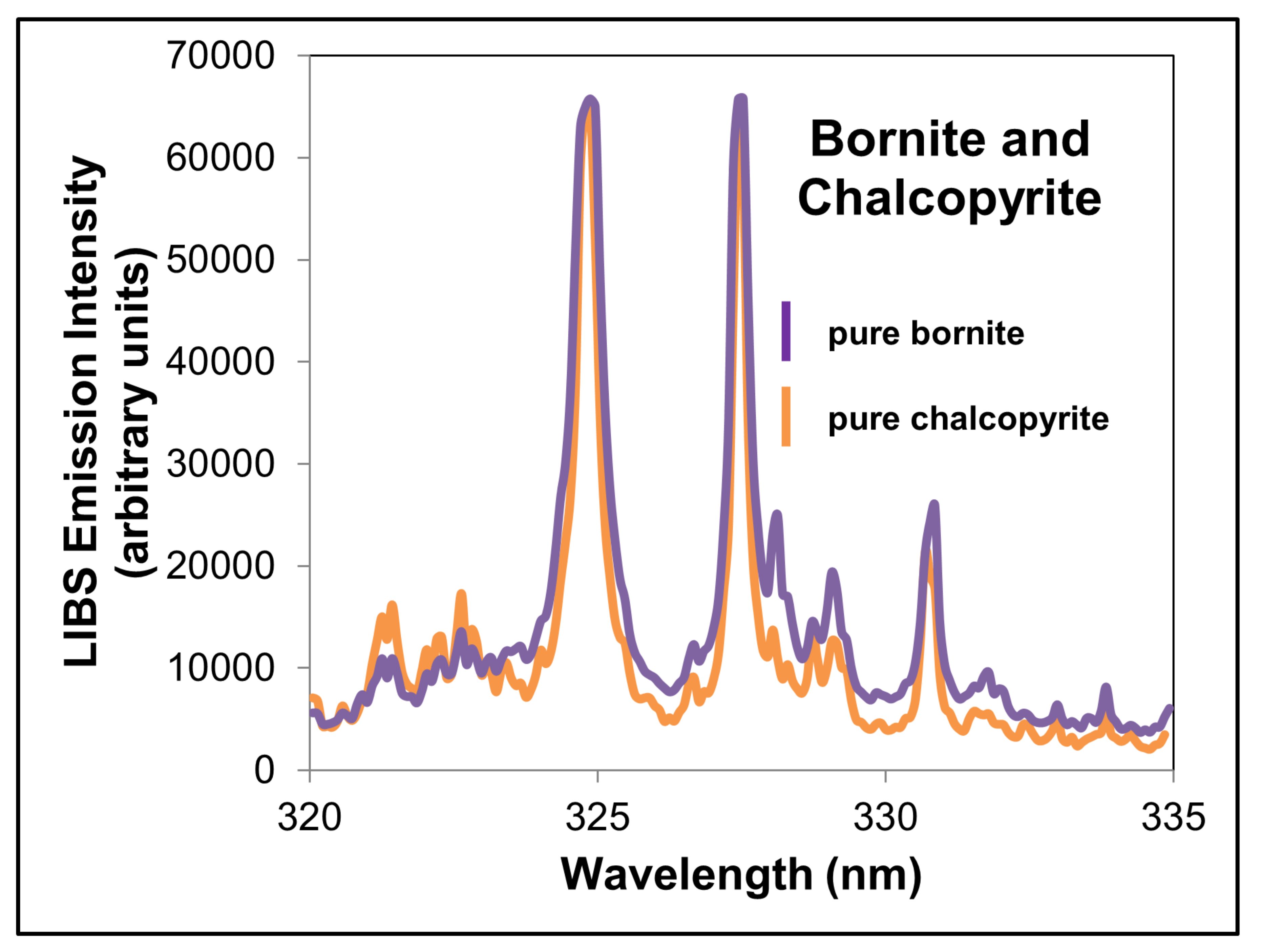
| Integration Intervals and Values | Chalcopyrite | Bornite | Combined Cu-Sulfides |
|---|---|---|---|
| Mineral integration interval 1 (nm) | 324.62–325.13 | 324.62–325.13 | 324.62–325.13 |
| Mineral integration interval 2 (nm) | 327.19–327.70 | 327.19–327.70 | 327.19–327.70 |
| Background integration interval (nm) | 329.6–330.18 | 329.67–330.18 | 329.67–330.18 |
| Pure mineral integration value 1 | 26,239.92 | 29,919.83 | - |
| Pure mineral integration value 2 | 21,116.59 | 24,962.61 | - |
| Pure mineral background integration value (same interval used for 1 and 2) | 2156.21 | 3159.25 | - |
© 2019 by the authors. Licensee MDPI, Basel, Switzerland. This article is an open access article distributed under the terms and conditions of the Creative Commons Attribution (CC BY) license (http://creativecommons.org/licenses/by/4.0/).
Share and Cite
Harmon, R.S.; Lawley, C.J.M.; Watts, J.; Harraden, C.L.; Somers, A.M.; Hark, R.R. Laser-Induced Breakdown Spectroscopy—An Emerging Analytical Tool for Mineral Exploration. Minerals 2019, 9, 718. https://0-doi-org.brum.beds.ac.uk/10.3390/min9120718
Harmon RS, Lawley CJM, Watts J, Harraden CL, Somers AM, Hark RR. Laser-Induced Breakdown Spectroscopy—An Emerging Analytical Tool for Mineral Exploration. Minerals. 2019; 9(12):718. https://0-doi-org.brum.beds.ac.uk/10.3390/min9120718
Chicago/Turabian StyleHarmon, Russell S., Christopher J.M. Lawley, Jordan Watts, Cassady L. Harraden, Andrew M. Somers, and Richard R. Hark. 2019. "Laser-Induced Breakdown Spectroscopy—An Emerging Analytical Tool for Mineral Exploration" Minerals 9, no. 12: 718. https://0-doi-org.brum.beds.ac.uk/10.3390/min9120718