
Minor Contribution by Biomineralizing Phytoplankton to Surface Ocean Biomineral Pools in the Late Stratified Period


National Oceanography Centre, Southampton SO14 3ZH, UK
Oceans 2021, 2(3), 489-508; https://0-doi-org.brum.beds.ac.uk/10.3390/oceans2030028
Submission received: 9 February 2021
/
Revised: 2 July 2021
/
Accepted: 14 July 2021
/
Published: 21 July 2021
Abstract
:Vertical distributions of biogenic silica (bSi), particulate inorganic carbon (PIC) and key biomineral-forming phytoplankton indicate vertical zoning, or partitioning, during the late summer stratified period in the northeast Atlantic. Coccolithophores were generally more numerous in the surface mixed layer, whilst PIC concentrations were more homogenous with depth throughout the euphotic zone. Diatoms were notably more abundant and more diverse in the lower euphotic zone beneath the mixed layer in association with subsurface maxima in chlorophyll-a, bSi and oxygen concentrations. The four dominant coccolithophore species (Emiliania huxleyi, Gephyrocapsa muellerae, Syracosphera spp., and Rhabdosphaera clavigera) represented 78 ± 20% (range 31–100%) of the observed community across all sampled depths yet simultaneously contributed an average of only 13% to measured PIC pools. The diatom community, which was dominated by Pseudo-nitzschia spp. and by a species tentatively identified as Nanoneis longta, represented only ~1% of the bSi pool on average, with contributions increasing within the chlorophyll maximum. Despite a slow gradual deepening of the surface mixed layer in the period prior to observation, and adequate nutrient availability beneath the mixed layer, biomineral pools at this time consisted largely of detrital rather than cellular material.
1. Introduction
Biomineral-forming phytoplankton play an important role in mediating the flux of organic carbon to the ocean’s interior [1,2,3,4]. Bloom-forming taxa such as diatoms and coccolithophores precipitate significant quantities of biogenic silica (bSi) or particulate inorganic carbon (PIC; calcite) throughout the year but particularly during bloom events [5,6,7,8,9]. These biominerals can increase particle density and aid the export of organic material from the upper ocean, with PIC generally considered to be the more important biomineral for sinking fluxes, owing to its greater density [10,11]. In temperate and higher latitude regions of the ocean, coccolithophores typically dominate the phytoplankton community in late spring or summer [12]. In contrast, diatoms are recognized for their dominance during the spring bloom, for their persistence in stratified environments throughout the year [13], and for their contribution to occasional autumn export fluxes [14].
Many studies have demonstrated that different phytoplankton species exhibit preferences for different ecological niches, with strong vertical gradients or temporal changes in environmental conditions being key determinants for when and where species may be found, e.g., [15,16,17]. For the northeast Atlantic, vertical partitioning of phytoplankton groups has been demonstrated both within the seasonal subsurface chlorophyll-a maximum [18], and more generally across the euphotic zone [19], with such partitioning linked to irradiance and nutrient gradients. Nevertheless, information on the co-distribution of inorganic biomineral pools and biomineralizing phytoplankton remains rather limited, particularly for the late stratified period. It is, for example, unclear how relationships found in spring between biomineral and biomineralizing phytoplankton distributions evolve throughout the stratified period (e.g., [20]) or, more simply, whether biomineral pools during the late stratified period are best considered as aged detrital material retained within the upper ocean or as recently produced cellular material, thereby retaining some diagnostic value for recent productivity events. This latter distinction is relevant for understanding the dynamics of remotely sensed PIC pools [21,22], or for identifying the source of ballast material aiding autumn export events, particularly given the significant interannual variability in autumn phytoplankton blooms across the northeast Atlantic [23,24]. Here, biomineral and biomineralizing phytoplankton distributions are examined during the autumn period to quantify and attribute contributions from cellular and detrital material to measured biomineral pools as a step towards improved understanding of biomineral drivers of autumn export events.
2. Materials and Methods
2.1. Sampling and Environmental Characterisation
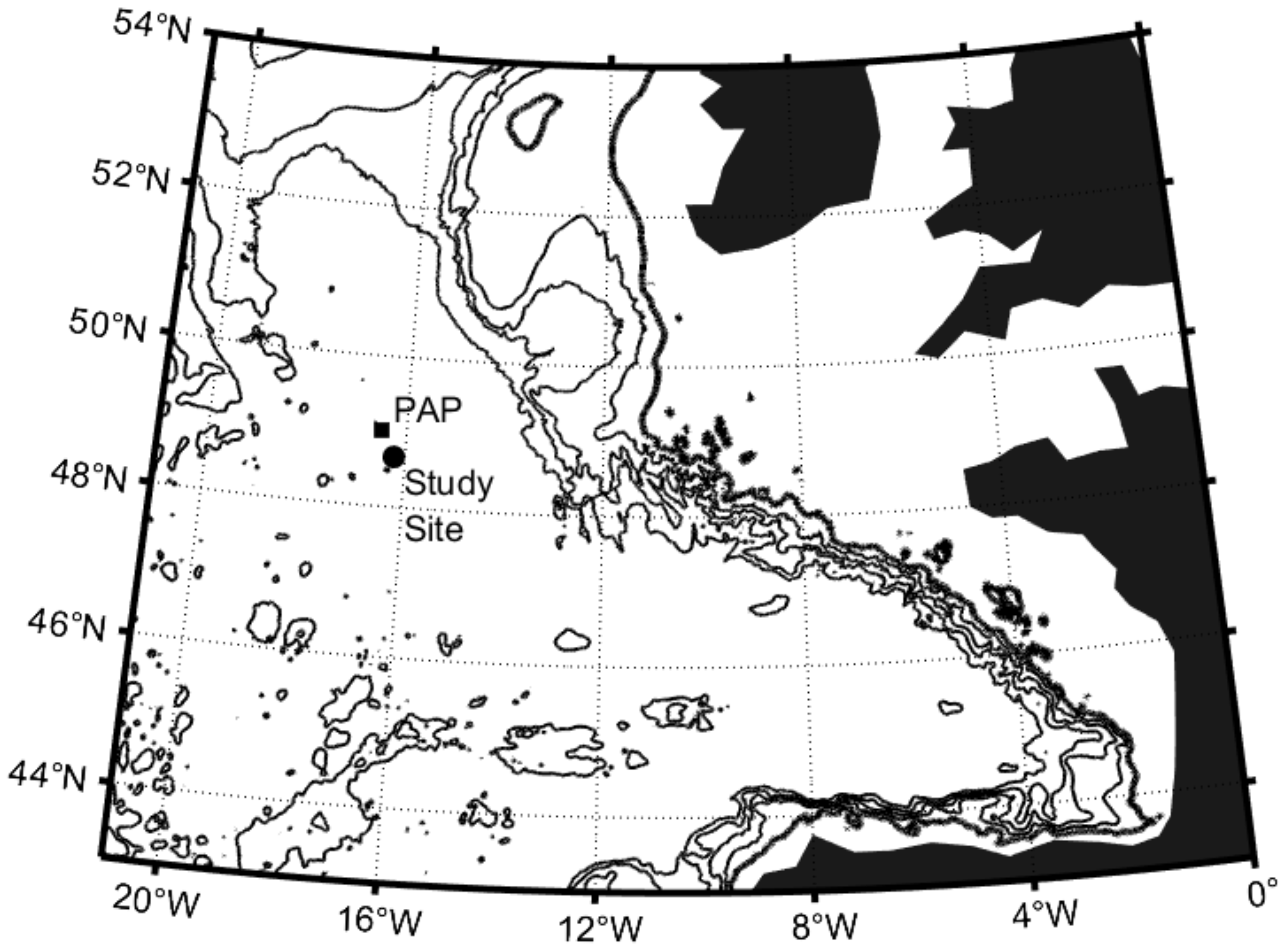
Sampling was conducted in the northeast Atlantic between 3 and 14 September 2013 (early meteorological autumn) at a nominal position of 16.22° W, 48.66° N and approximately 44 km southeast of the Porcupine Abyssal Plain (PAP) sustained observatory (16.5° W, 49° N, Figure 1; [25,26]). The sampling location was the site of an extensive year-long mooring and glider deployment conducted for the OSMOSIS project [27,28], with the cruise itself focused on the recovery of multiple moorings and ocean gliders following conclusion of the OSMOSIS project [29]. CTD operations (Sea-Bird 9/11+; Sea-Bird Electronics Inc., Bellevue, WA, USA) were thus conducted for mooring and glider calibration purposes or to characterise the upper water column for associated turbulent microstructure measurements, with collection of water samples for other purposes a low priority. Results presented here are based on opportunistic water sampling over that 10-day period, with station position dictated by mooring location, glider recovery position or convenience. All stations were located within a 6 km radius of the nominal sampling position, thus providing limited spatial coverage. Water samples were collected from three irradiance layers corresponding to the mixed layer, the lower euphotic zone (base of mixed layer to 1% surface irradiance) and the sub-euphotic zone (<1% surface irradiance to a maximum of ~100 m). Sampling density varied by parameter, with 12 depths sampled between the surface and 100 m for inorganic nutrients, 6 depths for chlorophyll and biominerals pools (~2 depths per irradiance layer) and 3 depths for phytoplankton (1 depth per irradiance layer). Accompanying CTD data were used to estimate the mixed layer depth using the density threshold approach of de Boyer Montegut et al. [30], which identifies the mixed layer depth based on a density increase of 0.03 kg m−3 relative to density at 10 m depth. Profiles of chlorophyll fluorescence and dissolved oxygen concentration were used to provide an indication of biological productivity. Dissolved oxygen concentrations were measured using a Sea-Bird Electronics SBE43 dissolved oxygen sensor (Sea-Bird Electronics Inc., Bellevue, WA, USA) fitted to the CTD frame and calibrated against Winkler titrations. Chlorophyll fluorescence was measured using a Chelsea Technologies AquaTracker (Mk III) fluorometer (Chelsea Technologies Ltd., Surrey, UK) subsequently calibrated against discrete chlorophyll samples.
2.2. Irradiance Conditions
A small number of vertical irradiance (PAR) profiles were obtained (n = 3) and a mean attenuation coefficient (kd) of 0.1007 ± 0.0005 m−1 was calculated from the slope of the natural log of irradiance against depth (e.g., [31]). A mean euphotic depth (Zeu) of 46 m (1% surface irradiance) was estimated from the relationship between optical depth (τ, equivalent to 4.605 for 1% irradiance) and attenuation coefficient (i.e., ).
Subsurface PAR irradiance conditions at selected depths were approximated using the mean attenuation coefficient and surface PAR irradiance measurements (E0) collected using duplicate Skye Instruments PAR sensors (Skye Instruments Ltd., Powys, UK) fitted to the bridge top. Subsurface PAR intensity was estimated using Equation (1) by scaling individual 30 s average E0 measurements with a transmission coefficient of 0.98 [32] to represent transmission through the atmosphere–ocean boundary before PAR at the depth of interest (Ez) was calculated for each time step.
Total daily photon flux (mols photons m−2 d−1) was estimated by summation of all measurements factoring in the 30 s sampling period, whilst maximum daily photon flux (μmols photons m−2 s−1) was taken as the instantaneous daily maximum.
2.3. Nutrients
Concentrations of phosphate, silicate, nitrite and total nitrate (NO3 + NO2) were measured on water samples collected by CTD cast and frozen at −20 °C until analysis. All samples were stored in 15 mL polypropylene falcon tubes and analysed within 1 month of the cruise ending using a SEAL Analytical Quaatro autoanalyzer (SEAL Analytical Ltd., Wrexham, UK) and standard methodologies [33]. Detection limits were estimated as 3 times the standard deviation of the lowest measured standard and were 0.01 for nitrate, 0.03 for silicate and 0.01 for phosphate. Nutrient concentrations are reported in units of μmol L−1.
2.4. Total and Size-Fractionated Chlorophyll-a
Total and size-fractionated chlorophyll-a concentrations (chl-a; mg m−3) were measured fluorometrically using the non-acidified technique of Welschmeyer [34]. For measurements of total chl-a, 250 mL of seawater was filtered through a 25 mm Whatman GF/F filter (Cytiva, Buckinghamshire, UK) followed by pigment extraction in 90% acetone in the dark at 4 °C for 18–20 h. Pigment extracts were measured on a Turner Designs Trilogy fluorometer (Turner Designs, San Jose, CA, USA) calibrated against a pure chl-a standard (Merck, Gillingham, UK).
Size-fractionated chl-a measurements were obtained for two size fractions (>10 μm and <10 μm) by filtering 250 mL of seawater through a 25 mm diameter, 10 μm polycarbonate filter (>10 μm fraction; Whatman Nucleopore (Cytiva, Buckinghamshire, UK)), retaining the filtrate, and filtering this through a 25 mm Whatman GF/F filter (<10 μm fraction (Cytiva, Buckinghamshire, UK)). Pigment extraction and sample analysis for both polycarbonate and GF/F filters followed the procedure for total chl-a measurements.
2.5. Biogenic Silica
Biogenic silica (bSi; μmol L−1) concentrations were obtained following chemical digestion [35]. The 500 mL seawater samples were filtered onto 25 mm diameter 0.8 μm polycarbonate filters (Whatman Nucleopore (Cytiva, Buckinghamshire, UK)). Filters and blanks (fresh filters washed with 0.2 μm filtered seawater) were oven dried at 40 °C and then stored in 15 mL centrifuge tubes. Samples were subsequently digested by the addition of 5 mL of 0.2 M NaOH (Merck, Gillingham, UK) and baked at 85 °C for 2 h before the solution was pH neutralised to pH 7–8, with the addition of 10 mL of 0.1 M HCl (Merck, Gillingham, UK). The solution was then analysed as for dissolved silicate concentrations using a SEAL Analytical Quaatro nutrient autoanalyzer and the same methodologies.
2.6. Particulate Inorganic Carbon
Particulate Inorganic Carbon (PIC; μmol L−1) concentrations were measured using Inductively Coupled Plasma Atomic Mass Spectrometry (ICP-MS) [36]. The 500 mL seawater samples were filtered onto 25 mm diameter 0.8 μm polycarbonate filters (Whatman Nucleopore, (Cytiva, Buckinghamshire, UK)). Residual sea salt was removed by rinsing with a weak analytical grade ammonium solution (180 μL concentrated ammonium hydroxide to 1 L of milli-Q water) and filters were dried at 40 °C and stored in 2 mL Eppendorf tubes until analysis. Filters were transferred to 15 mL Falcon tubes and weighed before being chemically digested in 10 mL of 2% nitric acid and reweighed to obtain the acid weight. Solutions were analysed for calcium content using ICP-MS. The sample inorganic carbon content was derived assuming a 1:1 molar equivalence with the measured calcium content (present as CaCO3).
2.7. Phytoplankton Community
Water samples were collected at 6 stations primarily for analysis of the coccolithophore community. At these stations, between 500 mL and 1 L of seawater was collected by CTD cast from 3 depths and filtered onto 25 mm diameter 0.8 μm polycarbonate filters (Whatman Nucleopore), which were washed with a weak ammonium solution to remove sea salts before being oven dried and stored in labelled petrislides. Sampled depths corresponded to the surface mixed layer, the lower euphotic zone and sub-euphotic zone. A small section (~0.5 × 0.5 cm in dimension) of each filter was mounted onto an aluminium stub and coated in 2 nm gold. A Leo 1450VP scanning electron microscope (SEM) (Carl-Zeiss, Oberkochen, Germany) was used to capture 225 fields of view (FOV) arranged in a 15 × 15 grid covering ~1 mm2 of the filter at a magnification of x5000. The actual volume of seawater examined per sample, taking into account the initial filtered volume and the number of usable FOV, equated to between 1.57 and 3.20 mL. Each FOV micrograph was visually inspected and the coccolithophore species were identified using classification schemes [37,38,39] and enumerated before abundances calculated as
where C is the total number of cells counted, F is the total filter area covered by the sample (mm2), A is the total filter area examined (mm2), and V is the sample volume filtered (mL). A is calculated as the area of each FOV (4.054 × 10⁻³ mm2) multiplied by the number of usable FOV [40].
For interpretative purposes, all Syracosphaera species were aggregated, whilst all other rare coccolithophore species contributing <5% to total community abundance were grouped under the heading of ‘others’.
2.8. Biomineral Budgets
The proportion of the PIC pool represented by dominant coccolithophore taxa was estimated by converting cellular abundances to cellular calcite using established conversion factors [45,46,47] (Table 1). Similarly, the proportion of the bSi pool represented by dominant diatom taxa was estimated using conversion criteria from [48,49,50], specifically 0.12 pmol Si cell−1 for Pseudo-nitzschia sp. (based on P. delicatissima) and 0.02 pmol Si cell−1 for Nanoneis sp. (based on biovolume relationships [49,51]).
3. Results
3.1. Mixed Layer Conditions
The mixed layer depth varied from 20.9 to 34.8 m and, on average, the mixed layer occupied 62% of the euphotic zone (mean depth 46 m; Figure 2). Mean mixed layer conditions for each station are presented in Table 2. Chl-a, bSi and PIC concentrations within the mixed layer were low but variable, suggesting a degree of biological heterogeneity or patchiness within the mixed layer, possibly explained by coincident hydrographic variability (Figure 3). Size-fractionated chl-a data showed that the <10 μm size fraction (i.e., pico- and small nanoplankton) was dominant and represented 90 ± 4% of the total chl-a pool within the mixed layer (Table 2). Nutrient pools were exhausted with mixed layer nutrient concentrations generally <0.1 μmol L−1, though mixed layer Si concentrations did reach 0.2–0.3 μmol L−1 at stations 7 and 8 (Table 2)
3.2. Lower Euphotic Zone
Chlorophyll-a fluorescence profiles revealed the presence of a subsurface chlorophyll maximum within the lower 5% of the euphotic zone (Figure 2). The fluorescence maximum had an average depth of 37.5 ± 4.9 m (range 29.9–43.7 m) (Table 3). The fluorescence maximum was consistently at least 10 m deeper than the base of the mixed layer. Irradiance conditions at the subsurface chlorophyll maximum can only be approximated given the limited number of PAR profiles but the subsurface chlorophyll maximum was found at a depth equivalent to a mean irradiance of 2.6 ± 1.4% (range 1.2 to 4.9%) of surface irradiances. During the study period, the subsurface chlorophyll maximum would have received a daily integrated photon flux of 0.4 to 0.9 mols photons m−2 d−1, with maximum daily photon fluxes of 26 to 48 μmols photons m−2 s−1.
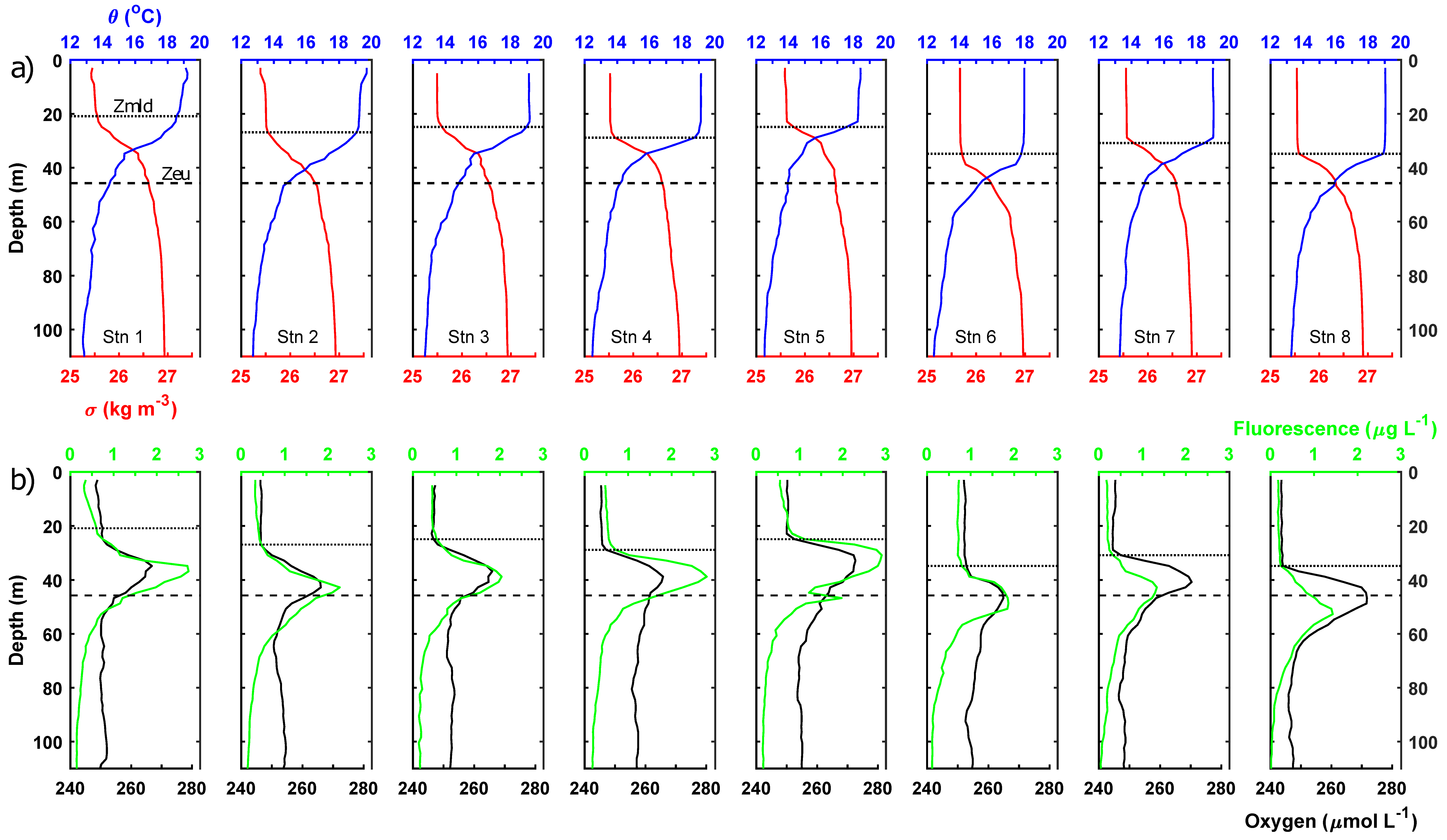
The subsurface chlorophyll maximum was co-located with a subsurface oxygen maximum (Figure 2). Mean mixed layer oxygen concentrations ranged from 243.6 to 252.3 (mean 247.2 ± 2.8) μmol L−1, whilst oxygen concentrations at the subsurface maximum were 265–273 (mean 267.6 ± 3.0) μmol L−1. Oxygen concentrations were, thus, 13–28 (mean 20.4 ± 4.7) μmol L−1 higher at the subsurface oxygen maximum than in the overlying mixed layer. Mean mixed layer oxygen concentrations were ~12.8 μmol L−1 above saturated concentrations at the mean mixed layer temperature and salinities.
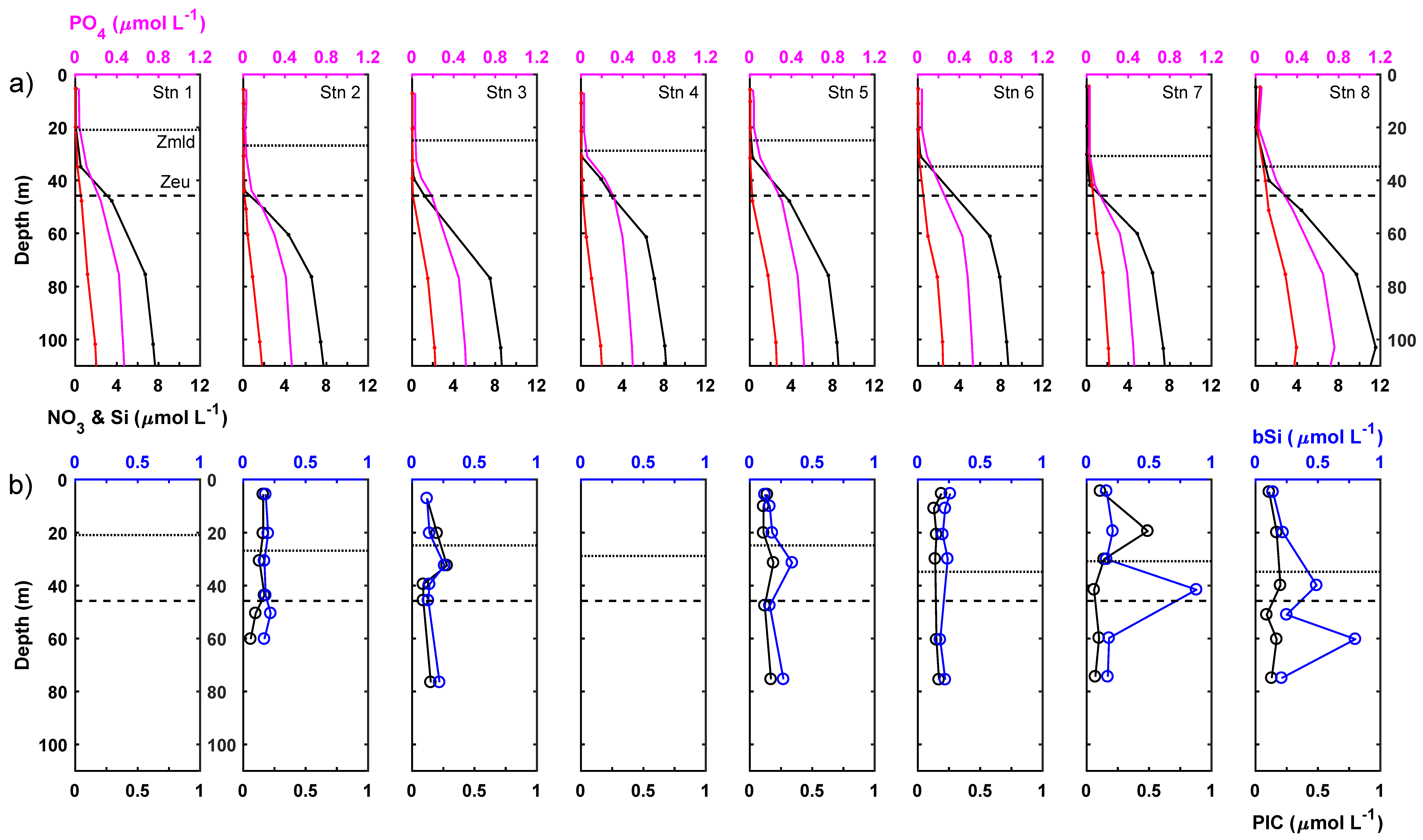
At the subsurface chlorophyll, maximum measured chl-a concentrations were 2.9-fold higher on average than mixed layer chl-a concentrations (Table 3; t-test, p < 0.05). The chl-a pool was still dominated by small phytoplankton <10 μm in size, with this size fraction representing 92 ± 3% of the total chl-a pool. Most stations displayed a very slight shift towards greater dominance of the total chl-a pool by the <10 μm fraction within the lower euphotic zone. Though by no means eutrophic, the subsurface chlorophyll maximum was present in nutrient-replete waters and average macronutrient concentrations were 14.6-fold, 3.2-fold and 2.6-fold higher for NO3− + NO2−, PO43− and Si, respectively, compared to the mixed layer and, thus, comparable to 8%, 20% and 10% of typical winter surface concentrations. NO2− concentrations were occasionally measurable at the subsurface chlorophyll maximum. A midwater bSi maximum was observed in the lower euphotic zone coincident with the subsurface chlorophyll maximum. For individual stations, bSi concentrations could be up to twice as high as measured in the mixed layer, reaching a maximum of 0.52 μmol L−1. On average, bSi concentrations for the lower euphotic zone were around 80% higher than found in the mixed layer. Average PIC concentrations for the lower euphotic zone, meanwhile, were highly comparable to concentrations for the mixed layer, being ~10% lower on average, with limited evidence for any significant vertical gradients. Notably, station 3 did exhibit a PIC peak on the upper shoulder of the chlorophyll maximum (but not at the maximum), whilst station 7 displayed a strong maximum in the mixed layer, indicating vertical heterogeneity (Figure 3).
3.3. Sub-Euphotic Zone
A distinct NO2− maximum was present ~7 m beneath the base of the euphotic zone at a mean depth of 53 ± 7 m equivalent to an average irradiance of 0.6 ± 0.3% (Table 4). The NO2− maximum was ~12 m deeper on average than the subsurface chlorophyll maximum and thus, vertically decoupled from it. Maximum NO2− concentrations reached 0.84 μmol L−1. Chl-a concentrations remained measurable beneath the base of the euphotic zone but decreased rapidly, reaching concentrations of ~0.1 mg m−3 by 75 m. Chl-a concentrations at the NO2− maximum were reduced by around 40% compared to the lower euphotic zone (t-test, p < 0.05) but remained high compared to the surface mixed layer. Mean bSi and PIC concentrations at the NO2− maximum decreased by around 25% compared to concentrations within the lower euphotic zone and decreased further beneath the NO2− maximum.
The nitracline, which could only be approximated from the low-resolution bottle samples, was not correlated consistently to either the depth of the mixed layer or to the depth of the euphotic zone; consequently, both approximations remain valid generic descriptors. Attempts to universally describe the position of the nitracline following linear interpolation and use of either an arbitrary concentration of 0.1 μmol NO3− L−1 or by calculation of the maximum vertical NO3− gradient were also inconsistent. For approximately half of the profiles, the depth of the euphotic zone was equivalent to the depth of maximum NO3− gradient and the euphotic zone depth would, thus, seem to be the most common shorthand description for the position of the nitracline.
3.4. Integrated Results
Nutrient, particulate and chlorophyll-a pools were uniformly integrated to 50 m to summarise conditions for the euphotic zone (Table 5). Integrated nutrient pools varied 5.9-fold for NO3−, 2.6-fold for PO43− and 13-fold for Si between stations, whereas integrated total chl-a varied only 1.8-fold. There was slightly more variability in the >10 μm chl-a size fraction, which varied 2.8-fold between stations. Integrated bSi and PIC pools varied 2.2-fold and 1.4-fold between stations, with averages of 11.7 ± 3.5 mmol Si m−2 and ~8.1 ± 1.1 mmol C m−2. Integrated bSi concentrations were significantly correlated with integrated Si concentrations (Integrated bSi = 0.243 × Integrated Si + 8.4316 (R2 = 0.76, p < 0.05)), whereas integrated bSi and mixed layer or surface bSi concentrations were not significantly correlated.
3.5. Phytoplankton Community
A total of 50 phytoplankton species were identified from the SEM micrographs, consisting of 27 coccolithophores, 2 silicoflagellates, 10 dinoflagellates and 11 diatoms.
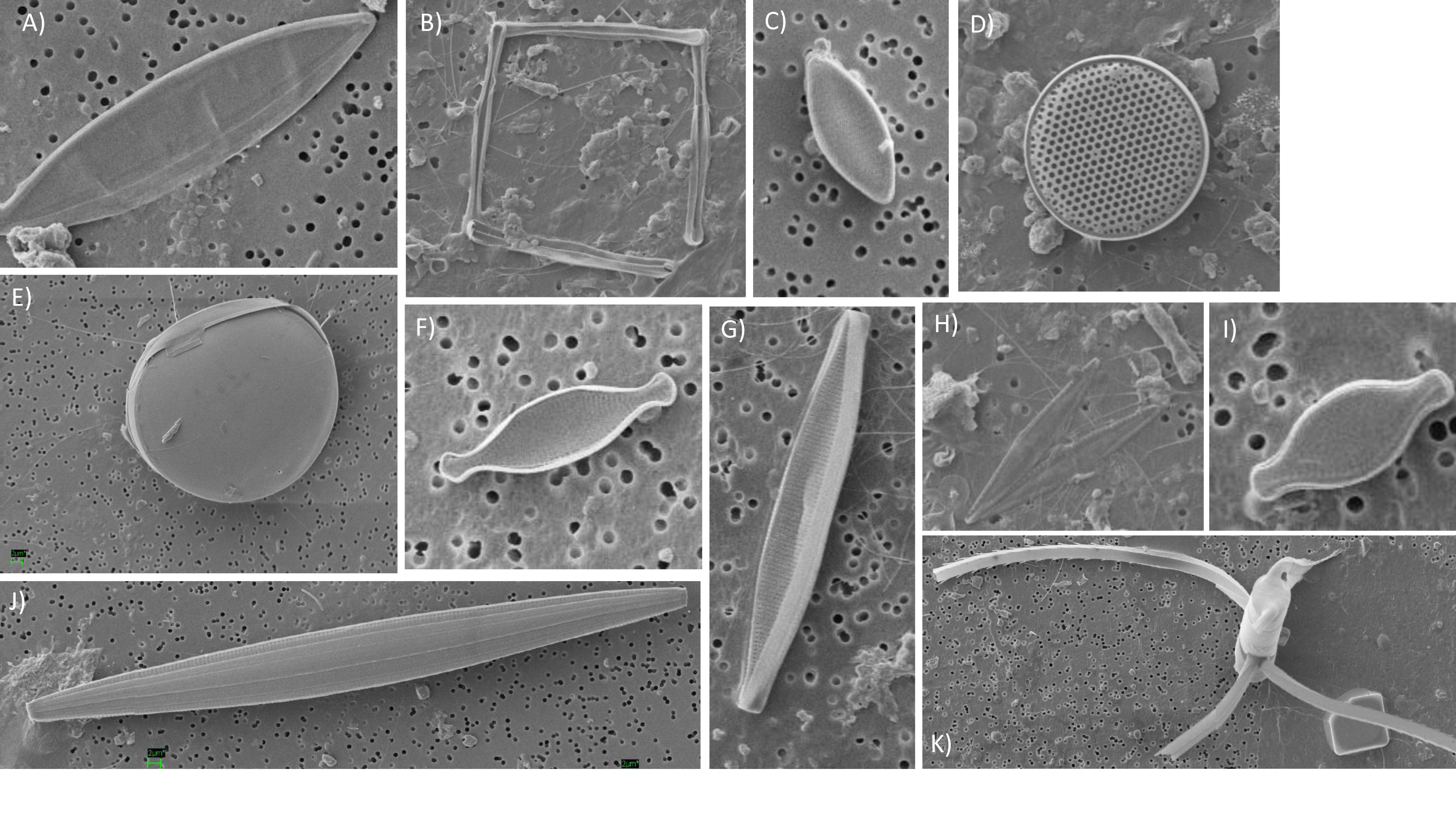
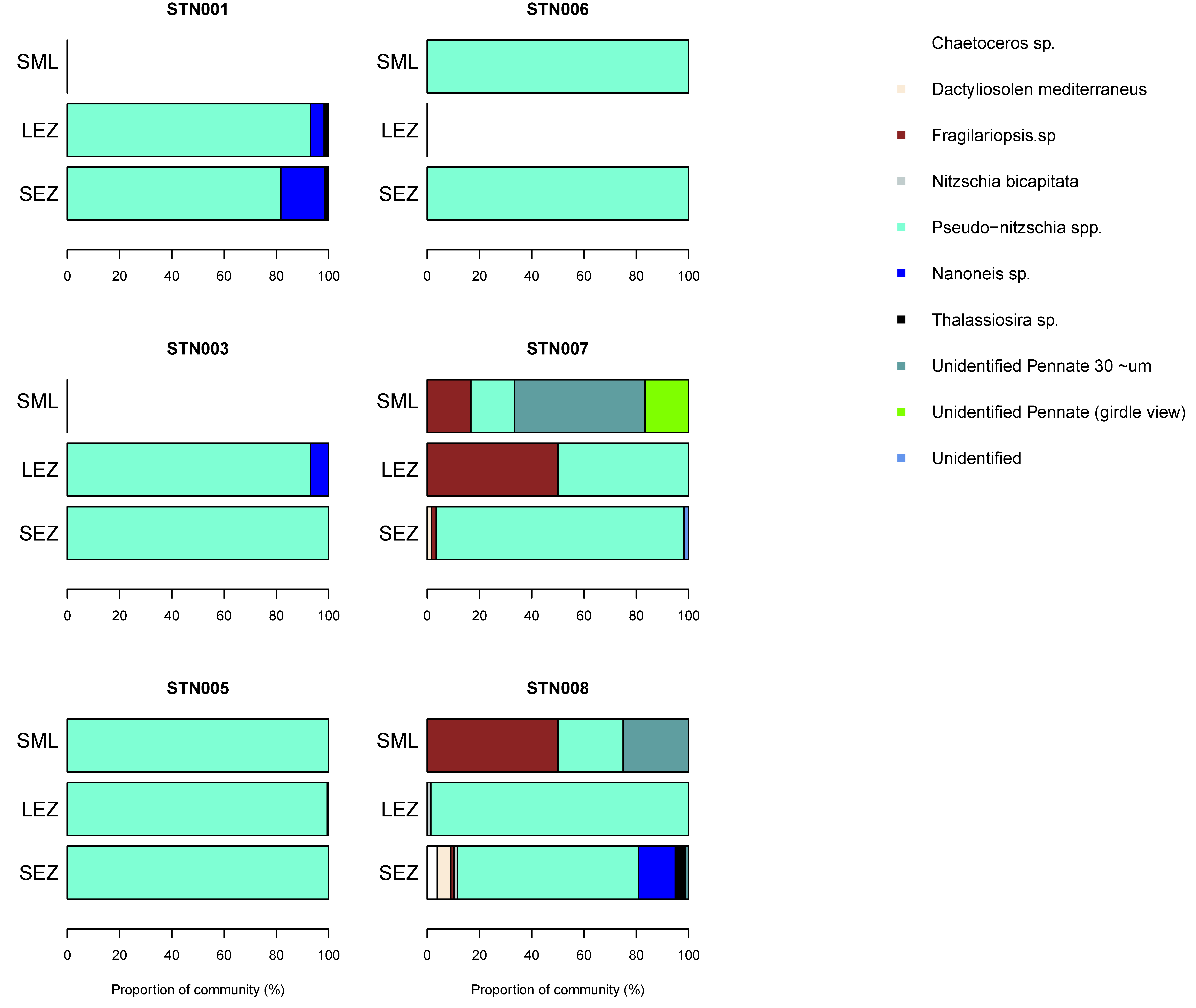
Diatom diversity was low in the surface mixed layer (four species) but increased to eight species within the lower euphotic zone. Pseudo-nitzschia spp. (delicatissima group; width <3 μm) were common to most samples (up to 110 cells mL−1). Infrequent observations of a species tentatively identified as Nanoneis longta (up to 9.9 cells mL−1), Chaetoceros sp. (one sample; 1.8 cells mL−1), Dactyliosolen mediterraneus (two samples, up to 2.5 cells mL−1) and Thalassiosira sp. (three samples, up to 1.8 cells mL−1) were also made (Figure 4). Small Pseudo-nitzschia spp. cells (<20 μm in length) were dominant, representing on average 78% of observed diatom cells, occasionally being the only diatom genus present (Figure 5). Mean abundances of Pseudo-nitzschia spp. were low in the surface mixed layer (0.4 ± 0.4 cells mL−1) but increased in the lower euphotic zone (34.6 ± 33.6 cells mL−1) and sub-euphotic zone (38.9 ± 8.5 cells mL−1). Mean abundances of Nanoneis longta displayed a comparable vertical distribution, increasing from 0 cells mL−1 in the surface mixed layer to 0.5 ± 0.9 cells mL−1 in the lower euphotic layer and 5.6 ± 5.1 cells mL−1 in waters immediately below the base of the euphotic zone.
The silicoflagellates Dictyocha fibula (<0.63 cells mL−1) and Dictyocha speculum (<0.62 cells mL−1) were rarely observed and only within the lower euphotic zone.
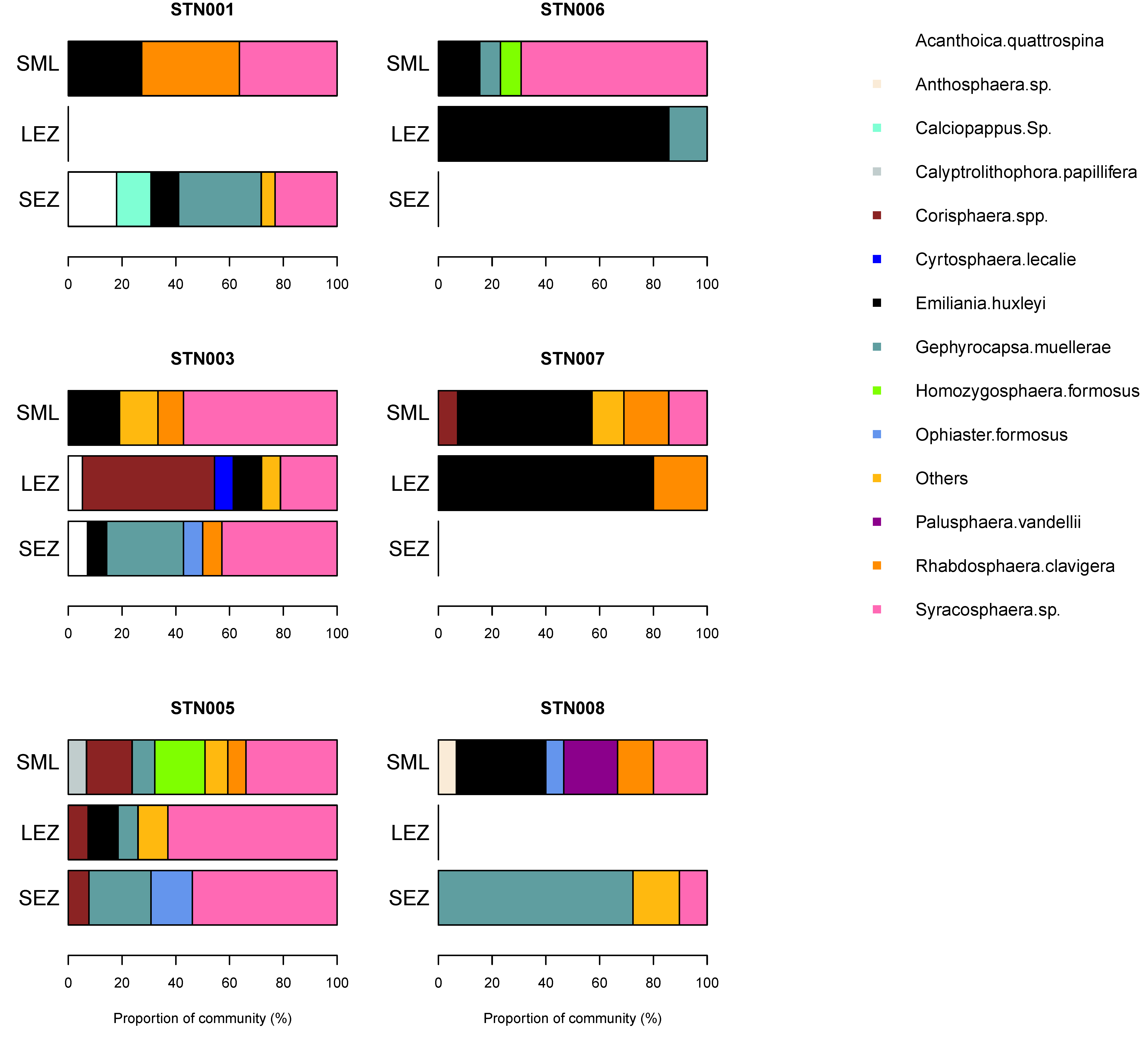
Coccolithophore diversity was highest in the surface mixed layer (4–12 species per sample) but a second diversity peak (7–11 species) was also present in the lower euphotic zone coincident with the subsurface chlorophyll maximum. Common coccolithophore species were Emiliania huxleyi (up to 13.2 cells mL−1), Gephyrocapsa muellerae (13.1 cells mL−1), Rhabdosphaera clavigera (4.4 cells mL−1), and Syracosphera spp. (10.8 cells mL−1). The coccolithophore community varied significantly between stations and between sampled depths, suggesting a heterogenous environment. Viewed as a proportion of the coccolithophore community, the cosmopolitan species Emiliania huxleyi could represent up to 85% of the community in an individual sample (Figure 6). Notable contributions from Gephyrocapsa muellerae (up to 72%), Syracosphera spp. (up to 69%), Corisphaera spp. (up to 49%) and Rhabdosphaera clavigera (up to 36%) were also evident within individual samples. All other species made maximum contributions of <20%. Samples representing the lower euphotic zone displayed frequent changes in the dominant species, suggesting extensive patchiness in this depth interval. Corisphaera spp. was present at three stations, notably station 3, where it represented a major component (49%) of the community in the lower euphotic zone, and station 5, where it was present at all sampled depths (surface mixed layer, lower euphotic zone and sub-euphotic zone), but, elsewhere, was otherwise rare (<17% of community). On average, Emiliania huxleyi, Gephyrocapsa muellerae, Syracosphera spp., and Rhabdosphaera clavigera represented 78 ± 20% (range 31–100%) of the observed community across all sampled depths.
There were strong vertical gradients in species abundance for several species. The mean abundance of E. huxleyi decreased from 4.2 ± 4.7 cells mL−1 in the surface mixed layer to 1.1 ± 1.5 cells mL−1 in the lower euphotic zone. The gradient in R. clavigera mean abundances was similar, decreasing sharply, with depth from a maximum of 1.4 ± 1.5 cells mL−1 in the surface mixed layer, whilst Syracosphera spp. abundances were largely invariant, with depth ranging from 2.8 to 3.8 cells mL−1. Amongst the four dominant species, G. muellerae was the only species to show an increase in mean abundance with depth, with highest average abundances of 6.2 ± 6.0 cells mL−1 found in waters technically beneath the base of the euphotic zone.
3.6. PIC Budget
Contributions made by individual coccolithophore species to measured PIC pools varied widely between samples but were generally rather small. For the entire dataset, Emiliania huxleyi accounted for an average of only 1.1 ± 1.7% (range 0 to 6.5%) of measured PIC pools. An identical contribution of 1.1 ± 0.9% (range 0 to 2.8%) was made by Syracosphaera spp. Larger contributions of 2.5 ± 5.9% (range 0 to 23.4%) were made by Gephyrocapsa mullerae, whilst Rhabdosphaera clavigera contributed 8.2 ± 14.5% (range 0 to 56.1%). Collectively, these four species accounted for an average of 12.9 ± 16.3% (range 0 to 64.1%) of measured PIC pools. Vertically, however, there were some notable gradients. On average, E. huxleyi represented 1.9 ± 2.6% of the mixed layer PIC pool, 0.7 ± 0.8% of the lower euphotic zone PIC pool and 0.2 ± 0.3% of the sub-euphotic zone pool, suggesting a vertical partitioning of the species distribution given otherwise stable PIC concentrations between the mixed layer and lower euphotic zone. A similar pattern was evident for R. clavigera, which represented 19.5 ± 21.4%, 4.1 ± 4.7% and 0% of the mixed layer, lower euphotic zone and sub-euphotic zone PIC pools, respectively. G. mullerae displayed a marked contrasting pattern contributing 0.6 ± 0.7%, 1.3 ± 1.8% and 12.9 ± 14.8% of the mixed layer, lower euphotic zone and sub-euphotic zone PIC pools, respectively, and thus, made greater contributions to PIC pools with increased depth. The contribution made by Syracosphaera spp. displayed no clear vertical gradient, with mean contributions of 1.6 ± 0.8%, 0.7 ± 1.0% and 1.2 ± 0.4% for the mixed layer, lower euphotic zone and sub-euphotic zone PIC pools.
3.7. bSi Budget
Although small Pseudo-nitzschia sp. and Nanoneis longta dominated the diatom community, they appear to have contributed very little to the bSi pool. Pseudo-nitzschia sp. accounted for an average of 1.0 ± 1.2% (range 0 to 3.9%) of individual bSi samples, whilst N. longta accounted for an average of 0.01 ± 0.02% (range 0 to 0.05%). Collectively, these two genera accounted for an average of 1.0 ± 1.2% (range 0 to 3.9%) of the measured bSi pool. Vertically, Pseudo-nitzschia sp. represented an average of 0.04 ± 0.03% of the mixed layer bSi pool, 1.5 ± 1.4% of the lower euphotic zone bSi pool and 2.1 ± 0.69% of the sub-euphotic zone pool. N. longta, meanwhile, represented ~0.0 ± 0%, 0.01 ± 0.01% and 0.03 ± 0.04%, respectively. Both species represented more of the bSi pool with depth, but neither were dominant components.
4. Discussion
Biomineralizing plankton make important contributions to carbon export fluxes via the addition of mineral ballast to particulate organic carbon [1]. In temperate waters with marked seasonality such contributions are usually greatest during, or immediately following, periods of high biomineral synthesis such as during blooms, or following the onset of seasonal mixing (the so-called ‘fall dump’ [14]). The observations reported here indicate vertical zoning in the respective distributions of PIC, bSi and biomineral-forming phytoplankton throughout the euphotic zone during the stratified conditions typical of the late summer/early autumn period. Diatoms, in particular, were more diverse and more numerous in the lower euphotic zone beneath the mixed layer, coincident with a subsurface chlorophyll-a maximum, a bSi maximum and an oxygen maximum, with these co-located features implying active biological production. These results are consistent with previous observations from the northeast Atlantic region, indicating primary production occurring at depth during the summer months [52,53] and with reports of diatom pigment markers beneath the mixed layer [19]. In contrast, coccolithophores were typically more abundant within the surface mixed layer, whilst PIC concentrations were more homogenous with depth throughout the euphotic zone. Previous descriptions of the vertical distribution of coccolithophores and diatoms in the northeast Atlantic under stratified conditions indicated that both groups were more likely to be located at depth particularly in association with a subsurface chlorophyll maximum [18]. Such observations only partially agree with results presented here, whilst diatoms were indeed found to be associated with the subsurface chlorophyll maximum—a clear preference for the mixed layer was evident for coccolithophore species.
Conditions in surface waters were nutrient-poor, with an indication that NO3− may have been more strongly drawn down than P or Si. Compared to typical winter nutrient concentrations, which, for this region of the northeast Atlantic, are ~8, ~0.5 and ~3 μmol L−1 for NO3−, PO43−, and Si [54,55,56,57], the mean surface concentrations represented <1, 6 and 3% of typical winter concentrations for NO3−, PO43−, and Si, respectively. Such conditions, therefore, may not be favourable for high rates of production. Typical winter nutrient concentrations were reached at around 120 m depth.
Integrated PIC and bSi concentrations were comparable to previous observations reported for this time of year (e.g., [6,19]), suggesting that the observed distributions may be broadly typical for the northeast Atlantic region. Significantly, neither the observed coccolithophore nor diatom species were found to make substantial and sustained contributions to measured biomineral pools, with the low cellular contributions confirming that the bulk of both PIC and bSi pools consisted of detrital material. Though, how robust are such conclusions?
In this study, cellular abundances have been used to estimate the proportion of the PIC or bSi pool represented by cellular material by using estimates of cellular PIC or Si content as conversion factors. Implicitly, therefore, the misidentification of species or use of inappropriate estimates of the cellular elemental content would have an impact on the budgetary calculations. As diatom diversity was lower than the coccolithophore diversity, any such errors are likely more significant for the bSi budget than for the PIC budget but both budgets contain important caveats.
In the case of the PIC budget, the presence of rare heavily calcified coccolithophore species, and of other calcifying organisms, may distort the overall cellular contribution [45], though this is considered unlikely in this case, as not only were significant quantities of detrital material visually evident in individual SEM micrographs but even loose coccoliths from rarer, more heavily calcified species (e.g., Calcidiscus leptoporus) were only very infrequently observed (though not completely absent). Thus, the low contribution of 13% made by the four dominant coccolithophore taxa (E. huxleyi, G. muellerae, Syracosphera spp., and R. clavigera) to the PIC pool of the temperate northeast Atlantic (48.7° N) contrasts markedly with comparable observations reported from the Iceland Basin (59–60° N), where during late summer non-bloom conditions, Emiliania huxleyi alone can represent 68–89% of the PIC pool [58]. This difference likely reflects the diverse environments sampled (temperate vs. sub-polar) and the significant latitudinal gradient in coccolithophore distribution and abundance present in this part of the North Atlantic [12,20,59].
For the bSi budget, the estimate of the bSi pool represented by diatom cells indicated a low cellular contribution of ~1%. This estimate is biased by the assumption that the two dominant diatom species were the only species contributing to the bSi pool, whilst any contribution from silicoflagellates was minimal. Furthermore, diatom abundances and community diversity may have been underestimated as a consequence of enumerating from small seawater volumes (<3.2 mL). Nevertheless, for seven of the eight stations, the assumption that Pseudo-nitzschia spp. and N. longta were dominant appears correct, whilst omission of rarer species from the bSi budgetary calculations is unlikely to significantly impact the overall conclusion that the bSi pool was predominately detrital in character. At station 8, a notably different diatom community was encountered, which included several larger species including Chaetoceros sp. and Dactyliosolen mediterraneus, indicating spatial patchiness may also be an important caveat on the low estimate of cellular contribution.
Due to the low diversity of species, correct identification of those species represents a critical constraint on the bSi budget. Cells identified in this study as Pseudo-nitzschia sp. could not be identified to the species level due to low image resolution obscuring taxonomic details, thus introducing some uncertainty over both species identity and the most appropriate cellular Si conversion factor to use. Several independent taxonomic experts were consulted but were unable to reach a consensus on identity. Based on knowledge of the phytoplankton community at the sampling location and for the time of year (e.g., [60]), cells were attributed (by the author) to the Pseudo-nitzschia genus. Cells were subsequently associated with the delicatissima group/complex by virtue of having widths <3 μm and a linear shape, (e.g., [42,61]). A cellular Si content of 0.12 pmol Si cell−1 was thus assumed based on the results of Boutorh et al. [50] for Pseudo-nitzschia delicatissima. This cellular Si content is for nutrient- and iron-replete conditions. Under Fe-depleted conditions, the cellular Si content can halve to 0.06 μmol Si cell−1 [50]. A caveat to the bSi budgetary calculations, therefore, is that the estimated contribution by Pseudo-nitzschia cells to the bSi pool could have been approximately 50% lower were Fe limitation present in the northeast Atlantic at the time of sample collection. This reduction would not, however, invalidate the general conclusion that the bSi pool was predominantly detrital.
More fundamental, however, are concerns over the accuracy of the cellular Si content used in the calculations to derive the bSi budget. The typical length of Pseudo-nitzschia delicatissima cells (40–76 um; [42]) is generally longer than for the cells observed here (~15–30 μm), potentially indicating an overestimation of the contribution made by these smaller Pseudo-nitzschia cells to the bSi pool (if similarly silicified). Again, such a situation would not alter the general conclusion that the bSi pool is predominantly detrital. However, at 0.12 pmol Si cell−1, the Si content is towards the lower end of estimates for other species within this genus. For example, Marchetti and Harrison [62] reported cellular Si contents of between 0.57 and 2.69 pmol cell−1 for four Pseudo-nitzschia species (P. heimii (type 1), P. heimeii (type 2), P. dolorosa, P. turgidula) under Fe replete conditions. Notably, such estimates imply cellular Si contents that are ~5 to ~22 times larger than assumed here. Translated to the bSi budget calculations, such increases would have a significant impact on the estimate of the bSi pool represented by Pseudo-nitzschia cells (potentially increasing that contribution to 22%). However, P. heimii is a comparatively large cell (typical length 67–120 um) [42] and more usually considered part of the Pseudo-nitzschia seriata group [42], so use of its cellular Si content of 2.69 pmol cell−1 is not appropriate here. The estimate of 0.57 pmol Si cell−1 reported by Marchetti and Harrison [62] for P. dolorosa, however, may be a viable alternative (based solely on affiliation with the delicatissima group), with the implication that, on average, ~4.8% of the bSi pool could be represented by Pseudo-nitzschia. Whilst this would represent a significant increase from the 1% contribution estimated here, the majority of the bSi pool nonetheless remains detrital.
Implications for Autumn Export Events
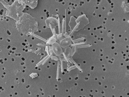
Small diatoms within the nanoplankton size class (2–20 μm) are generally overlooked due to the difficulties of identification, but may play an important role in carbon export fluxes [63]. In the northeast Atlantic, observations of Nanoneis are limited to reports of Nanoneis hasleae, a small 5 μm cell, occurring during the spring bloom [64,65]. In the Gulf of Mexico, however, high subsurface abundances of the larger N. longta have been reported during late summer and early autumn [66]. Although the resolution of the micrograph shown in Figure 4b precludes visualization of all key taxonomic characteristics to definitively identify the cells as N. longta, the colony morphology and timing of the observation are comparable to examples reported by recent studies [66,67]. Furthermore, at ~18 μm in length, the individual cells appear larger than the standard description of N. hasleae [42,68], potentially making this a rare observation of N. longta in the northeast Atlantic.
At the time of sampling, the seasonal breakdown of stratification had yet to commence, mixed layer chlorophyll and nutrient concentrations were low, and the chlorophyll pool (and by extension the phytoplankton community) was dominated by small cells <10 μm in size. Continuous mixed layer depth measurements reported by [28], however, show that the mixed layer had approximately doubled in thickness from its annual minimum depth of ~15 m measured in July to the average depth of 27 m reported here for September. Despite this deepening, the mean mixed layer conditions reported in this study remained comparable to the summer seasonal means reported by [28]. Consequently, the observed distribution of biominerals and phytoplankton likely represented conditions prior to any autumn export pulse. Partial support for this statement is provided by long-term sediment trap records collected at 3000 m depth at the PAP site northwest of the study region [69] (Figure 1), which registered a small peak in dry-weight flux in mid-October, approximately 1 month later [70]. Assuming an approximate sinking velocity of ~100 m day−1 for sinking particles [71], organic material ballasted with biomineral material may have begun to exit the upper ocean at approximately the same time as observed here. Thus, the results presented here imply that detrital biomineral material, potentially accumulated in surface waters throughout the summer period, is likely more important for aiding autumnal export pulses rather than cellular biomineral material resulting from in situ growth.
Funding
Cruise JC090 was conducted in support of the OSMOSIS (Ocean Surface Mixing, Ocean Sub-mesoscale Interaction Study) project funded by NERC (Natural Environment Research Council) grant NE/1020083/1 (split award NE/I01993X/1). Additional funding was provided by the EU Framework 7 project EuroBASIN (FP7-ENV-2010) and NERC National Capability.
Data Availability Statement
Data reported in this study are available via the British Oceanographic Data Centre; www.bodc.ac.uk (accessed on 2 July 2021).
Acknowledgments
Anna Rumyantseva, Emily Trill, David Marshall and Madeleine Youngs are thanked for opportunistic sample collection; Mark Stinchcombe (nutrients) and Richard Pearce (SEM management) are thanked for assistance with sample analyses.
Conflicts of Interest
The author declares no conflict of interest. The funders had no role in the design of the study; in the collection, analyses, or interpretation of data; in the writing of the manuscript, or in the decision to publish the results.
References
- Klass, C.; Archer, D.E. Association of sinking organic matter with various types of mineral ballast in the deep sea: Implications for the rain ratio. Glob. Biogeochem. Cycles 2002, 16, 1116. [Google Scholar] [CrossRef]
- Passow, U.; De La Rocha, C.L. Accumulation of mineral ballast on organic aggregates. Glob. Biogeochem. Cycles 2006, 20, GB1013. [Google Scholar] [CrossRef] [Green Version]
- Sanders, R.; Morris, P.J.; Poulton, A.J.; Stinchcombe, M.C.; Charalampopoulou, A.; Lucas, M.I.; Thomalla, S.J. Does a ballast effect occur in the surface ocean? Geophys. Res. Lett. 2010, 37, L08602. [Google Scholar] [CrossRef] [Green Version]
- Le Moigne, F.A.C.; Sanders, R.J.; Villa-Alfageme, M.; Martin, A.P.; Pabortsava, K.; Planquette, H.; Morris, P.J.; Thomalla, S.J. On the proportion of ballast versus non-ballast associated carbon export in the surface ocean. Geophys. Res. Lett. 2012, 39, L15610. [Google Scholar] [CrossRef] [Green Version]
- Paasche, E.; Ostergren, I. The annual cycle of plankton diatom growth and silica production in the inner Oslofjord. Limnol. Oceanogr. 1980, 25, 481–494. [Google Scholar]
- Leblanc, K.; Leynaert, A.; Fernandez, I.C.; Rimmelin, P.; Moutin, T.; Raimbault, P.; Ras, J.; Queguiner, B. A seasonal study of diatom dynamics in the North Atlantic during the POMME experiment (2001): Evidence for Si limitation of the spring bloom. J. Geophys. Res. 2005, 110, C07S14. [Google Scholar] [CrossRef] [Green Version]
- Terrats, L.; Claustre, H.; Cornec, M.; Magin, A.; Neukermans, G. Detection of Coccolithophore Blooms with BioGeoChemical-Argo Floats. Geophys. Res. Lett. 2020, 47, e2020GL090559. [Google Scholar] [CrossRef]
- O’Brien, C.J.; Peloquin, J.A.; Vogt, M.; Heinle, M.; Gruber, N.; Ajani, P.; Andruleit, H.; Arıstegui, J.; Beaufort, L.; Estrada, M.; et al. Global marine plankton functional type biomass distributions: Coccolithophores. Earth Syst. Sci. Data 2013, 5, 259–276. [Google Scholar] [CrossRef] [Green Version]
- Leblanc, K.; Arıstegui, J.; Armand, L.; Assmy, P.; Beker, B.; Bode, A.; Breton, E.; Cornet, V.; Gibson, J.; Gosselin, M.-P.; et al. A global diatom database—abundance, biovolume and bimass in the world ocean. Earth Syst. Sci. Data 2012, 4, 149–165. [Google Scholar] [CrossRef] [Green Version]
- Francois, R.; Honjo, S.; Krishfield, R.; Manganini, S. Factors controlling the flux of organic carbon to the bathypelagic zone of the ocean. Glob. Biogeochem. Cycles 2002, 16, 1087. [Google Scholar] [CrossRef] [Green Version]
- Rings, A.; Lücke, A.; Schleser, G.H. A new method for the quantitative separation of diatom frustules from lake sediments. Limnol. Oceanogr. Methods 2004, 2, 25–34. [Google Scholar] [CrossRef]
- Hopkins, J.; Henson, S.A.; Painter, S.C.; Tyrrell, T.; Poulton, A.J. Phenological characteristics of global coccolithophore blooms. Glob. Biogeochem. Cycles 2015, 29, 239–253. [Google Scholar] [CrossRef] [Green Version]
- Kemp, A.E.S.; Villareal, T.A. The case of the diatoms and the muddled mandalas: Time to recognize diatom adaptations to stratified waters. Prog. Oceanogr. 2018, 167, 138–149. [Google Scholar] [CrossRef]
- Kemp, A.E.S.; Pike, J.; Pearce, R.B.; Lange, C.B. The “fall dump”—A new pespective on the role of a "shade flora" in the annual cycle of diatom production and export flux. Deep Sea Res. Part II 2000, 47, 2129–2154. [Google Scholar] [CrossRef]
- Caracciolo, M.; Beaigrand, G.; Helaouet, P.; Gevaert, F.; Edwards, M.; Lizon, F.; Kleparski, L.; Goberville, E. Annual phytoplankton succession results from niche-environment interaction. J. Plankton Res. 2020, 43, 85–102. [Google Scholar] [CrossRef]
- Brun, P.; Vogt, M.; Payne, M.R.; Gruber, N.; O’Brien, C.J.; Buitenhuis, E.T.; Le Quere, C.; Leblanc, K.; Luo, Y.-W. Ecological niches of open ocean phytoplankton taxa. Limnol. Oceanogr. 2015, 60, 1020–1038. [Google Scholar] [CrossRef] [Green Version]
- Boyd, P.W.; Strzepek, R.; Fu, F.; Hutchins, D.A. Environmental control of open-ocean phytoplankton groups: Now and in the future. Limnol. Oceanogr. 2010, 55, 1353–1376. [Google Scholar] [CrossRef]
- Latasa, M.; Cabello, A.M.; Moran, X.A.G.; Massana, R.; Scharek, R. Distribution of phytoplankton groups within the deep chlorophyll maximum. Limnol. Oceanogr. 2017, 62, 665–685. [Google Scholar] [CrossRef] [Green Version]
- Painter, S.C.; Finlay, M.; Hemsley, V.S.; Martin, A.P. Seasonality, phytoplankton succession and the biogeochemical impacts of an autumn storm in the northeast Atlantic Ocean. Prog. Oceanogr. 2016, 142, 72–104. [Google Scholar] [CrossRef] [Green Version]
- Leblanc, K.; Hare, C.E.; Feng, Y.; Berg, G.M.; DiTullio, G.R.; Neely, A.; Benner, I.; Sprengel, C.; Beck, A.; Sanudo-Wilhelmy, S.A.; et al. Distribution of calcifying and silicifying phytoplankton in relation to environmental and biogeochemical parameters during the late stages of the 2005 North East Atlantic Spring Bloom. Biogeosciences 2009, 6, 2155–2179. [Google Scholar]
- Gordon, H.R.; Bynton, G.C.; Balch, W.M.; Groom, S.B.; Harbour, D.S.; Smyth, T.J. Retrieval of coccolithophore calcite concentration from SeaWiFS imagery. Geophys. Res. Lett. 2001, 28, 1587–1590. [Google Scholar] [CrossRef]
- Balch, W.M.; Gordon, H.R.; Bowler, B.C.; Drapeau, D.T.; Booth, E.S. Calcium carbonate measurements in the surface global ocean based on Moderate-Resolution Imaging Spectroradiometer data. J. Geophys. Res. 2005, 110, C07001. [Google Scholar] [CrossRef]
- Friedland, K.D.; Record, N.R.; Asch, R.G.; Kristiansen, T.; Saba, V.S.; Drinkwater, K.F.; Henson, S.; Leaf, R.T.; Morse, R.E.; Johns, D.G.; et al. Seasonal phytoplankton blooms in the North. Atlantic linked to the overwintering strategies of copepods. Elem. Sci. Anthr. 2016, 4, 000099. [Google Scholar] [CrossRef]
- Martinez, E.; Antoine, D.; D’Ortenzio, F.; de Boyer Montegut, C. Phytoplankton spring and fall blooms in the North Atlantic in the 1980s and 2000s. J. Geophys. Res. 2011, 116, C11. [Google Scholar] [CrossRef] [Green Version]
- Lampitt, R.S.; Billet, D.S.M.; Martin, A.P. The sustained observatory over the Porcupine Abyssal Plain (PAP): Insights from time series observations and process studies. Deep. Sea Res. Part II 2010, 57, 1267–1271. [Google Scholar] [CrossRef]
- Hartman, S.E.; Bett, B.J.; Durden, J.M.; Henson, S.A.; Iversen, M.; Jeffreys, R.M.; Horton, T.; Lampitt, R.; Gates, A.R. Enduring science: Three decades of observing the Northeast Atlantic from the Porcupine Abyssal Plain Sustained Observatory (PAP-SO). Prog. Oceanogr. 2021, 191, 102508. [Google Scholar] [CrossRef]
- Buckingham, C.E.; Naveira-Garabato, A.C.; Thompson, A.F.; Brannigan, L.; Lazar, A.; Marshall, D.P.; Nurser, A.J.G.; Damerell, G.; Heywood, K.J.; Belcher, S.E. Seasonality of submesoscale flows in the ocean surface boundary layer. Geophys. Res. Lett. 2016, 43, 2118–2126. [Google Scholar] [CrossRef] [Green Version]
- Damerell, G.M.; Heywood, K.J.; Calvert, D.; Grant, A.L.M.; Bell, M.J.; Belcher, S.E. A comparison of five surface mixed layer models with a year of observations in the North Atlantic. Prog. Oceanogr. 2020, 187, 102316. [Google Scholar] [CrossRef]
- Naveira-Garabato, A. Cruise Report: RRS James Cook Cruise 090, 30 August–17 September 2013. Ocean Surface Mixing, Ocean Sub-Mesoscale Interaction Study (OSMOSIS); National Oceanography Centre: Southampton, UK, 2013; 111p. [Google Scholar]
- de Boyer Montegut, C.; Madec, G.; Fischer, A.S.; Lazar, A.; Ludicone, D. Mixed layer depth over the global ocean: An. examination of profile data and a profile-based climatology. J. Geophys. Res. 2004, 109, C12003. [Google Scholar] [CrossRef]
- Lee, Z.-P.; Du, K.-P.; Arnone, R. A model for the diffuse attenuation coefficient of downwelling irradiance. J. Geophys. Res. 2005, 110. [Google Scholar] [CrossRef]
- Kirk, J.T.O. Light and Photosynthesis in Aquatic Ecosystem, 3rd ed.; Cambridge University Press: Cambridge, UK, 2010. [Google Scholar]
- Hydes, D.J.; Aoyama, M.; Aminot, A.; Bakker, K.; Becker, S.; Coverly, S.; Daniel, A.; Dickson, A.G.; Grosso, O.; Kerouel, R.; et al. Determination of dissolved nutrients (N, P, Si) in seawater with high precision and inter-comparability using gas-segmented continuous flow analysers. In The GO-Ship Repeat Hydrography Manual: A Collection of Expert Reports and Guidelines; Hood, E.M., Sabine, C.L., Sloyan, B.M., Eds.; IOCCP Report No. 14, ICPO Publication Series No. 134; ICPO: Paris, France, 2010; pp. 1–87. Available online: http://www.ioccp.org/images/06Nutrients/Hydes_et_al_Nutrients.pdf (accessed on 16 July 2021).
- Welschmeyer, N.A. Fluorometric analysis of chlorophyll a in the presence of chlorophyll b and phaeopigments. Limnol. Oceanogr. 1994, 39, 1985–1992. [Google Scholar] [CrossRef]
- Ragueneau, O.; Treguer, P. Determination of biogenic silica in coastal waters: Applicability and limits of the alkaline digestion method. Marine Chem. 1994, 45, 43–51. [Google Scholar] [CrossRef]
- Green, D.R.H.; Cooper, M.J.; German, C.R.; Wilson, P.A. Optimization of an inductively coupled plasma—Optical emission spectrometry method for the rapid determination of high-precision Mg/Ca and Sr/Ca in foraminiferal calcite. Geochem. Geophys. Geosyst. 2003, 4, 8404. [Google Scholar] [CrossRef]
- Cros, L.; Fortuno, J.-M. Atlas of Northwestern Mediterranean coccolithophores. Sci. Mar. 2002, 66, 1–186. [Google Scholar] [CrossRef] [Green Version]
- Young, J.; Geisen, M.; Cros, L.; Kleijne, A.; Sprengel, C.; Probert, I.; Østergaard, J. A guide to extant coccolithophore taxonomy. J. Nannoplankton Res. Spec. Issue 2003, 1, 1–125. [Google Scholar]
- Nannotax3. Available online: www.mikrotax.org/Nannotax3/ (accessed on 16 July 2021).
- Charalampopoulou, A.; Poulton, A.J.; Tyrrell, T.; Lucas, M.I. Irradiance and pH affect coccolithophore community composition on a transect between the North Sea and the Arctic Ocean. Mar. Ecol. Prog. Ser. 2011, 431, 25–43. [Google Scholar] [CrossRef] [Green Version]
- Poulton, A.J.; Holligan, P.M.; Charalampopoulou, A.; Adey, T.R. Coccolithophore ecology in the tropical and subtropical Atlantic Ocean: New perspectives from the Atlantic meridional transect (AMT) programme. Prog. Oceanogr. 2017, 158, 150–170. [Google Scholar] [CrossRef]
- Hasle, G.R.; Syvertsen, E.E. Marine diatoms. In Identifying Marine Phytoplankton; Tomas, C.R., Ed.; Academic Press: San Diego, CA, USA, 1997; pp. 5–385. [Google Scholar]
- Round, F.E.; Crawford, R.M.; Mann, D.G. The Diatoms: Biology and Morphology of the Genera; Cambridge University Press: Cambridge, UK, 1990; p. 747. [Google Scholar]
- Steidinger, K.A.; Tangen, K. Dinoflagellates. In Identifying Marine Phytoplankton; Tomas, C.R., Ed.; Academic Press: San Diego, CA, USA, 1997; pp. 387–584. [Google Scholar]
- Daniels, C.J.; Poulton, A.J.; Young, J.R.; Esposito, M.; Humphreys, M.P.; Ribas-Ribas, M.; Tynan, E.; Tyrrell, T. Species-specific calcite production reveals Coccolithus pelagicus as the key calcifier in the Arctic Ocean. Mar. Ecol. Prog. Ser. 2016, 555, 29–47. [Google Scholar] [CrossRef] [Green Version]
- Young, J.R.; Ziveri, P. Calculation of coccolith volume and its use in calibration of carbonate flux estimates. Deep Sea Res. Part II 2000, 47, 1679–1700. [Google Scholar] [CrossRef]
- Yang, T.-N.; Wei, K.-Y. How many coccoliths are there in a coccosphere of the extant coccolithophorids? A compilation. J. Nannoplankton Res. 2003, 25, 7–15. [Google Scholar]
- Brzezinski, M.A. The Si:C:N ratio of marine diatoms: Interspecific variability and the effect of some environmental variables. J. Phycol. 1985, 21, 347–357. [Google Scholar] [CrossRef]
- Conley, D.J.; Kilham, S.S.; Theriot, E. Differences in silica content between marine and freshwater diatoms. Limnol. Oceanogr. 1989, 34, 205–213. [Google Scholar] [CrossRef] [Green Version]
- Boutorh, J.; Moriceau, B.; Gallinari, M.; Ragueneau, O.; Bucciarelli, E. Effect of trace metal-limited growth on the postmortem dissolution of the marine diatom Pseudo-nitzschia delicatissima. Glob. Biogeochem. Cycles 2016, 30, 57–69. [Google Scholar] [CrossRef]
- Hillebrand, H.; Durselen, C.-D.; Kirschtel, D.; Pollingher, U.; Zohary, T. Biovolume calculations for pelagic and benthic microalgae. J. Phycol. 1999, 35, 403–424. [Google Scholar] [CrossRef]
- Hemsley, V.S.; Smyth, T.J.; Martin, A.P.; Frajka-Williams, E.; Thompson, A.F.; Damerell, G.; Painter, S.C. Estimating oceanic primary production using vertical irradiance and chlorophyll profiles from ocean gliders in the North Atlantic. Environ. Sci. Technol. 2015, 49, 11612–11621. [Google Scholar] [CrossRef] [PubMed] [Green Version]
- Longhurst, A. Seasonal cycles of pelagic production and consumption. Prog. Oceanogr. 1995, 36, 77–167. [Google Scholar] [CrossRef]
- Koeve, W. Wintertime nutrients in the North Atlantic—New approaches and implications for new production estimates. Mar. Chem. 2001, 74, 245–260. [Google Scholar] [CrossRef]
- Hartman, S.E.; Larkin, K.E.; Lampitt, R.S.; Lankhorst, M.; Hydes, D.J. Seasonal and inter-annual biogeochemical variations in the Porcupine Abyssal Plain 2003–2005 associated with winter mixing and surface circulation. Deep Sea Res. Part II 2010, 57, 1303–1312. [Google Scholar] [CrossRef]
- Hartman, S.E.; Jiang, Z.-P.; Turk, D.; Lampitt, R.S.; Frigstad, H.; Ostle, C.; Schuster, U. Biogeochemical variations at the Porcupine Abyssal Plain Sustained Observatory (PAP-SO) in the northeast Atlantic Ocean, from weekly to inter-annual time scales. Biogeosciences 2015, 12, 845–853. [Google Scholar] [CrossRef] [Green Version]
- Boyer, T.P.; Antonov, J.I.; Baranova, O.K.; Coleman, C.; Garcia, H.E.; Grodsky, A.; Johnson, D.R.; Locarnini, R.A.; Mishonov, A.V.; O’Brien, T.D.; et al. World Ocean Database 2013; NOAA Atlas NESDIS 72; Levitus, S., Mishonov, A., Eds.; National Oceanographic Data Center: Silver Spring, MD, USA, 2013; p. 209. [Google Scholar]
- Poulton, A.J.; Charalampopoulou, A.; Young, J.R.; Tarran, G.A.; Lucas, M.I.; Quartly, G.D. Coccolithophore dynamics in non-bloom conditions during late summer in the central Iceland Basin (July–August 2007). Limnol. Oceanogr. 2010, 55, 1601–1613. [Google Scholar] [CrossRef] [Green Version]
- Taylor, A.H.; Harbour, D.S.; Harris, R.P.; Burkill, P.H.; Edwards, E.S. Seasonal succession in the pelagic ecosystem of the North Atlantic and the utilization of nitrogen. J. Plankton Res. 1993, 15, 875–891. [Google Scholar] [CrossRef]
- Continuous Plankton Recorder Survey Team. Continuous Plankton Records: Plankton atlas of the North Atlantic Ocean. Mar. Ecol. Prog. Ser. Suppl. 2004, 11–75. [Google Scholar]
- Fehling, J.; Davidson, K.; Bolch, C.; Tett, P. Seasonality of Pseudo-nitzschia spp. (Bacillariophyceae) in western Scottish waters. Mar. Ecol. Prog. Ser. 2006, 323, 91–105. [Google Scholar] [CrossRef] [Green Version]
- Marchetti, A.; Harrison, P.J. Coupled changes in the cell morphology and the elemental (C, N, and Si) composition of the pennate diatom Pseudo-nitzschia due to iron deficiency. Limnol. Oceanogr. 2007, 52, 2270–2284. [Google Scholar] [CrossRef]
- Leblanc, K.B.; Queguiner, F.; Diaz, V.; Cornet, M.; Michel-Rodriguez, X.; Durrieu de Madron, C.; Bowler, S.; Malviya, M.; Thyssen, G.; Gregori, M.; et al. Nanoplanktonic diatoms are globally overlooked but play a role in spring blooms and carbon export. Nat. Commun. 2018, 9, 953. [Google Scholar] [CrossRef] [PubMed]
- Savidge, G.; Turner, D.R.; Burkill, P.H.; Watson, A.J.; Angel, M.V.; Pingree, R.D.; Leach, H.; Richards, K.J. The BOFS 1990 spring bloom experiment: Temporal evolution and spatial variability of the hydrogrpahic field. Prog. Oceanogr. 1992, 29, 235–281. [Google Scholar] [CrossRef]
- Savidge, G.; Boyd, P.; Pomroy, A.; Harbour, D.; Joint, I. Phytoplankton production and biomass estimates in the northeast Atlantic Ocean, May–June 1990. Deep Sea Res. I 1995, 42, 599–617. [Google Scholar] [CrossRef]
- Nienow, J.A.; Snyder, R.A.; Jeffrey, W.H.; Wise, S. Fine structure and ecology of Nanoneis longta in the northeastern Gulf of Mexico with a revised definition of the species. Diatom Res. 2016, 32, 43–58. [Google Scholar] [CrossRef]
- Villar, E.; Ferrant, G.K.; Follows, M.; Garczarek, L.; Speich, S.; Audic, A.; Bittner, L.; Blanke, B.; Brum, J.R.; Brunet, C.; et al. Environmental characteristics of Agulhas rings affect interocean plankton transport. Science 2015, 348, 1261447. Available online: http://www.igs.cnrs-mrs.fr/Tara_Agulhas/#FigW9 (accessed on 20 May 2021). [CrossRef] [Green Version]
- Norris, R.E. A new planktonic diatom, Nanoneis hasleae gen. et sp. nov. Nor. J. Bot. 1973, 20, 321–325. [Google Scholar]
- Lampitt, R.S.; Salter, I.; de Cuevas, B.A.; Hartman, S.; Larkin, K.E.; Pebody, C.A. Long-term variability of downward particle flux in the deep northeast Atlantic: Causes and trends. Deep Sea Res. Part II 2010, 57, 1346–1361. [Google Scholar] [CrossRef]
- Horton, T.; Thurston, M.H.; Vlierboom, R.; Gutteridge, Z.; Pebodu, C.A.; Gates, A.R.; Bett, B.J. Are abyssal scavenging amphipod assemblages linked to climate cycles? Prog. Oceanogr. 2020, 184, 102318. [Google Scholar] [CrossRef]
- Alldredge, A. Particle Aggregation Dynamics. In Encyclopedia of Ocean Sciences, 2nd ed.; Academic Press: Cambridge, MA, USA, 2001; pp. 330–337. [Google Scholar]
Figure 1.
Study location in the northeast Atlantic with sampling site indicated by the black circle. The nominal position of the Porcupine Abyssal Plain (PAP) sustained observatory is indicated by the black square.
Figure 1.
Study location in the northeast Atlantic with sampling site indicated by the black circle. The nominal position of the Porcupine Abyssal Plain (PAP) sustained observatory is indicated by the black square.

Figure 2.
Vertical profiles of (a) temperature (blue) and density (red) and (b) fluorescence (green) and dissolved oxygen (black). Respective mixed layer depth indicated by solid black horizontal line and average euphotic zone depth indicated by horizontal dashed line in each panel.
Figure 2.
Vertical profiles of (a) temperature (blue) and density (red) and (b) fluorescence (green) and dissolved oxygen (black). Respective mixed layer depth indicated by solid black horizontal line and average euphotic zone depth indicated by horizontal dashed line in each panel.

Figure 3.
Vertical profiles of (a) phosphate (pink), nitrate (black) and silicate (red) and (b) biogenic silica (bSi; blue) and particulate inorganic carbon (PIC; black). Respective mixed layer depth indicated by solid black horizontal line and average euphotic zone depth indicated by horizontal dashed line in each panel.

Figure 4.
Photomontage of observed diatom species. (A) Unidentified pennate 30 μm long, (B) Nanoneis longta, (C) Fragilariopsis sp., (D) Thalassiosira sp., (E) Unidentified, (F) Nitzschia sp., (N. bicapitata?), (G) Navicula sp. ~30 μm, (H) Pseudo-nitzschia sp., (I) Nitzschia bicapitata, (J) Unidentified diatom—girdle view, (K) Chaetoceros sp. Note that images are not to scale.

Figure 5.
Diatom community composition in autumn in the northeast Atlantic. Results are based on cellular abundances and presented by station and by sampled depth corresponding to the surface mixed layer (SML), lower euphotic zone (LEZ) and sub-euphotic zone (SEZ). See text for definitions.
Figure 5.
Diatom community composition in autumn in the northeast Atlantic. Results are based on cellular abundances and presented by station and by sampled depth corresponding to the surface mixed layer (SML), lower euphotic zone (LEZ) and sub-euphotic zone (SEZ). See text for definitions.

Figure 6.
Coccolithophore community composition in autumn in the northeast Atlantic. Results are based on cellular abundances and presented by station and by sampled depth corresponding to the surface mixed layer (SML), lower euphotic zone (LEZ) and sub-euphotic zone (SEZ). See text for definitions.


Table 1.
Coccolithophore cellular conversion factors.
| Species | Coccolith Calcite (pmol) | Coccoliths per Cell | Cellular Calcite (pmol) | Source |
|---|---|---|---|---|
| Emiliania huxleyi | 0.024 | 22 | 0.52 | [45] |
| Syracosphaera spp. | 0.012 | 35 | 0.42 | [45] |
| Gephyrocapsa mullerae | 0.080 | 20 | 1.60 | [46,47] |
| Rhabdosphaera clavigera | 0.67 | 20 | 13.49 | [46,47] |
Table 2.
Sampling locations and mean mixed layer conditions for each station. The proportion (%) of chl-a in the <10 μm size fraction is shown in parentheses in the total chl-a column.
Table 2.
Sampling locations and mean mixed layer conditions for each station. The proportion (%) of chl-a in the <10 μm size fraction is shown in parentheses in the total chl-a column.
| Station | Date/Time | Latitude (° N) | Longitude (° W) | Mixed Layer Depth (m) | Temperature (°C) | Salinity (PSS-78) | Total Chl-a (mg/m3) (% <10 μm) | NO3− (μmol L−1) | PO43− (μmol L−1) | Si (μmol L−1) | bSi (μmol L−1) | PIC (μmol L−1) |
|---|---|---|---|---|---|---|---|---|---|---|---|---|
| 1 | 03/09/2013 15:49 | 48.6802 | 16.1907 | 20.9 | 18.96 | 35.59 | 0.58 (88.4) | 0.04 | 0.04 | 0.02 | - | - |
| 2 | 03/09/2013 19:34 | 48.6802 | 16.1907 | 26.8 | 19.35 | 35.71 | 0.41 (91.6) | 0.03 | 0.03 | 0.05 | 0.19 | 0.16 |
| 3 | 04/09/2013 13:01 | 48.6827 | 16.1590 | 24.9 | 19.12 | 35.66 | 0.67 (90.9) | 0.05 | 0.03 | 0.02 | 0.13 | 0.16 |
| 4 | 04/09/2013 21:39 | 48.6685 | 16.2330 | 28.8 | 19.11 | 35.70 | 0.63 (-) | 0.05 | 0.03 | 0.03 | - | - |
| 5 | 06/09/2013 18:03 | 48.6465 | 16.2605 | 24.9 | 18.33 | 35.55 | 0.73 (85.5) | 0.04 | 0.04 | 0.04 | 0.16 | 0.12 |
| 6 | 08/09/2013 18:38 | 48.7102 | 16.2028 | 34.8 | 17.94 | 35.50 | 0.95 (85.5) | 0.09 | 0.05 | 0.07 | 0.23 | 0.15 |
| 7 | 12/09/2013 15:27 | 48.6282 | 16.2760 | 30.8 | 19.01 | 35.71 | 0.52 (94.4) | 0.04 | 0.03 | 0.23 | 0.17 | 0.25 |
| 8 | 13/09/2013 09:29 | 48.6325 | 16.2728 | 34.8 | 19.03 | 35.70 | 0.51 (92.7) | 0.04 | 0.05 | 0.30 | 0.18 | 0.14 |
| Mean ± S.D. | 28.3 ± 5.0 | 18.9 ± 0.5 | 35.64 ± 0.08 | 0.63 ± 0.17 (89.9 ± 3.5) | 0.05 ± 0.02 | 0.04 ± 0.01 | 0.09 ± 0.11 | 0.15 ± 0.07 | 0.14 ± 0.07 |
Table 3.
Conditions at the subsurface chlorophyll maximum (SCM) taken as representing the lower euphotic zone. The proportion (%) of chl-a in the <10 μm size fraction is shown in parentheses in the total chl-a column.
Table 3.
Conditions at the subsurface chlorophyll maximum (SCM) taken as representing the lower euphotic zone. The proportion (%) of chl-a in the <10 μm size fraction is shown in parentheses in the total chl-a column.
| Station | Depth of SCM (m) | Light Level % | Total Chl-a (mg m−3) (% <10 μm) | NO2 (μmol L−1) | NO3 (μmol L−1) | PO4 (μmol L−1) | Si (μmol L−1) | bSi (μmol L−1) | PIC (μmol L−1) |
|---|---|---|---|---|---|---|---|---|---|
| 1 | 35.0 | 2.9 | 2.85 (91.1) | 0.1 | 0.52 | 0.11 | 0.21 | - | - |
| 2 | 43.7 | 1.2 | 1.30 (93.8) | <LOD | 0.08 | 0.06 | 0.03 | 0.17 | 0.15 |
| 3 | 39.5 | 1.9 | 1.41 (93.9) | 0.1 | 0.46 | 0.11 | 0.06 | 0.17 | 0.15 |
| 4 | 39.3 | 1.9 | 2.01 (-) | 0.1 | 1.00 | 0.15 | 0.09 | - | - |
| 5 | 31.3 | 4.3 | 2.63 (90.4) | <LOD | 0.28 | 0.10 | 0.03 | 0.34 | 0.19 |
| 6 a | 29.9 | 4.9 | 1.43 (85.5) | 0.01 | 0.26 | 0.09 | 0.11 | 0.24 | 0.14 |
| 7 | 41.6 | 1.5 | 0.91 (95.8) | 0.01 | 0.17 | 0.06 | 0.39 | 0.52 | 0.10 |
| 8 | 39.9 | 1.8 | 1.49 (94.1) | 0.24 | 1.31 | 0.20 | 0.96 | 0.49 | 0.20 |
| Mean ± S.D. | 37.5 ± 4.9 | 2.6 ± 1.4 | 1.75 ± 0.68 (92.1 ± 3.4) | 0.09 ± 0.09 | 0.51 ± 0.43 | 0.11 ± 0.05 | 0.23 ± 0.32 | 0.32 ± 0.15 | 0.16 ± 0.04 |
a Note that due to advective movement of the water column between down cast and up cast, results for station 6 (30 m) appear vertically separated from the depth of the fluorescence maximum (49 m) shown in Figure 2.
Table 4.
Conditions at the Primary Nitrite Maximum (PNM) (beneath base of traditional euphotic zone, 1% surface irradiance). The proportion (%) of chl-a in the <10 μm size fraction is shown in parentheses in the total chl-a column.
Table 4.
Conditions at the Primary Nitrite Maximum (PNM) (beneath base of traditional euphotic zone, 1% surface irradiance). The proportion (%) of chl-a in the <10 μm size fraction is shown in parentheses in the total chl-a column.
| Station | Depth of PNM (m) | Light Level % | Total Chl-a (mg m−3) (% <10 μm) | NO2 (μmol L−1) | NO3 (μmol L−1) | PO4 (μmol L−1) | Si (μmol L−1) | bSi (μmol L−1) | PIC (μmol L−1) |
|---|---|---|---|---|---|---|---|---|---|
| 1 | 47.9 | 0.8 | 1.8 (94.7) | 0.71 | 3.57 | 0.25 | 0.61 | - | - |
| 2 | 60.2 | 0.2 | 1.1 (95.1) | 0.84 | 4.35 | 0.3 | 0.42 | 0.20 | 0.08 |
| 3 | 45.6 | 1.0 | 1.3 (94.4) | 0.31 | 1.2 | 0.19 | 0.09 | 0.22 | 0.15 |
| 4 | 61.1 | 0.2 | 0.3 (-) | 0.61 | 6.28 | 0.4 | 0.52 | - | - |
| 5 | 47.5 | 0.8 | 1.1 (93.6) | 0.8 | 3.8 | 0.31 | 0.26 | 0.22 | 0.15 |
| 6 a | - | - | - | - | - | - | - | - | - |
| 7 | 59.8 | 0.2 | 0.8 (-) | 0.31 | 4.87 | 0.32 | 0.98 | 0.18 | 0.09 |
| 8 | 51.0 | 0.6 | 1.3 (98.0) | 0.82 | 4.42 | 0.36 | 1.27 | 0.42 | 0.13 |
| Mean ± S.D. | 53.3 ± 6.8 | 0.6 ± 0.3 | 1.11 ± 0.44 (95.2 ± 1.7) | 0.63 ± 0.23 | 4.07 ± 1.54 | 0.30 ± 0.07 | 0.59 ± 0.41 | 0.25 ± 0.10 | 0.12 ± 0.03 |
a No nitrite maximum observed at station 6.
Table 5.
Euphotic zone (0–50 m) integrated nutrient, particulate and chlorophyll pools.
| Station | Integration Depth (m) | Integrated NO3− (mmol m−2) | Integrated PO43− (mmol m−2) | Integrated Si (mmol m−2) | Integrated bSi (mmol Si m−2) | Integrated PIC (mmol C m−2) | Integrated Total Chl-a (mg m2) | Integrated <10 μm Chl-a (mg m2) | % of Total Chl-a in <10 μm Fraction | Integrated >10 μm Chl-a (mg m2) | % of Total Chl-a in >10 μm Fraction |
|---|---|---|---|---|---|---|---|---|---|---|---|
| 1 | 50 | 39.87 | 4.71 | 8.87 | - | 65.4 | 59.7 | 91.2 | 5.8 | 8.8 | |
| 2 | 50 | 8.01 | 2.33 | 2.48 | 9.16 | 7.64 | 42.1 | 39.3 | 93.6 | 2.7 | 6.4 |
| 3 | 50 | 13.21 | 3.26 | 2.20 | 7.85 | 8.06 | 44.8 | 41.6 | 92.9 | 3.2 | 7.1 |
| 4 | 50 | 39.32 | 5.42 | 3.59 | - | 58.1 | - | - | - | - | |
| 5 | 50 | 44.66 | 5.56 | 4.37 | 10.40 | 7.09 | 67.4 | 60.2 | 89.4 | 7.1 | 10.6 |
| 6 | 50 | 47.50 | 5.26 | 9.24 | 11.35 | 7.51 | 48.8 | 42.0 | 85.9 | 6.9 | 14.1 |
| 7 | 50 | 14.05 | 2.64 | 16.52 | 17.40 | 10.09 | 38.4 | 35.9 | 93.6 | 2.5 | 6.4 |
| 8 | 50 | 40.94 | 5.96 | 28.61 | 14.24 | 7.98 | 45.0 | 42.4 | 94.2 | 2.6 | 5.8 |
| Mean ± S.D. | 30.95 ± 16.20 | 4.39 ± 1.43 | 9.48 ± 9.09 | 11.73 ± 3.52 | 8.06 ± 1.06 | 51.2 ± 11.0 | 45.9 ± 9.9 | 92 ± 3 | 4.4 ± 2.1 | 8 ± 3 |
Publisher’s Note: MDPI stays neutral with regard to jurisdictional claims in published maps and institutional affiliations. |
© 2021 by the author. Licensee MDPI, Basel, Switzerland. This article is an open access article distributed under the terms and conditions of the Creative Commons Attribution (CC BY) license (https://creativecommons.org/licenses/by/4.0/).
Share and Cite
MDPI and ACS Style
Painter, S.C. Minor Contribution by Biomineralizing Phytoplankton to Surface Ocean Biomineral Pools in the Late Stratified Period. Oceans 2021, 2, 489-508. https://0-doi-org.brum.beds.ac.uk/10.3390/oceans2030028
AMA Style
Painter SC. Minor Contribution by Biomineralizing Phytoplankton to Surface Ocean Biomineral Pools in the Late Stratified Period. Oceans. 2021; 2(3):489-508. https://0-doi-org.brum.beds.ac.uk/10.3390/oceans2030028
Chicago/Turabian StylePainter, Stuart C. 2021. "Minor Contribution by Biomineralizing Phytoplankton to Surface Ocean Biomineral Pools in the Late Stratified Period" Oceans 2, no. 3: 489-508. https://0-doi-org.brum.beds.ac.uk/10.3390/oceans2030028