Violation of Leggett–Garg Inequalities in a Kerr-Type Chaotic System

Abstract

We consider a quantum nonlinear Kerr-like oscillator externally pumped by a series of ultrashort coherent pulses to analyze the quantum time-correlations appearing while the system evolves. For that purpose, we examine the violation of the Leggett–Garg inequality. We show how the character of such correlations changes when the system’s dynamics correspond to the regular and chaotic regions of its classical counterpart.

1. Introduction

Quantum correlations, such as quantum entanglement [1,2,3,4,5], Einstein–Podolsky–Rosen steering [6,7,8,9,10], and Bell’s nonlocality [11,12,13,14] are one of the most intriguing phenomena of quantum physics.

The analogs of the Bell’s inequalities in the temporal domain are so-called Leggett–Garg inequalities (LGI). Assumptions that should be fulfilled in a classical physical theory are core in the formulation of both: Bell and Leggett–Garg inequalities. In Bell inequalities, the concept of local realism is verified, and consequently, the violation of this type of inequalities is a signature of inconsistency with local hidden variable (LHV) theory.

Inequalities, proposed for the first time by Leggett and Garg in 1985 [15], are based on the assumptions of macrorealism and noninvasive measurements and are used for witnessing non-classicality appearing in a macroscopic system. According to these assumptions, a physical system at any time is found in one of the macroscopically distinguishable states, which can be measured without affecting the evolution of the system at any later time. LGI, therefore, are based on correlations between the states of the system. Using those inequalities can be analyse the correlations between the outcomes of quantum observables’ measurements performed at different times. According to the noninvasive measurement assumption, the observables evolving in time should not be affected by the experiments performed. Therefore, for testing the assumptions on which LGI are based, one should perform experiments that are noninvasive in a classical sense. In [15], Legget and Garg proposed a loophole-free type of quantum measurement (ideal negative measurements in which one obtains information about the state of a quantum system without any direct interaction with it), preserving the feature of being noninvasive in a classical sense, and therefore can be used for the correct testing of macrorealism in physical systems [15,16]. If the condition of noninvasive measurement is satisfied, whenever LGI is violated, we can associate that feature with the existence of nonclassical correlations. The existence of strong nonclassical time correlations of this type has led to the proposal of the concept of quantum entanglement in the time-domain [5], and then, the application of such type of correlations in the research related to quantum information theory and quantum computing [17].

Up to this time, various successful experiments have proven the existence of a violation of LGI, proving the appearance of nonclassical correlations in the time domain in real systems. The first experimental observation of the violation of LGI was performed in the experiment made by Palacios-Laloy et al. in 2010, on a pseudo-macroscopic superconducting system with two states [18]. However, further discussion showed that a weak measurement does not necessarily have to be noninvasive [16]. Subsequent experiments that confirmed the violation of LGI were made using spin-bearing phosphorus impurities in silicon [19] and “quantum error” on optical networks [20] or projection measurement in the magnetic resonance system [21]. Recently, violations of LGI have been observed in various physical systems, such as those involving defect centers in diamond [22,23], nuclear magnetic resonance [24,25], photons [26,27,28,29], and many others.

The analysis of correlation function is one of the methods which can be used in the study of the dynamics of deterministic nonlinear systems. The difference between the regular and chaotic dynamics of the classical system can be observed in the behavior of autocorrelation functions. The autocorrelation function is a measure of the correlation between the elements of time series [30]. By using it, we obtain the information showing how much a given element in a time-series affects the next one. For regularly evolving systems, the autocorrelation function oscillates with a constant amplitude. However, for chaotic systems, those oscillations are exponentially damped. Such behavior is related to the fact that the signals become uncorrelated. For quantum systems presenting chaotic behavior, with increasing the time interval between the system states—such states become uncorrelated. Therefore, encouraged by the research in that field, in this paper, we are going to study quantum correlations in the time domain. For studies of the character of the system’s evolution, we propose the application of the Leggett–Garg inequality (LGI). We believe that the method presented here can be applied in detecting quantum chaotic behavior. Already in the past, chaotic systems were analyzed in the context of the appearance of various quantum correlations [31,32]. One of the methods of research of chaotic systems is entanglement’s investigation. This procedure has been used, for instance, in such a system as coupled quantum kicked tops [33,34,35,36]. While the study of correlations in chaotic systems is not a new approach, the use of LGI opens up new possibilities for the analysis of quantum systems whose classical counterparts exhibit chaotic behavior.

The main purpose of the research presented here is to show whether the nonclassical correlations in the time domain can be related to the type of quantum system dynamics. We investigate a particular example of the quantum system which, depending on the parameter’s values, can exhibit regular or chaotic dynamics. Macrorealism assumption leads to the conclusion that also a system evolving in a nonregular way, or even in a chaotic one, should be found at any time in the well-definite state. In the time correlation study, taking into account the interaction of the quantum system with the environment by analyzing quantum noise can be interesting. In real physical situations, the influence of the quantum noise may significantly change the system’s dynamics. In [37], for example, the system of quantum top is affected by classical Gaussian white noise. It was shown that in a given quantum system, the level of LGI violation increases when the system approaches the semiclassical limit of a large angular momentum. The influence of random telegraph noise, leading to quantum system dephasing, on the LGI violation was also considered [38].

The analyzed model is a nonlinear oscillator driven by ultrashort coherent pulses [39,40]. Such a system has already been extensively studied, also in the context of quantum chaos (for instance, see [41,42,43]). The classical counterpart of the system discussed here exhibits both regular and chaotic behavior for various values of the strength of excitation [44] and thus can be a good candidate for the research in the field of quantum chaos. The model of the anharmonic quantum oscillator, which is analyzed in the present paper, has wide applications in many areas of present study in quantum optics. It is worth emphasizing that we can associate it with various optical systems which are described by effective Hamiltonians of the nonlinear Kerr-like oscillator type. The optical cavity with vibrating mirror [45], optomechanical micro-cavities [46], vibrating modes of trapped atoms/ions [47], nanoresonators [48], photonic crystals [49], optical lattices [50,51], or Bose–Einstein condensates [52], just to name the few examples of using anharmonic oscillator description. Kerr-type quantum systems can also be applied for obtaining emissions of single photons—photon blockade effect [53,54,55].

The paper is organized as follows. In Section 2, we describe the model and present the bifurcation diagram to show the ranges of excitation strength values related to the regular and chaotic dynamics of the classical counterpart of our quantum model. In Section 3, we introduce LGI and describe the adequate procedure for determining the violation of the inequalities. Next, in Section 4, we find the optimal conditions of projective measurements giving the maximum violation of LGI for our system. In Section 5, we discuss the relation between the values of correlators and the importance of the appropriate choice of time between measurements. In Section 6, we investigate the time evolution of correlators. Both Section 5 and Section 6 are devoted to the problems of optimal choice of measurement conditions and time between measurements. On the basis of our study, we can associate the transition between violating and not violating the LGI with the type of evolution of the quantum system. Finally, in Section 7, we present our conclusions.

2. The Model

In this paper, we consider the system of a quantum anharmonic oscillator of a Kerr-type driven by a series of ultrashort external pulses. The classical counterpart of such a system can exhibit both types of behavior—regular and chaotic [44]. We assume that the system initially is in the vacuum state $\left|\psi \right(t=0)\rangle =|0\rangle$. In the interaction picture, the time evolution of the oscillator is governed by the following Hamiltonian:

$$\widehat{H}=\frac{\chi }{2}{\left({\widehat{a}}^{†}\right)}^2{\widehat{a}}^2+ϵ\left({\widehat{a}}^{†}+\widehat{a}\right)\sum _{k=1}^{\infty }\delta (t-kT),$$

(1)

where the first term represents a “free” evolution of the oscillator during the time between the two subsequent pulses, whereas the second term describes the interaction with coherent external pulses. The operators ${\widehat{a}}^{†}$ and $\widehat{a}$ are the boson creation and annihilation operators, respectively. The parameter $\chi$ is the nonlinearity parameter describing the Kerr-type nonlinearity, whereas $ϵ$ is the strength of the interaction with external pulses. Such an interaction is modeled by the sum of the Dirac-delta functions $\delta (t-kT)$. Time T is the time interval between two subsequent pulses labeled by k and $k+1$. In our considerations, we neglect all damping processes. Therefore, we can use the wave function approach to describe the system’s dynamics. Therefore, its evolution can be described by the following unitary evolution operator:

$$\widehat{U}={\widehat{U}}_{nl}{\widehat{U}}_k$$

(2)

which can be decomposed into two parts. The first corresponds to the evolution of the oscillator during the time between two subsequent pulses

$$\begin{array}{c}\hfill {\widehat{U}}_{nl}=exp\left(-i\chi {\left({\widehat{a}}^{†}\right)}^2{\widehat{a}}^{2}T/2\right),\end{array}$$

(3)

whereas the second is related to the action of the pulses

$$\begin{array}{c}\hfill {\widehat{U}}_k=exp\left(-i(ϵ{\widehat{a}}^{†}+{ϵ}^{\ast }\widehat{a})\right).\end{array}$$

(4)

To find the state after k-th pulse, we apply the quantum mapping procedure [44]. Thus, we act k-times on the initial state with the use of the defined evolution operator:

$$|{\psi }_k\rangle ={\left({\widehat{U}}_{nl}{\widehat{U}}_k\right)}^k|\psi (t=0)\rangle .$$

(5)

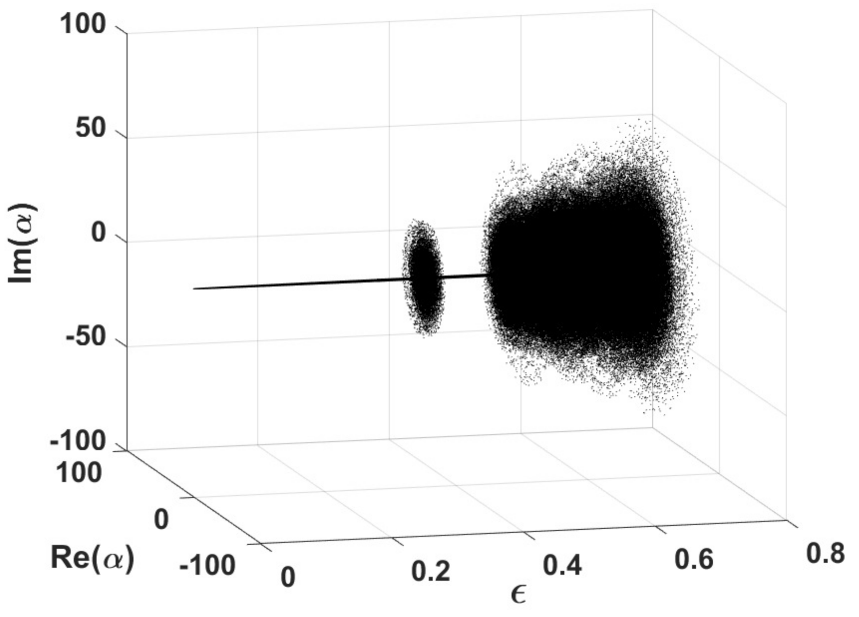
As already mentioned, the classical counterpart of our system exhibits both regular and chaotic behavior for various values of the strength of excitation. To find the borders between the regions of regular and chaotic dynamics, we shall plot a bifurcation diagram (see Figure 1). In this diagram, we present the values of the real and imaginary parts of the complex parameter $\alpha$, which is the classical counterpart of the annihilation operator $\widehat{a}$, and ${\left|\alpha \right|}^2$ is the energy of our system’s classical counterpart. To prepare such a diagram, we use the method described in [44]. With the accordance of this method, we find the equation of motion for the annihilation operator for the time between the subsequent external pulses. Next, we include the influence of the external pulse, and finally, we replace all operators $\widehat{a}$ and ${\widehat{a}}^{†}$, appearing in the solution, by the complex numbers $\alpha$ and ${\alpha }^{\ast }$, respectively. Analysis of the bifurcation diagram shows that the first regular motion region extends for approx $0\le ϵ\lesssim 0.344$. Next, we observe the first, not so broad, chaotic belt as $0.344\lesssim ϵ\lesssim 0.356$, which is followed by a regular window $0.356\lesssim ϵ\lesssim 0.47$. Finally, we observe the deep chaos region for $ϵ\gtrsim 0.47$.

3. Leggett–Garg Inequalities

To analyze nonclassical temporal correlations, we will use the LGI. Assuming an experiment in which two measurements are made at three different times $t_1<t_2<t_3$, we can obtain the simplest form of such inequality. Additionally, the measured observable should be dichotomous, i.e., it has two eigenvalues $Q=\pm 1$. In such a case, the LGI takes the following form:

$$-3\le C_{21}+C_{32}+C_{31}\le 1.$$

(6)

In general, when n measurements ($n>2$) are performed, the LGI can be written as [15,16,56]:

$$\begin{array}{ccc}\hfill -n\le & K_n& \le n-2\mathrm{for}\mathrm{odd}n\ge 3\hfill \\ \hfill -(n-1)\le & K_n& \le n-2\mathrm{for}\mathrm{even}n\ge 4\hfill \end{array}$$

(7)

where $K_n$ is the n-th order correlator defined by the following equation

$$K_n=C_{21}+C_{32}+\dots +C_{n,n-1}-C_{n,1}$$

(8)

and $C_{ij}$ are the correlation functions defined with an application of the joint probability

$$C_{ij}=\sum _{q_j{q}_i}{q}_j{q}_{i}p\left(q_i,t_i;q_j,t_j\right).$$

(9)

The quantity $p\left(q_i,t_i;q_j,t_j\right)$ appearing in (9) is a probability of obtaining the results $q_i$ from measurements performed at the moment of time $t_i$, and the results $q_j$ at the time $t_j$. Such probability can be expressed by [16,57]:

$$p\left(q_i,t_i;q_j,t_j\right)=Tr\left(P_{q_j}{U}_{t_j;t_i}{P}_{q_i}{U}_{t_i;0}\rho (t=0)U_{t_i;0}^{†}{P}_{q_i}{U}_{t_j;t_i}^{†}\right),$$

(10)

where $\rho (t=0)$ is the density matrix describing the system for the initial time $t=0$. The operator $U_{t_j;t_i}$ which appears in Equation (10) is an operator of the evolution between the moments of time $t_j$ and $t_i$ (it corresponds to the time interval $T=t_j-t_i$). For the system analyzed here, the evolution operator is defined by Equations (2)–(4). For the situation discussed here, we will perform measurements just after each pulse.

The measured observable Q is described by the equation:

$$Q=q_{+}{P}_{+}+q_{-}{P}_{-}(q_{\pm }=\pm 1)$$

(11)

where $P_{+}$ and $P_{-}$ are projection operators

$$\begin{array}{ccc}\hfill P_{+}& =& |\mathsf{\Psi }\left(\theta ,\varphi \right)\rangle \langle \mathsf{\Psi }\left(\theta ,\varphi \right)|,\hfill \\ \hfill P_{-}& =& I-P_{+}.\hfill \end{array}$$

(12)

Additionally, in further consideration, we assume that the wave function describing the system is projected onto the vector defined on a Bloch sphere

$$\mathsf{\Psi }\left(\theta ,\varphi \right)={cos}^2\left(\theta /2\right)|0\rangle +e^{i\varphi }{sin}^2\left(\theta /2\right)|1\rangle .$$

(13)

It should be also noted that for projective measurements, the maximal value of the correlator $K_n$ which can be reached is $ncos\left(\pi /n\right)$ [16].

4. Leggett–Garg Inequalities for an Arbitrarily Assumed Time Interval between Measurements

In this section, we concentrate on the dynamics of a quantum nonlinear oscillator characterized by the Kerr-type third-order nonlinearity. We assume that at the initial time $t=0$, the system was the vacuum state $|0\rangle$. Next, the oscillator undergoes excitation in the form of a train of coherent external pulses. Finally, for the moments of time corresponding to each pulse, we perform subsequent measurements—projections on the specific Bloch vectors (the measurements are performed just after each pulse). Those measurements are performed one by one over a period of time $\tau =t_j-t_i=T$. Such measurements allow finding the correlators defined in (8), giving information on whether the appropriate LGIs are violated. The violation of those inequalities implies the existence of nonclassical temporal correlations. Our purpose is to show the relation between the appearance of violations of LGI and the character of the discussed system’s dynamics. We are interested in any difference in the character of the correlators’ evolution appearing when we change the parameters that “switch” the system from the regular to quantum chaotic dynamics. Such differences could be applied as a novel witness of the quantum chaotic dynamics.

In Figure 2, we show the values of the correlators $K_3$–$K_6$ found by taking measurements in a short-time evolution range. This means that the subsequent projections on the Bloch vector are performed in short series, just after two, three, four, or five subsequent excitations. From the results presented in Figure 2, one can see that LGI are violated only for some limited range of Bloch vectors. The width of this range depends strongly on the strength of the external excitations. For the weak excitation case, very narrow windows on $\theta$ angles around 0 and $\pi$ values result in violating inequalities of all analyzed orders for various values of $\varphi$. The degree of violation increases with the order of the correlator (therefore, with the number of performed measurements).

Increasing the excitation’s strength, the range of $\theta$ values for which the LGI are violated initially increases (which is seen in Figure 2a–c, and for larger values of $ϵ$ are present only for $\theta$ close to 0 and $2\pi$ for $K_3$. For higher-order correlators, it is true when we discuss the regions of the parameters for which the quantum oscillator evolves regularly—Figure 2d,e,g,h,j,k. When the excitation strengths are large enough to cause the chaotic evolution of the oscillator, the LGI is no longer violated if we perform more than two subsequent measurements—Figure 2f,i,l.

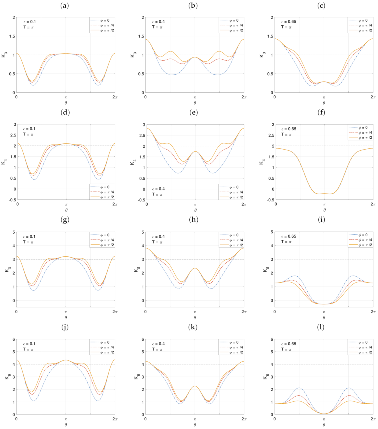
We can consider the values of correlators for the specific choice of the state $\theta =\varphi =0$ to which the projection is performed, as the optimal choice of the state to show the maximum violation of LGI for various values of excitation strength $ϵ$. It is presented in Figure 3, and it is evident that higher-order correlators, like $K_6$, can be used for distinguishing between regular and not regular dynamics of the quantum system. When the classical kicked nonlinear oscillator is in a region of chaotic evolution, its quantum counterpart evolves between a large number of quantum states. It was already shown [44] that for higher excitation strengths, the mean number of photons present in the system significantly increased when compared to oscillations between 0 and 1 photon states in regular dynamics obtained for smaller values of $ϵ$. In [44], it is also shown that such an increase and change in the type of system’s dynamics can be observed after several number of external pulses. Therefore, it seems to be clear that when correlators are defined in such a way that the projective measurement is made after subsequent pulses, the higher range of correlators, the larger number of photons in the system, and any changes in dynamics can be seen better.

5. Leggett–Garg Inequalities and Long-Time Measurements

When examining the inequalities of temporal correlations by using them for differentiating between the regular and chaotic evolution of the quantum system, it will be useful to find the optimal length of time between subsequent measurements for which any differences are visible.

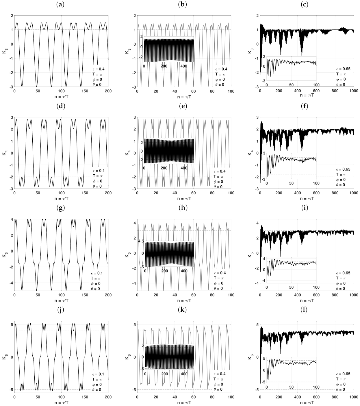
Therefore, in Figure 4, we show the values of correlators up to the 6-th order with respect to the time lengths $\tau$ between performed measurements. These lengths are expressed as a multiple of the unitary evolution time T. Therefore, the longer the time $\tau$, the larger number of external excitations of the oscillator before the measurement occurs. In such a way, via appropriate correlators $K_3-K_6$ defined by Equation (8), we are able to analyze the quantum system’s state after longer times of evolution than in the preceding chapter. It may be of special use when the quantum system does not exhibit regular oscillations, and it starts to evolve chaotically. When studying the dynamics in longer time, if the system does not follow regular oscillations between specific quantum states, it should be seen in the changes of correlators values and consequently in the inequality violation.

We can easily see (Figure 4a,b,d,e,g,h,j,k) the periodic behavior of correlators with the increase of $\tau$ in regions in which the system’s dynamic is regular and quantum oscillator evolves among few quantum number states.

However, when the excitation’s strength $ϵ$ increases to the values for which the classical counterpart of the analyzed system starts to evolve chaotically, such an increase in time length $\tau$ leads to a situation in which LG inequalities are no longer violated for the majority of the analyzed number of excitations n. In that sense, the system loses its quantumness related to time correlations. Occasional increases of the correlators values, sufficient to violate the appropriate LG inequality, come from the fact that for a large number of excitations between subsequent projective measurements, the chaotically evolving oscillator may probably be found accidentally in a quantum state corresponding to the one chosen in (12). The majority of the obtained values of correlators are below their specific border values $ncos\left(\pi /n\right)$ [16], indicating that the evolution of the oscillators is not regular anymore. Such evolution of the described quantum nonlinear oscillator in that sense reflects the adequate evolution and type of dynamics of its classical counterpart and using high-order correlators may be a good choice for distinguishing between various types of dynamics.

When analyzing how the values of appropriate correlators change with increasing time between measurements, we can see that smaller values of $\tau$ result in the violation of inequalities expressed by correlators $K_3$–$K_6$. However, when the time between projective measurements allows for much larger, about several dozen, the number of excitations (see Figure 4c,f,i,l), the LG inequalities are no longer violated.

We can also conclude that the larger the number of pulses and the oscillator evolves longer, not regular oscillations are more easily revealed. When we compare Figure 4c,f,i,l, we can see that the correlator $K_6$ for example, indicates not violating Leggett–Garg inequality after a smaller number of pulses than correlator $K_3$ for the same values of parameters describing the oscillator. This is most likely related to the fact that the method of analyzing the behavior of a system is more sensitive when we apply a higher-order correlator. The use of higher-order correlators allows taking into account a longer part of a time series in the analysis. This is important in the case of a chaotic system where quantum correlations disappear over time and the hold of the correlation for a long time is not possible. Thus, the higher-order correlator is more sensitive to correlation decay.

Such behavior would potentially allow for choosing appropriate $\tau$ values for which one could distinguish between regular and chaotic evolution by correlator’s transition between violating and not violating Leggett–Garg inequalities.

6. Time Evolution in Leggett–Garg Inequalities

The next question which arises is whether the inequalities are violated when analyzing the system constantly evolving in time. Therefore, in Equation (10), instead of the initial system’s state $\rho (t=0)$, the adequate state of the oscillator after n-th excitation is used $\rho (t=nT)$

$$p\left(q_i,t_i;q_j,t_j\right)=Tr\left(P_{q_j}{U}_{t_j;t_i}{P}_{q_i}{U}_{t_i;t=nT}\rho (t=nT)U_{t_i;t=nT}^{†}{P}_{q_i}{U}_{t_j;t_i}^{†}\right).$$

(14)

In such a way, in calculating appropriate correlators, we refer their values to the specific state of the system, which is constantly excited by ultrashort coherent pulses. Time between subsequent measurements stays constant and for our consideration is maintained and equal to $\pi$:

$$\tau =t_2-t_1=t_3-t_2=\pi$$

(15)

The same value takes the time of free evolution between external pulses. Therefore, the nonlinear oscillator evolves in time and is subjected to n excitations while we probe the system and perform projective measurements (find values of correlators) after various time lengths expressed by multiples of T.

In the same manner as it was done in the previous chapters, the main objective is to identify any differences between correlators values, and consequently determine whether LG inequalities are violated or not, in two cases: for an oscillator which evolves regularly between quantum states, and an oscillator which can be treated as a chaotic one.

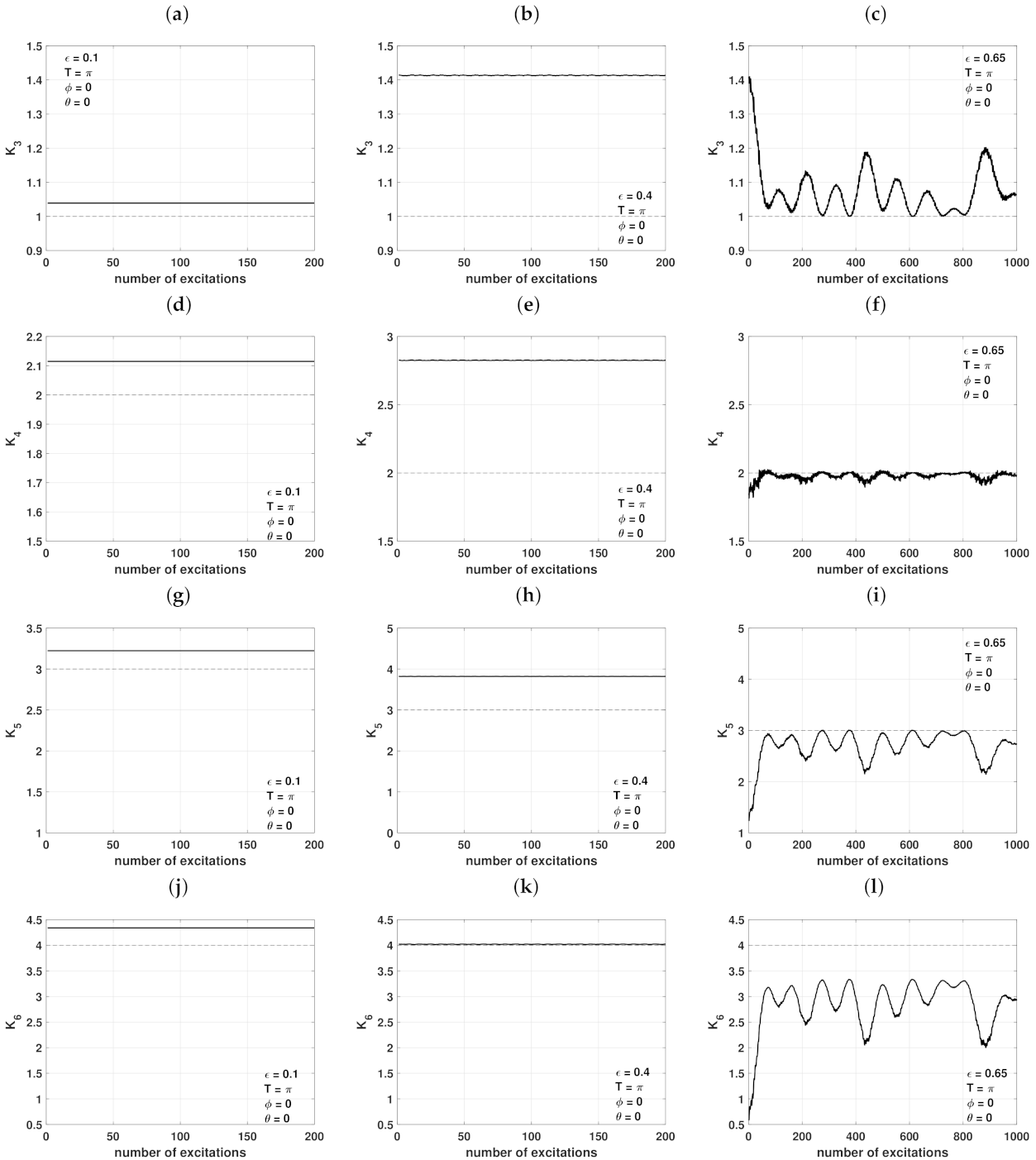
As an example, in Figure 5, we show the time evolution of correlators $K_3$ – $K_6$ for the state $\mathsf{\Psi }\left(\theta =0,\varphi =0\right)$, which is the optimal choice when maximizing the correlators values for the nonlinear oscillator.

We can clearly see the values of correlators of all analyzed orders when the oscillator is weakly excited and evolves regularly among the limited number of quantum states indicate the violating of Leggett–Garg inequalities throughout the whole evolution time—Figure 5a,b,d,e,g,h,j,k. When the excitation strength $ϵ$ exceeds 0.5, which is the value for which the classical counterpart of the oscillator is within the chaotic region, the time evolution of correlators values changes its character—Figure 5c,f,i,l. The lowest level correlator $K_3$ initially decreases its value, and after that some, oscillations close to the border value $K_3=1$ are visible. Nevertheless, during the whole analyzed time, Leggett–Garg inequality is violated, indicating the existence of quantum temporal correlations in the system.

Correlators of higher values $K_4$, $K_5$, and $K_6$, which give information about correlations when three, four, or five subsequent projective measurements are performed, for large excitation values, drop below the border values indicating that Leggett–Garg inequalities are no longer violated. All correlators indicate a type of perturbed oscillatory evolution in that region and only fourth-order time correlator $K_4$ during these oscillations is able to slightly exceed the border line ($K_4=2$). This behavior is maintained throughout the whole evolution time. Therefore, analyses of these correlators seem promising when distinguishing between different types of dynamics of the analyzed system. For the optimal choice of the state $\mathsf{\Psi }\left(\theta ,\varphi \right)$, the transition between violating and not violating the higher-order correlators suggests a change in the type of evolution of the quantum system. Moreover, we come to the conclusion that, for that purpose, the better solution would be to use higher-order correlators (as $K_5$ for example). Increasing the number of projective measurements during the evolution of a not regularly evolving quantum system, one may obtain a better parameter to distinguish between the types of system’s dynamics.

Moreover, it comes to the conclusion that, for that purpose, the better solution would be to use higher-order correlators (as $K_5$ for example). As mentioned earlier, the use of higher-order correlators allows covering a longer part of a time series in the analysis. Then, the analysis method based on higher-order correlators is more sensitive to the disappearance of the correlation between the elements of the time series. It is particularly important in the case of the chaotic evolution of a system, where quantum correlations disappear over time. Therefore, increasing the number of projective measurements during the evolution of not regularly evolving quantum systems, one may obtain a better parameter to distinguish between the types of system’s dynamics.

7. Conclusions

We propose the use of inequalities based on temporal correlations between the states of a system which is exposed to several projective measurements for distinguishing between the regular and chaotic evolution of a given quantum system. We have decided to analyze a simple nonlinear oscillator which is externally driven by a series of ultrashort pulses. That specific system was described and reported as an example of both a regularly and chaotically evolving one, depending on the strength of the excitations applied to the system. A thorough analysis has already been performed when assuming classical and quantum descriptions of that model.

In this paper, we focus on the temporal correlations between the outcomes of the measurements made on that quantum system. The measurements that are taken are the projections on the vector taken from the Bloch sphere $\mathsf{\Psi }\left(\theta ,\varphi \right)={cos}^2\left(\theta /2\right)|0\rangle +e^{i\varphi }{sin}^2\left(\theta /2\right)|1\rangle .$ In our considerations, we analyze Leggett–Garg inequalities based on correlators of various orders $K_3$, $K_4$, $K_5$, and $K_6$ which give us information about temporal correlations within the system when making 2, 3, 4 or 5 subsequent measurements. Our purpose was to find whether a violation of Leggett–Garg inequality will reflect the type of dynamics the quantum system follows. Therefore, we have compared the adequate values of correlators (8) in various ranges of parameters identifying our system. We have obtained the optimal values of angles $\theta$ and $\varphi$ for maximal Leggett–Garg inequality violation and for that specific choice showed the differences in correlators values when the oscillator evolves regularly between a few quantum states and can be considered as a chaotic one. We have considered the behavior of the correlators when the projections were made just after the initial system’s excitation. Additionally, we analyzed the same parameters when assuming that the time between subsequent measurements is longer and defined as a multiple of the excitation.

In all of these cases, we have found that the transition between a violation and no violation of the Leggett–Garg inequality can be associated with regular and not regular dynamics, when the oscillator is excited several times before the measurements are made. This does not influence the result in the regular dynamics region but is important when the system evolution is no longer regular. The longer the evolution of the quantum system with nonregular dynamics, the less likely one is to observe the violation of LG inequalities. Additionally, we have found that for such cases, the types of dynamics are the higher-order correlators, which are more fragile. This is associated with a larger number of measurements performed on the system at various moments during its evolution. Whenever our quantum system is evolving in a nonregular way among a large number of quantum states, such multiple “probing” reveals the lack of correlation between the measurements’ outcomes in the time domain.

Then, the non-classicality associated with temporal correlations is destroyed. For that reason, it is also better to use more than 3 correlators’ orders, which ensure that the number of measurements increases and consequently the time of the whole evolution is significantly longer.

The same happens when taking into consideration the time evolution of the whole system and for each of the measurements take the state of the system after time t—the state of the oscillator after n-th excitation (14). Once more, when the quantum system is far from regular oscillations, it is reflected in correlators (of higher than 3 order) values.

Therefore, we believe that temporal correlation analysis can also be adapted as a tool in the field of regular and chaotic evolution of quantum systems. It would be valuable if it was possible to carry out an appropriate experiment confirming the possibility of analyzing LGI inequality violation in the context of regular or chaotic evolution of the quantum system under study. Potentially, some of the attempts may be associated with systems such as optical lattices [58]. It would also allow for the extension of the method in the experimental aspect, using the already described noninvasive measurements. For instance, in the system of cold atoms in an optical lattice, the absence of atoms at a chosen lattice site without affecting them was probed [20].

References

- Cubitt, T.S.; Verstraete, F.; Cirac, J.I. Entanglement flow in multipartite systems. Phys. Rev. A 2005, 71, 052308. [Google Scholar] [CrossRef] [Green Version]
- López, C.E.; Romero, G.; Lastra, F.; Solano, E.; Retamal, J.C. Sudden Birth versus Sudden Death of Entanglement in Multipartite Systems. Phys. Rev. Lett. 2008, 101, 080503. [Google Scholar] [CrossRef] [PubMed] [Green Version]
- Kurpas, M.; Dajka, J.; Zipper, E. Entanglement of qubits via a nonlinear resonator. J. Phys. Condens. Matter 2009, 21, 235602. [Google Scholar] [CrossRef] [PubMed]
- Mohamed, A.; Eleuch, H. Non-classical effects in cavity QED containing a nonlinear optical medium and a quantum well: Entanglement and non-Gaussanity. Eur. Phys. J. D 2015, 69, 191. [Google Scholar] [CrossRef]
- Nowakowski, M. Quantum entanglement in time. AIP Conf. Proc. 2017, 1841, 020007. [Google Scholar] [CrossRef] [Green Version]
- Schrödinger, E. Discussion of Probability Relations between Separated Systems. Math. Proc. Camb. Philos. Soc. 1935, 31, 555–563. [Google Scholar] [CrossRef]
- Chowdhury, P.; Pramanik, T.; Majumdar, A.S.; Agarwal, G.S. Einstein-Podolsky-Rosen steering using quantum correlations in non-Gaussian entangled states. Phys. Rev. A 2014, 89, 012104. [Google Scholar] [CrossRef] [Green Version]
- He, Q.; Rosales-Zárate, L.; Adesso, G.; Reid, M.D. Secure Continuous Variable Teleportation and Einstein-Podolsky-Rosen Steering. Phys. Rev. Lett. 2015, 115, 180502. [Google Scholar] [CrossRef] [Green Version]
- Kocsis, S.; Hall, M.J.W.; Bennet, A.J.; Saunders, D.J.; Pryde, G.J. Experimental measurement-device-independent verification of quantum steering. Nat. Commun. 2015, 6, 5886. [Google Scholar] [CrossRef]
- Jebaratnam, C.; Das, D.; Roy, A.; Mukherjee, A.; Bhattacharya, S.S.; Bhattacharya, B.; Riccardi, A.; Sarkar, D. Tripartite-entanglement detection through tripartite quantum steering in one-sided and two-sided device-independent scenarios. Phys. Rev. A 2018, 98, 022101. [Google Scholar] [CrossRef] [Green Version]
- Bell, J.S. On the Einstein Podolsky Rosen paradox. Phys. Phys. Fiz. 1964, 1, 195–200. [Google Scholar] [CrossRef] [Green Version]
- Jones, S.J.; Wiseman, H.M.; Doherty, A.C. Entanglement, Einstein-Podolsky-Rosen correlations, Bell nonlocality, and steering. Phys. Rev. A 2007, 76, 052116. [Google Scholar] [CrossRef] [Green Version]
- Brunner, N.; Cavalcanti, D.; Pironio, S.; Scarani, V.; Wehner, S. Bell nonlocality. Rev. Mod. Phys. 2014, 86, 419–478. [Google Scholar] [CrossRef] [Green Version]
- Quintino, M.T.; Vértesi, T.; Cavalcanti, D.; Augusiak, R.; Demianowicz, M.; Acín, A.; Brunner, N. Inequivalence of entanglement, steering, and Bell nonlocality for general measurements. Phys. Rev. A 2015, 92, 032107. [Google Scholar] [CrossRef] [Green Version]
- Leggett, A.J.; Garg, A. Quantum mechanics versus macroscopic realism: Is the flux there when nobody looks? Phys. Rev. Lett. 1985, 54, 857–860. [Google Scholar] [CrossRef] [PubMed] [Green Version]
- Emary, C.; Lambert, N.; Nori, F. Leggett–Garg inequalities. Rep. Prog. Phys. 2013, 77, 016001. [Google Scholar] [CrossRef]
- Morikoshi, F. Information-theoretic temporal Bell inequality and quantum computation. Phys. Rev. A 2006, 73, 052308. [Google Scholar] [CrossRef] [Green Version]
- Palacios-Laloy, A.; Mallet, F.; Nguyen, F.; Bertet, P.; Vion, D.; Esteve, D.; Korotkov, A.N. Experimental violation of a Bell’s inequality in time with weak measurement. Nat. Phys. 2010, 6, 442–447. [Google Scholar] [CrossRef] [Green Version]
- Knee, G.C.; Simmons, S.; Gauger, E.M.; Morton, J.J.; Riemann, H.; Abrosimov, N.V.; Becker, P.; Pohl, H.J.; Itoh, K.M.; Thewalt, M.L.; et al. Violation of a Leggett–Garg inequality with ideal non-invasive measurements. Nat. Commun. 2012, 3, 606. [Google Scholar] [CrossRef] [Green Version]
- Robens, C.; Alt, W.; Meschede, D.; Emary, C.; Alberti, A. Ideal Negative Measurements in Quantum Walks Disprove Theories Based on Classical Trajectories. Phys. Rev. X 2015, 5, 011003. [Google Scholar] [CrossRef] [Green Version]
- Athalye, V.; Roy, S.S.; Mahesh, T.S. Investigation of the Leggett-Garg Inequality for Precessing Nuclear Spins. Phys. Rev. Lett. 2011, 107, 130402. [Google Scholar] [CrossRef] [PubMed]
- Waldherr, G.; Neumann, P.; Huelga, S.F.; Jelezko, F.; Wrachtrup, J. Violation of a Temporal Bell Inequality for Single Spins in a Diamond Defect Center. Phys. Rev. Lett. 2011, 107, 090401. [Google Scholar] [CrossRef] [PubMed] [Green Version]
- George, R.E.; Robledo, L.M.; Maroney, O.J.E.; Blok, M.S.; Bernien, H.; Markham, M.L.; Twitchen, D.J.; Morton, J.J.L.; Briggs, G.A.D.; Hanson, R. Opening up three quantum boxes causes classically undetectable wavefunction collapse. Proc. Natl. Acad. Sci. USA 2013, 110, 3777–3781. [Google Scholar] [CrossRef] [PubMed] [Green Version]
- Souza, A.M.; Oliveira, I.S.; Sarthour, R.S. A scattering quantum circuit for measuring Bell’s time inequality: a nuclear magnetic resonance demonstration using maximally mixed states. New J. Phys. 2011, 13, 053023. [Google Scholar] [CrossRef]
- Katiyar, H.; Shukla, A.; Rao, K.R.K.; Mahesh, T.S. Violation of entropic Leggett-Garg inequality in nuclear spins. Phys. Rev. A 2013, 87, 052102. [Google Scholar] [CrossRef] [Green Version]
- Goggin, M.E.; Almeida, M.P.; Barbieri, M.; Lanyon, B.P.; O’Brien, J.L.; White, A.G.; Pryde, G.J. Violation of the Leggett–Garg inequality with weak measurements of photons. Proc. Natl. Acad. Sci. USA 2011, 108, 1256–1261. [Google Scholar] [CrossRef] [Green Version]
- Xu, J.S.; Li, C.F.; Zou, X.B.; Guo, G.C. Experimental violation of the Leggett-Garg inequality under decoherence. Sci. Rep. 2011, 1, 101. [Google Scholar] [CrossRef] [Green Version]
- Dressel, J.; Broadbent, C.J.; Howell, J.C.; Jordan, A.N. Experimental Violation of Two-Party Leggett-Garg Inequalities with Semiweak Measurements. Phys. Rev. Lett. 2011, 106, 040402. [Google Scholar] [CrossRef] [Green Version]
- Suzuki, Y.; Iinuma, M.; Hofmann, H.F. Violation of Leggett–Garg inequalities in quantum measurements with variable resolution and back-action. New J. Phys. 2012, 14, 103022. [Google Scholar] [CrossRef]
- Schuster, H.G.; Just, W. Deterministic Chaos—An Introduction; Wiley-VCH Verlag: Weinheim, Germany, 2005. [Google Scholar]
- Gharibyan, H.; Hanada, M.; Swingle, B.; Tezuka, M. Characterization of quantum chaos by two-point correlation functions. Phys. Rev. E 2020, 102, 022213. [Google Scholar] [CrossRef]
- De la Cruz, J.; Lerma-Hernández, S.; Hirsch, J.G. Quantum chaos in a system with high degree of symmetries. Phys. Rev. E 2020, 102, 032208. [Google Scholar] [CrossRef] [PubMed]
- Miller, P.A.; Sarkar, S. Signatures of chaos in the entanglement of two coupled quantum kicked tops. Phys. Rev. E 1999, 60, 1542–1550. [Google Scholar] [CrossRef] [PubMed]
- Tanaka, A.; Fujisaki, H.; Miyadera, T. Saturation of the production of quantum entanglement between weakly coupled mapping systems in a strongly chaotic region. Phys. Rev. E 2002, 66, 045201. [Google Scholar] [CrossRef] [Green Version]
- Wang, X.; Ghose, S.; Sanders, B.C.; Hu, B. Entanglement as a signature of quantum chaos. Phys. Rev. E 2004, 70, 016217. [Google Scholar] [CrossRef] [PubMed] [Green Version]
- Trail, C.M.; Madhok, V.; Deutsch, I.H. Entanglement and the generation of random states in the quantum chaotic dynamics of kicked coupled tops. Phys. Rev. E 2008, 78, 046211. [Google Scholar] [CrossRef] [Green Version]
- Dajka, J.; Łobejko, M.; Łuczka, J. Leggett–Garg inequalities for a quantum top affected by classical noise. Quantum Inf. Process. 2016, 15, 4911–4925. [Google Scholar] [CrossRef] [Green Version]
- Ban, M. Leggett-Garg Inequality and Quantumness Under the Influence of Random Telegraph Noise. Int. J. Theor. Phys. 2019, 58, 2893–2909. [Google Scholar] [CrossRef]
- Leoński, W.; Tanaś, R. Possibility of producing the one-photon state in a kicked cavity with a nonlinear Kerr medium. Phys. Rev. A 1994, 49, R20–R23. [Google Scholar] [CrossRef]
- Leoński, W.; Dyrting, S.; Tanaś, R. One-Photon State Generation in a Kicked Cavity with Nonlinear Kerr Medium. In Coherence and Quantum Optics VII; Eberly, J.H., Mandel, L., Wolf, E., Eds.; Springer: Boston, MA, USA, 1996; pp. 425–426. [Google Scholar] [CrossRef]
- Milburn, G.J.; Holmes, C.A. Dissipative Quantum and Classical Liouville Mechanics of the Anharmonic Oscillator. Phys. Rev. Lett. 1986, 56, 2237. [Google Scholar] [CrossRef]
- Szlachetka, P.; Grygiel, K.; Bajer, J. Chaos and order in a kicked anharmonic oscillator: Classical and quantum analysis. Phys. Rev. E 1993, 48, 101–108. [Google Scholar] [CrossRef]
- Kowalewska-Kudłaszyk, A.; Kalaga, J.K.; Leoński, W. Wigner-function nonclassicality as indicator of quantum chaos. Phys. Rev. E 2008, 78, 066219. [Google Scholar] [CrossRef] [PubMed] [Green Version]
- Leoński, W. Quantum and classical dynamics for a pulsed nonlinear oscillator. Phys. A 1996, 233, 365–378. [Google Scholar] [CrossRef]
- Bose, S.; Jacobs, K.; Knight, P.L. Preparation of nonclassical states in cavities with a moving mirror. Phys. Rev. A 1997, 56, 4175–4186. [Google Scholar] [CrossRef] [Green Version]
- Wang, H.; Gu, X.; Liu, Y.X.; Miranowicz, A.; Nori, F. Tunable photon blockade in a hybrid system consisting of an optomechanical device coupled to a two-level system. Phys. Rev. A 2015, 92, 033806. [Google Scholar] [CrossRef] [Green Version]
- Wallentowitz, S.; Vogel, W. Quantum-mechanical counterpart of nonlinear optics. Phys. Rev. A 1997, 55, 4438–4442. [Google Scholar] [CrossRef] [Green Version]
- Jacobs, K. Engineering Quantum States of a Nanoresonator via a Simple Auxiliary System. Phys. Rev. Lett. 2007, 99, 117203. [Google Scholar] [CrossRef] [Green Version]
- Greentree, A.D.; Tahan, C.; Cole, J.H.; Hollenberg, L.C.L. Quantum phase transitions of light. Nat. Phys. 2006, 2, 856–861. [Google Scholar] [CrossRef] [Green Version]
- Kühner, T.D.; Monien, H. Phases of the one-dimensional Bose-Hubbard model. Phys. Rev. B 1998, 58, R14741–R14744. [Google Scholar] [CrossRef] [Green Version]
- Jaksch, D.; Bruder, C.; Cirac, J.I.; Gardiner, C.W.; Zoller, P. Cold Bosonic Atoms in Optical Lattices. Phys. Rev. Lett. 1998, 81, 3108–3111. [Google Scholar] [CrossRef]
- Peřinová, V.; Lukš, A.; Křapelka, J. Dynamics of nonclassical properties of two- and four-mode Bose-Einstein condensates. J. Phys. B At. Mol. Opt. Phys. 2013, 46, 195301. [Google Scholar] [CrossRef]
- Birnbaum, K.M.; Boca, A.; Miller, R.; Boozer, A.D.; Northup, T.E.; Kimble, H.J. Photon blockade in an optical cavity with one trapped atom. Nature 2005, 436, 87. [Google Scholar] [CrossRef] [PubMed] [Green Version]
- Lang, C.; Bozyigit, D.; Eichler, C.; Steffen, L.; Fink, J.M.; Abdumalikov, A.A.; Baur, M.; Filipp, S.; da Silva, M.P.; Blais, A.; et al. Observation of Resonant Photon Blockade at Microwave Frequencies Using Correlation Function Measurements. Phys. Rev. Lett. 2011, 106, 243601. [Google Scholar] [CrossRef] [PubMed] [Green Version]
- Miranowicz, A.; Bajer, J.; Paprzycka, M.; Liu, Y.; Zagoskin, A.M.; Nori, F. State-dependent photon blockade via quantum-reservoir engineering. Phys. Rev. A 2014, 90, 033831. [Google Scholar] [CrossRef] [Green Version]
- Leggett, A.J. Testing the limits of quantum mechanics: motivation, state of play, prospects. J. Phys. Condens. Matter 2002, 14, R415–R451. [Google Scholar] [CrossRef] [Green Version]
- Budroni, C.; Emary, C. Temporal Quantum Correlations and Leggett-Garg Inequalities in Multilevel Systems. Phys. Rev. Lett. 2014, 113, 050401. [Google Scholar] [CrossRef] [PubMed] [Green Version]
- Prants, S.V. Hamiltonian Chaos with a Cold Atom in an Optical Lattice. In Hamiltonian Chaos Beyond the KAM Theory: Dedicated to George M. Zaslavsky (1935–2008); Luo, A.C.J., Afraimovich, V., Eds.; Springer: Berlin/Heidelberg, Germany, 2010; pp. 193–223. [Google Scholar] [CrossRef]
Figure 1.
Bifurcation diagram for the real and imaginary parts of as a function of the strength of external excitation for the nonlinearity parameter and the time between subsequent pulses .
Figure 2.
At (a–c) correlator; at (d–f) correlator; at (g–i) correlator and at (j–l) correlator for a single nonlinear oscillator exposed to a series of ultra-short excitations of various strengths . Time between pulses ; times between projective measurements: . Initial state of the system is and state . The horizontal dashed lines represent the border between values of excluded and not excluded by the Leggett–Garg inequality.
Figure 3.
– correlators versus for a single nonlinear oscillator exposed to a series of ultra-short excitations. Time between pulses ; times between projective measurements: . Initial state of the system is and state . The horizontal lines represent the border between values of excluded and not excluded by the Leggett–Garg inequality.
Figure 4.
At (a–c) correlator; at (d–f) correlator; at (g–i) correlator and at (j–l) correlator for a single nonlinear oscillator exposed to a series of ultra-short excitations of various strengths . Time between pulses ; times between projective measurements: . Initial state of the system is and state . The horizontal dashed lines represent the border between values of excluded and no excluded by the Leggett–Garg inequality.
Figure 5.
At (a–c) correlator; at (d–f) correlator; at (g–i) correlator and at (j–l) correlator for a single nonlinear oscillator exposed to a series of ultra-short excitations of various strengths . Time between pulses ; times between projective measurements: . Initial state for (14) is a state of the oscillator after n-th excitation. State . The horizontal dashed lines represent the border between values of excluded and no excluded by the Leggett–Garg inequality.
Publisher’s Note: MDPI stays neutral with regard to jurisdictional claims in published maps and institutional affiliations. |
© 2021 by the authors. Licensee MDPI, Basel, Switzerland. This article is an open access article distributed under the terms and conditions of the Creative Commons Attribution (CC BY) license (http://creativecommons.org/licenses/by/4.0/).
Share and Cite
MDPI and ACS Style
Kalaga, J.K.; Kowalewska-Kudłaszyk, A.; Nowotarski, M.; Leoński, W. Violation of Leggett–Garg Inequalities in a Kerr-Type Chaotic System. Photonics 2021, 8, 20. https://0-doi-org.brum.beds.ac.uk/10.3390/photonics8010020
AMA Style
Kalaga JK, Kowalewska-Kudłaszyk A, Nowotarski M, Leoński W. Violation of Leggett–Garg Inequalities in a Kerr-Type Chaotic System. Photonics. 2021; 8(1):20. https://0-doi-org.brum.beds.ac.uk/10.3390/photonics8010020
Chicago/Turabian StyleKalaga, Joanna K., Anna Kowalewska-Kudłaszyk, Mateusz Nowotarski, and Wiesław Leoński. 2021. "Violation of Leggett–Garg Inequalities in a Kerr-Type Chaotic System" Photonics 8, no. 1: 20. https://0-doi-org.brum.beds.ac.uk/10.3390/photonics8010020
Note that from the first issue of 2016, this journal uses article numbers instead of page numbers. See further details here.