Target Tracking and Ranging Based on Single Photon Detection

Abstract

In order to achieve non-cooperative target tracking and ranging in conditions of a weak echo signal, this paper presents a real-time acquisition, pointing, tracking (APT), and ranging (APTR) lidar system based on single photon detection. With this system, an active target APT mechanism based on a single photon detector is proposed. The target tracking and ranging strategy and the simulation of target APT are presented. Experiments in the laboratory show that the system has good performance to achieve the acquisition, pointing and ranging of a static target, and track a dynamic target (angular velocity around 3 mrad/s) under the condition of extremely weak echo signals (a dozen photons). Meanwhile, through further theoretical analysis, it can be proven that the mechanism has stronger tracking and detection ability in long distance. It can achieve the active tracking of the target with a lateral velocity of hundreds of meters per second at about one hundred kilometers distance. This means that it has the ability of fast long-distance non-cooperative target tracking and ranging, only by using a single-point single photon detector.

1. Introduction

With the development of science and technology, lidar-based tracking and ranging technology is more widely used in many fields, such as aerospace, automatic driving, etc. [1,2,3,4,5,6,7,8]. It has significant application value for target search, tracking, motion obstacle avoidance, etc. In recent years, to improve the detection capability in conditions of a weak echo signal for hard targets in free-space, single photon detection (SPD) technology was introduced. The SPD can offer the ability to respond to a single photon [5,9,10,11,12]. By using time-correlated single photon counting (TCSPC), the SPD’s sensitivity can be greatly improved, far surpassing classical devices such as linear mode APD or PIN diode, and the needed photon flux is also lower. In this case, the SPD will allow the use of low-power laser sources to detect non-cooperative targets in conditions of a weak echo signal. Currently, most of the research mainly focuses on the rapid detection of weak signals, long-distance high-precision measurement, ranging performance, and imaging [13,14,15,16,17,18,19] based on single photon detection. However, there are few tracking researches based on single photon detection.

To study the tracking technology based on single photon detection, Du et al. [10] provided a new method to simulate the process of tracking the non-cooperative object that moves beyond visual range with a photon-counting laser ranging system. Related algorithms are used to extract and predict the radial trajectory of the target. However, the article does not involve lateral movement detection and has not achieved real tracking. Wu et al. [5] studied the track of moving target by single photon lidar (SPL) in marine aerosol environment. The system realizes the tracking and ranging of the target by combining the imaging system and the single photon ranging system. At present, for moving targets, CCD, CMOS, and other imaging devices are usually used for passive tracking, and, at the same time, coaxial laser ranging is carried out.

Passive detectors such as CCD and CMOS can only work when the target is illuminated, which has great limitations [20]. Four-quadrant detectors and array detectors can simultaneously obtain the orientation and distance information of the target, and can realize active tracking of targets. However, they need cooperative targets and a standard round image spot on the detector to extract the angle information of the target. Moreover, they are affected by the difference in detection units’ parameters, crosstalk between detection units, the echo spot size, and the dead zone [21,22]. When the total energy received by the optical system is certain, the average energy detected on each unit of these detectors is lower than that of the SPD. Moreover, it is difficult to measure direction for non-cooperative targets in conditions of a weak echo signal.

In this paper, we design an APTR lidar system by combining the scanning module with the single photon detection module and achieve distance detection and orientation detection of targets in conditions of a weak echo signal. The scanning module is also used as both the orientation detection module and the servo tracking module, and the system features simple light circuit and convenient adjustment. Moreover, we improve the target detection capability by providing the pulse accumulation method and centroid algorithm in the signal-processing control module. Finally, the system completes the target’s acquisition, pointing tracking, and ranging by selecting an appropriate number of accumulated pulses in conditions of a weak echo signal. The experimental result shows that the target can be captured, pointed, and tracked, and the distance of the target is also displayed in real time. In addition, through further theoretical analysis, it has been proven that the system has stronger tracking and detection ability in long distance by designing a set of practical and feasible system parameters. It can achieve the active tracking of the target with a lateral velocity of hundreds of meters per second at about one hundred kilometers distance only by using a single-point single photon detector. It is potential and meaningful for the fast long-distance non-cooperative target acquisition, tracking, and ranging.

2. Experimental Setup Description

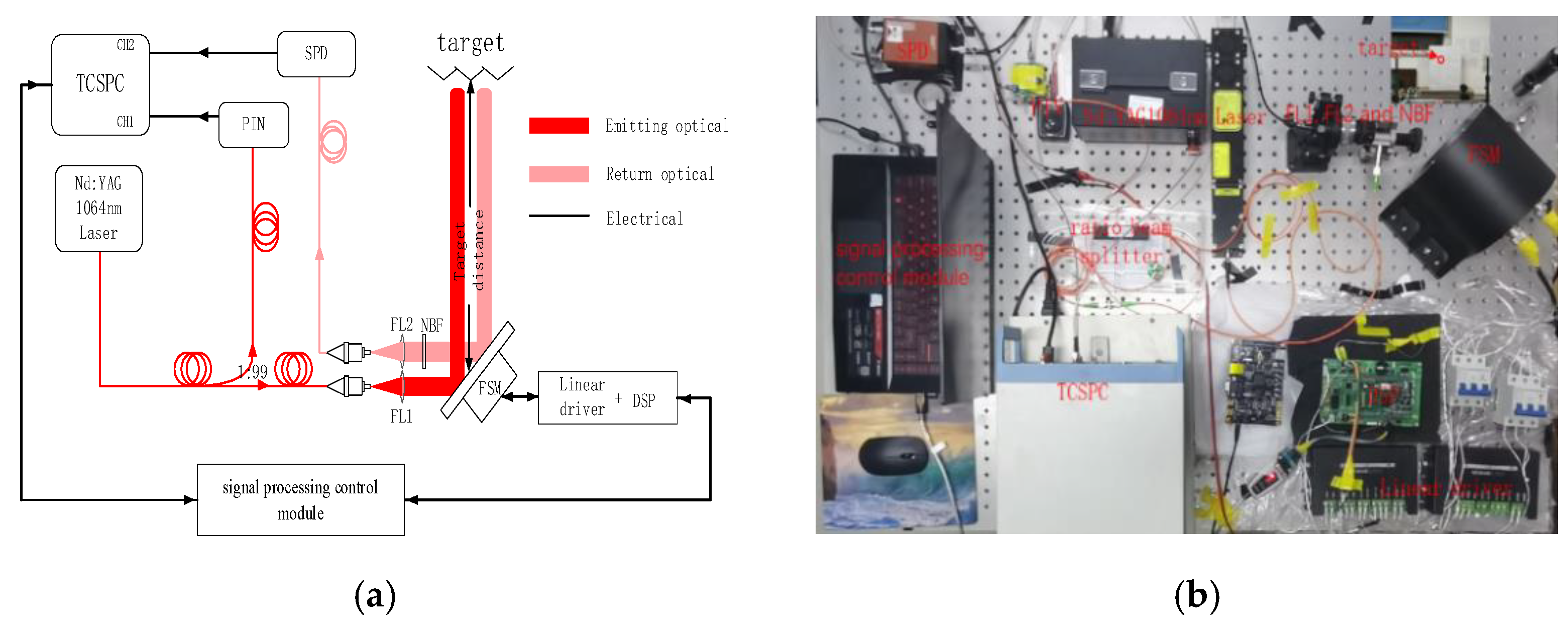
To achieve the APTR of the non-cooperative target based on single photon detection under a weak echo signal, we design the block diagram of APTR system and set up the experimental platform of APTR system. As shown in Figure 1a,b, the laser beam from Nd:YAG (1064 nm) pulsed laser is split into two branches by a ratio beam splitter. The small part of the energy is detected by a PIN, which is used as the synchronous signal, and the other part is transmitted to the target through the optical emitting system (FL1) and fast steering mirror (FSM). The echo signal scattered by the target is coupled into the optical fiber and detected by the SPD through FSM, a narrow bandpass filter (NBF), and an optical receiving system (FL2). The NBF is used to remove most of the background noise from sunlight and other sources. Therefore, the system has the advantages of light circuit and convenient adjustment.

In addition, the signal-processing control module communicates with the single photon detection module (TCSPC, SPD, and PIN) and the scanning module (FSM, linear drive, and DSP). On the one hand, the signal-processing control module controls TCSPC to collect the time and channel information of synchronous signal and echo signal. It also records and decodes the data information. On the other hand, it controls the FSM to scan the target, collects the angle information feedback from the FSM, and decodes the angle information. The pulse accumulation method and the centroid algorithm are used to process the target echo information in the signal processing control module. The signal-processing control module can match the angle information and the target range information to obtain the target’s three-dimensional point clouds and the target centroid position. Finally, the scanning module points to the target centroid and takes the orientation of the target centroid as the scanning center.

3. Single Photon Detection Model and Scanning Model and Target Position

To study APTR of the non-cooperative target based on single photon detection, the paper has the theoretical analysis of the single photon detection model and scanning model. Then the appropriate parameters can be selected to set the system and optimize the collected data. Furthermore, for showing and understanding the process of extracting and tracking the target, we also derive and analyze the three-dimensional coordinates and orientation of the target and the angle coordinates of the scanning center.

3.1. Single Photon Detection Model and Analysis

According to the statistical optics theory, as the echo signal reflected from the rough surface is weak, the number of detected photoelectrons follows Poisson statistics [23,24,25]. The distribution is given as follows:

$$P\left(k\right)=\frac{e^{-{\eta }_{qe}\cdot \left(n_s+n_n\right)}{({\eta }_{qe}\cdot \left(n_s+n_n\right))}^k}{k!},$$

(1)

where $P\left(k\right)$ is the probability that $k$ photoelectrons are detected in a time bin; $n_s$ and $n_n$ are the average number of signal and noise photons in a time bin, respectively; and ${\eta }_{qe}$ is the quantum efficiency of SPD.

The SPD will be triggered when at least one photoelectron (a photon event) occurs in a time bin. Thus, the detection probability ($P_{DS}$) is given by the following:

$$P_{DS}=P_A\left(1-P\left(k=0\right)\right)=P_A(1-e^{\left(-{\eta }_{qe}\cdot \left(n_s+n_n\right)\right)}),$$

(2)

where $P_A=1/\left(1+{\eta }_{qe}·{\phi }_0·t_d\right)$ is the arm probability, and ${\phi }_0$ and $t_d$ are mean noise photon count and dead time, respectively.

When the pulsed laser is shut down, no echo photon signal is collected. In this case, the false-alarm probability ($P_{FAS}$) of a time bin can be obtained by simplifying Equation (2), which is given by the following:

$$P_{FAS}=P_A(1-e^{\left(-{\eta }_{qe}\cdot n_n\right)}),$$

(3)

In fact, a photon event cannot be distinguished from the noise photon events by a single-pulse echo. Therefore, it is necessary to accumulate echo events. If the number of accumulated events exceeds a certain threshold, the target is considered to be found [13,24,26]. An appropriate threshold and pulse accumulation number can effectively reduce the false-alarm probability and improve the detection performance. Assuming that $N$ pulse echoes are accumulated, the detection probability and false-alarm probability of $N$ pulses accumulated in a time bin are as follows:

$$P_D=1-{\sum }_{k^{\prime }=0}^{k_{th}-1}{C}_N^{k^{\prime }}{[P_{DS}]}^{k^{\prime }}{[1-P_{DS}]}^{N-k^{\prime }},$$

(4)

$$P_{FA}=1-{\sum }_{k^{\prime }=0}^{k_{th}-1}{C}_N^{k^{\prime }}{[P_{FAS}]}^{k^{\prime }}{[1-P_{FAS}]}^{N-k^{\prime }},$$

(5)

where $k_{th}$ is the threshold of the recognition target in a time bin, $k^{\prime }$ is the index ranging from 0 to $k_{th}-1$, and $N$ is the number of accumulated pulses. Moreover, $C_N^{k^{\prime }}=\frac{N!}{k^{\prime }!\left(N-k^{\prime }\right)!}$ is the number of combinations of $N$ pulses accumulation taken by $k^{\prime }$ at a time. Here, considering the low light level environment, pile-up effect [27] or dead time effect could be ignored, and $P_A$ is approximate to 1.

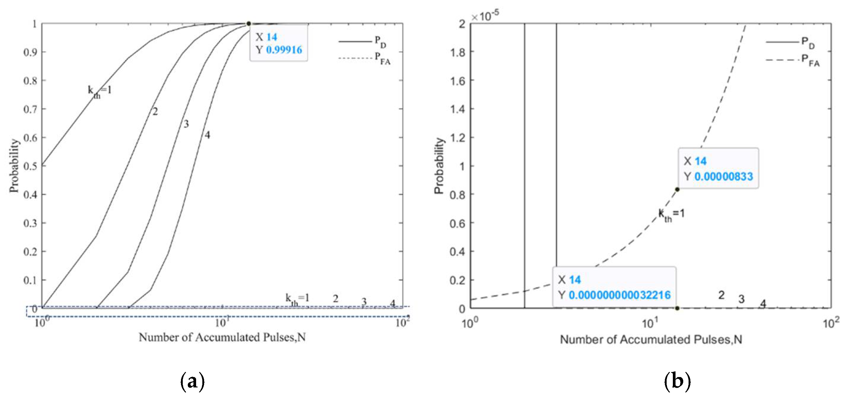
Here, we suppose the laser repetition frequency is 5 kHz, the pulse width is 10 ns, the quantum efficiency (${\eta }_{qe}$) of SPD is 7%, and the time bin is 10 ns, which is consistent with the laser pulse width. The received average number of noise photons ($n_n$) is 8.5 × 10⁻⁶ in a time bin (10 ns) and 0.17 in each cycle (0.2 ms). The received average number of signal photons ($n_s$) is 10. As shown in the Figure 2, the detection probability and false-alarm probability increase with the increase of the number of accumulated pulses. However, when the number of accumulated pulses is fixed, the detection probability and false-alarm probability decrease with the threshold increase, and the false-alarm probability decreases more obviously. Therefore, we can appropriately increase the threshold and the number of accumulated pulses to reduce the false-alarm probability and improve the detection probability.

Assuming the threshold is 1 in a time bin (10 ns), the received average number of noise photons $n_n$ is 8.5 × 10⁻⁶, and the Quantum detection efficiency ${\eta }_{qe}$ is 7%. Figure 3 shows that the target detection probability will increase as the number of echo photons or the number of accumulated pulses increases, when the threshold and the average number of noise photons is fixed. The target false-alarm probability increases with the number of accumulated pulses increase, but the increase rate is low. Moreover, it has nothing to do with the number of signal photons. Therefore, we can appropriately increase the number of signal photons and the number of accumulated pulses to improve the target detection probability.

In fact, when the whole optical receiving and transmitting system is determined and the energy of laser output is constant, the number of echo photons has a certain range distribution within a certain distance. In this case, the appropriate threshold and number of accumulated pulses are chosen to improve the target detection capability.

3.2. Scanning Model and Analysis

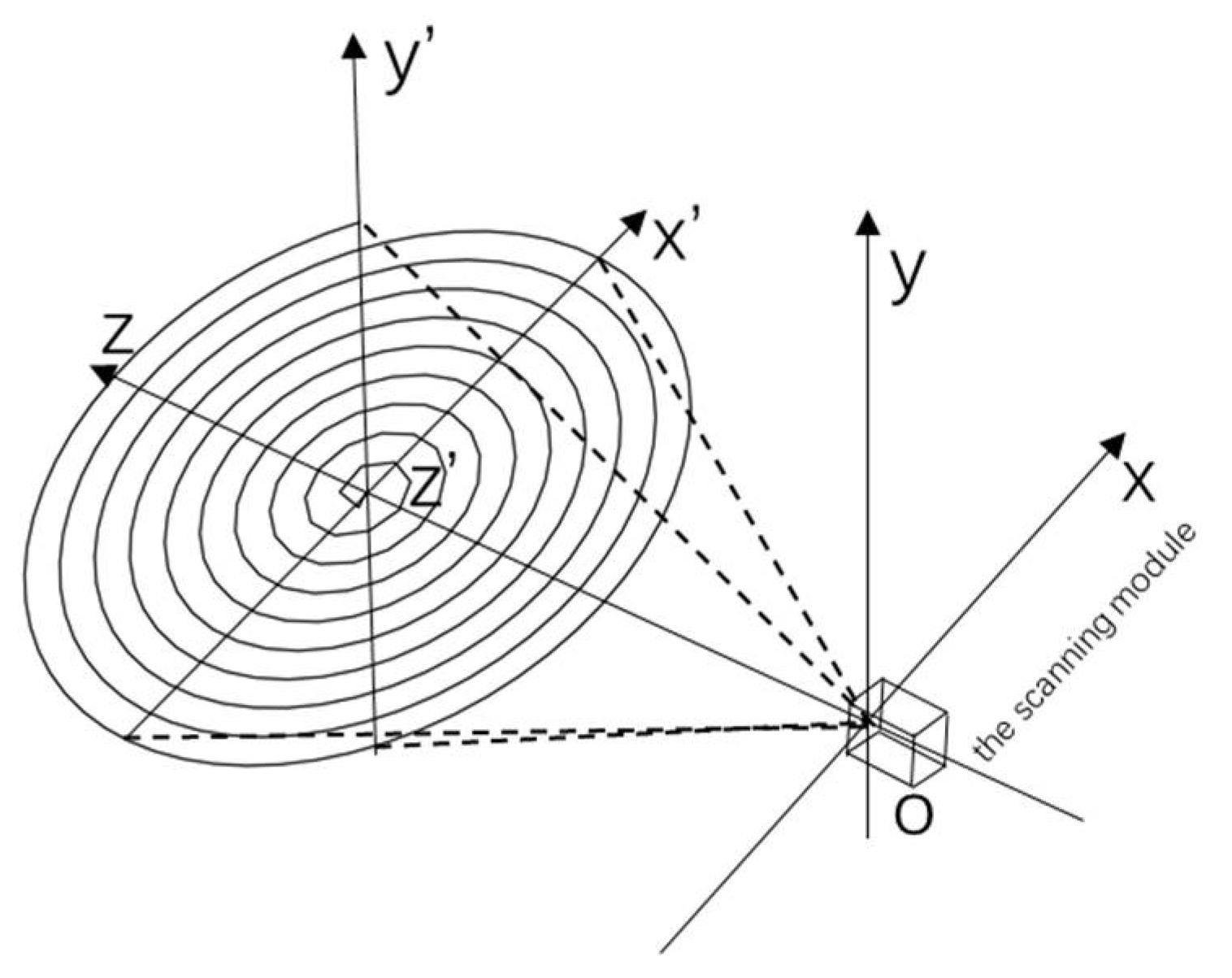
There are some main scanning methods, such as spiral scanning and raster scanning. Different scanning modes have different characteristics. Among them, linear spiral scanning has the advantage of high capture probability. This scanning method scans from the high probability position to the least likely location and dwells on each spot for a constant duration. Moreover, the scanning capture efficiency is relatively high [28,29,30,31]. The geometry diagram of spiral scanning is shown in Figure 4.

The constant linear velocity spiral scanning mode has a fixed expression [29], which can be easily written into the scanning system’s DSP control to realize spiral scanning. The equations are extended as follows:

$$V_r=\sqrt{\frac{\left(1-F\right)·{\theta }_{1/\mathrm{e}}^2}{2\cdot \pi \cdot t\cdot T_{dwell}}},$$

(6)

$$V_{\theta }=\sqrt{\frac{2\cdot \pi }{\left(1-F\right)\cdot t\cdot T_{dwell}}},$$

(7)

$${\theta }_{msa}=\left(1-F\right)\cdot {\theta }_{1/e}\cdot M,$$

(8)

$$T_{scan}=\frac{2\cdot \pi \cdot M\cdot {\theta }_{msa}\cdot T_{dwell}}{{\theta }_{1/e}}=2\cdot \pi \cdot (1-F)M^2\cdot T_{dwell},$$

(9)

where $V_r$ and $V_{\theta }$ is the radial velocity and angular velocity of the scanning laser, respectively; $F$ is the overlap factor of the laser spot, which is generally 0.29 to cover all scanning areas and prevents missing scanning [32]; ${\theta }_{1/e}$ is the divergence angle of the laser beam; $M$ represents the number of rings and determines the maximum radius of the scan; ${\theta }_{\mathrm{msa}}$ is the maximum angle of the laser scan deviating from the center of the scan; $t$ is the time from 0 to $T_{scan}$; $T_{dwell}$ is the expression for the laser dwell time on the target, which is actually the scan time corresponding to the adjacent spot angle ${\theta }_{1/e}/2$, $T_{scan}$ is the total scan time from initial point to the searching end.

Then the $X$ and $Y$ angle coordinate of the center of the laser spot by a linear spiral scanning is given. At the same time, for the classical scanning system parameters, after a very short scanning time, the linear velocity, $V$, is also expressed. Their expressions are as follows:

$$X=V_r\cdot t\cdot cos(V_{\theta }\cdot t),$$

(10)

$$Y=V_r\cdot t\cdot sin(V_{\theta }\cdot t),$$

(11)

$$V=\frac{{\theta }_{1/e}}{2\cdot T_{dwell}},$$

(12)

Suppose the time interval of the output angle information in the scanning system is $T_{out}$, which is the time used for the overlap factor between two laser spots and is related to the overlap factor and the laser dwell time. In addition, assuming that the target position changes slightly within $T_{out}$. In order to extract the target signals for the single photon detection, multiple pulses need to be accumulated within $T_{out}$. Then we have the following:

$$T_{out}=\frac{\left(1-F\right)\cdot {\theta }_{1/e}}{V}=2\cdot T_{dwell}\cdot \left(1-F\right)=\frac{N}{PRF},$$

(13)

where $PRF$ is the laser pulse repetition frequency, and $N$ is the number of accumulated pulses.

Combining Equations (9), (13), and (14), we see that the relationship between the total scan time and the number of accumulated pulses is given by the following:

$$T_{scan}=\frac{\pi \cdot M^2\cdot N}{PRF},$$

(14)

According to Equation (15), under the condition that the number of rings and laser pulse repetition frequency are fixed, the smaller number of accumulated is, the shorter the time it takes to scan a frame is, and the stronger its ability to capture and track the target is [29]. Thus, under the guarantee of high detection probability and low false-alarm probability, the number of accumulated pulses should be small.

3.3. Derivation and Analysis for the Position of the Target

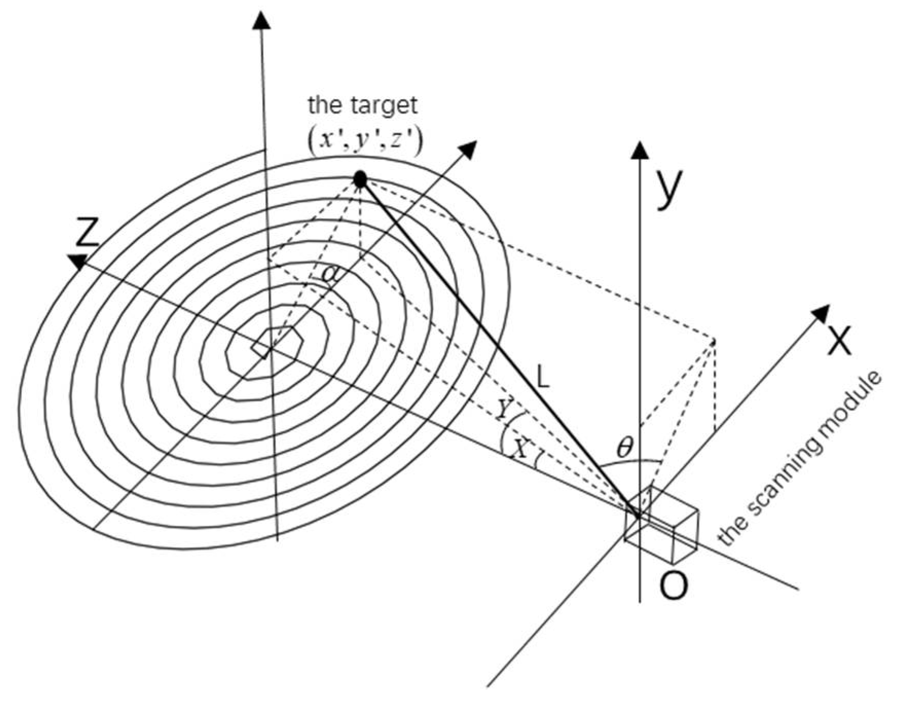
According the scanning model, we can get the three-dimensional coordinates and orientation of the captured target. As shown in Figure 5, the three-dimensional coordinates of the target are as follows:

$$\begin{array}{c}{x}^{\prime }=\frac{L}{\sqrt{1+{tan}^2(X)+{tan}^2(Y)}}\cdot \tan (Y),\\ y^{\prime }=\frac{L}{\sqrt{1+{tan}^2(X)+{tan}^2(Y)}}\cdot tan(X),\\ z^{\prime }=\frac{L}{\sqrt{1+{tan}^2(X)+{tan}^2(Y)}},\end{array}$$

(15)

where the $X$ and $Y$ are the angle coordinate of the center of the laser spot by a linear spiral scanning, and $L$ is the distance of the echo target from the single photon detection. In the formula written by DSP, X represents the vertical direction of the FSM, and Y represents the horizontal direction of the fast mirror, so coordinate correction is carried out here.

When the target is extended, it is possible to measure multiple points of the target. Thus, the centroid algorithm is used to obtain the centroid of the target, which is given by the following:

$$x_0=\frac{{\sum }_{i=1}^n{k}_i\cdot x_i^{}{}^{\prime }}{{\sum }_{i=1}^n{k}_i},y_0=\frac{{\sum }_{i=1}^n{k}_i\cdot y_i^{}{}^{\prime }}{{\sum }_{i=1}^n{k}_i},z_0=\frac{{\sum }_{i=1}^n{k}_i\cdot z_i^{}{}^{\prime }}{{\sum }_{i=1}^n{k}_i},$$

(16)

$$n=|\frac{T_{scan}}{T_{out}}+1|,$$

(17)

where $n$ is the number of points detected in a scan cycle, which is also called the number of 3D imaging pixels; || means rounding down; and the $k_i$ is the weighting factor. When the detected distance is less than the system threshold, $k_i$ is equal to 0; otherwise, $k_i$ equals 1. In fact, for a single target in the airspace, we do not consider the background of the target.

The distance, azimuth, and pitch of the centroid of the target are as follows:

$$\begin{array}{c}{L}_0=\sqrt{x_0^2+y_0^2+z_0^2},\\ \alpha =arctan(\frac{y_0}{x_0}),\\ \theta =arcsin(\frac{z_0}{L_0}),\end{array}$$

(18)

At the same time, the scanning module points to the centroid of the target, and the angle coordinates of the scanning center are changed, as given by the following:

$$\begin{array}{c}{X}_0=arctan(\frac{x_0}{z_0}),\\ Y_0=arctan(\frac{y_0}{z_0}),\end{array}$$

(19)

4. Strategy and Simulation Process of Target Tracking and Analysis of Experimental Results, and the Ability of Tracking and Detection

4.1. Tracking and Ranging Strategy of Target and the Simulation Process

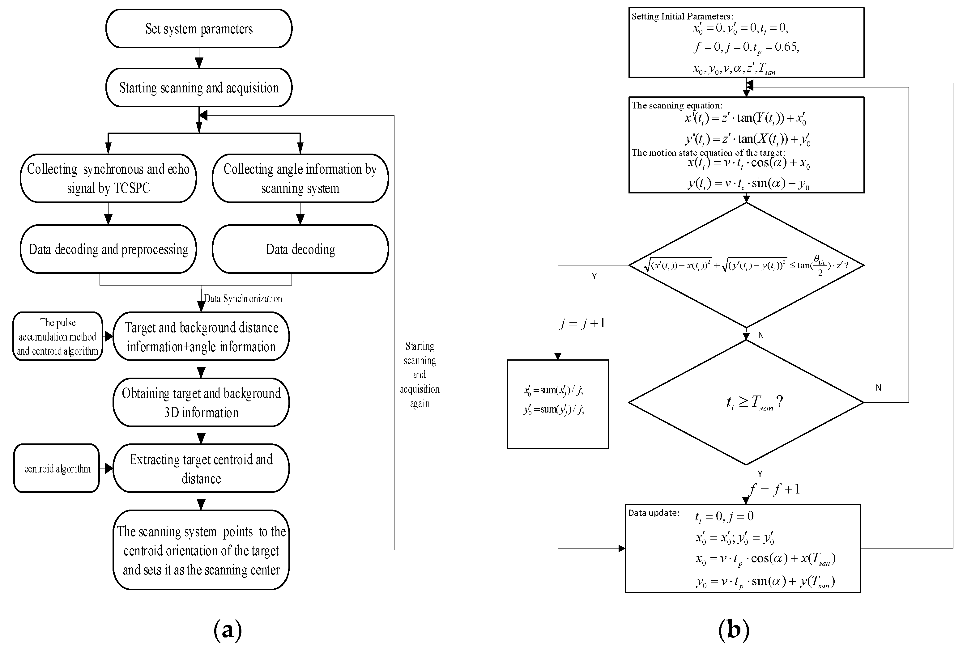
The target tracking flowchart is shown in Figure 6a. Firstly, according to the analysis in Section 3, the system parameters are set. Then the signal processing control module simultaneously controls TCSPC and the scanning module to collect laser echo information and corresponding angle information, and decodes and preprocesses the collected data. Next, the signal processing control module combines echo distance information of the target or background by using the pulses accumulation algorithm and centroid algorithm with the angle information to obtain and display the three-dimensional information of the target and background. Finally, the system obtains the centroid orientation and ranging of the target obtained by using the centroid algorithm. Then the scanning module points to the target centroid and sets its orientation as the spiral line scanning center. By scanning and capturing the target continuously, the system can track the target in real time. As shown in Figure 6b, the simulation process of the APT of the target is presented. To simplify the model analysis, a point target is defined as the target in the simulation. Simultaneously, suppose that the target is captured on a plane of space. In Figure 6b, $j$ represents the number of times the target is captured in a frame, $f$ is the number of frames scanned, and $t_p$ is the time of processing data and about 0.65 s in the experiment. Moreover, $x_0^{\prime }$ and $y_0^{\prime }$ are the initial position of the scan center, and $x_0$ and $y_0$ are the initial position of the target with a velocity of $v$ and the azimuth of $\alpha$; $z^{\prime }$ is the distance from the center of the FSM to the moving plane of the target. In addition, due to the spot overlap, the target may be captured multiple times in a frame. Here we consider that the average is taken to update the scanning center in the process.

4.2. Simulation and Experimental Results and Analysis

In order to verify the feasibility of the system based on single photon detection, the experiment was carried out by setting reasonable parameters. In this system, the output average power is 0.197 mw, and a histogram that was produced by 5000 cycles was analyzed for the static target at about 3.26 m. It is found that the mean number of signal echo photons is about 10, which means that the average received power is 9.34 × 10⁻¹⁵ W with the repetition frequency of 5 khz, the peak power is 1.868×10⁻¹⁰ W with the pulse width of 10 ns, and the average number of noise photons is 8.5 × 10⁻⁶ in each time bin (10 ns) for the SPD with about 7% quantum efficiency to 1064 nm laser. Meanwhile, the ranging resolution is about 30 cm by analyzing the full width at half maximum (FWHM) of the weak echo signal. According to the analysis in Section 3, to ensure high detection probability about 1 and low false-alarm probability less than 1 ×10⁻⁵ and considering the fluctuation of the number of echo photons and short total scan time, the number of accumulated pulses 14 and the threshold of the recognition target 1 were chosen for the experiment. The main input system parameters are shown in

Table 1. Main input parameters of the lidar system.

Parameter	Value
Pulse repetition frequency ($PRF$)	5 Khz
Divergence angle (${\theta }_{1/e}$)	1.9 mrad
Number of accumulated pulses ($N$)	14
Threshold of the recognition target ($k_{th}$)	1
Overlap factor ($F$)	0.29
Number of rings ($M$)	10
Time interval of the output angle ($T_{out}$)	2.8 ms
Total scan time ($T_{scan}$)	879.6 ms

.

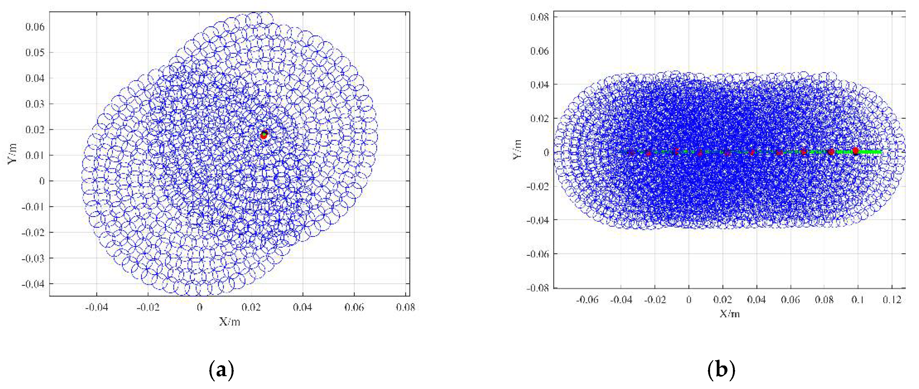
According to the Table 1 and Equation (8), ${\theta }_{\mathrm{msa}}$ is 0.01349 rad. Thus, the scanning field of view (FoV) is 0.02698 rad, and the lateral resolution, which is related to the overlap factor and the divergence, is $\left(1-F\right)\cdot {\theta }_{1/e}$, and its theoretical value is about 1.349 mrad. The number of 3D imaging pixels is about 315, as seen in Table 1 and Equation (17). Meanwhile, simulation parameters are set according to Table 1 and the target’s distance and state. The simulation of the APT of a point target is shown in Figure 7. In this simulation, the blue circle and green dot represent the scanning light spot and the trajectory of the dynamic target, respectively. Moreover, the red dot and black dot represent the calculated position and actual position of the target captured, respectively, and the angular error is less than 1.349 mrad. The static target and dynamic target are scanned with 2 frames and 10 frames, respectively. Furthermore, it can be found that the simulation provides theoretical guidance and visual process for actual capture and tracking experiments.

The target tracking and ranging experiment is carried out in conditions of a weak echo signal in indoor lab. A background consistent with the reflectivity of the target is added behind the target to better highlight the trajectory of the helical scan capture and tracking, and the process of target tracking. The distance between them is about 41 cm. The initial purpose of our system is to track and detect a single target in the airspace, and it usually does not consider to distinguish two targets. Therefore, in the experiment, we can set the appropriate system threshold, z’, from 3.14 to 3.34 m and extract the target centroid by analyzing the previous distance information of the target and the background. Only after extracting the centroid can the system carry out the next APT.

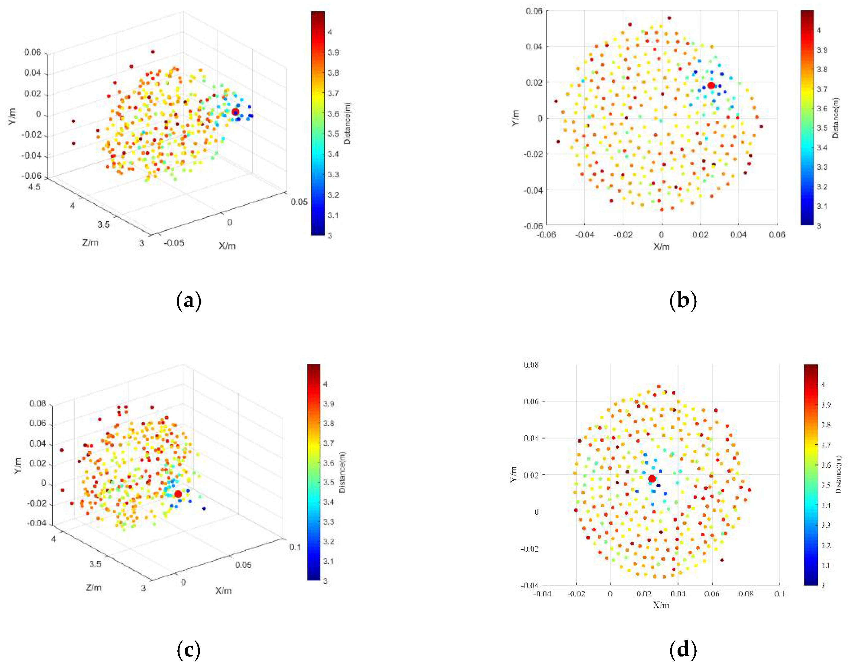
The static target is scanned, captured, and pointed, and the results are shown in Figure 8a–d, which display the 3D information of the background and target scanned by the spiral line for one experiment. The results show that the coordinates and distance of the target centroid (the red dot) are (0.0257099, 0.0181003, and 3.26308 m) and 3.26323 m, respectively, before pointing the target. Moreover, they are (0.0246935, 0.0178932, and 3.26281 m) and 3.26296 m, respectively, after pointing to the target. It proves that the difference of the distance is small—about 0.00027 m—and the scanning center points to the target. Figure 8e shows that the scanning center does not coincide with the target before pointing to the target. Figure 8f shows that the scanning center coincides with the target after pointing to the target. The experiment is repeated 10 times, which is shown in

Table 2. Coordinates, distance, azimuth, and pitch of the target centroid.

No.	Before Pointing to the Target							After Pointing to the Target
	x0/m	y0/m	z0/m	L0/m	α/rad	θ/rad		x0/m	y0/m	z0/m	L0/m	α/rad	θ/rad
1	0.0257	0.0181	3.2631	3.2632	0.6134	1.5612		0.0247	0.0179	3.2628	3.2630	0.6271	1.5612
2	0.0239	0.0223	3.2542	3.2544	0.7503	1.5606		0.0153	0.0188	3.2464	3.2465	0.8876	1.5634
3	0.0247	0.0156	3.2797	3.2798	0.5619	1.5619		0.0251	0.0214	3.2709	3.2710	0.7062	1.5609
4	0.0188	0.0215	3.2582	3.2584	0.8536	1.5619		0.0222	0.0234	3.2374	3.2375	0.8106	1.5609
5	0.0229	0.0216	3.2699	3.2701	0.7544	1.5609		0.0300	0.0220	3.2909	3.2911	0.6324	1.5595
6	0.0191	0.0222	3.2760	3.2761	0.8603	1.5619		0.0234	0.0147	3.2643	3.2644	0.5622	1.5622
7	0.0188	0.0233	3.2572	3.2573	0.8915	1.5615		0.0245	0.0189	3.2415	3.2416	0.6578	1.5612
8	0.0188	0.0196	3.2572	3.2573	0.8050	1.5622		0.0276	0.0188	3.2283	3.2285	0.5983	1.5605
9	0.0204	0.0234	3.2467	3.2469	0.8530	1.5612		0.0260	0.0218	3.2646	3.2648	0.6973	1.5606
10	0.0246	0.0174	3.2717	3.2718	0.6157	1.5615		0.0246	0.0205	3.3093	3.3095	0.6937	1.5610
Mean	0.0218	0.0205	3.2634	3.2635	0.7559	1.5615		0.0243	0.0198	3.2616	3.2618	0.6873	1.5611
Standard Deviation	0.0027	0.0026	0.0100	0.0100	0.1133	0.0005		0.0037	0.0024	0.0236	0.0236	0.0932	0.0010

. In the static target acquisition and pointing experiment, the average distance of the target is 3.263513 and 3.261791 m, respectively, which is consistent with the theoretical value of 3.26 m within allowable error and the error is less than 0.0035 m. The standard deviation of the target distance is less than 0.0236 m. Furthermore, the azimuth and pitch of the centroid of the target are less than 0.113269 and 0.000979 rad, respectively. Meanwhile, these results of Table 2 present that errors of the parameters before and after pointing to the target are small and proves that the system has acquisition and pointing capability in conditions of a weak echo signal.

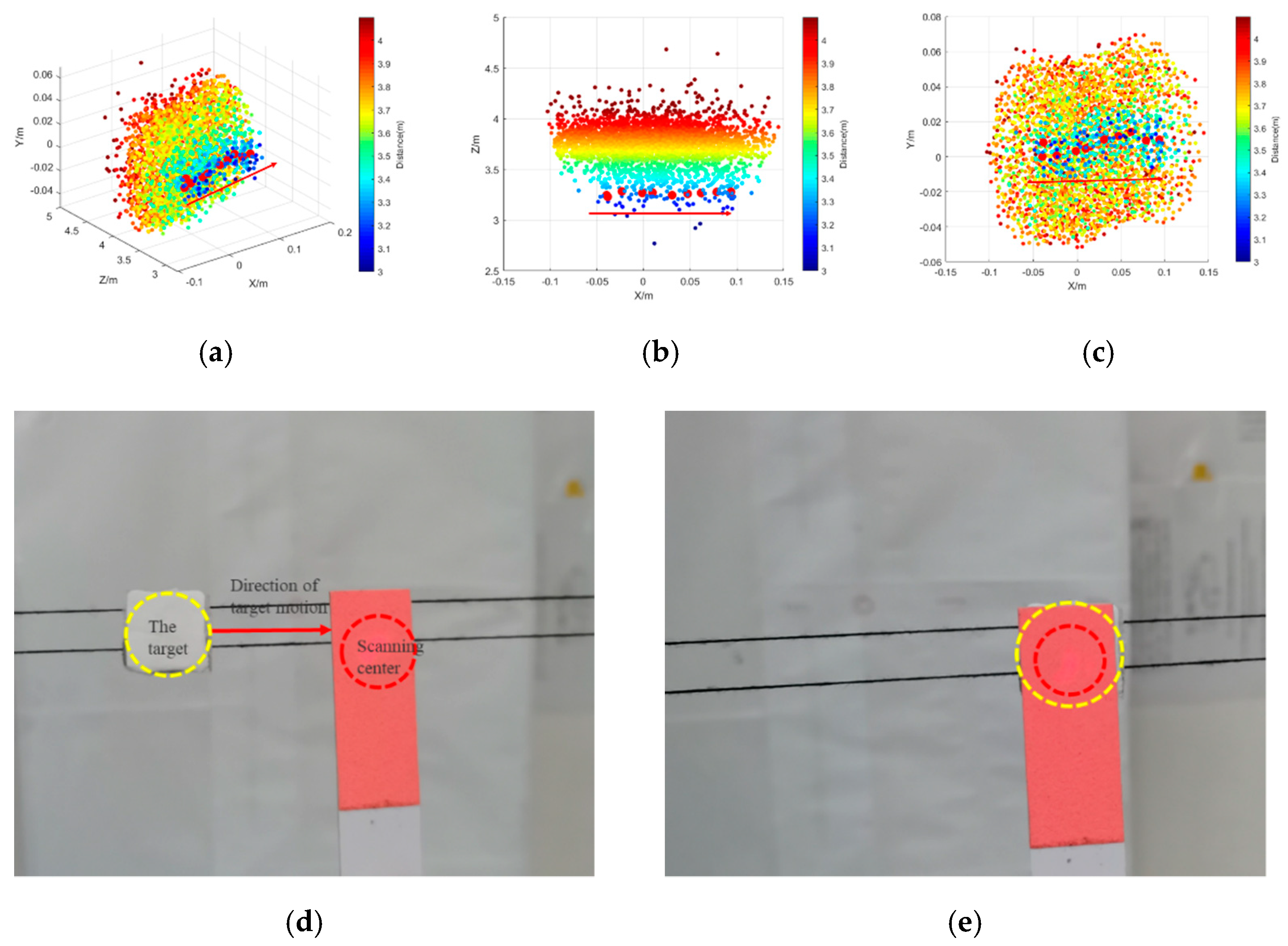
The dynamic target is scanned, captured, and tracked, and the results are shown in Figure 9. The lateral velocity of the target is about 1 cm/s at 3.26 m, and the angular velocity is about 3.067 mrad/s. The target is at the edge of the scan area and the target does not move horizontally into the scan area until the scan begins. A total of 10 frames are scanned, and the result is refreshed in each frame to achieve real-time tracking of the target. The red arrow is the direction of the target motion, and the red dot indicates that the target centroid is obtained by scanning in each frame. As shown in

Table 3. Coordinates and distance of the target centroid.

No.	1					2
	x0/m	y0/m	z0/m	L0/m		x0/m	y0/m	z0/m	L0/m
1	−0.0396	0.0000	3.2461	3.2463		−0.0399	−0.0033	3.2532	3.2534
2	−0.0383	0.0082	3.2305	3.2307		−0.0298	0.0066	3.2540	3.2541
3	−0.0232	0.0007	3.2840	3.2841		−0.0136	0.0069	3.2596	3.2597
4	−0.0014	0.0032	3.2678	3.2678		0.0068	0.0059	3.2756	3.2756
5	0.0096	0.0047	3.2723	3.2724		0.0180	0.0076	3.2869	3.2869
6	0.0306	0.0097	3.2462	3.2464		0.0389	0.0044	3.2579	3.2581
7	0.0473	0.0118	3.2597	3.2601		0.0491	0.0114	3.2648	3.2652
8	0.0616	0.0142	3.2681	3.2687		0.0693	0.0169	3.2387	3.2395
9	0.0784	0.0093	3.2788	3.2797		0.0861	0.0033	3.2468	3.2480
10	0.0937	0.0098	3.2785	3.2799		0.0961	0.0078	3.2721	3.2735

and Figure 9a–c, we can find that the target centroid moves horizontally about 13 cm but unstably by the values of $x_0$ and $y_0$. The values of $z_0$ and $L_0$ indicate that the target has no absolute lateral movement and is affected by the ranging accuracy; moreover, the mean of $z_0$ is about 3.262076 m, which is consistent with the theoretical value of 3.26 m within allowable error. There are ten centroid points for a total of 10 frames in (Figure 9a–c), which show the target is tracked in real time. Figure 9d shows the image before tracking the target. When the target stops moving, the system’s scan center finally points to the target, which is shown in Figure 9e. Meanwhile, we have a second experiment under the same conditions in Table 3. These data are consistent with the first experiment data and prove that the system has the tracking ability of the target in conditions of a weak echo signal.

As shown in Figure 7, Figure 8 and Figure 9, it is found that there is a little difference between the actual tracking of the dynamic target and the simulation, which is caused by the instability of the target motion, the ranging accuracy, and the fact that the target stops before the end of the scan, etc. However, the experiment is consistent with the simulation as a whole. Simultaneously, by combining tabular data, we can find that the system has acquisition pointing and tracking capability based on single photon detection and have an excellent performance to realize the acquisition, pointing and ranging of a static target, and the APTR of a dynamic target with a lateral angular velocity is about 3.067 mrad/s, especially in conditions of a weak echo signal. Moreover, weak echo detection is the basis of the long-distance detection.

4.3. Analysis of Tracking and Detection Capability

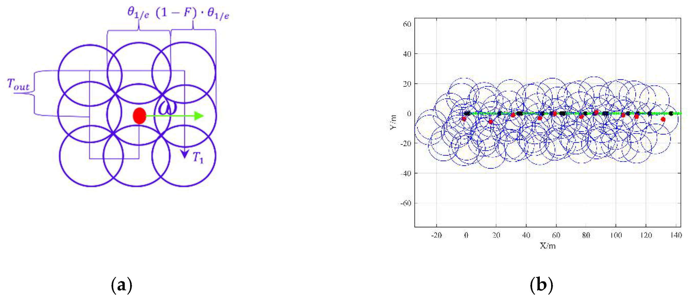
In Section 4.1 and Section 4.2, we found that the target tracking and ranging system based on single photon detection has a good effect when the number of echo photons is about 10 weak echo signals and the noise is relatively weak, which verifies the ability of weak echo tracking and ranging based on the combination of single photon detection and scanning system. In order to show the fast long-distance tracking and detection ability based on this system, we make a further analysis of the theory. Since the spiral scanning in this experiment is relatively complex, we use the raster spiral scan as the equivalent substitute for the simplifying geometric analysis, which is shown in Figure 1a. Spiral scanning has a higher probability of capture when the target distribution model obeys the Gaussian distribution, and the closer it is to the center, the faster the scanning will be and the higher the scanning efficiency will be. Therefore, on the basis that the target has been captured, the smaller the scanning range is set, the stronger the ability of capturing and tracking is. However, the number of rings should be greater than or equal to 1, so that the position of the target can be determined. In order to verify the tracking ability, the lateral angular velocity of the target motion should meet the formula: $w·T_1\le \left(1-F\right){\theta }_{1/e}$ and $T_1$ is the time to scan the first lap. Only in this way can the target not escape from the scanning area. Moreover, the movement distance of the target can not be more than the size of a spot and multiple pulses can be accumulated on the target within the $T_{out}$ time. It is assumed that the approximate area or uncertain area information of the target can be obtained by other methods.

The parameters of the designed system and the target are shown in

Table 4. The design parameters of the lidar system and the target.

Parameter	Value
Energy of the laser ($E_t$)	$6\times {10}^{-3}$ J
Laser wavelength ($\lambda$)	1064 nm
Laser pulse width ($T_t$)	2 ns
Laser divergence angle (${\theta }_{1/e}$)	$200\times {10}^{-6}$ rad
Effective receiving area ($A_r$)	$0.04{\mathrm{m}}^2$
Atmospheric transmittance (${\tau }_a$)	0.7
Optical efficiency of a lunch system (${\eta }_t$)	0.9
Optical efficiency of a receiving system (${\eta }_r$)	0.8
Reflection efficiency of the target ($\rho$)	0.3
Effective area of the target ($A_t$)	1${\mathrm{m}}^2$

, and they are in line with the actual project. The number of received mean echo photons from the target is about 10.8 in a time bin (2 ns) at 100 km by the following equation:

$$n_s=\frac{E_t·{\eta }_t·{\eta }_r·{\tau }_r^2·\rho ·A_t·A_r}{\pi ·Z^4{\theta }_{1/e}^2}·\frac{\lambda }{h·c},$$

(20)

where $h$ and $c$ are the Planck’s constant and the velocity of light, respectively; $Z$ is the distance between the target and the system.

Assume that the noise photons count rate is 1 Mcps, and the received average number of noise photons n is 2 × 10⁻³ in a time bin (2 ns). When the number of accumulated pulses 10 and the threshold of the recognition target 1 are chosen for the design the detection probability and false-alarm probability are about 99.946% and 0.139%, respectively, by the Equations (4) and (5) (the dead time is 45 ns). It indicates that the target can be detected at a distance of 100 km. In fact, the number of accumulated pulses can fluctuate in a small range without no considerable impact on high detection probability.

Under detectable conditions, we find that there are 9 probe points needed to complete the first circle with a raster spiral scan. To meet detection requirements, each point stays for about 2 ms and there are the accumulation of about 10 pulses. We can find that $T_1=9·T_{out}=18 \mathrm{m}\mathrm{s}$, and the target with a lateral angular velocity of 7.8889 mrad/s can be captured and tracked at F = 0.29 and ${\theta }_{1/e}=200·{10}^{-6} \mathrm{r}\mathrm{a}\mathrm{d}$. It means that the system under this research method has the ability to track a target with a lateral velocity of 788.89 m/s at a long distance of 100 km which is show in Figure 10b. Moreover, the angular error is less than $142·{10}^{-6} \mathrm{r}\mathrm{a}\mathrm{d}$. Here, a frame is about 18 ms and the amount of data is relatively small, and assume that the data-processing time is negligible. The number of accumulated pulses can be up to 10 or more for Tout = 2 ms by the macro pulse method [13,33]. Meanwhile, the ability of the target tracking and detecting also can be improved. And, the Equation (13) needs to be partially modified as:

$$T_{out}=\frac{\left(1-F\right)\cdot {\theta }_{1/e}}{V}=2\cdot T_{dwell}\cdot \left(1-F\right)=\frac{1}{PR{F}_M},$$

(21)

where, $PR{F}_M$ is the macro pulse period, which can solve the range ambiguity. In the macro pulse period, we can reasonably set N sub-pulses and accumulate them by compensating the delay of the sub-pulses. In addition, the detection requirements also can be met by using pseudo-random or true random coded [34,35,36] and $PR{F}_M$ is changed to the period of a random sequence.

5. Conclusions

In order to achieve the APTR of the non-cooperative target in conditions of a weak echo signal, we designed an APTR lidar system. The system is composed of the signal processing control module, single photon detection module, and scanning module. Moreover, the system can avoid some defects caused by the devices, such as CCD, CMOS, four-quadrant detectors, and array detectors for measuring target azimuth. In this paper, we analyzed the relationship between the number of accumulated pulses and the detection and false-alarm probabilities, and the total scan time by using a spiral scanning and single photon detection models in detail. Furthermore, we also derive the three-dimensional coordinates and orientation of the target. Then the target tracking and ranging strategy and the simulation of APT of a target were designed. The pulse accumulation method and centroid algorithm were applied to ensure the target detection capability. Finally, we completed the preliminary functional verification experiment and select the appropriate number of accumulated pulses to realize the APTR of the non-cooperative target in conditions of about ten echo photons. Meanwhile, through further theoretical analysis, it was proven that the system can have the ability of the fast long-distance non-cooperative target tracking and ranging in conditions of a weak echo signal. Moreover, it provides a new idea for fast long-distance non-cooperative target tracking and ranging only by using a single-point single photon detector. It is meaningful to be applied to the active tracking and ranging of an airborne target.

References

- Bachman, C.G. Laser Radar Systems and Techniques; Artech House: Dedham, UK, 1979. [Google Scholar]
- Pfennigbauer, M.; Mbius, B.; Carmo, J.P.D. Echo Digitizing Imaging Lidar for Rendezvous and Docking. In Proceedings of the Laser Radar Technology and Applications XIV, SPIE Defense, Security, and Sensing, Orlando, FL, USA, 30 April 2009. [Google Scholar]
- Ferraro, M.S.; Mahon, R.; Rabinovich, W.S.; Freeman, W.T.; Murphy, J.L.; Goetz, P.G.; Burris, H.R.; Moore, C.I.; Thomas, L.M.; Clark, W.R. InGaAs Avalanche Photodiode Arrays for Simultaneous Communications and Tracking. In Proceedings of the Free-Space and Atmospheric Laser Communications XI, San Diego, CA, USA, 24–25 August 2011; p. 81620D. [Google Scholar]
- Greene, B.; Gao, Y.; Moore, C.; Wang, Y.; Boiko, A.; Ritchie, J.; Sang, J. Laser Tracking of Space Debris. In Proceedings of the 13th International Workshop on Laser Ranging Instrumentation, Washington, DC, USA, 10 October 2002. [Google Scholar]
- Wu, C.; Xing, W.; Feng, Z.; Xia, L. Moving Target Tracking in Marine Aerosol Environment with Single Photon Lidar System. Opt. Lasers Eng. 2020, 127, 105967. [Google Scholar] [CrossRef]
- Jimenez, A.; Ceres, R.; Seco, F. A Laser Range-finder Scanner System for Precise Manoeuver and Obstacle Avoidance in Maritime and Inland Navigation. In Proceedings of the Proceedings Elmar-2004, 46th International Symposium on Electronics in Marine, Zadar, Croatia, 16–18 June 2004; pp. 101–106. [Google Scholar]
- Kim, B.H.; Khan, D.; Choi, W.; Kim, M.Y. Real-time Counter-UAV System for Long Distance Small Drones using Double Pan-tilt Scan Laser Radar. In Proceedings of the Laser Radar Technology and Applications XXIV, SPIE Defense + Commercial Sensing, Baltimore, MD, USA, 2 May 2019; p. 110050C. [Google Scholar]
- Leigh-Lancaster, C.J.; Shirinzadeh, B.; Koh, Y.L. Development of a Laser Tracking System. In Proceedings of the Proceedings Fourth Annual Conference on Mechatronics and Machine Vision in Practice, Toowoomba, Australia, 23–25 September 1997; pp. 163–168. [Google Scholar]
- Buller, G.; Collins, R. Single-photon Generation and Detection. Meas. Sci. Technol. 2009, 21, 012002. [Google Scholar] [CrossRef]
- Du, X.; Xing, J.C.; Huang, H. Method to Simulate the Object Tracking with Photon-counting Laser Ranging System. Opt. Eng. 2015, 54, 114103. [Google Scholar] [CrossRef]
- Castleman, A.W.; Toennies, J.P.; Zinth, W. Advanced Time-Correlated Single Photon Counting Techniques; Springer: Berlin/Heidelberg, Germany, 2005. [Google Scholar]
- Becker, W.; Bergmann, A. Multi-Dimensional Time-Correlated Single Photon Counting. In Reviews in Fluorescence 2005; Geddes, C.D., Lakowicz, J.R., Eds.; Springer: Boston, MA, USA, 2005; pp. 77–108. [Google Scholar]
- Yu, Y.; Liu, B.; Chen, Z.; Li, Z.K. A Macro-Pulse Photon Counting Lidar for Long-Range High-Speed Moving Target Detection. Sensors 2020, 20, 2204. [Google Scholar] [CrossRef] [PubMed] [Green Version]
- Massa, J.S.; Buller, G.S.; Walker, A.C.; Cova, S.; Umasuthan, M.; Wallace, A.M. Time-of-flight Optical Ranging System based on Time-correlated Single-photon Counting. Appl. Opt. 1998, 37, 7298–7304. [Google Scholar] [CrossRef] [PubMed] [Green Version]
- Xue, L.; Zhang, L.; Zhang, S.; Li, M.; Kang, L.; Chen, J.; Wu, P. Satellite Laser Ranging using Superconducting Nanowire Single-photon Detectors at 1064 nm Wavelength. Opt. Lett. 2016, 41, 3848. [Google Scholar] [CrossRef] [PubMed]
- Blazej, J.; Prochazka, I.; Kodet, J. Photon Counting Detector for High-repetition-rate Optical Time Transfer Providing Extremely High Data Yield. Opt. Eng. 2014, 53, 081903. [Google Scholar] [CrossRef] [Green Version]
- Kong, H.J.; Kim, T.H.; Jo, S.E.; Oh, M.S. Smart Three-dimensional Imaging Ladar using Two Geiger-mode Avalanche Photodiodes. Opt. Express 2011, 19, 19323. [Google Scholar] [CrossRef] [PubMed]
- Liu, B.; Yu, Y.; Jiang, S. Review of Advances in LiDAR Detection and 3D Imaging. Guangdian Gongcheng/Opto-Electron. Eng. 2019, 46, 2019–2065. [Google Scholar]
- Yang, Y.; Bo, L.; Zhen, C. Analyzing the Performance of Pseudo-random Single Photon Counting Ranging Lidar. Appl. Opt. 2018, 57, 7733. [Google Scholar]
- Li, C.; Wang, S.; Huo, L.; Wang, Y.; Liang, K.; Yang, R.; Han, D. Position Sensitive Silicon Photomultiplier With Intrinsic Continuous Cap Resistive Layer. IEEE Trans. Electron Devices 2014, 61, 3229–3232. [Google Scholar] [CrossRef]
- Zappa, F.; Lacaita, A.; Cova, S.; Lovati, P. Counting, Timing, and Tracking with a Single-photon Germanium Detector. Opt. Lett. 1996, 21, 59–61. [Google Scholar] [CrossRef] [PubMed]
- De-Bur, V.; Terekhov, A.; Kosolobov, S.; Sheibler, H.; Plokhotnichenko, V. Position-Sensitive Detector with GaAs Photocathode and High Time Resolution; AIP Conference Proceedings 984; American Institute of Physics: College Park, MD, USA, 2008; pp. 186–193. [Google Scholar]
- Fouche, D.G. Detection and False-alarm Probabilities for Laser Radars that Use Geiger-mode Detectors. Appl. Opt. 2003, 42, 5388–5398. [Google Scholar] [CrossRef] [PubMed]
- Gatt, P.; Johnson, S.; Nichols, T. Geiger-mode Avalanche Photodiode Ladar Receiver Performance Characteristics and Detection Statistics. Appl. Opt. 2009, 48, 3261–3276. [Google Scholar] [CrossRef]
- Johnson, S.; Gatt, P.; Nichols, T. Analysis of Geiger-mode APD Laser Radars. In Proceedings of the Laser Radar Technology and Applications VIII, AeroSense 2003, Orlando, FL, USA, 21 August 2003. [Google Scholar]
- Chen, Z.; Liu, B.; Guo, G. Adaptive Single Photon Detection under Fluctuating Background Noise. Opt. Express 2020, 28, 30199. [Google Scholar] [CrossRef] [PubMed]
- O’Connor, D. Time-correlated Single Photon Counting; Academic Press: Cambridge, MA, USA, 1984. [Google Scholar]
- Scheinfeild, M.; Kopeika, N.S.; Melamed, R. Acquisition System for Microsatellites Laser Communication in Space. In Proceedings of the Free-Space Laser Communication Technologies XII, Symposium on High-Power Lasers and Applications, San Jose, CA, USA, 2 May 2000; pp. 166–175. [Google Scholar]
- Hindman, C.; Robertson, L. Beaconless Satellite Laser Acquisition-modeling and Feasability. In Proceedings of the IEEE MILCOM 2004 Military Communications Conference, Monterey, CA, USA, 31 October–3 November 2004. [Google Scholar]
- Teng, Y.; Zhang, M.; Tong, S. The Optimization Design of Sub-regions Scanning and Vibration Analysis for Beaconless Spatial Acquisition in the Inter-satellite Laser Communication System. IEEE Photonics J. 2018, 10, 1–11. [Google Scholar] [CrossRef]
- Zhang, M.; Li, B.; Tong, S. A New Composite Spiral Scanning Approach for Beaconless Spatial Acquisition and Experimental Investigation of Robust Tracking Control for Laser Communication System with Disturbance. IEEE Photonics J. 2020, 12, 1–12. [Google Scholar] [CrossRef]
- Xin, L.; Quanyou, S.; Jing, M.; Siyuan, Y.; Liying, T. Spatial Acquisition Optimization based on Average Acquisition Time for Intersatellite Optical Communications. In Proceedings of the 2010 Academic Symposium on Optoelectronics and Microelectronics Technology and 10th Chinese-Russian Symposium on Laser Physics and Laser TechnologyOptoelectronics Technology (ASOT), Harbin, China, 28 July–1 August 2010; pp. 244–248. [Google Scholar]
- Liu, B.; Jiang, S.; Yu, Y.; Chen, Z. Macro/sub-pulse Coded Photon Counting LIDAR. Opto-Electron. Eng. 2020, 47, 99–109. [Google Scholar]
- Hiskett, P.A.; Parry, C.S.; Mccarthy, A.; Buller, G.S. A Photon-counting Time-of-flight Ranging Technique Developed for the Avoidance of Range Ambiguity at Gigahertz Clock Rates. Opt. Express 2009, 16, 13685–13698. [Google Scholar] [CrossRef]
- Krichel, N.J.; Mccarthy, A.; Buller, G.S. Resolving Range Ambiguity in a Photon Counting Depth Imager Operating at Kilometer Distances. Opt. Express 2010, 18, 9192–9206. [Google Scholar] [CrossRef] [PubMed]
- Liu, B.; Yu, Y.; Chen, Z.; Han, W. True Random Coded Photon Counting Lidar. Opto-Electron. Adv. 2020, 3, 190044. [Google Scholar] [CrossRef]
Figure 1.
(a) Block diagram of APTR system based on single photon detection; (b) the experimental platform of APTR system based on single photon detection.
Figure 2.
Detection probability and false-alarm probability: (a) influence of number of accumulated pulses on detection probability and false-alarm probability ( = 10, = 8.5 × 10⁻⁶, = 1, 2, 3, 4) and (b) zoom in on the selected area, where the probability from 0 to .
Figure 3.
Detection probability and false-alarm probability: (a) influence of number of accumulated pulses on detection probability and false-alarm probability ( = 100, 30, 10, 3, 1, 0.3, 0.1, = 8.5 × 10⁻⁶, = 1) and (b) zoom in on the selected area, where the probability from 0 to .
Figure 4.
The geometry diagram of spiral scanning.
Figure 5.
The schematic diagram of coordinate system.
Figure 6.
(a) Target tracking flowchart and (b) the simulation flowchart of the APT of the target.
Figure 7.
The simulation of the APT of a point target: (a) the acquisition and pointing of a static target (); (b) the APT of a dynamic target ().
Figure 8.
Target and background 3D information and image: (a,b) 3D point clouds and their front view before pointing to the target, and (c,d) 3D point clouds and their front view after pointing to the target; and (e) the image before pointing to the target (the yellow dotted line represents the target, and the red dotted line represents the scanning center), and (f) the image after pointing to the target.
Figure 9.
Target and background 3D information and image: (a–c) 3D point clouds and its top view and front view during tracking the target, (d) the image before tracking the target, and (e) the image after tracking the target.
Figure 10.
(a) The raster spiral scan pattern; (b) the APT of a dynamic target ().