Scaling the Retinal Image of the Wide-Angle Eye Using the Nodal Point


Simpson Optics LLC, 3004 Waterway Ct, Arlington, TX 76012, USA
Photonics 2021, 8(7), 284; https://0-doi-org.brum.beds.ac.uk/10.3390/photonics8070284
Submission received: 15 June 2021
/
Revised: 29 June 2021
/
Accepted: 14 July 2021
/
Published: 17 July 2021
(This article belongs to the Special Issue Ocular Imaging for Eye Care)
Abstract
:Angles subtended at the second nodal point of the eye (NP2) are approximately the same as input visual angles over a very large angular range, despite the nodal point being a paraxial lens property. Raytracing using an average pseudophakic eye showed that the angular nodal point criterion was only valid up to about 10°, and that the linear relationship was due instead to the cornea and lens initially creating chief ray angles at the exit pupil that are about 0.83 times input values for this particular eye, and then by the retina curving around to meet the rays in a manner that compensates for increasing angle. This linear relationship is then also maintained when retinal intersections are calculated relative to other axial points, with angles rescaled approximately using the equation R/(R + delta), where delta is the axial distance from the center of a spherical retina of radius R. Angles at NP2 approximately match the input angles, but the terminology is misleading because this is not a paraxial property of the eye. Chief rays are used with finite raytracing to determine the actual behavior.
1. Introduction
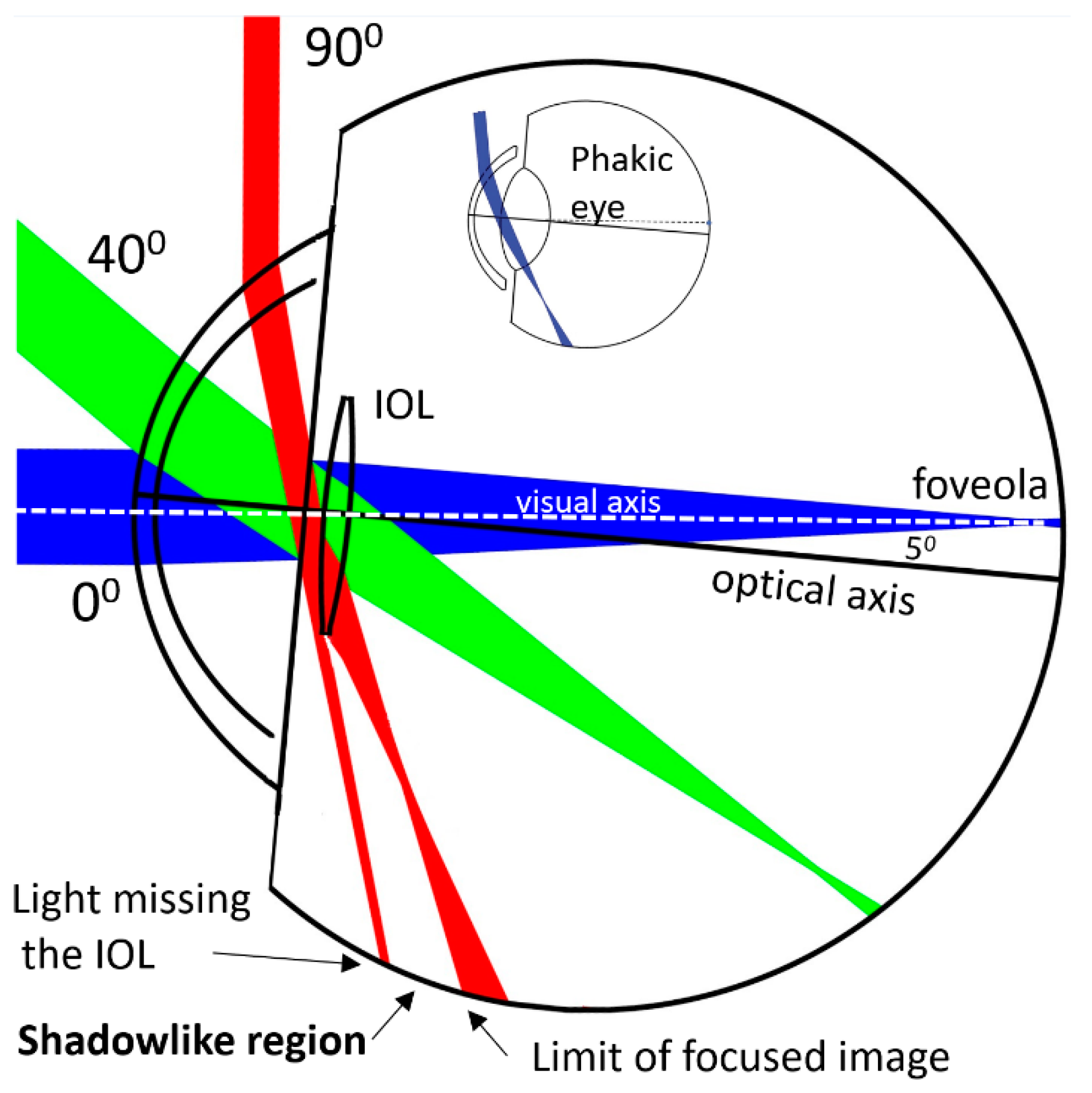
An evaluation of why a small number of patients with intraocular lenses (IOLs) see bothersome dark shadows in the far periphery (negative dysphotopsia) involved modeling the eye at very large visual angles [1,2,3,4]. During this work, it was found that the intersection angle of the chief ray with the retina was substantially the same as the input visual angle over a very large range when it was calculated relative to the optical axis from the second nodal point (NP2) [2,5]. This would be expected for small angles, but it was not clear why that would also be the case for angles as large as 70–90°, and that is evaluated here. This evaluation utilizes a pseudophakic eye that has an IOL, but the overall optical properties are broadly similar to a phakic eye.
IOLs are surgically implanted during cataract surgery to replace the natural crystalline lens, with about 3.5 million operations in the US every year, leading to their use in over 5% of the total population, though predominantly in people aged over 60. Figure 1 illustrates the reason for this new interest in scaling the retina in the far periphery, because light rays that enter the eye at very large visual angles no longer pass through the IOL, a characteristic that is called “vignetting” in a conventional optical system. The main image goes dark, and this is likely to be the underlying cause of the peripheral “dark shadows” that are reported by some IOL patients. Light might also bypass the IOL and illuminate the peripheral retina directly, and with small pupils there can be a gap between the two illuminated regions. This can cause a shadow-like region that goes away as the pupil opens up. This is consistent with clinical reports, but there is still no clear consensus about the cause [6,7,8,9]. The dark shadow evaluations indicate that the limit of the visual field may be reduced for the pseudophakic eye due to vignetting, which is very unexpected after 50 years of IOL usage with nobody mentioning it, though “far peripheral vision” seems to have never been explored in detail, even for the phakic eye [1].
To model the shadowlike effect, there is a need to match locations on the retina to the input visual angles that “appear” to correspond to them, because at very large angles a single input beam can bifurcate so that it illuminates two retinal locations (Figure 1). The limiting visual angle in the temporal direction for the phakic eye is generally thought to be 105°, though it is not routinely measured, and there are almost no clinical measurements for any eye for the region at angles of 90° and above [1]. Strasburger recently summarized the available literature [10]. Generally, nobody complains about this visual region, which may be why it is unexplored, but although resolution is poor in the far periphery, there is high sensitivity to motion, and it is part of the visual environment that we perceive all the time.
Methods for scaling the retina of a phakic eye that has a natural crystalline lens, rather than an IOL, have been discussed before [11,12]. The purpose of the earlier work seems to have primarily been to scale retinal features, and to help with activities such as estimating light intensity variations across the retina, rather than to specifically evaluate any value that the scaling might provide to vision itself. There are also other papers that discuss wide angle models for the eye [13], but with angles typically extending only to perhaps 40° (Figure 1), and with an emphasis on the quality of individual image points. With the visual system as a whole, there is perhaps always the thought that the brain can adjust the image scaling. However, linearity with respect to angle seems to be a characteristic of the optical properties of the eye, and the parameters that appear to be providing this benefit have been evaluated here using raytracing. Initially, the nodal point concept was explored to see if it was also useful somehow at large angles, but this led to an alternative representation using chief rays, which are more representative of image locations in the presence of aberrations.
2. Materials and Methods
An average pseudophakic model eye that has been described before [2] was evaluated using the Zemax raytrace software (Zemax, Kirkland, WA, USA). It had been found previously that phakic and pseudophakic eye models had broadly similar behavior, and retinal scaling for a phakic eye model had been used to evaluate a pseudophakic eye [2,3,14]. The model eye was also simplified to be rotationally symmetric by removing the decentration of the IOL and using the optical axis as the reference (which is typically rotated 5° from the visual axis (Figure 1)). The optical system is then more similar to a traditional textbook example for evaluating the nodal point, without the complications of a decentered gradient index crystalline lens, and it is also similar to eye models that are widely used. The model represents an average eye, with corneal radius of curvature values of 7.76 and 6.36 mm (index 1.376), corneal thickness of 0.55 mm, followed by a 3.45 mm aqueous depth to a thin iris, and then by 0.5 mm to the IOL. The IOL has equal spherical surfaces with radii of 19.69 mm, a center thickness of 0.66 mm, and a refractive index of 1.55 (power = 21 D). The axial length is 23.5 mm, and the retina is a sphere with a radius of 12 mm. The second nodal point (NP2) is given by Zemax to be at 7.03 mm relative to the anterior cornea.
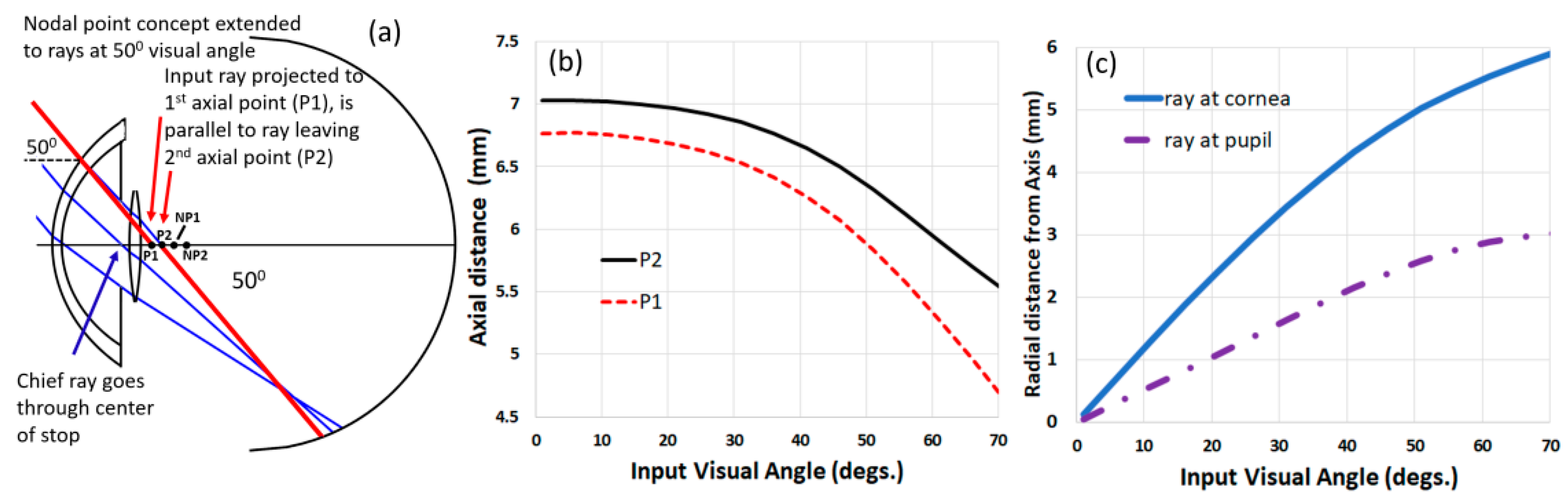
The nodal point is a paraxial property, with an input ray angle projected to the first nodal point (NP1) being parallel to the same ray in image space that is projected back to the second nodal point (NP2) (Figure 2a). The nodal point concept was extended to large angles here, with rays being evaluated in Zemax until a ray was found where input and output angles were parallel, for a large range of input visual angles. The rays were then extended to the optical axis to define points P1 and P2. The example of parallel rays in red in Figure 2a is for 50°, with the pupil diameter set to 5 mm, which just happens to also correspond to the marginal ray location (the last ray that is just transmitted by the pupil). The internal ray paths can also be seen here in blue, though these are usually not depicted when the nodal point situation is sketched in a textbook. It was found that as the input angle increased, the input ray moved laterally across the surface of the cornea, and that the axial points moved towards the anterior. The values were recorded and plotted.
A more useful ray was found to be the chief ray, passing through the center of the pupil, because this indicates the general direction of an imaging ray bundle even if the image is quite aberrated and defocused [15]. Chief rays were back projected from the retina to the optical axis to determine where the image rays appeared to come from (which for small angles is the location of the exit pupil, which is another paraxial parameter). The raytrace results led to a re-evaluation of publications relating to both cardinal points and the eye, and an Excel spreadsheet was then used to plot geometrical relationships. This led to a simplified equation that approximately described the angular rescaling from the exit pupil to both the nodal point and the center of the retinal sphere.
3. Results
3.1. Evaluating the Nodal Point Criterion over a Large Range of Angles
The axial intersections of parallel input and output rays are plotted in Figure 2b. These are the distances in mm from the anterior corneal apex, and for small input angles the axial ray locations match the traditional nodal point values, so that P1 = NP1, and P2 = NP2, with the curves in Figure 2b being flat to about 10 degrees of input visual angle. As the input angle increased, the points moved anteriorly, with the input ray also tracking across the surface of the cornea, and across the pupil plane (Figure 2c). The rays became increasingly peripheral and aberrated as the input angle increased, and for the example angle in Figure 2a, the ray would not even be transmitted by the pupil if it was any smaller. These results indicate that parallel input and output rays do not define unique axial points that can be used as reference points for angular measurements when angles are large.
3.2. Chief Ray Evaluation
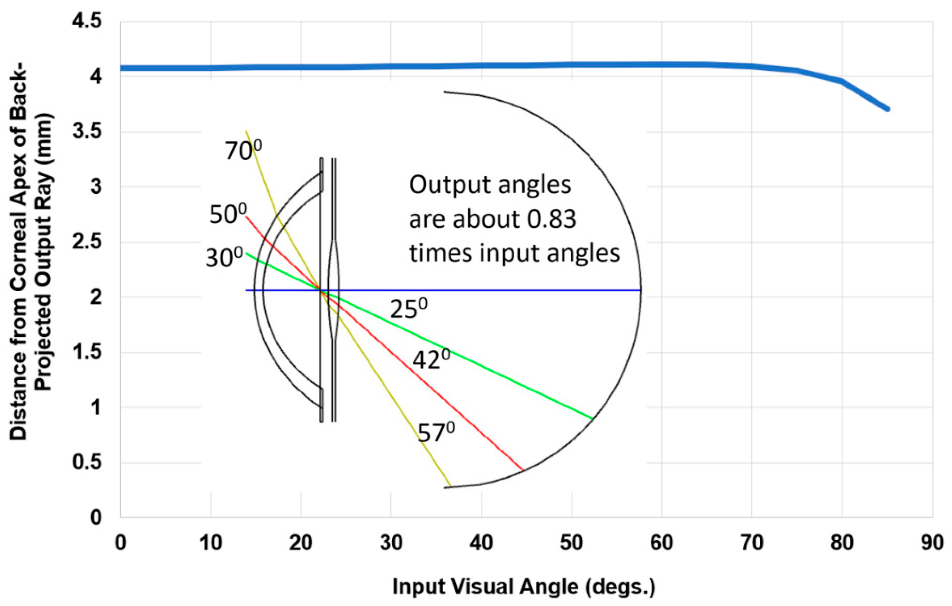
The chief rays that pass through the center of the pupil are more appropriate for explaining scaling, because they indicate the general direction of the imaging ray bundle, even if the image is aberrated and defocused. Figure 3 plots the axial location of where chief rays at the image appear to come from, by back projecting the rays from the retina to the optical axis. These are all very close to the stop itself, which is a thin iris in this model at 4 mm from the anterior corneal vertex. They are also approximately at the paraxial exit pupil of the eye, which is 4.08 mm inside the eye. In addition to these image rays primarily coming from the same point, the image angles were also approximately 0.83 times the input angle, and these are plotted as the lowest curve in Figure 4. It is the linearity of the angles at this point that is the basis for the overall angular linearity for the eye, with high linearity over 60–70° of input angle, and then a very modest droop at higher angles.
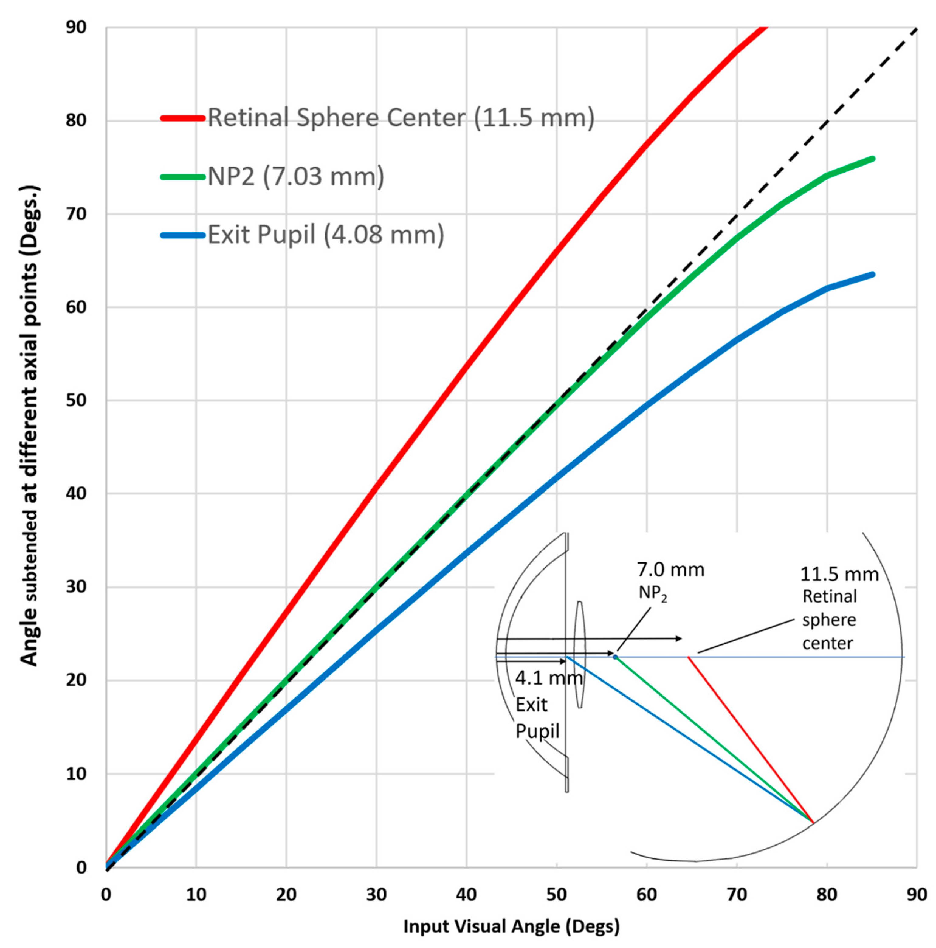
The second nodal point is of particular interest as a reference point because of its angular properties at small angles, and angles to chief ray intersections with the retina are also plotted in Figure 4 relative to NP2, along with angles relative to the center of the retinal sphere, which is also a special location. All three curves are highly linear for smaller angles, with angles at NP2 also having a slope that is approximately 1, so that the retinal angles approximately equal the input angles. This is not the same as the paraxial calculation that is used to define the nodal points when angles are small.
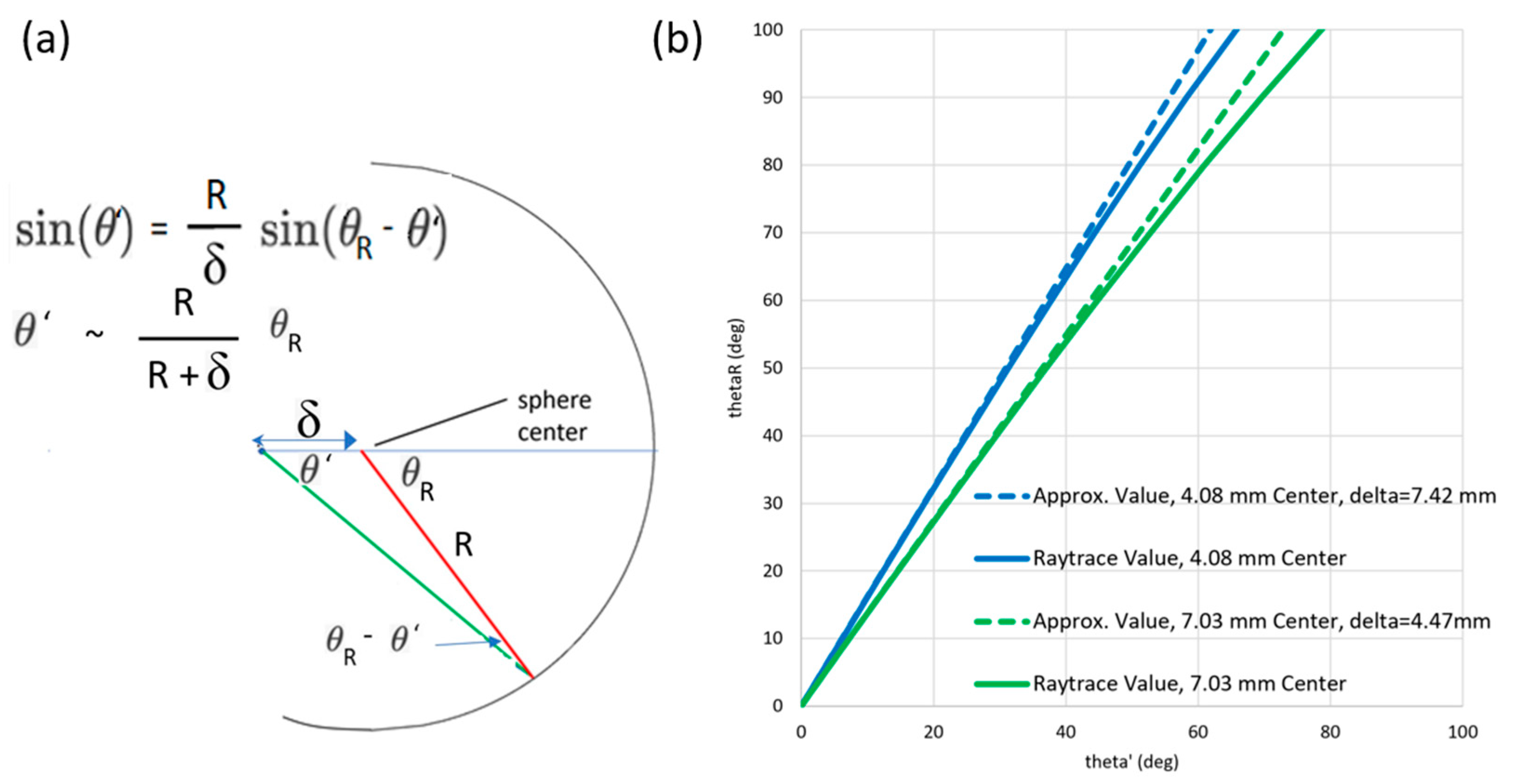
The underlying geometry that performs the rescaling between the reference points is illustrated in Figure 5a, using the center of the retinal sphere as the main reference. The retina is the surface that maintains the angular linearity relative to different axial points, by curving around to meet the rays, and intercepting them at earlier locations. At first glance Figure 5a resembles a familiar construction that involves triangles and circles, but the extra point is not very closely related to the circle, apart from being on a radial line. An exact equation using sines is given in Figure 5a, but this does not seem to simplify to a trivial equation that involves simple angles when large angles are used. An alternative simple approximation equation was found, which is unexpectedly the small angle approximation for the other equation, and this is also given in Figure 5a, with both relationships plotted in Figure 5b for the two delta values of interest. The simplified slope of R/(R + delta) is also the scale that would be achieved using sectors of a circle if delta was along the direction bisecting twice the angle (though the arc radii would also change as the angle varied). Slightly different linear fits could also be done to different lengths of the plots in Figure 5b.
4. Discussion
The raytrace calculations show that chief ray angles at the exit pupil are quite linearly related to input visual angles, and that the linearity is maintained for other axial reference points because the retina curves around to meet the rays as the angle increases. When angles are calculated relative to the nodal point, they are approximately the same as input visual angles, and it is possible that the phrase “nodal point” may sometimes be used to designate a geometrical reference point for the eye, rather than it being used to describe the paraxial optical properties. The calculations here confirm that this is a good choice for a reference point, but they also confirm that the “nodal point” concept itself is only valid for relatively small angles. Using the term for this broader purpose is somewhat misleading.
One example in the literature of the use of the nodal point as a reference at large angles is the scaling of the retina in monkey and human MRI images [16,17,18], where for a phakic eye it is assumed that NP2 is at the posterior pole of the crystalline lens. This is a location that actually has a physical characteristic, unlike the nodal point location, which would need to be calculated, yet it is close, and the posterior pole itself is designated NP2. This seems to be an excellent pragmatic choice, and then angles measured to that point are approximately the same as input visual angles, though it is not clear where this insight originated.
Angular scaling is also depicted implicitly in the patent literature relating to lenses designed for indirect ophthalmoscopy [19], with imaging in the reverse direction. Rays from retinal points appear to have similar angular linearity in the region of the pupil, and this region is then projected out of the eye with angular control to form an image that can be viewed in front of the eye.
A parameter that is related to this discussion is the “paraxial pupil ray angle ratio”, which was calculated by Atchison et al. to be about 0.82 for a phakic eye using small paraxial angles [15]. This is the angle subtended at the exit pupil divided by the input angle. That value was for one particular schematic phakic eye, and its magnitude is similar to the value of 0.83 that was found here using raytracing at the exit pupil for a pseudophakic eye, with the angular relationship holding to very large angles (Figure 4).
Some earlier methods to scale the retina also used chief rays and the angle at the exit pupil, but it is possible that the angles themselves were not specifically calculated because they were not relevant at the time [11,12]. The scale factor of 1.33 here can be used to approximately rescale input angles to angles subtended at the center of the retinal sphere, and the distance along the retina can then be calculated using the equation for an arc, with distances for this pseudophakic eye broadly similar to those in Suheimat et al. for a phakic eye [12]. This indicates a consistency with earlier calculations, but with a new approach where the calculation is divided into two separate parts, with an emphasis on angles rather than distances along the retina.
The basis for the angular linearity of the eye actually comes from the cornea and lens, rather than the paraxial nodal point criterion, with the initial raytracing of chief rays to the exit pupil rescaling the angles by approximately a constant value of 0.83 over a very large angular range for this particular average pseudophakic eye. This is not something that can be seen in a simple sketch of the eye. With that linearity established, a second method comes into play to maintain the linearity, with the curvature of the retina compensating for increasing angle. Curved image surfaces are rarely encountered, with most detectors used for lens design being flat, and even though Zemax is used here for raytracing, the software itself envisages that the image will be projected down onto a plane that passes through the apex of the curved image surface for analysis (though some other calculations are projected onto local tangent planes). Perhaps this concept originated with fiberoptic faceplates, but it leads to a need for caution when Zemax is used for widefield imaging of the eye. The Zemax calculations here are only for chief rays, with other evaluations being performed in Excel.
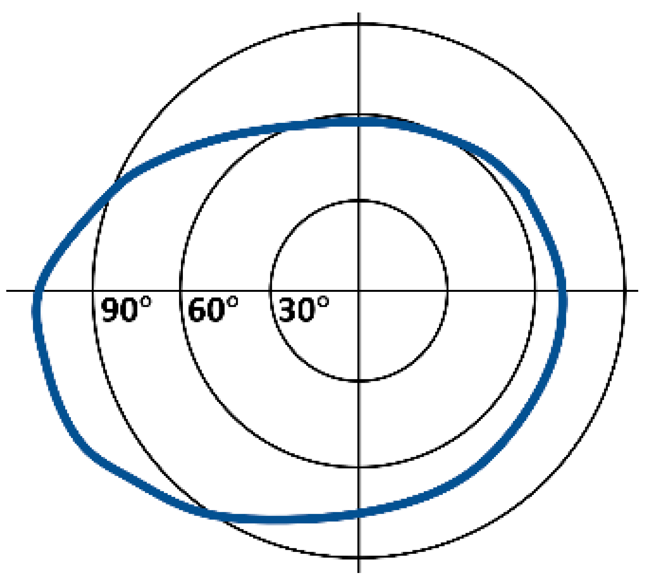
It is not clear if there is a field of study yet that relates the measurement of visual angles outside the eye to the measurement of corresponding retinal image regions, which might be done using trans-scleral illumination somehow [1]. This may be useful for an improved understanding of topics such as negative dysphotopsia. The approximate angular properties can be summarized using the type of polar plot that is used to record perimetry data (Figure 6). Perimetry is the main clinical test for large visual angles, but normally the pupil diameter is neither controlled nor measured, angles only go up to 90°, and there is no record for where a stimulus is seen (which are all concerns when evaluating negative dysphotopsia [3]). The isopter curve sketched in Figure 6 is similar to ones created for young phakic eyes, using a special perimeter where the fixation target can be moved in order to make measurements beyond the normal 90° limit [20]. The figure legend indicates how although this type of plot is only normally used to represent visual angles, for the region with linear scaling, it can also represent angles and distances within the eye. Linearity is very high up to 70° of visual angle, which is about the angle at which the image is formed on the side of the eye (the equator), with the retina oriented towards the posterior for larger angles. There is increasing non-linearity in the relationship at very large angles, though this is still modest.
There are various limitations to the evaluation here, including the use of a single symmetrical eye, and a 12 mm spherical retinal surface. However, these are common simplifications, and they allow the main trends to be identified. The angles also do not include a 5° offset to the foveola [1,2] (though that would tend to increase the linear range). Chief rays are used for the main evaluation, and the imaging system has a lot of aberrations at large angles. Even defocus is not taken into account, and a conventional imaging evaluation would probably use field curvature to describe defocus, with the linearity of the retinal angles being related to distortion. The model also uses a thin iris, though the actual iris has a thickness that can affect rays at very large angles [21]. The evaluation is also for a pseudophakic eye, without equivalent calculations here for a phakic eye (though modeling elsewhere indicates that imaging properties are similar [12], and also that modeling the crystalline lens at very large angles is challenging [3]). There may also be scaling changes between the phakic and pseudophakic eye that may affect the perception of image locations. Despite these limitations, however, the analysis describes how radial retinal image locations are generally linearly related to input visual angle over a very large range, and that this does not depend on the paraxial definition of the nodal point.
The original stimulus for this work was to evaluate peripheral dark shadows, which led to the finding that the “far peripheral vision” region beyond 60° is rarely measured or modeled. That led to the topic of linearity across the entire range of visual angles, and although the linearity seems to be generally recognized, discussions are not always clear. The visual system probably takes advantage of the linear retinal scaling [22,23], and a recent summary that includes vision in the far periphery is given by Strasburger [10]. In addition to linearity, the nodal point location does appear to provide scaling that matches the input angle directly, but that is not because of the paraxial nodal point characteristics of the lens system, but is due instead to other characteristics of the eye, involving the cornea, the lens, and the retinal curvature.
Funding
This research received no external funding.
Institutional Review Board Statement
Not applicable.
Acknowledgments
Grateful thanks to Hans Strasburger for email discussions, and to anonymous reviewers of an earlier draft.
Conflicts of Interest
The author declares no conflict of interest.
Conference Presentation
Part of this work was presented at the Optical Society of America Annual Meeting, Frontiers in Optics, Online, September 2020.
References
- Simpson, M.J. Mini-review: Far peripheral vision. Vis. Res. 2017, 140, 96–104. [Google Scholar] [CrossRef]
- Holladay, J.T.; Simpson, M.J. Negative dysphotopsia: Causes and rationale for prevention and treatment. J. Cataract Refract. Surg. 2017, 43, 263–275. [Google Scholar] [CrossRef]
- Simpson, M.J. Intraocular lens far peripheral vision: Image detail and negative dysphotopsia. J. Cataract Refract. Surg. 2020, 46, 451–458. [Google Scholar] [CrossRef] [PubMed]
- Simpson, M.J. Comment on: Distinct differences in anterior chamber configuration and peripheral aberrations in negative dysphotopsia. J. Cataract Refract. Surg. 2021, 47, 139–140. [Google Scholar] [CrossRef] [PubMed]
- Simpson, M.J. Scaling the Retinal Image of the Pseudophakic Eye Using the Nodal Point. In Frontiers in Optics/Laser Science; Lee, B., Mazzali, C., Corwin, K., Jones, R.J., Eds.; OSA Technical Digest (Optical Society of America): Washington, DC, USA, 2020. [Google Scholar]
- Masket, S.; Fram, N.R. Pseudophakic Dysphotopsia: A Review of Incidence, Etiology and Treatment of Positive and Negative Dysphotopsia. Ophthalmology 2020. [Google Scholar] [CrossRef]
- Wenzel, M.; Langenbucher, A.; Eppig, T. Causes, Diagnosis and Therapy of Negative Dysphotopsia. Klin. Monbl. Augenheilkd. 2019, 767–776. [Google Scholar] [CrossRef] [Green Version]
- Van Vught, L.; Luyten, G.P.M.; Beenakker, J.-W.M. Distinct differences in anterior chamber configuration and peripheral aberrations in negative dysphotopsia. J. Cataract Refract. Surg. 2020, 46, 1007–1015. [Google Scholar] [CrossRef] [PubMed]
- Makhotkina, N.Y.; Berendschot, T.T.J.M.; Nuijts, R.M.M.A. Objective evaluation of negative dysphotopsia with Goldmann kinetic perimetry. J. Cataract Refract. Surg. 2016, 42, 1626–1633. [Google Scholar] [CrossRef] [PubMed]
- Strasburger, H. Seven Myths on Crowding and Peripheral Vision. Iperception 2020, 11, 1–46. [Google Scholar]
- Drasdo, N.; Fowler, C.W. Non-linear projection of the retinal image in a wide-angle schematic eye. Br. J. Ophthalmol. 1974, 58, 709–714. [Google Scholar] [CrossRef] [PubMed] [Green Version]
- Suheimat, M.; Zhu, H.; Lambert, A.; Atchison, D.A. Relationship between retinal distance and object field angles for finite schematic eyes. Ophthalmic Physiol. Opt. 2016, 36, 404–410. [Google Scholar] [CrossRef] [PubMed] [Green Version]
- Escudero-Sanz, I.; Navarro, R. Off-axis aberrations of a wide-angle schematic eye model. J. Opt. Soc. Am. A 1999, 16, 1881. [Google Scholar] [CrossRef] [PubMed] [Green Version]
- Simpson, M.J. Simulated images of intraocular lens negative dysphotopsia and visual phenomena. J. Opt. Soc. Am. A Opt. Image Sci. Vis. 2019, 36, B44–B51. [Google Scholar] [CrossRef] [PubMed]
- Atchison, D.A.; Smith, G. Optics of the Human Eye; Butterworth-Heinemann: Oxford, UK, 2002. [Google Scholar]
- Gilmartin, B.; Nagra, M.; Logan, N.S. Shape of the posterior vitreous chamber in human emmetropia and myopia. Investig. Ophthalmol. Vis. Sci. 2013, 54, 7240–7251. [Google Scholar] [CrossRef] [PubMed] [Green Version]
- Smith, E.L.; Hung, L.F.; Huang, J.; Blasdel, T.L.; Humbird, T.L.; Bockhorst, K.H. Effects of optical defocus on refractive development in monkeys: Evidence for local, regionally selective mechanisms. Investig. Ophthalmol. Vis. Sci. 2010, 51, 3864–3873. [Google Scholar] [CrossRef] [PubMed]
- Huang, J.; Hung, L.-F.; Ramamirtham, R.; Blasdel, T.L.; Humbird, T.L.; Bockhorst, K.H.; Smith, E.L. Effects of form deprivation on peripheral refractions and ocular shape in infant rhesus monkeys (Macaca mulatta). Investig. Ophthalmol. Vis. Sci. 2009, 50, 4033–4044. [Google Scholar] [CrossRef] [PubMed] [Green Version]
- Volk, D.A. Indirect Ophthalmoscopy Contact Lens Device with Compound Contact Lens Element. U.S. Patent 5,523,810, 4 June 1996. [Google Scholar]
- Bain, C.; Marín-Franch, I.; McNaught, I.A.; Artes, P. The limits of the far peripheral visual field. Investig. Ophthalmol. Vis. Sci. 2018, 59, 1272. [Google Scholar]
- Simpson, M.J.; Muzyka-Woźniak, M. Iris characteristics affecting far peripheral vision and negative dysphotopsia. J. Cataract Refract. Surg. 2018, 44, 459–465. [Google Scholar] [CrossRef]
- Strasburger, H. On the cortical mapping function–visual space, cortical space, and crowding. bioRxiv 2019. [Google Scholar] [CrossRef] [Green Version]
- Strasburger, H.; Jüttner, M. Peripheral vision and pattern recognition: A review. J. Vis. 2015, 11, 1–82. [Google Scholar] [CrossRef] [PubMed] [Green Version]
Figure 1.
Raytrace plot for a pseudophakic right eye from above, with 2.5 mm actual pupil diameter. At large angles there is vignetting at the intraocular lens (IOL) and the main image goes dark. Light can also bypass the IOL and illuminate the retina directly, though that light comes from a lower visual angle than for the phakic eye.

Figure 2.
The nodal point concept extended to large angles. (a) Zemax drawing. (b) Axial distance from corneal apex of points with identical input and output angles as visual angle increases (P1 and P2). (c) Radial distance from axis at cornea and pupil for points in (b).
Figure 2.
The nodal point concept extended to large angles. (a) Zemax drawing. (b) Axial distance from corneal apex of points with identical input and output angles as visual angle increases (P1 and P2). (c) Radial distance from axis at cornea and pupil for points in (b).

Figure 3.
For a large range of input angles, output angles for chief rays come from approximately the axial exit pupil location, with angles that are about 0.83 times the input angles.
Figure 3.
For a large range of input angles, output angles for chief rays come from approximately the axial exit pupil location, with angles that are about 0.83 times the input angles.

Figure 4.
Angles to chief ray intersections with the retina calculated from the exit pupil, the second nodal point NP2, and the center of retinal sphere. Angles at NP2 are approximately equal to input angles over a very large range. Angles at the retinal sphere center can be converted to linear distances along the retina using the arc calculation (distance = radius * angle in radians).

Figure 5.
(a) The geometrical relationship that rescales angles by approximately a constant over a large angular range. (b) Plots for the exact and approximate values. As the angle increases, the curve of the retina adjusts the intersection point, which maintains linearity.
Figure 5.
(a) The geometrical relationship that rescales angles by approximately a constant over a large angular range. (b) Plots for the exact and approximate values. As the angle increases, the curve of the retina adjusts the intersection point, which maintains linearity.

Figure 6.
An isopter plot of visual thresholds for external targets. This might also represent internal angles at NP2, angles at the exit pupil (scaled by 1/0.83), or angles at the retinal center (scaled by 1/1.33) (and also distances along the retina if converted to arc lengths). A possible limiting isopter for a young phakic eye is sketched, exceeding the normal 90° limit of a perimeter [20].

Publisher’s Note: MDPI stays neutral with regard to jurisdictional claims in published maps and institutional affiliations. |
© 2021 by the author. Licensee MDPI, Basel, Switzerland. This article is an open access article distributed under the terms and conditions of the Creative Commons Attribution (CC BY) license (https://creativecommons.org/licenses/by/4.0/).
Share and Cite
MDPI and ACS Style
Simpson, M.J. Scaling the Retinal Image of the Wide-Angle Eye Using the Nodal Point. Photonics 2021, 8, 284. https://0-doi-org.brum.beds.ac.uk/10.3390/photonics8070284
AMA Style
Simpson MJ. Scaling the Retinal Image of the Wide-Angle Eye Using the Nodal Point. Photonics. 2021; 8(7):284. https://0-doi-org.brum.beds.ac.uk/10.3390/photonics8070284
Chicago/Turabian StyleSimpson, Michael J. 2021. "Scaling the Retinal Image of the Wide-Angle Eye Using the Nodal Point" Photonics 8, no. 7: 284. https://0-doi-org.brum.beds.ac.uk/10.3390/photonics8070284
Note that from the first issue of 2016, this journal uses article numbers instead of page numbers. See further details here.