An Analysis of the Italian Lockdown in Retrospective Using Particle Swarm Optimization in Machine Learning Applied to an Epidemiological Model


1
IMT School for Advanced Studies Lucca, Piazza San Francesco 19, 55100 Lucca, Italy
2
TREE-TOWER s.r.l., Via della Chiesa XXXII trav. I n. 231, 55100 Lucca, Italy
Physics 2020, 2(3), 368-382; https://0-doi-org.brum.beds.ac.uk/10.3390/physics2030020
Submission received: 2 July 2020
/
Revised: 27 July 2020
/
Accepted: 29 July 2020
/
Published: 1 August 2020
(This article belongs to the Special Issue Physics Methods in Coronavirus Pandemic Analysis)
Abstract
:A critical analysis of the open data provided by the Italian Civil Protection Centre during phase 1 of Covid-19 epidemic—the so-called Italian lockdown—is herein proposed in relation to four of the most affected Italian regions, namely Lombardy, Reggio Emilia, Valle d’Aosta, and Veneto. A possible bias in the data induced by the extent in the use of medical swabs is found in relation to Valle d’Aosta and Veneto. Observed data are then interpreted using a Susceptible-Infectious-Recovered (SIR) epidemiological model enhanced with asymptomatic (infected and recovered) compartments, including lockdown effects through time-dependent model parameters. The initial number of susceptible individuals for each region is also considered as a parameter to be identified. The issue of parameters identification is herein addressed by a robust machine learning approach based on particle swarm optimization. Model predictions provide relevant information for policymakers in terms of the effect of lockdown measures in the different regions. The number of susceptible individuals involved in the epidemic, important for a safe release of lockdown during the next phases, is predicted to be around 10% of the population for Lombardy, 16% for Reggio Emilia, 18% for Veneto, and 40% for Valle d’Aosta.
1. Introduction
To contrast the spread of the severe acute respiratory syndrome coronavirus 2 (SARS-CoV-2), called Covid-19 in the sequel for the sake of brevity, different healthcare policies and lockdown measures have been put into practice worldwide [1,2]. Just to mention a few relevant instances, extreme isolation measures were taken in the Hubei region in China, the epicenter of the Covid-19 pandemic [3], to rapidly reduce the spread of new infections. Tracking the movement of infected people and their contacts using smartphones was firstly implemented in South Korea as a possible remedy to extreme social distancing.
Lockdown measures with increasing severity over time were adopted in Italy, motivated by the urgent need to flatten the peak of individuals requiring intensive healthcare treatment, due to the risk of suffering from a lack of intensive units in hospitals. This led to a sequence of progressive lockdowns. Initially, a “red zone” (quarantine zone) was set just for the municipalities of the province of Lodi in the region of Lombardy. This was followed by an extension of the red zone up to the whole country, giving rise to the so-called “Italian lockdown”, from March 10 up to the end of April 2020. Reduction of the severity of social distancing took place in various regions in correspondence of the first long weekend of May (from the 1st of May, public holiday, till the 3rd of May), and on May 4 the so-called phase 2 started. The impact of mobility restrictions upon Covid-19 epidemic spread was significant [4].
Uncertainties in forecasting the evolution of the epidemic arose, with official predictions by the Italian Government initially included in a draft decree circulated the day before March 8, and then removed from the finalized version. In retrospect, such tentative forecasts were underestimating the actual spread of the contagion. The majority of them were based on analogies between Italy and Hubei, supported by the similar population size. While this approach was justified at the beginning of epidemic, where an exponential trend was mainly governed by the basic reproduction number [5], its further use for longer forecasts was questionable for a series of reasons, including the fact that the emergent dynamics depended upon the lockdown measures taken over time, the severity of social distancing was different in Italy and in Hubei, and fitting and extrapolations done on each single compartment of individuals (infectious, recovered, dead) separately from the others did not include the underlying nonlinear relations between them.
The application of Susceptible-Infectious-Recovered (SIR) epidemiological models [1,6,7] would offer some advantages, but their application to interpret observed data is not as straightforward. SIR models should be applied at a small scale (province or region) due to the large inhomogeneity of epidemic spread across Italy, and due to the different lockdown measures adopted in each region. Their applicability to regions where few cases were noticed might require the incorporation of stochastic effects [8]. Moreover, the large number of asymptomatic individuals requires considering also such a compartment [9,10,11], for which there is no accurate data available. Moreover, observed data collected by the Italian Civil Protection Centre on a daily basis [12] may also present some criticalities, including the effect of the number of medical swabs upon the reported cases of symptomatic infected people.
Therefore, even for relatively simple SIR models to be used to interpret observed regional trends, the number of model parameters rapidly increases, and their robust identification is an open issue. As a possible remedy to manual identification, which would be too complex and might inevitably lead to a lack of scientific rigor in the comparison of model predictions, a machine learning approach, used to test the reliability of SIR model forecasts in [13], could be employed.
The present study retrospectively examines the phase 1 for four Italian regions strongly affected by Covid-19 epidemic, namely Lombardy, Emilia Romagna, Valle d’Aosta, and Veneto. In spite of all being located in northern Italy, they have different population size, and experienced different lockdown measures over time, had different healthcare policies, and also experienced different extents in the use of medical swabs for Covid-19 testing. Modeling the effect of lockdown measures and epidemic dynamics is relevant for comparing the effect of different policies worldwide (see for example, recent studies for Greece [14] and Germany [15,16]).
In Section 2.1, a critical analysis of the data provided by the Civil Protection Centre is made, examining the uncertainties and the possible bias caused by the differences in the extent of the use of medical swabs. In Section 2.2 and Section 2.3, methods are presented, which consist of an SIR epidemiological model accounting for living dynamics, asymptomatic individuals and the effect of lockdown measures. The machine learning approach based on particle swarm optimization (PSO) is detailed in the same section, explaining its application to the Covid-19 scenario with up to seven parameters identified. Section 3 reports the main results of the simulations; a critical comparison allows assessing the impact of lockdown in such regions. Section 4 concludes the article with recommendations for policymakers. Particularly relevant is the estimated number of the initial susceptible individuals, which varied from region to region, and its knowledge is an important indicator for a safe implementation of released lockdown measures in the next phases, and assess the risk of further outbreaks.
2. Data and Methods
2.1. Critical Analysis of Epidemiological Data at the Regional Level
The Italian regions of Lombardy, Emilia Romagna, Valle d’Aosta, and Veneto have been herein selected since they were among the regions with the largest spread of the contagion. Moreover, they experienced different lockdown measures over time, had different healthcare policies, different initial dates of outbreaks, and are also characterized by different population sizes. Data from the beginning of Covid-19 epidemic in Italy (day 1 corresponds to the 24th of February 2020) till the 30th of April 2020 (last day of phase 1, the so-called Italian lockdown) were considered. Those data are publicly available on the portal of the Italian Civil Protection Centre [12].
Lombardy has a population size of about 10.4 million inhabitants and was the epicenter of the first major outbreak in Italy. The first lockdown began around the 21st of February 2020, covering eleven municipalities of the province of Lodi that were included in the so-called “red zone” (quarantine zone). On the 8th of March, Italian Prime Minister Conte announced the expansion of the quarantine zone to cover much of northern Italy. With that decree, the initial “red zone” was also abolished, though the municipalities were still within the quarantined area. The locked down area, as of 8 March, covered the entirety of the region of Lombardy, in addition to 14 provinces in Piemonte, Veneto, Emilia-Romagna, and Marche. On the evening of 9 March, the quarantine measures were expanded to the entire country, coming into effect the next day. Conte announced on 11 March that the lockdown would be tightened, with all commercial and retail businesses, except those providing essential services, like grocery stores, food stores, and pharmacies, closed down. Such lockdown measures were prolongated till 4 May. Hence, Lombardy was subject to all the above lockdown measures of increasing intensity.
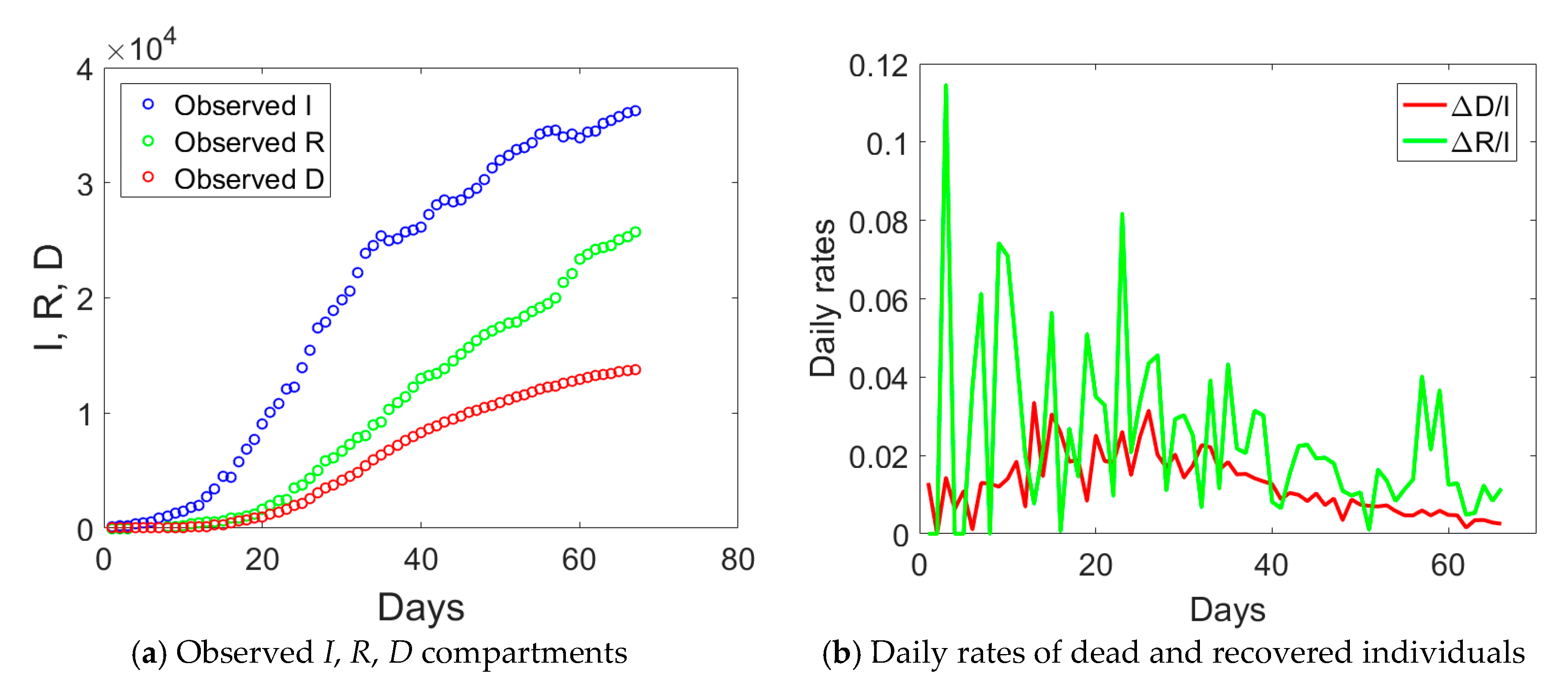
The observed data for the I (actual infected), R (recovered), and D (dead individuals) compartments for Lombardy are shown in Figure 1a. The curve corresponding to actual infected individuals (blue circles) had an initial exponential growth, subsequently slowed down after day no. 18, 21 days after the implementation of the first lockdown to the province of Lodi. Another change of slope occurred at day no. 34, again 21 days from the second lockdown that was extending the red zone to the whole Lombardy. At the end of phase 1, the peak of actual infectious individuals was not yet reached. Daily rates ΔD/I and ΔR/I (Δ stays for the difference between compartmental values over two consecutive days) computed from Figure 1a are plotted in Figure 1b and show some distinct trends: an initial increasing one till day no. 18, a plateau, and then a progressive decay over time.
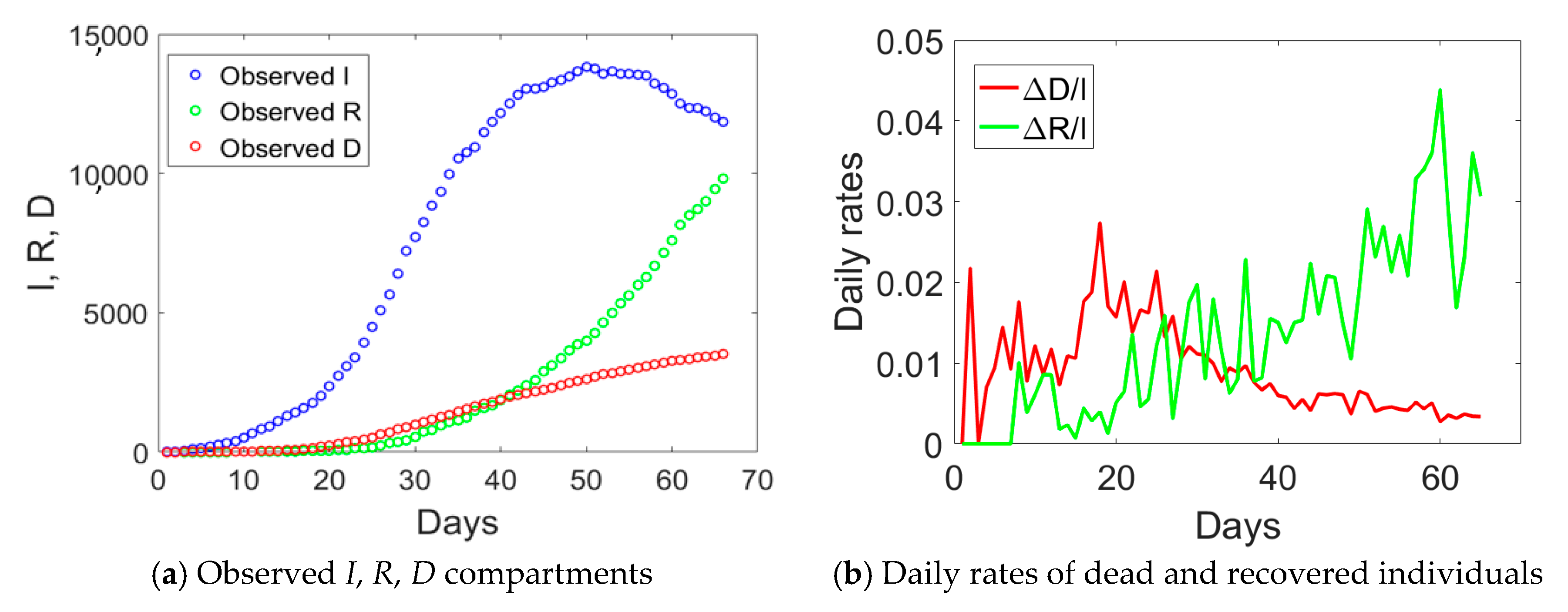
Emilia Romagna has a population size of 4.459 million inhabitants and saw the provinces of Modena, Parma, Piacenza, and Reggio Emilia included in the red zone on the 8th of March. Such an intermediate measure was very short in time, since it was followed by the Italian lockdown on the 9th of March. If we examine the observed I, R, and D data for Emilia Romagna in Figure 2a, one notices an evident change of curvature at day no. 34, about 21 days from the day when lockdown measures took place. The curve corresponding to the actual infected individuals (blue circles) reached the peak at day no. 50. Daily rates ΔD/I and ΔR/I computed from Figure 2a are plotted in Figure 2b. The daily rate of deaths, ΔD/I, had an initial increasing trend followed by a decay over time, similarly to Lombardy. The absence of a plateau could be probably related to the fact that Emilia Romagna was subject to two lockdown measures with just one day of time lag between them, rather than 16 days as in Lombardy. The daily rate of recovered individuals shows an increasing trend over time, opposite to the situation observed in Lombardy.
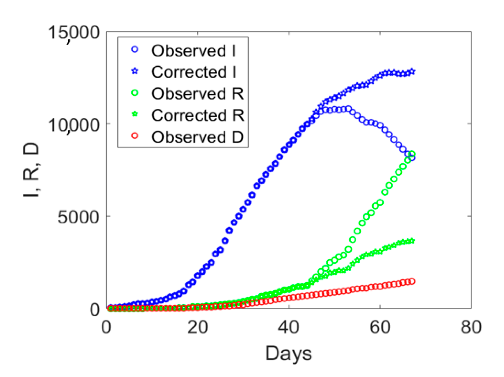
Valle d’Aosta is the smallest Italian region with only 125,666 inhabitants. It was subject to the Italian lockdown taking place on the 9th of March and experienced the largest number of Covid-19 deaths per population.
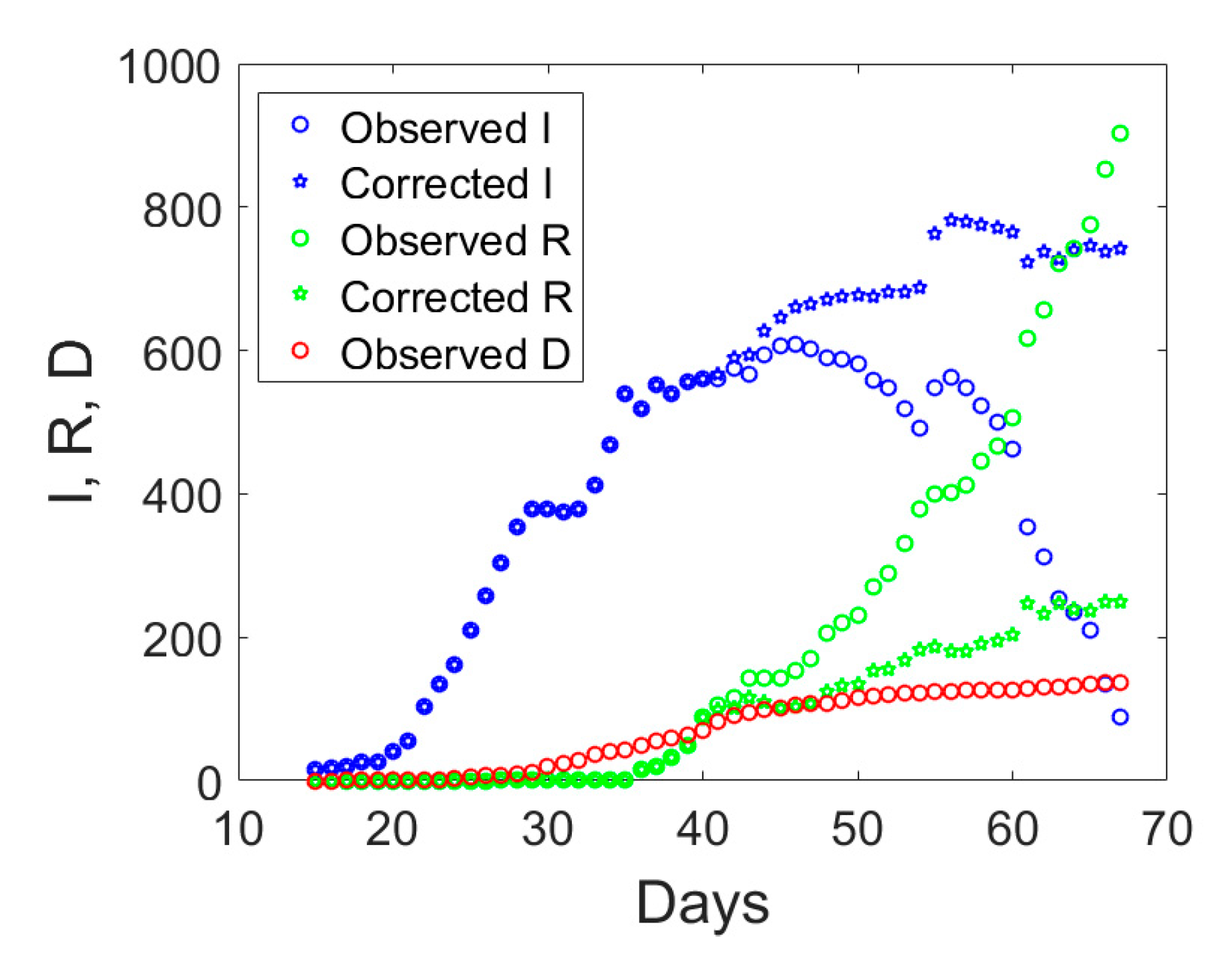
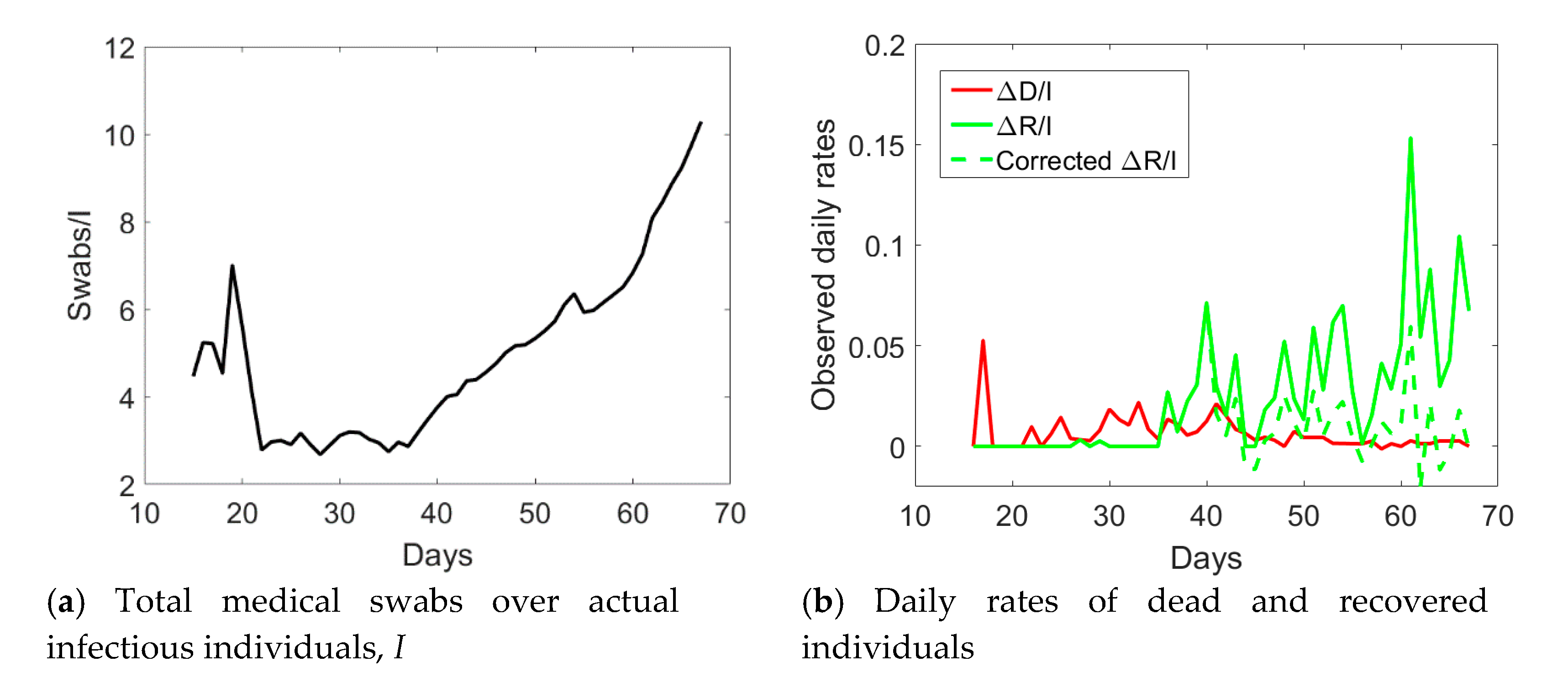
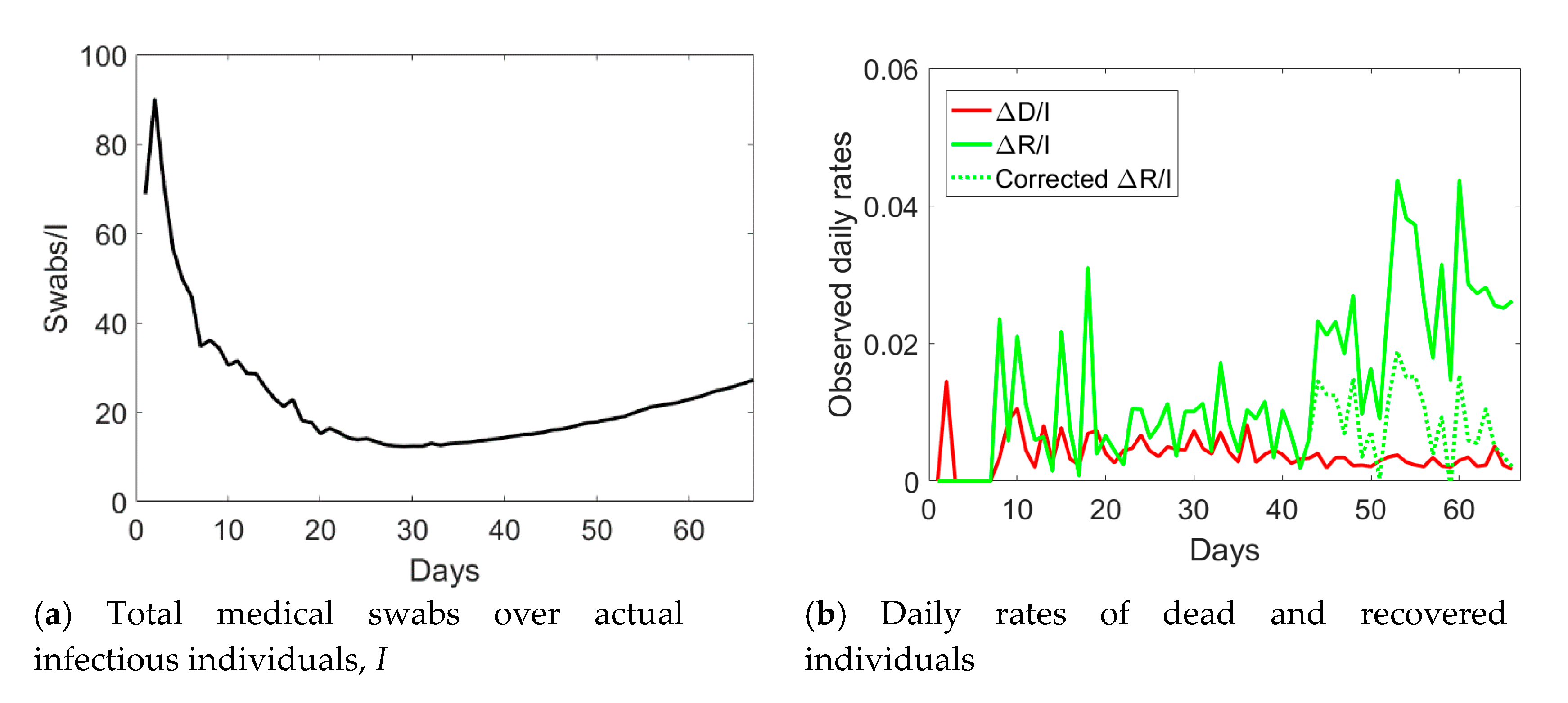
If we examine the observed I, R, and D data displayed with circles in Figure 3, one notices an abrupt sudden increase in recovered individuals after day no. 40. The time series of the actual infected individuals presented also sudden jumps at days no. 40 and 55. To understand the possible reason for such a lack of smoothness in the observed data, one could examine the ratio between the cumulative number of medical swabs and the actual number of infectious individuals, Sw/I (see Figure 4a). Such a ratio was almost constant and reached a minimum at day no. 40. Afterwards, it linearly increased over time with a discontinuity at day no. 55. One could reasonably assume that when the quantity Sw/I was at the minimum at the early stage of the epidemic, swab tests were in a number almost strictly necessary to identify infected people claiming Covid-19 symptoms. Later, the increase in the use of medical swabs also to randomly test the population was likely leading to the identification of not only symptomatic, but also asymptomatic infected individuals. Since the open data in the compartment I include all the confirmed positive cases to Covid-19, regardless of their symptoms, one could expect that the observed data might be biased by the number of medical swabs. Overall, the number of asymptomatic cases is expected to increase as long as medical swabs are used to massively test the population even in absence of reported Covid-19 symptoms. This bias could affect the number of recovered individuals as well, which inevitably sums up the number of symptomatic and asymptomatic recovered patients, which could explain the sudden increase in the daily rate ΔR/I after day no. 40.
As a possible empirical correction to the observed data to retain only symptomatic cases in the I compartment, one could multiply the number of recovered individuals by the ratio between the number of medical swabs divided by the number of medical swabs at day no. 40, when Sw/I was minimum in the time series. Since this ratio is less than unity, the corrected number of recovered individuals will diminish as compared to the reported one. The actual number of asymptomatic infected individuals, I, will be computed as the total number of reported cases minus the number of deaths and the corrected number of recovered individuals. Hence, the actual number of symptomatic infected individuals would increase as compared to the observed data which include also some asymptomatic ones. The application of this correction to the data of Valle d’Aosta leads to the corrected time series shown in Figure 3 with pentagrams. The daily rate of the corrected recovered individuals shown in Figure 4b with a dashed green line is now oscillating around a constant average value, without the anomalous fast increasing trend (solid green line) observed from the reported observations.
Veneto has a population size of 4.9 million inhabitants. The provinces of Padua, Treviso, and Venice were subject to the lockdown on the 8th of March, followed by the Italian lockdown the day after. As compared to Lombardy, where hospitalization was the major healthcare solution, Veneto largely implemented home treatment. Moreover, Veneto was the only region able to purchase laboratory equipment for automatic testing of up to 9000 medical swabs per day. Such an infrastructure was announced to be operative since the 7th of April 2020, which corresponds to day no. 44 of the time series.
The augmented testing capabilities resulted in an increased number of observed recovered individuals and a fast decay of actual infected people after day no. 44 (see Figure 5). Correspondingly, the ratio Sw/I increased from its minimum value (see Figure 6a). The application of the correction to the data of Veneto, as previously done for Valle d’Aosta, but considering the number of medical swabs at day no. 44 as a reference, led to the corrected data shown with pentagrams in Figure 5. Such an empirical correction to the actual infected individuals to remove the asymptomatic ones is noteworthy, since the corrected time series shows that the peak was not yet reached in this region before the start of phase 2.
The corrected daily rate of recovered individuals is shown in Figure 6b with a green dashed line. As for Valle d’Aosta, the correction leads to a steady rate over time, rather than the anomalous growth reported (green solid line). The rate of dead individuals decreased over time after day no. 34, in line with the trend reported for the other regions.
2.2. An Epidemiological Model for Covid-19 Including Asymptomatic and Lockdown Effects to Interpret Observed Data
SIR epidemiological models have been the subject of intensive research which led to several variants to the basic model including only three compartments. Here, we refer to the model proposed elsewhere [11] to deal with the large number of asymptomatic individuals for Covid-19 epidemic in Italy. This includes two additional compartments representing asymptomatic infected (A) and unregistered recovered (U) individuals (i.e., the recovered asymptomatic patients). In the model, permanent immunity of individuals who were infected and recovered is postulated, which is realistic enough since few cases of repeated infections were reported during phase 1. Moreover, the compartment of dead individuals is also herein included to model living dynamics. As another major variant from the original model [11], for its application at the regional level, the population size (N) is split into two parts: one of initial susceptible individuals (N0), that are involved into the epidemic dynamics, and the other, of numerosity (N − N0), composed of people excluded from the Covid-19 epidemic thanks to the effect of the lockdown measures. This is motivated by the fact that many categories, such as public servants, started smart working from the emanation of the earliest lockdown measures, significantly reducing the probability of becoming susceptible to contagion.
Susceptible individuals S, who reduced their mobility but still had contacts justified by their urgent job activities, can evolve in one of the two classes of infected and infective people: symptomatic, which should match the corrected value I of reported infected people, and asymptomatic A. People can move from the compartment of symptomatic individuals into two other compartments, one of registered recovered, which should match the observed R data, and another of dead individuals, that should match the observed D data. People in the compartment of asymptomatic individuals, on the other hand, can be removed and pass to the compartment of unregistered recovered, U, which collects individuals passing unnoticed through the infection.
In formulae, the dynamics is described by the following set of nonlinearly coupled ordinary differential equations (ODEs):
Model parameters entering Equations (1)–(6) are represented by the coefficients β, γ, μ, η, and ξ. The effect of lockdown measures is herein modeled by introducing time-dependent parameters β and μ. A decreasing function of the actual number of infected (symptomatic and asymptomatic) individuals is considered for the coefficient β, in line with Tsiotas and Magafas [14] and other similar treatments of social distancing measures [15,16,17,18], and a decreasing function for μ is also introduced as noticed from the observed data (see Section 2.1):
In Equations (7) and (8), tLD denotes the day when lockdown measures are expected to have an effect on epidemic dynamics, which for Covid-19 is about 21 days after the date when each ministerial decree on lockdown measures is published.
The differential model in Equations (1)–(6) are coupled and nonlinear, and it is solved by integrating the ODEs over time according to an explicit time stepping scheme (rates on the left hand side at time t + Δt, where Δt is the time interval, are computed from the quantities evaluated at the previous time step, t), with the smallest time step possible, Δt = 1 day. After evaluating the rates of S, I, A, R, U, and D at time t + Δt, the updated states are incrementally computed from the previous ones. Initial conditions have to be specified and are given by S0 = N0, I0 = I0, A0 = ξ/(1 − ξ)I0, R0 = D0 = U0 = 0. Here, I0 is the initial number of infected individuals reported in the open data, while A0 is estimated based on the probability ξ of becoming symptomatic, consistent with Gaeta [11].
The application of such a model to the interpretation of observed data poses several challenges. The first major challenge is related to the fact that only I, R, and D compartments are known and, as discussed in Section 2.1, I and R observed data might be influenced by the number of medical swabs. Few medical swabs might underestimate the number of infectious individuals, while a massive testing of the population might lead to an overestimation of the number of I and R, including also individuals belonging to asymptomatic compartments, A and U. To overcome this issue, for Valle d’Aosta and Veneto, we consider the empirical correction to the observed data as proposed in Section 2.1. The second challenge is related to model parameters’ identification. The present simplified model includes five parameters (β0, γ, μ0, η, and ξ) plus the value of N0 that have to be simultaneously identified, if lockdown effects are not included. Otherwise, identification should consider seven parameters (β0, γ, μ0, η, ξ, ρ, ρm) plus N0.
2.3. Model Parameters’ Identification Based on PSO
To overcome the complexity related to model parameters’ identification, a machine learning approach based on PSO is herein proposed to automatically identify the whole set of model parameters. PSO belongs to the wide class of genetic algorithms [19] and it is an efficient heuristic for global optimization over continuous spaces [20], overcoming many drawbacks of gradient-based optimization methods [21]. Its computational performance has been carefully analyzed previously (see [22]) and in the references therein.
PSO is widely used in physics, to predict collective dynamics, and find optimal solutions originating from highly nonlinear collective phenomena (see e.g., [23,24,25,26,27,28]). Such a computational method is used to minimize the mismatch between model predictions and real observations of the individuals belonging to the I, R, and D compartments by iteratively trying to improve a candidate solution. The method is therefore initialized by a population of candidate solutions in the parameter space, which are called particles, and moving those particles around in the search-space according to simple mathematical formulae over the particle’s position and velocity. Each particle’s movement is influenced by its local best-known position, but it is also guided toward the best-known positions in the search-space, which are updated as better positions are found by other particles. This meta-heuristic gradient-free method is generally expected to move the swarm toward the best solution, and it is particularly effective for nonlinear optimization problems. It has also been efficiently applied to parameters estimation of machine learning algorithms (see [29] and references therein).
The algorithm specialized to the present problem is sketched in Algorithm 1. The particle has coordinates xi = (β0i, γi, μ0i, ηi, ξi) if lockdown effects are not modeled (the dimension of the search space is therefore 5), while it is given by xi = (β0i, γi, μ0i, ηi, ξi, ρi, ρmi) when lockdown is also considered (the dimension of the search space becomes 7). Usually, the method is already performing well for 30–50 particles. Here we set n = 100, and a higher number had no effect on the quality of the identified optimal solution. In step 1.1 of Algorithm 1, maximum values are set to be enough wide not to constrain the algorithm. For γ and μ0, their maximum values can be estimated by the observed daily rates of recovered and dead individuals (see Section 2.1).
The function f to be minimized was chosen as the norm of the absolute error between model predictions and observations regarding I, R, and D datasets available from the Italian Civil Protection Centre. The termination criterion was set in terms of maximum iterations achieved, kmax = 1000. A larger number of iterations had no significant effect on the quality of results. Regarding the PSO algorithm control coefficients w, φp and φg, they were set as follows: w = 0.9 − (0.9 − 0.5)k/kmax, φp = φg = 0.5, where k is an integer defining the iteration number, in line with recommendations for the use of PSO [30].
| Algorithm 1. Machine learning algorithm for model parameters’ identification. |
|
Regarding the estimation of the initial condition N0, this parameter is not included in the identification algorithm. It has been in fact observed that this parameter has a direct effect upon the scaling of the compartments and on the parameter β0. Therefore, it is manually rescaled in order to match the observed basic reproduction number at the beginning of the epidemic when the SIR model predicts an exponential growth (i.e., in order to have R0 = β0/γ~3).
3. Results
The combined application of the proposed epidemiological model and the machine learning approach to the four Italian regions was made and the results are herein discussed. For each region, I, R, D, S, A, and U simulated compartments vs. time are shown by considering two scenarios: one where the effect of lockdown measures is modeled through time-dependent parameters according to Equation (2), and another where a simpler formulation with time-independent parameters is used. Moreover, I, R, and D simulated compartments are compared with observed data. For Valle d’Aosta and Veneto, corrected observed data to account for the number of medical swabs are considered. Day one refers to 24 February, the first day of the open database published by the Civil Protection Centre, which is three days after the first lockdown decree dated on 21 February.
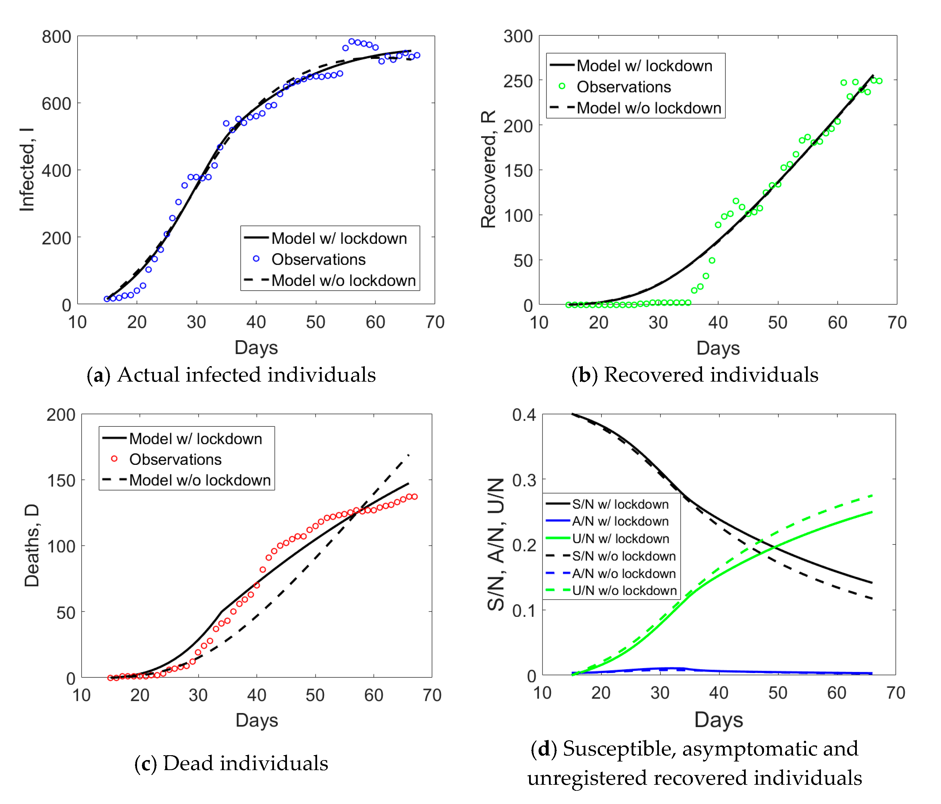
As far as Lombardy is concerned (Figure 7), lockdown measures were included after tLD = 18 (i.e., 21 days after the 21st of February). The effect of lockdown is especially pronounced on the compartment of actual infected individuals, whose trend cannot be captured by a model with time-independent parameters. Lockdown measures appear also to have been beneficial in terms of susceptible individuals, increasing their number as compared to the scenario without time-dependent parameters. Moreover, N0 was identified to be only 10% of the population size N. This implies that a release of social distancing measures should be done with care since 90% of the population could be still involved in future outbreaks.
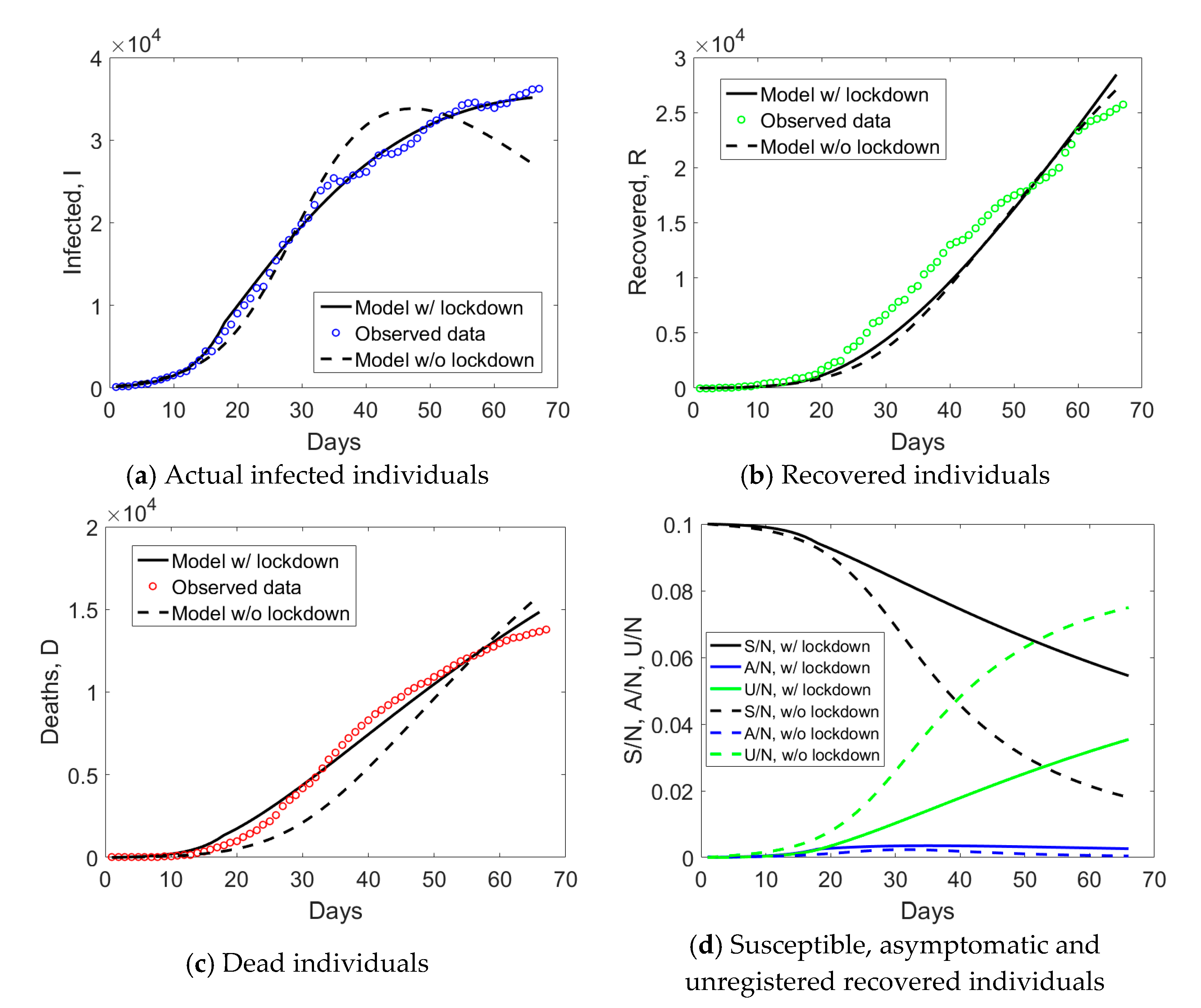
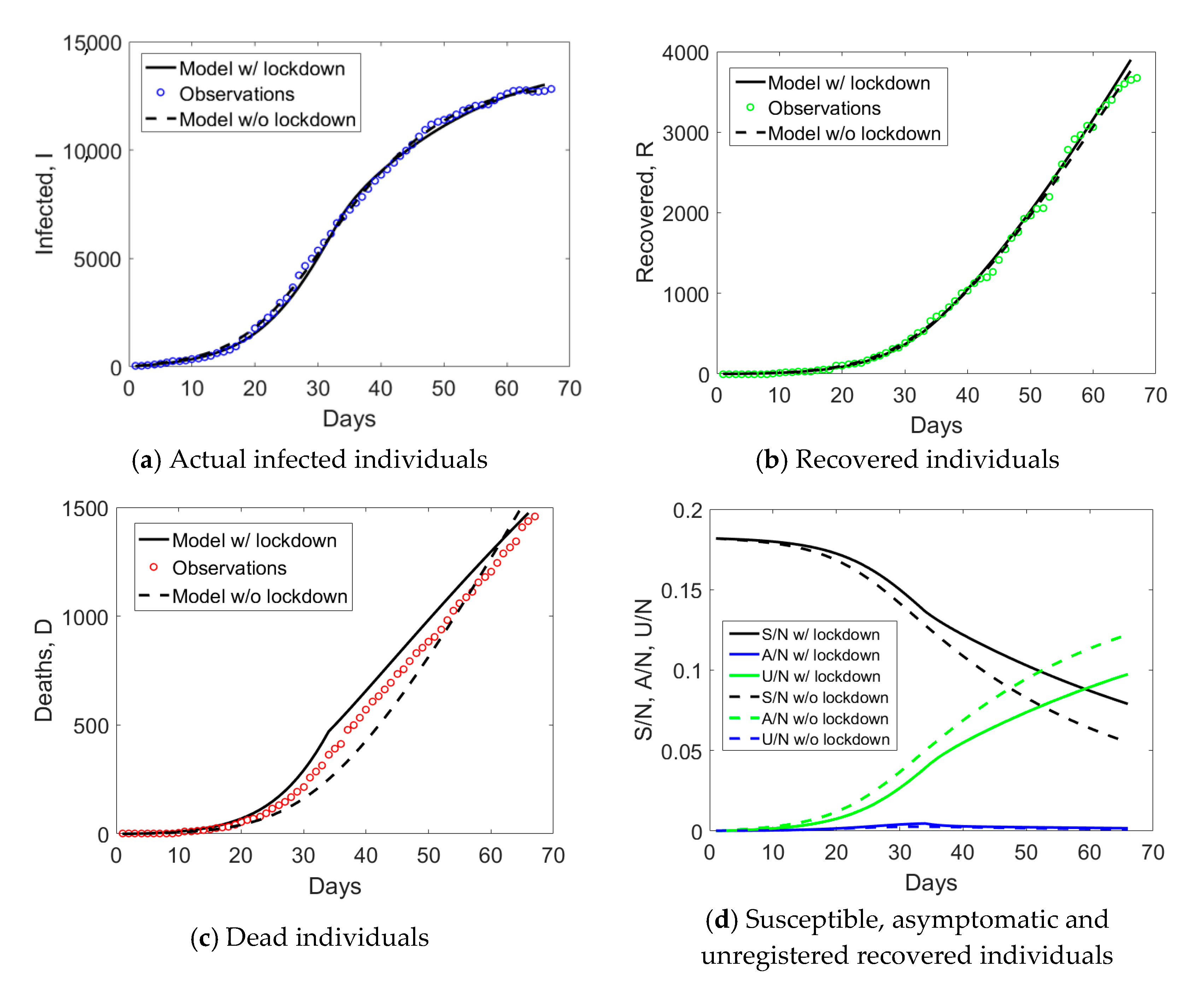
Results of the simulations for Emilia Romagna are shown in Figure 8. To model lockdown effects, tLD = 34 has been set, which corresponds to 21 days after the second Ministerial decree dated on 8 March, when the whole region was included in the “red zone”. Both simulations, with or without lockdown effects, using time-dependent or time-independent parameters, provide predictions close to the observed data, which means that a model with average parameters could be accurate enough to model the epidemic.
This could also imply that the impact of lockdown measures was not so strong as in Lombardy. In any case, the use of a time-dependent mortality rate led to major improvement of the model predictions, which became very close to the observed data (see Figure 8c). Based on the computations, the initial number of susceptible individuals is expected to be slightly above 15% for this region (see Figure 8d).
The result of the application of the proposed approach to Valle d’Aosta is shown in Figure 9, considering also in this case tLD = 34. Similar deductions for Emilia Romagna apply. The major difference regards the initial number of susceptible individuals, which is expected to have reached 40% for this region (see Figure 9d).
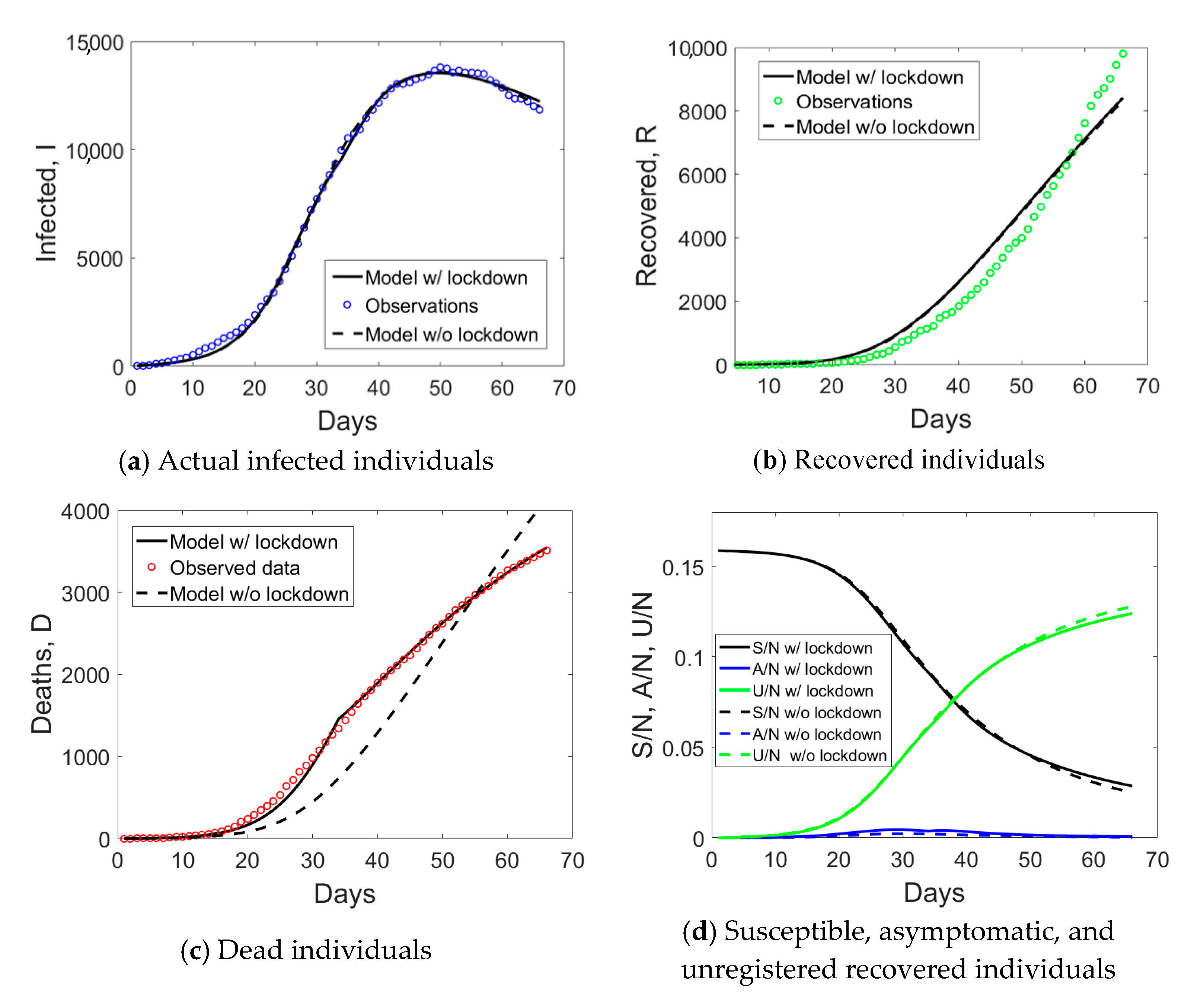
Finally, simulation results for Veneto are shown in Figure 10. Modeling the effect of lockdown measures using time-dependent parameters appears to be not so different as compared to using time-independent parameters, in line with the previously analyzed regions, with an exception for Lombardy. The number of initially susceptible individuals identified by the model is about 18% (see Figure 10d), which is similar to what was predicted for Emilia Romagna, a region of similar size, industrialization, and mobility infrastructures as Veneto.
All the identified model parameters for each region are collected in Table 1.
4. Discussion on Key Implications for Policymakers and Conclusions
The outcome of phase 1 in Italy has been analyzed starting from the observed data published by the Italian Civil Protection Centre. Lombardy, Emilia Romagna, Valle d’Aosta, and Veneto were examined since they were among the regions mostly affected by Covid-19 spreading. Moreover, due to their different characteristics in terms of population size, healthcare treatment policies, and lockdown measures, their comparisons provide important information for future actions of policymakers.
The analysis of the datasets showed the possibility that, for Valle d’Aosta and Veneto, the reported number of infected and recovered individuals could be overestimated, including also contributions from the asymptomatic compartments. Overestimation might lead to the erroneous indication to policymakers that the crisis is over and lockdown measures can be significantly released. For Valle d’Aosta, this expected overestimation can be motivated by the small population size of the region and the large number of medical swabs used not only to test individuals claiming for symptoms, but also to sample a large portion of the population. For Veneto, the cause can be attributed to the use of a laboratory testing machine that was available only there and that allowed a significant increase in the maximum number of daily processed medical swabs as compared to the other regions. Such a conjecture cannot be fully proved since the classification of the outcome of medical swabs in terms of compartments is still available by Istituto Superiore della Sanità only for a small number of samples. For the application of SIR models, where the distinction between I and A, and R and U compartments is crucial, it is highly recommended for public authorities to publish refined classifications distinguishing between symptomatic and asymptomatic cases. Massive testing of the whole population using medical swabs would clearly reduce the uncertainty in the observed data, and it should be highly recommended.
The machine learning approach herein proposed has been found to be robust for the identification of a large set of model parameters of the above epidemiological model which, albeit simple, included already five to seven parameters, depending whether lockdown effects with time-dependent parameters are included or not. In addition to those parameters, the initial number of susceptible individuals was not set equal to the population size, which is unrealistic due to the severity of lockdown measures that isolated at home many individuals, and it was identified by matching the observed R0 at the beginning of the epidemic.
Model results showed that lockdown measures had a major impact especially in Lombardy. For all the other regions, it was possible to achieve a relatively good match with observed data even using time-independent model parameters. The estimated number of susceptible individuals involved in the epidemic dynamics was found to be about 10% for Lombardy, 16% for Emilia Romagna, 18% for Veneto, and 40% for Valle d’Aosta. This means that lockdown was very effective. Nonetheless, such predictions imply further risk of contagion and outbreaks after releasing lockdown measures.
Future research directions might consider the extension of the present analysis to the post-lockdown period in Italy. Moreover, a systematic application of the proposed approach to Covid-19 data from other countries might be helpful in assessing the effect of different lockdown measures and healthcare policies on the pandemic spread, to draw general guidelines for policymakers. Finally, the generalization of the proposed epidemiological model to also deal with spatial dependent variables might be considered to simulate not only the time-evolution of the compartments, but also their spatial diffusion in the regions from localized outbreaks. In this regard, computational techniques based on the finite element method to solve reaction-diffusion problems [31] might be efficiently employed.
Funding
This research received no external funding.
Acknowledgments
M.P. would like to acknowledge the Young Academy of Europe that invited him to present the machine learning approach used in this study to a wide international audience in a symposium on COVID-19 epidemiology, held online on 22 April 2020, see https://meetings.yacadeuro.org/e/covid19.
Conflicts of Interest
The author declares no conflicts of interest.
References
- Boldog, P.; Tekeli, T.; Vizi, Z.; Dénes, A.; Bartha, F.; Röst, G. Risk assessment of novel coronavirus COVID-19 outbreaks outside China. J. Clin. Med. 2020, 9, 571. [Google Scholar] [CrossRef] [Green Version]
- Cheng, W.C.C.; Wong, S.-C.; To, K.K.W.; Ho, P.L.; Yuen, K.-Y. Preparedness and proactive infection control measures against the emerging Wuhan coronavirus pneumonia in China. J. Hosp. Infect. 2020, 104, 254–255. [Google Scholar] [CrossRef] [Green Version]
- Huang, C.; Wang, Y.; Li, X.; Ren, L.; Zhao, J.; Hu, Y.; Zhang, L.; Fan, G.; Xu, J.; Gu, X.; et al. Clinical features of patients infected with 2019 novel coronavirus in Wuhan, China. Lancet 2020, 395, 497–506. [Google Scholar] [CrossRef] [Green Version]
- Gatto, M.; Bertuzzo, E.; Mari, L.; Miccoli, S.; Carraro, L.; Casagrandi, R.; Rinaldo, A. Spread and dynamics of the COVID-19 epidemic in Italy: Effects of emergency containment measures. Proc. Natl. Acad. Sci. USA 2020, 117, 10484–10491. [Google Scholar] [CrossRef] [Green Version]
- Remuzzi, A.; Remuzzi, G. COVID-19 and Italy: What next? Lancet Health Policy 2020, 395, 1225–1228. [Google Scholar] [CrossRef]
- Kermack, W.O.; McKendrick, A.G. A contribution to the mathematical theory of epidemics. Proc. R. Soc. Lond. A 1927, 115, 700–721. [Google Scholar]
- Röst, G.; Wu, J. SEIR epidemiological model with varying infectivity and infinite delay. Math. Biosci. Eng. 2008, 5, 389–402. [Google Scholar]
- Montagnon, P. A stochastic SIR model on a graph with epidemiological and population dynamics occurring over the same time scale. J. Math. Biol. 2019, 79, 31–62. [Google Scholar] [CrossRef] [PubMed] [Green Version]
- Li, R.; Pei, S.; Chen, B.; Song, Y.; Zhang, T.; Yang, W.; Shaman, J. Substantial undocumented infection facilitates the rapid dissemination of novel coronavirus (SARS-CoV2). Science 2020, in press. [Google Scholar] [CrossRef] [PubMed] [Green Version]
- Yin Leung, K.; Trapman, P.; Britton, T. Who is the infector? Epidemic models with symptomatic and asymptomatic cases. Math. Biosci. 2018, 301, 190–198. [Google Scholar] [CrossRef] [PubMed]
- Gaeta, G. A simple SIR model with a large set of asymptomatic infectives. arXiv 2020, arXiv:2003.08720v1. [Google Scholar]
- Italian Civil Protection Centre. Open data on Covid-19 in Italy. Available online: https://github.com/ondata/covid19italia (accessed on 1 May 2020).
- Paggi, M. Simulation of Covid-19 epidemic evolution: Are compartmental models really predictive? arXiv 2020, arXiv:2004.08207. [Google Scholar]
- Tsiotas, D.; Magafas, L. The Effect of Anti-COVID-19 Policies on the Evolution of the Disease: A Complex Network Analysis of the Successful Case of Greece. Physics 2020, 2, 325–339. [Google Scholar]
- Schlickeiser, R.; Schlickeiser, F. A Gaussian Model for the Time Development of the Sars-Cov-2 Corona Pandemic Disease. Predictions for Germany Made on 30 March 2020. Physics 2020, 2, 164–170. [Google Scholar] [CrossRef]
- Schüttler, J.; Schlickeiser, R.; Schlickeiser, F.; Kröger, M. Covid-19 Predictions Using a Gauss Model, Based on Data from April 2. Physics 2020, 2, 197–212. [Google Scholar]
- Baker, R. Reactive social distancing in a SIR model of epidemics such as COVID-19. arXiv 2020, arXiv:2003.08285. [Google Scholar]
- Ibarra-Vega, D. Lockdown, one, two, none, or smart. Modeling containing covid-19 infection. A conceptual model. Sci. Total Environ. 2020, 730, 138917. [Google Scholar] [CrossRef]
- Whitley, D. A genetic algorithm tutorial. Stat. Comput. 1994, 4, 65–85. [Google Scholar] [CrossRef]
- Price, K.V. Differential evolution. In Handbook of Optimization; Springer: Berlin/Heidelberg, Germany, 2013; pp. 187–214. [Google Scholar]
- Carollo, V.; Piga, D.; Borri, C.; Paggi, M. Identification of elasto-plastic and nonlinear fracture mechanics parameters of silver-plated copper busbars for photovoltaics. Eng. Fract. Mech. 2019, 205, 439–454. [Google Scholar] [CrossRef]
- Zhang, H. Transient performance of the Particle Swarm Optimization algorithm from system dynamics point of view. J. Comput. Inf. Sci. Eng. 2020, 20, 041008. [Google Scholar] [CrossRef]
- Prasad, J.; Souradeep, T. Cosmological parameter estimation using particle swarm optimization. Phys. Rev. D 2012, 85, 123008. [Google Scholar] [CrossRef] [Green Version]
- Zhang, S.; Gong, J. Floquet engineering with particle swarm optimization: Maximizing topological invariants. Phys. Rev. B 2019, 100, 235452. [Google Scholar] [CrossRef] [Green Version]
- Glück, A.; Hüffel, H.; Ilijić, S. Swarms with canonical active Brownian motion. Phys. Rev. E 2011, 83, 051105. [Google Scholar] [CrossRef] [PubMed] [Green Version]
- Li, Y.; Cheng, W.; Yu, L.H.; Rainer, R. Genetic algorithm enhanced by machine learning in dynamic aperture optimization. Phys. Rev. Accel. Beams 2018, 21, 054601. [Google Scholar] [CrossRef] [Green Version]
- Fontanari, J.F. Social interaction as a heuristic for combinatorial optimization problems. Phys. Rev. E 2010, 82, 056118. [Google Scholar] [CrossRef] [PubMed] [Green Version]
- Li, W.; Zhang, H.-T.; Chen, M.Z.; Zhou, T. Singularities and symmetry breaking in swarms. Phys. Rev. E 2008, 77, 021920. [Google Scholar] [CrossRef] [Green Version]
- Fan, S.-K.S.; Lin, Y. A fast estimation method for the generalized Gaussian mixture distribution on complex images. Comput. Vis. Image Underst. 2009, 113, 839–853. [Google Scholar] [CrossRef]
- Wang, D.; Tan, D.; Liu, L. Particle swarm optimization algorithm: An overview. Soft Comput. 2018, 22, 387–408. [Google Scholar] [CrossRef]
- Lenarda, P.; Paggi, M.; Ruiz Baier, R. Partitioned coupling of advection–diffusion–reaction systems and Brinkman flows. J. Comput. Phys. 2017, 344, 281–302. [Google Scholar] [CrossRef] [Green Version]
Figure 1.
Observed compartments (a) and daily rates of dead and recovered individuals (b) in Lombardy, from 24 February 2020 (day 1) till 30 April 2020 (day 67).
Figure 1.
Observed compartments (a) and daily rates of dead and recovered individuals (b) in Lombardy, from 24 February 2020 (day 1) till 30 April 2020 (day 67).

Figure 2.
Observed compartments (a) and daily rates of dead and recovered individuals (b) in Emilia Romagna from 24 February 2020 (day 1) till 30 April 2020 (day 67).
Figure 2.
Observed compartments (a) and daily rates of dead and recovered individuals (b) in Emilia Romagna from 24 February 2020 (day 1) till 30 April 2020 (day 67).

Figure 3.
Observed compartments (circles) in Valle d’Aosta and proposed corrected values based on the ratio between the daily total number of medical swabs over the number of actual infectious individuals (pentagrams) from 24 February 2020 (day 1) till 30 April 2020 (day 67).
Figure 3.
Observed compartments (circles) in Valle d’Aosta and proposed corrected values based on the ratio between the daily total number of medical swabs over the number of actual infectious individuals (pentagrams) from 24 February 2020 (day 1) till 30 April 2020 (day 67).

Figure 4.
Ratio between the total number of medical swabs and the actual number of infected individuals, I (a), and daily rates of dead and recovered individuals (b) in Valle d’Aosta from 24 February 2020 (day 1) till 30 April 2020 (day 67).
Figure 4.
Ratio between the total number of medical swabs and the actual number of infected individuals, I (a), and daily rates of dead and recovered individuals (b) in Valle d’Aosta from 24 February 2020 (day 1) till 30 April 2020 (day 67).

Figure 5.
Observed compartments (circles) in Veneto and proposed corrected values based on the ratio between the daily total number of medical swabs over the number of actual infected individuals (pentagrams) from 24 February 2020 (day 1) till 30 April 2020 (day 67).
Figure 5.
Observed compartments (circles) in Veneto and proposed corrected values based on the ratio between the daily total number of medical swabs over the number of actual infected individuals (pentagrams) from 24 February 2020 (day 1) till 30 April 2020 (day 67).

Figure 6.
Ratio between the total number of medical swabs and the actual number of infected individuals, I (a), and daily rates of dead and recovered individuals (b) in Veneto from 24 February 2020 (day 1) till 30 April 2020 (day 67).
Figure 6.
Ratio between the total number of medical swabs and the actual number of infected individuals, I (a), and daily rates of dead and recovered individuals (b) in Veneto from 24 February 2020 (day 1) till 30 April 2020 (day 67).

Figure 7.
Simulated compartments including or excluding lockdown measures in the model, for Lombardy.
Figure 7.
Simulated compartments including or excluding lockdown measures in the model, for Lombardy.

Figure 8.
Simulated compartments including or excluding lockdown measures in the model, with time-dependent or time-indepedent parameters, for Emilia Romagna.
Figure 8.
Simulated compartments including or excluding lockdown measures in the model, with time-dependent or time-indepedent parameters, for Emilia Romagna.

Figure 9.
Simulated compartments including or excluding lockdown measures in the model, with time-dependent or time-independent parameters, for Valle d’Aosta.
Figure 9.
Simulated compartments including or excluding lockdown measures in the model, with time-dependent or time-independent parameters, for Valle d’Aosta.

Figure 10.
Simulated compartments including or excluding lockdown measures in the model, with time-dependent or time-independent parameters, for Veneto.
Figure 10.
Simulated compartments including or excluding lockdown measures in the model, with time-dependent or time-independent parameters, for Veneto.


Table 1.
Summary of the identified model parameters.
| Region | β0 | γ | μ0 | η | ξ | ρ | ρm | N0/N |
|---|---|---|---|---|---|---|---|---|
| Lombardy | 0.4191 | 0.0226 | 0.0398 | 0.2159 | 0.1654 | 1.8 × 10⁻⁵ | 0.6552 | 10% |
| Reggio Emilia | 1.0219 | 0.0017 | 0.0165 | 0.9418 | 0.0417 | 4.5 × 10⁻⁶ | 0.4536 | 16% |
| Valle d’Aosta | 0.8843 | 0.0103 | 0.0133 | 0.8271 | 0.0351 | 8.7 × 10⁻⁵ | 0.6103 | 40% |
| Veneto | 0.7700 | 0.0097 | 0.0077 | 0.7159 | 0.0364 | 7.8 × 10⁻⁶ | 0.5646 | 18% |
© 2020 by the author. Licensee MDPI, Basel, Switzerland. This article is an open access article distributed under the terms and conditions of the Creative Commons Attribution (CC BY) license (http://creativecommons.org/licenses/by/4.0/).
Share and Cite
MDPI and ACS Style
Paggi, M. An Analysis of the Italian Lockdown in Retrospective Using Particle Swarm Optimization in Machine Learning Applied to an Epidemiological Model. Physics 2020, 2, 368-382. https://0-doi-org.brum.beds.ac.uk/10.3390/physics2030020
AMA Style
Paggi M. An Analysis of the Italian Lockdown in Retrospective Using Particle Swarm Optimization in Machine Learning Applied to an Epidemiological Model. Physics. 2020; 2(3):368-382. https://0-doi-org.brum.beds.ac.uk/10.3390/physics2030020
Chicago/Turabian StylePaggi, Marco. 2020. "An Analysis of the Italian Lockdown in Retrospective Using Particle Swarm Optimization in Machine Learning Applied to an Epidemiological Model" Physics 2, no. 3: 368-382. https://0-doi-org.brum.beds.ac.uk/10.3390/physics2030020