Scattering of Lower Hybrid Waves in a Magnetized Plasma

Abstract

In this paper, the Maxwell equations for the electric field in a cold magnetized plasma in the half-space of $x\ge 0$ cm are solved. The boundary conditions for the electric field include a pointwise source at the plane $x=0$ cm, the derivatives of the electric field that are zero statV/cm${}^2$ at $x=0$ cm, and the field with all its derivatives that are zero at infinity. The solution is explored in terms of the Laplace transform in x and the Fourier transform in y-z directions. The expressions of the field components are obtained by the inverse Laplace transform and the inverse Fourier transform. The saddle-point technique and power expansion have been used for evaluating the inverse Fourier transform. The model represents the propagation of a lower hybrid wave generated by a pointwise antenna located at the boundary of the plasma. Here, the antenna is the boundary condition. The validation of the model is performed assuming that the electric field component $E_y=0$ statV/cm and by comparing it with the model of electromagnetic waves generated by a local small antenna located near the boundary of a tokamak, and an experiment is suggested.

1. Introduction

In order to study the propagation of an electromagnetic (EM) wave inside the boundary of a tokamak, where the cold plasma approximation can be performed, we solve the Maxwell equations for a wave generated by a small antenna outside the plasma. In the first approach, the antenna is considered a point-like source. In a more realistic approach, we consider a small antenna that serves as a point of comparison with other theories and shows the connection with experiments. Here, we suppose that the density and temperature are constant. Thus, the present study is a first attempt towards the development of diagnostics based on the onset of parametric instabilities driven by lower hybrid (LH) waves (LHWs). They change the frequency spectra of the injected waves, broadening them and possibly producing satellites separated by a gap given by the ion cyclotron frequency [1,2]. The radio frequency (RF) spectra can be measured by RF probes located outside the vessel. Since these spectra depend on the detail of the density and temperature profiles, the latter can be inferred. The power threshold for parametric instabilities is typically of the order of a few tens of kW. Therefore, a relatively small LH antenna can be used for such diagnostics with poor occupation of the available accesses to the plasma across the vessel. Traditional reciprocating Langmuir probes used to measure the density and temperature profiles against time need multiple scans inside the plasma. Their use in reactor relevant devices is, in any case, prevented by the harmful conditions of the peripheral plasma and is not suitable for the use in reciprocating Langmuir probes. Conversely, a relatively small antenna located against the vessel wall is compatible with such conditions and can provide a better time resolution than the reciprocating Langmuir probes.

The Maxwell equations describing the propagation of an electromagnetic wave in a plasma, in the presence of an external magnetic field, have an easily worked form when the frequencies of the electric field are much higher than the ion cyclotron frequencies in the plasma, because the cold plasma assumption is satisfied for the plasma dielectric tensor. A coupled system of partial differential equations in space can be obtained for an EM field whose frequency is fixed by the antenna generator. Nevertheless, a proper solution of this equation system with suitable boundary values appears to be extremely complicated in a very simple geometry including a reduced model for the plasma density and magnetic field, which can be taken as constant all over the plasma space in the first attempt. This last assumption can be naively justified considering that the wavelength involved in the process satisfies the inequality $\lambda \ll L$, where L is the variation scale length of the macroscopic plasma parameters of density and confining magnetic field. In this framework it is quite appealing to try to apply asymptotic methods using the formulations given in [3,4,5,6,7]. We used the saddle-point technique [8] and an expansion with respect to a small parameter.

The paper is divided into several sections. In Section 2, there is brief description of the general derivation of the wave equation in a cold plasma. In Section 3, a discussion of the peculiarity of the Maxwell equation for this model is developed and some simplifying hypotheses are assumed. There is a manipulation of the wave equation by the Fourier–Laplace transform. We then obtain the general dispersion relation for the solution generated by a pointwise boundary condition and compute the values of components of the electric field in Section 4. In Section 5, we validate this model assuming more physical hypotheses, such as a model of a wave generated by a small antenna generalizing the model with a point-like source. We solve this model using the same analytical method, compare it with existing theoretical and experimental results, and propose an experiment. Finally, conclusions are presented in Section 6.

2. Derivation of the Main Equations

Here, we use non-dimensional variables and the CGS unit system with $\mathbf{B}\equiv \mathbf{B}/B_0$, $B_0=1$ G, $\mathbf{E}(r,t)\equiv \mathbf{E}(r,t)/E_0$, $E_0=1$ statV/cm (statVolt/cm), charge $q_{\alpha }\equiv q_{\alpha }/q_0$, $\alpha =i,e$ ($i=$ ion, $e=$ electron), $q_0=1$ esu, $\mathbf{r}\equiv \mathbf{r}/r_0$, $r_0=1$ cm, $n_{\alpha }\equiv n_{\alpha }/n_0$, $n_0=1$ cm${}^{-3}$, $t\equiv t/t_0$, $t_0=1$ s, $\omega \equiv \omega /{\omega }_0$, ${\omega }_0=1$ rad/s, and $m_{\alpha }\equiv m_{\alpha }/m_0,$$m_0=1$ g. The defining constants are the charges $q_{\alpha }$, the masses $m_{\alpha }$, and the densities $n_{\alpha }$. The Maxwell equations for the electric field $\mathbf{E}(\mathbf{r},t)$ of a wave propagating in such a medium are

$$\overrightarrow{\nabla }\wedge \overrightarrow{\nabla }\wedge \mathbf{E}(\mathbf{r},t)+\frac{1}{c^2}(\frac{{\partial }^2}{\partial t^2}\mathbf{E}(\mathbf{r},t)+4\pi \sum _{\alpha =i,e}{q}_{\alpha }{n}_{\alpha }\frac{\partial {\mathbf{V}}_{\alpha }}{\partial t})=0,$$

(1)

where $c\equiv c/c_0$, $c_0=1$ cm/s and c is the velocity of the light. The current density has been replaced by the constitutive relation $\mathbf{j}={\sum }_{\alpha }{n}_{\alpha }{q}_{\alpha }{\mathbf{V}}_{\alpha }$$\mathbf{j}\equiv \mathbf{j}/j_0$, $j_0=1$ stamps cm${}^{-3}$, where $q_{\alpha }{n}_{\alpha }$ and ${\mathbf{V}}_{\alpha }$ are the charge density and fluid velocity, respectively, and ${\mathbf{V}}_{\alpha }\equiv {\mathbf{V}}_{\alpha }/V_0$, $V_0=1$ cm/s. This system of equations is coupled with the linearized fluid equations of momentum conservation for the two types of charged particles such that we obtain the following system of equations:

$$\left\{\begin{array}{c}\nabla \wedge \nabla \mathbf{E}(\mathbf{r},t)+\frac{1}{c^2}(\frac{{\partial }^2}{\partial t^2}\mathbf{E}(\mathbf{r},t)+4\pi \sum _{\alpha =i,e}{q}_{\alpha }{n}_{\alpha }\frac{\partial {\mathbf{V}}_{\alpha }}{\partial t})=0\hfill \\ \frac{\partial {\mathbf{V}}_{\alpha }}{\partial t}=\frac{q_{\alpha }}{m_{\alpha }}\mathbf{E}+{\Omega }_{\alpha }{\mathbf{V}}_{\alpha }\wedge \mathbf{b},\alpha =i,e,\hfill \end{array}\right.$$

(2)

where, in the first equation of the system (2), we have considered a constant plasma density $n={10}^{12}$${\mathrm{cm}}^{-3}$ and ${\mathbf{V}}_{\alpha }$ is the velocity and is essentially neglected at the lowest order of the nonlinear terms. We have introduced the cyclotron frequencies as

$${\Omega }_{\alpha }=\frac{q_{\alpha }\left|\mathbf{B}\right|}{m_{\alpha }c},$$

which we can consider constant in space and where $\mathbf{b}$ is the unit vector parallel to $\mathbf{B}$. Considering a harmonic representation of the perturbed quantities,

$${\mathbf{V}}_{\alpha }={\mathbf{V}}_{0\alpha }{e}^{i\omega t}$$

and

$$\mathbf{E}(\mathbf{r},t)={\mathbf{E}}_0\left(\mathbf{r}\right)e^{i\omega t},$$

where $\omega$ represents the frequency of the wave. Thus, Equation (2) can be written compactly as

$$-{\omega }^2{\mathbf{E}}_0+c^2\nabla \wedge \nabla \wedge {\mathbf{E}}_0+4\pi i\omega \underline{\underline{\sigma }}\times {\mathbf{E}}_0=0,$$

(3)

where $\underline{\underline{\sigma }}$ is the conductivity tensor and × indicates the product of a tensor with a vector. We can write Equation (3) more compactly by introducing the dielectric tensor in the cold plasma case as

$$\underline{\underline{\tau }}=\underline{\underline{I}}+4\pi i\frac{1}{\omega }\underline{\underline{\sigma }}$$

and

$$c^2\nabla \wedge \nabla \wedge {\mathbf{E}}_0-{\omega }^2\underline{\underline{\tau }}\times {\mathbf{E}}_0=0.$$

(4)

The elements of the dielectric tensor are usually given in terms of Stix’s notation [9] as

$$\left\{\begin{array}{c}{\tau }_{xx}={\tau }_{yy}=S=1-\sum _{\alpha }\frac{{\omega }_{p\alpha }^2}{{\omega }^2-{\Omega }_{c\alpha }^2},\hfill \\ {\tau }_{xy}=-{\tau }_{yx}=-iD=-i\sum _{\alpha }\frac{{\omega }_{p\alpha }^2}{{\omega }^2-{\Omega }_{c\alpha }^2}\frac{{\Omega }_{c\alpha }^2}{\omega },\hfill \\ {\tau }_{zz}=P=1-\sum _{\alpha }\frac{{\omega }_{p\alpha }^2}{{\omega }^2},\hfill \end{array}\right.$$

(5)

while

$${\tau }_{xz}={\tau }_{zx}={\tau }_{zy}={\tau }_{yz}=0.$$

In Equation (5) we have also introduced the plasma frequencies of particles of type $\alpha$

$${\omega }_{p\alpha }=\sqrt{\frac{4\pi q_{\alpha }{n}_{\alpha }}{m_{\alpha }}},$$

while the cyclotron frequency ${\Omega }_{c\alpha }$ has been defined above. The solution of Equation (4), with some prescribed boundary conditions at the plasma surface, describes the propagation of an electromagnetic wave inside the plasma volume. As stated in the introduction, we are interested in the propagation of the waves in the high frequency limit

$${\Omega }_{ce}>>\omega >>{\Omega }_{ci}$$

wherein the frequency domain is much higher than the ion cyclotron frequency and much lower than the electron cyclotron frequency, for which Equation (4) is compatible with the plasma model we have used (cold and magnetized plasma).

3. Fourier-Laplace Transform

As we want to solve the following system of PDE (Partial Differential Equation), let $\mathbf{E}=(E_x,E_y,E_z)$ and the magnetic field be parallel to the z axis, then

$$\left\{\begin{array}{c}-\frac{\partial }{\partial z}[\frac{\partial }{\partial z}{E}_x-\frac{\partial }{\partial x}{E}_z]+\frac{\partial }{\partial y}[\frac{\partial }{\partial x}{E}_y-\frac{\partial }{\partial y}{E}_x]-\frac{{\omega }^2}{c^2}[S{E}_x-iD{E}_y]=0,\hfill \\ -\frac{\partial }{\partial x}[\frac{\partial }{\partial x}{E}_y-\frac{\partial }{\partial y}{E}_x]+\frac{\partial }{\partial z}[\frac{\partial }{\partial y}{E}_z-\frac{\partial }{\partial z}{E}_y]-\frac{{\omega }^2}{c^2}[iD{E}_x-S{E}_y]=0,\hfill \\ -\frac{\partial }{\partial y}[\frac{\partial }{\partial y}{E}_z-\frac{\partial }{\partial z}{E}_y]+\frac{\partial }{\partial x}[\frac{\partial }{\partial z}{E}_x-\frac{\partial }{\partial x}{E}_z]-\frac{{\omega }^2}{c^2}\left[P{E}_x\right]=0.\hfill \end{array}\right.$$

(6)

The system is considered in the domain $x\ge 0,-\infty \le y\le \infty ,-\infty \le z\le \infty$. The field components at $x=0$ are given by a pointwise localized field

$$\mathbf{E}(0,y,z)={\mathbf{E}}_0\delta \left(y\right)\delta \left(z\right)$$

(7)

and the field $\mathbf{E}\to 0$ together with its derivatives for $\mathbf{x}\to \infty$. ${\mathbf{E}}_0(0,y,z)$ is the electric field in the plane $x=0$ cm generated by the antenna and the plasma is located in the half-space $x>0$ cm. The derivatives of $\mathbf{E}(x,y,z)$ at $x=0$ cm are 0 statV/cm${}^2$. This field is an electrical field generated by a point source located at the boundary of the plasma.

Given the structure of this domain, we have to make a Laplace transform in x and a Fourier transform in y and z in order to solve the linear system of second-order partial derivatives in Equation (6):

$$\mathbf{E}(s,k_y,k_z)=\frac{1}{2\pi }{\int }_0^{\infty }dxexp(-sx)\int dydzexp(-i{k}_{y}y-i{k}_{z}z)\mathbf{E}(x,y,z),$$

(8)

where $s\equiv s/s_0$, $k_y\equiv k_y/k_0$, $k_z\equiv k_z/k_0$, and $s_0$ and $k_0=1$ cm${}^{-1}$. Making the transformation and taking the density as constant, we obtain the equations

$$\begin{array}{c}\hfill \left(\begin{array}{ccc}{k}_y^2+k_z^2-\frac{S{\omega }^2}{c^2}& i\left(\frac{D{\omega }^2}{c^2}-s{k}_y\right)& -is{k}_z\\ -i\left(s{k}_y+\frac{D{\omega }^2}{c^2}\right)& -s^2+k_z^2-\frac{S{\omega }^2}{c^2}& -k_y{k}_z\\ -is{k}_z& k_y{k}_z& -s^2+k_y^2-\frac{P{\omega }^2}{c^2}\end{array}\right)\times \left(\begin{array}{c}{E}_x\\ E_y\\ E_z\end{array}\right)\end{array}$$

(9)

$$\begin{array}{c}\hfill =\left(\begin{array}{c}i(k_z+k_y)\\ -s-i{k}_y\\ -s\end{array}\right),\end{array}$$

(10)

where P, S, and D are the components of the dielectric tensor using Stix’s notation [9]. Then, we list the various assumptions of the model as follows:

• We deal with the deuterium plasma zone near the boundary of the tokamak.
• $B\equiv (0,0,B)$ with $B=5$ T.
• The Stix coefficients are

  $$S\left(\omega \right)=1-{\Sigma }_{\alpha =e,i}{\omega }_{p\alpha }^2/({\omega }^2-{\Omega }_{c\alpha }^2).$$
• Plasma density $n={10}^{12}$ cm${}^{-3}.$
• $$P\left(\omega \right)=1-{\Sigma }_{\alpha =e,i}{\omega }_{p\alpha }^2/{\omega }^2.$$
• $$D\left(\omega \right)={\Sigma }_{\alpha =e,i}\frac{{\omega }_{p\alpha }^2}{\omega }\frac{{\Omega }_{c\alpha }}{{\omega }^2-{\Omega }_{c\alpha }^2}.$$
• ${\Omega }_{ce}=-8.79\times {10}^{11}$ rad/s is the electron cyclotron frequency.
• ${\Omega }_{ci}=2.4\times {10}^8$ rad/s is the ion cyclotron frequency.
• ${\omega }_{pe}=5.64\times {10}^{10}$ rad/s is the electron plasma frequency.
• ${\omega }_{pi}=9.3\times {10}^8$ rad/s is the ion plasma frequency.
• $\mathbf{E}(0,y,z)=(0,1,1)\delta \left(y\right)\delta \left(z\right)$ statV/cm are the boundary conditions (b.c.) for the electric field on the $x=0$ cm plane and the derivatives on this plane are zero. The field, together with its derivatives, is zero at infinity. The value of the field at $x=0$ cm is not relevant for our calculations. However, the $(0,1,1)$ statV/cm condition has been chosen because it gives interesting results. A boundary condition of the type $(1,1,1)$ statV/cm gives rise to unstable and diverging solutions. So, the problem is stiff with respect to the choice of the b.c.
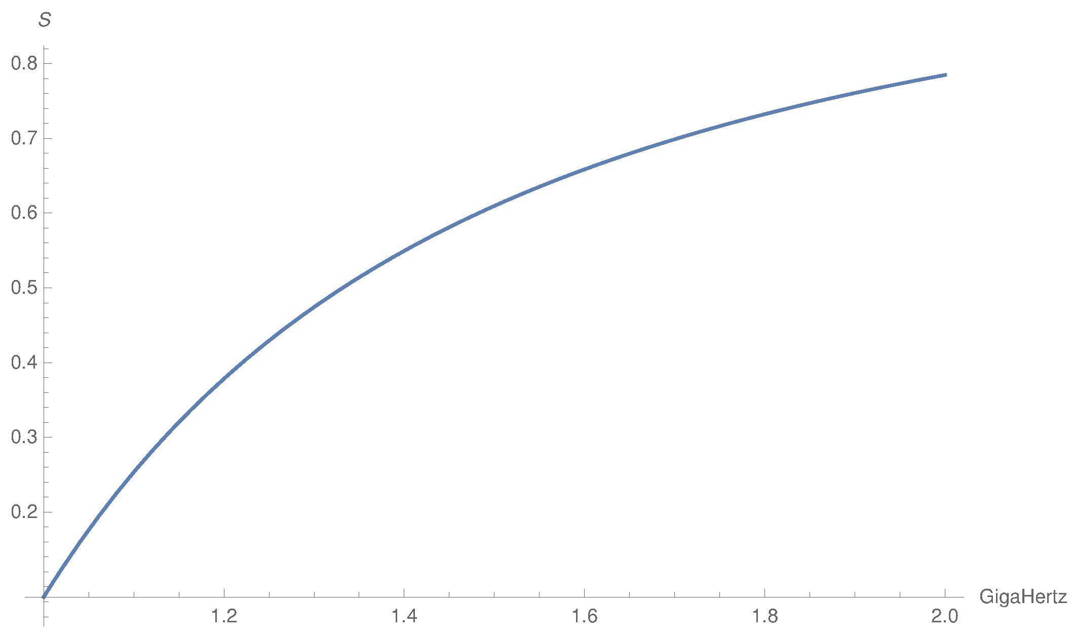
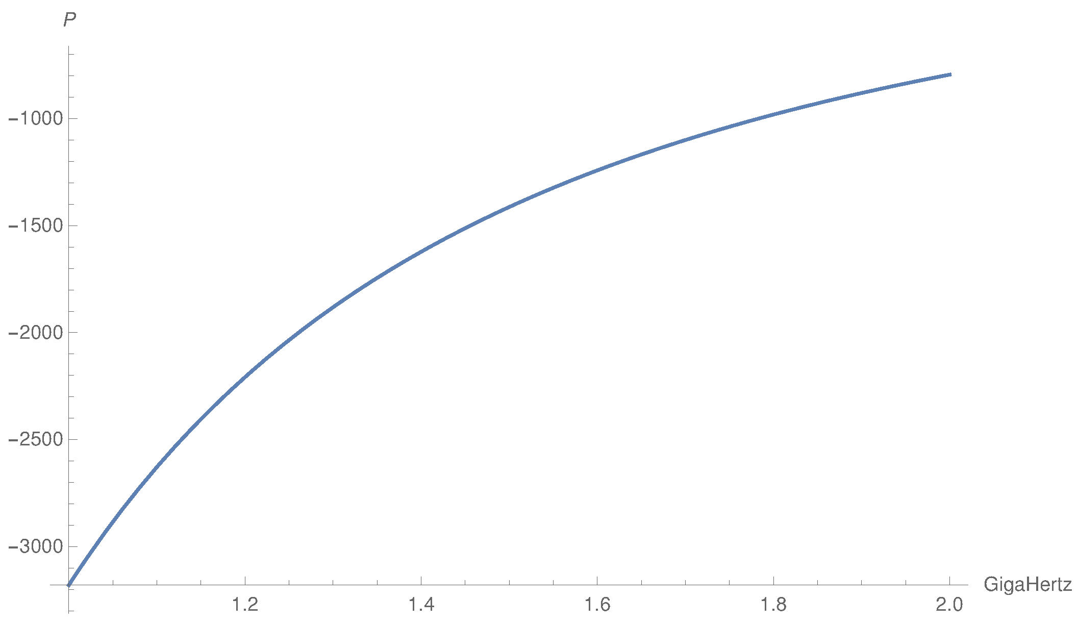
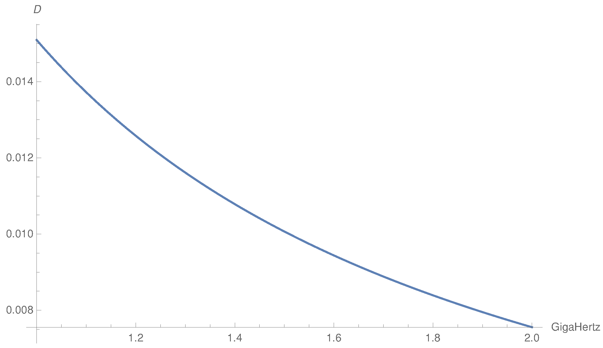
• We neglect D and keep only S and P in the transformed matrix. P is three orders of magnitude larger than S and and four orders of magnitude larger than D in the frequency range $\omega \in (1\times {10}^9,2\times {10}^9)$ Hz as one can see from Figure 1, Figure 2 and Figure 3. If we set $S=0$, we get a divergent behavior of the field as it is possible to check from the final formulas for the components of $\mathbf{E}$. So, the problem is also stiff with respect to the possible approximations of S, D, and P.
• We study the propagation only in the $(x,z)$ plane, so we set $k_y=0$ cm${}^{-1}$ and $k_z=k$.

The right-hand side of this system comes from the Laplace transforms of the first- and second-order derivatives with respect to x. Thus, we have the following Laplace transforms:

$${\int }_0^{\infty }{e}^{-sx}\frac{\partial \mathbf{E}(x,0,k)}{\partial x}dx=-\mathbf{E}(0,0,k)+s\mathbf{E}(s,0,k),$$

$${\int }_0^{\infty }{e}^{-sx}\frac{{\partial }^2\mathbf{E}(x,0,k)}{\partial x^2}dx=-s\mathbf{E}(0,0,k)+s^2\mathbf{E}(s,0,k).$$

Using the above assumptions, we get the system

$$\begin{array}{c}\hfill \left(\begin{array}{ccc}{k}^2-\frac{S{\omega }^2}{c^2}& i\frac{D{\omega }^2}{c^2}& -isk\\ -i\frac{D{\omega }^2}{c^2}& -s^2+k^2-\frac{S{\omega }^2}{c^2}& 0\\ -isk& 0& -s^2-\frac{P{\omega }^2}{c^2}\end{array}\right)\times \left(\begin{array}{c}{E}_x\\ E_y\\ E_z\end{array}\right)\end{array}$$

(11)

$$\begin{array}{c}\hfill =\left(\begin{array}{c}ik\\ -s\\ -s\end{array}\right).\end{array}$$

(12)

Finally, we plot the graphs of the three functions S, P, and D in Figure 1, Figure 2 and Figure 3, respectively; we use GigaHertz (GHz) $={10}^9$ rad/s.

4. Computation of the Transformed Electric Field

The transformed component of the electric field can easily be derived from the system in Equation (11). For a simpler representation of the formulae, we set $P^{\prime }=\frac{{\omega }^2}{c^2}P\to P$, $S^{\prime }=\frac{{\omega }^2}{c^2}S\to S$, and $k=k_z$, as well as $\mathbf{E}(s,0,k)=\mathbf{E}(s,k)=(E_x(s,k),E_y(s,k),E_z(s,k)$. From the second equation, we get

$$E_y(s,0,k)=-\frac{s}{k^2-S-s^2},$$

(13)

where the first and third equations give

$$E_x=-ik\frac{2s^2+P}{k^2{s}^2-(s^2+P)(k^2-S)}$$

(14)

and

$$E_z=-\frac{s(2k^2-S)}{k^2{s}^2-(s^2+P)(k^2-S)}.$$

(15)

Here, we give the results of the antitransformations and in Appendix A, one can find the respective derivations.

4.1. $E_y$ Component

Making the inverse Laplace transform of

$$E_y(s,0,k)=-\frac{s}{k^2-S-s^2},$$

(16)

we obtain $E_y(x,k)$ and

$$E_y(x,k)=1/2(e^{-x\sqrt{k^2-S}}+e^{x\sqrt{k^2-S}}).$$

(17)

In order to avoid divergent behavior, we drop the $e^{x\sqrt{k^2-S}}$ term. The component $E_y$ is obtained making the inverse Fourier transform as it is shown in Appendix A.1 and as follows

$$E_y(x,z)=1/\left(2\sqrt{2\pi }\right)\int e^{ikz-x\sqrt{k^2-S}}dk.$$

(18)

Using the saddle-point method, we get a complex function $E_y(x,z)$ and are interested in the real part as follows:

$$\mathrm{Re}{E}_y(x,z)=cos(\frac{(z^2-x^2)\sqrt{S}}{x^2+z^2}+\pi /4)S^{1/4}x{(x^2+z^2+{10}^{-3})}^{-3/4}.$$

(19)

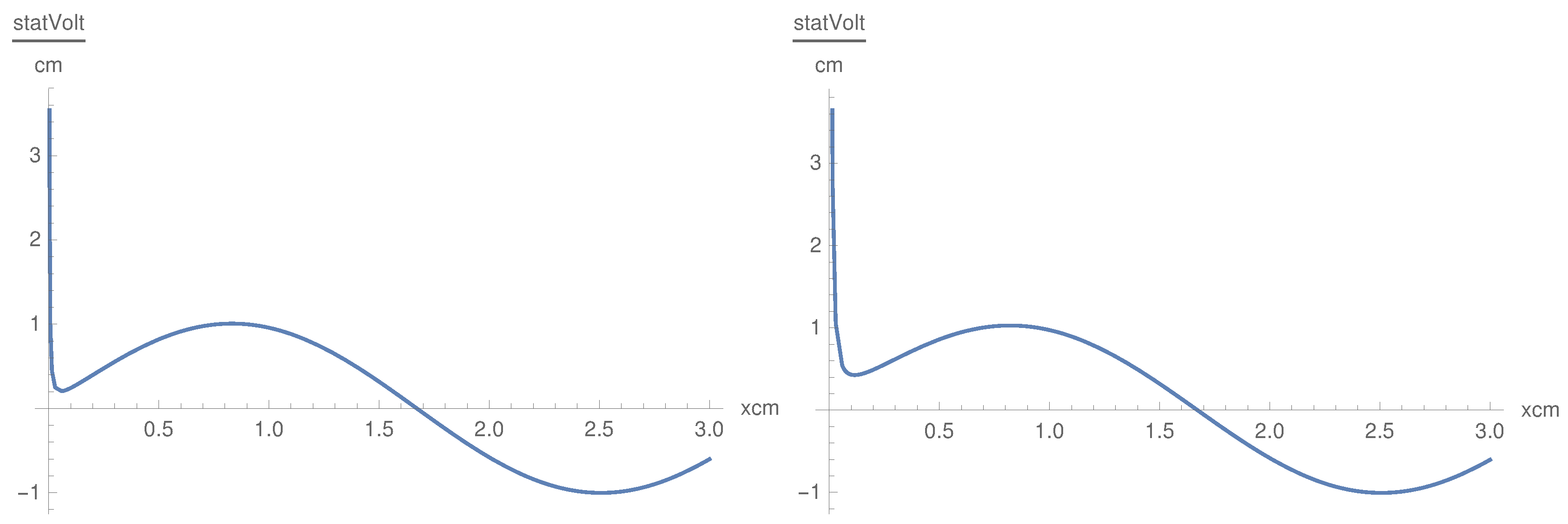
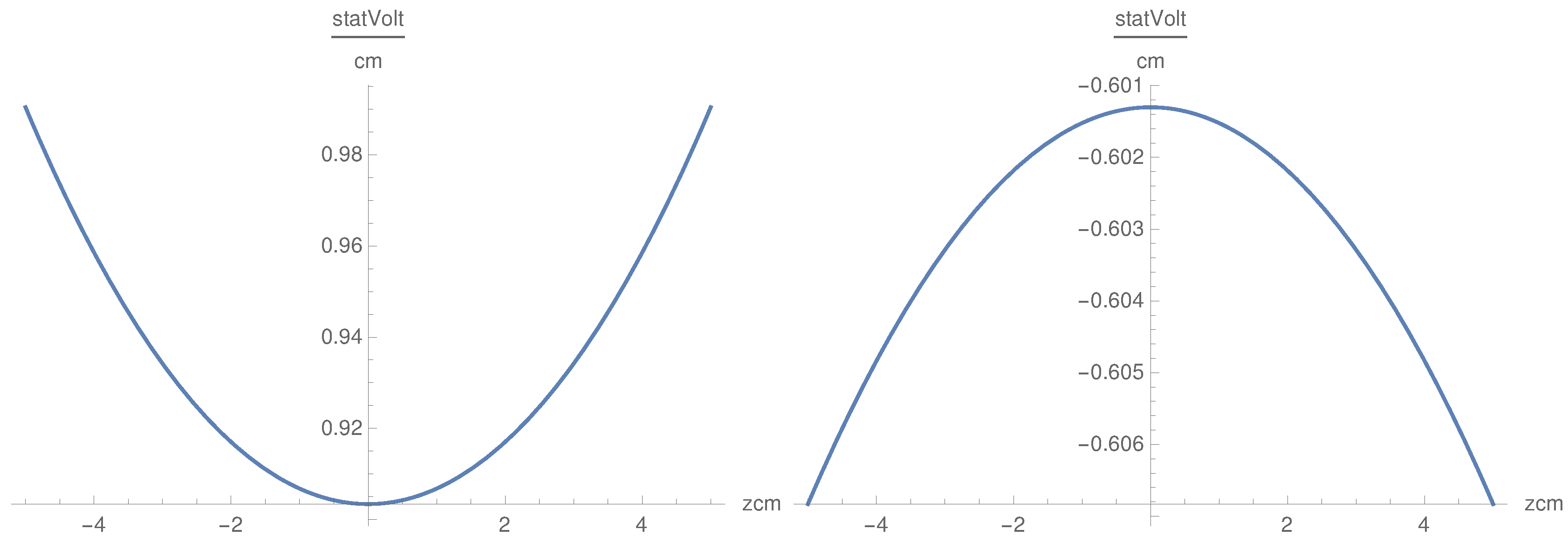
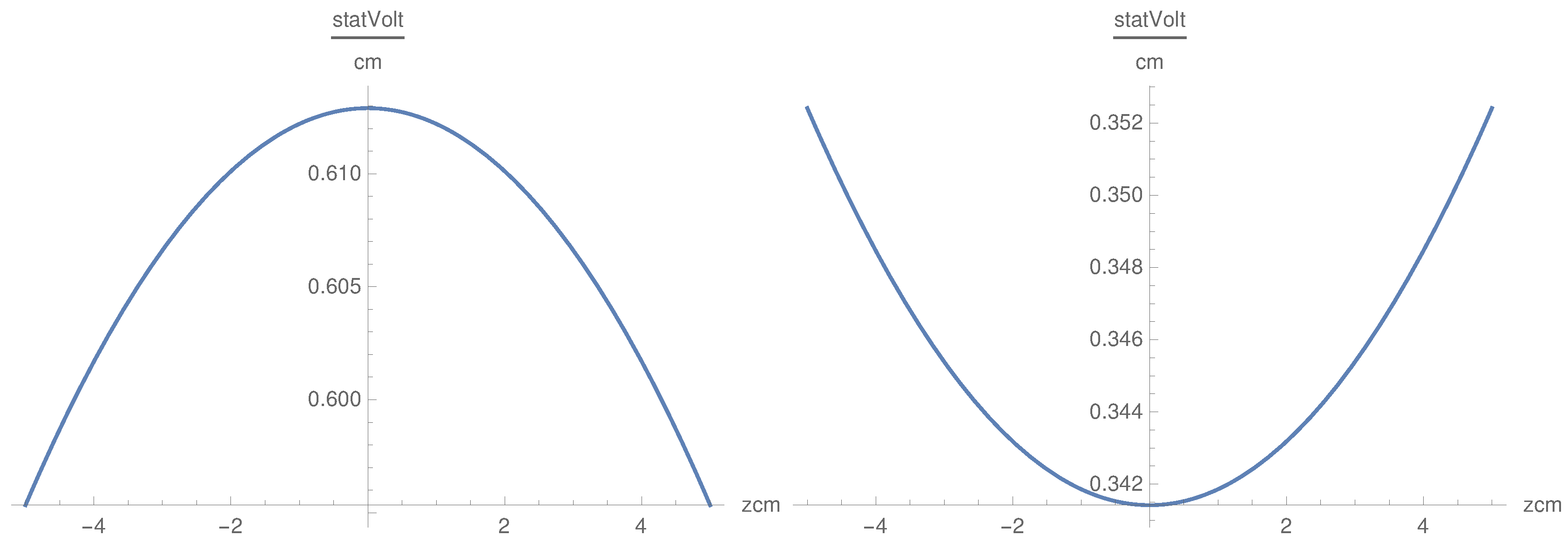
In Figure 4, we show the component $E_y$ as a function of x for $z=1$ cm and with $\omega =1.2$ GHz, which are characteristic frequencies of LH. The $E_y$ component is relatively small with respect to the other components. The curvature of $E_y(x,\omega )$ does not depend on the frequency as shown in Figure 4.

The behavior of $E_y(x,z)$ as a function of z for fixed x is different as there is a maximum for $z=0$ cm. Further, $E_y$ is symmetric in z, the dependence on $\omega$ is not critical, and the shape of the curve remains the same for all values in $\omega \in (1,2)$ GHz. An example of the same is shown in Figure 5.

4.2. $E_z$ Component

We make the inverse Laplace transform and the inverse Fourier transform of

$$E_z=-\frac{s(2k^2-S)}{k^2{s}^2-(s^2+P)(k^2-S)}.$$

(20)

Thus, the inverse Laplace transform is

$$E_z(x,k)=-\frac{(e^{\sqrt{P/S}x\sqrt{k^2-S}}-e^{-\sqrt{P/S}x\sqrt{k^2-S}})(2k^2-S)}{S}.$$

(21)

We then apply the saddle-point method for estimating this integral and expand it with respect to the small parameter ${\lambda }^{-1}=S/\left|P\right|$, as shown in the Appendix. Thus, we get the expression

$$E_z(x,z)=e^{z^2\sqrt{S}/x\lambda }sin\left(x\lambda \sqrt{S}\right)(1+2z^2/\left({\lambda }^2{x}^2\right))S^{1/4}{\left(\lambda x\right)}^{-1/2}.$$

(22)

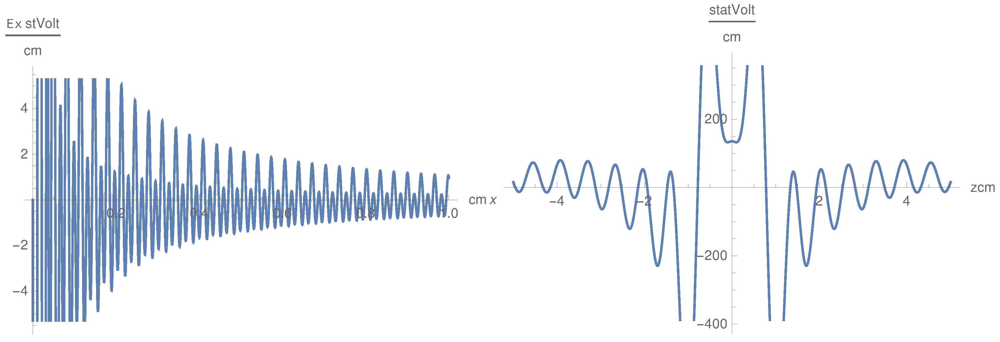
In this case, we get oscillating behavior in the x direction. The dependence on x is oscillatory with oscillations symmetric in z (Figure 6). $E_z(x,z)$ is a convex symmetric function of z as the convexity being modulated by the $sin\left(x\lambda \sqrt{S}\right)$ term (Figure 7). $E_z$, as a function of x, is defined in the interval $(0,10)$ cm, which is different from the behavior of $E_y$. Nevertheless, this result shows that the $E_z$ component, as well as the $E_x$ component, penetrate the plasma with oscillations, which corresponds to the physical situation. The singularity in x at the origin is smoothed by inserting a small positive value in the denominator in the cases of $E_x$ and $E_z$.

4.3. $E_x$ Component

Making the inverse Laplace transform of

$$E_x=-\frac{ik(s^2+P)}{k^2{s}^2-(s^2+P)(k^2-S)},$$

(23)

we obtain

$$E_x(x,k)=\frac{1}{2\sqrt{k^2-S}{S}^{3/2}}(e^{\sqrt{P/S}x\sqrt{k^2-S}}-e^{-\sqrt{P/S}x\sqrt{k^2-S}}).$$

(24)

This expression is similar to that of $E_z(x,k)$, with the only difference being in the denominator. As the final estimate has similar properties and form and the calculations are analogous to those made for $E_z(x,z)$, we have not shown them. Thus,

$$E_x(x,k)=sin\left(\sqrt{\frac{S}{\lambda (x+0.001)}}(z^2+{\lambda }^2{x}^2)\right){\left(\lambda S\right)}^{1/4}/\sqrt{x+0.001},$$

(25)

where $E_x$ shows oscillations in x ( Figure 8) with increasing frequency and has a convex behavior in z with convexity depending on x (Figure 9).

5. Validation

For comparison with the theory and experiments of LHWs, we assume that the electric fields do not depend on the y coordinate and we neglect the $E_y$ component. In the previous theory, this fact holds with a good approximation. The former hypothesis corresponds to LH wave launch structure, which is uniform in the y direction. The assumption of symmetry in the y direction is a reasonable approximation when dealing with LHW coupling using a phased waveguide array [10]. Near the launching structure $x=0$, the electric field has to be directed along the magnetic field line to couple the slow branch corresponding to LH modes. Polarization along the y axis produces a different wave branch, namely the fast wave, which is characterized by a larger phase velocity than the LH slow wave. We have demonstrated that the y component of the electric field is also negligible for $x>0$ cm. The assumptions of this model are the same as the ones used in the previous sections, including that the first derivative of the $E_z$ component is zero statV/cm for $x=0$ cm.

Performing the Laplace–Fourier transform, we obtain the following system:

$$\begin{array}{c}\hfill \left(\begin{array}{cc}{k}^2-S& iks\\ iks& 0& -s^2-P\end{array}\right)\times \left(\begin{array}{c}{E}_x\\ E_z\end{array}\right)\end{array}$$

(26)

$$\begin{array}{c}\hfill =E_z(0,k)\left(\begin{array}{c}ik\\ -s\end{array}\right),\end{array}$$

(27)

where $S,P$ are short symbols for $(S,P){\omega }^2/c^2$ as stated in the first part of this paper and $E_z(0,k)$ is the Fourier transform of $E_z(0,z)$. We assume that $E_z(0,k)$ is zero for $\left|k\right|>>\omega \sqrt{S}/c=k_0$ and zero for $\left|k\right|<k_0$ and that $E_0$ has a constant value. This means that we assume that the launching structure is sufficiently small in the direction of the magnetic field, with a largest characteristic length of d cm, such that a flat spectrum in wavenumber k is produced with minimum absolute wave number $k_1=2\pi /d>>k_0$. We also assume that the launching structure is characterized by a minimum characteristic length $\delta$ cm such that the spectrum in the wavenumber k has a maximum absolute value $k_2=2\pi /\delta$. Usual values for these constants are $E_0=50$ statV/cm, $k_1=1$ cm${}^{-1}$, and $k_2=2$ cm${}^{-1}$. So, the spectrum is given by the constant $E_0$ in the interval $I=(-k_2,-k_1)\cup (k_1,k_2)$.

Making the inverse Laplace transform and inverse Fourier transform, we get

$$\left\{\begin{array}{c}{E}_x(x,z)=\alpha \left(\omega \right){\int }_{k_1}^{k_2}dkcoskzk\frac{sin\alpha \left(\omega \right)\sqrt{k^2-S}x}{\sqrt{k^2-S}},\hfill \\ E_z(x,z)=\alpha {\left(\omega \right)}^2{\int }_{k_1}^{k_2}dkcoskzcos\left(\alpha \left(\omega \right)x\sqrt{k^2-S}\right),\hfill \end{array}\right.$$

(28)

where $\alpha \left(\omega \right)=\sqrt{\frac{\left|P\right|}{S}}$. The integral in k cannot be made using the saddle-point method because it is computed in a finite interval, therefore it has been computed numerically. These formulas coincide with those of the usual theory of LHWs launched by a small antenna. Thus, the general theory is in agreement with the results of the LHWs for the cold plasma at the boundary of the tokamak. We give the graphs of the components in Figure 10 and Figure 11.

We remark that there is strong oscillatory behavior in the x variable for both the $E_x$ and $E_z$ components, while the oscillations have high frequency only for the case of the $E_x$ component in the general theory. The difference is also remarkable for the dependence on z. In the case of the previous theory, we integrated over all the possible values of k, while in this case, the integration is on a finite interval of k and the effect of the finite interval creates oscillations. An experiment for verifying the discrepancies among these two theories would be the study of parametric instabilities [1,2].

6. Conclusions

We formulated a system of Maxwell equations for a magnetized cold plasma, which simulate the physical process of a point-like source localized in the origin $(0,0,0)$ cm and a plasma located in the $x\ge 0$ cm half-space. This source was considered to be the antenna situated at the plane $x=0$ cm generating the electric field at the plane $x=0$ cm with components ${\mathbf{E}}_{\mathbf{0}}\delta \left(y\right)\delta \left(z\right)$ with ${\mathbf{E}}_{\mathbf{0}}=(0,1,1)$ statV/cm. This special form of the vector ${\mathbf{E}}_{\mathbf{0}}$ has been determined to look for physical solutions of the Maxwell equations. Upon changing this condition, one obtains unstable unphysical solutions. The field generated by the antenna was computed in the entirety of the plasma region $x\ge 0$ cm. We also assumed that the magnetic field was ${10}^9$ G and was parallel to the z axis. We chose a given set of plasma frequencies and cyclotron frequencies.

The problem was then to understand how lower hybrid waves (LHWs) penetrate the plasma. We considered frequencies between ${10}^9$–2 $\times {10}^9$ Hz or waves used for heating and diagnostics in tokamak plasma. We made some assumptions which allowed us to find an analytic solution of the problem; we studied the propagation of the wave only in the $(x,z)$ plane and neglected the D coefficient of Stix. Our wave vector is not a usual one $(k_x,k_y,k_z)$ because we made the Laplace transform in the x variable and the Fourier transform in the $(y,z)$. So, the impulses are $(s,k_y,k_z)$, with s being the substitute for $k_x$. Furthermore, $k_y$ was set to zero. We made a list of all of the assumptions made in Section 3. The result was obtained using the saddle-point technique combined with the $1/\lambda$ expansion, with $\lambda$ as a large parameter $\lambda =\sqrt{\left|P\right|/S}$, and with P and S as Stix’s parameters. This choice allowed us to find a solution with physical meaning.

The validation of the theory was performed while generalizing the model to the case of a local antenna located at the boundary of the tokamak using the cold plasma approximation and the hypothesis of constant density and temperature. The analytic formula in this case coincides with those of the theory of the LHWs in the case of the local antenna, but the numeric results are quite different because we used an exact procedure for evaluating the inverse Fourier transform. This consisted of the numeric evaluation of the Fourier integral with high precision, while the calculations in the usual theory were done using some approximation. An experiment for checking our theory would involve measuring the parametric instabilities. This can be executed in the continuation of this work.

References

- Liu, C.S.; Tripathi, V.K. Tripathi, Parametric instabilities in a magnetized plasma. Phys. Rep. 1986, 130, 143–216. [Google Scholar] [CrossRef]
- Porkolab, M.; Bernabei, S.; Hooke, W.M.; Motley, R.W.; Nagashima, T. Motley Observation of parametric instabilities in Lower-Hybrid Radio-Frequency heating of Tokamaks. Phys. Rev. Lett. 1977, 38, 230. [Google Scholar] [CrossRef]
- Babich, V.M.; Buldyrev, V.S. Methods in Short-Wave-length Diffraction Theory; Alpha Science International Ltd.: Oxford, UK, 2009. [Google Scholar]
- Maslov, V.P.; Fedoryk, M.V. Semiclassical Approximation in Quantum Mechanics; D. Reidel Publishing Company: Dordrecht, The Netherlands, 1981. [Google Scholar]
- Dobrokhotov, S.Y.; Cardinali, A.; Klevin, A.I.; Tirozzi, B. Maslov complex germ and high-frequency Gaussian beams for cold plasma in a toroidal domain. Dokl. Math. 2016, 94, 480. [Google Scholar] [CrossRef]
- Anikin, A.; Dobrokhotov, S.Y.; Klevin, A.; Tirozzi, B. Gaussian packets and beams with focal points in vector problems of plasma physics. Theor. Math. Phys. 2018, 196, 1059. [Google Scholar] [CrossRef]
- Cardinali, A.; Dobrokhotov, S.Y.; Klevin, A.; Tirozzi, B. Gaussian beams for a linearized cold plasma confined in a torus. J. Instrum. 2016, 11, C04016. [Google Scholar] [CrossRef]
- Fedoryk, M.V. Saddle Point Method, Encyclopedia of Mathematics; EMS Press: Berlin, Germany, 2001. [Google Scholar]
- Stix, T.H. Plasma Waves; AIP: New York, NY, USA, 1999. [Google Scholar]
- Brambilla, M. Low-wave launching at the lower hybrid frequency using a phased wave guide array. Nucl. Fusion 1976, 16, 47. [Google Scholar] [CrossRef]
Figure 1.
Plot of the Stix function .
Figure 2.
Figure 3.
Figure 4.
as a function of x for cm for GHz (left) and GHz (right).
Figure 5.
as a function of z for cm, GHz.
Figure 6.
as a function of x for some values of z and : Hz and cm (left), and cm and Hz (right).
Figure 7.
as a function of z for some values of x and : Hz and cm (left), and cm and Hz (right).
Figure 8.
as a function of x for some values of z and : Hz and cm (left), and Hz and cm (right).
Figure 9.
as a function of z for some values of x and : Hz and cm (left), and Hz and cm (right).
Figure 10.
as a function of x for cm, Hz (left), and as a function of z for cm and Hz (right).
Figure 11.
as a function of x for cm and Hz (left), and as a function of z, Hz and cm (right).
Publisher’s Note: MDPI stays neutral with regard to jurisdictional claims in published maps and institutional affiliations. |
© 2020 by the author. Licensee MDPI, Basel, Switzerland. This article is an open access article distributed under the terms and conditions of the Creative Commons Attribution (CC BY) license (http://creativecommons.org/licenses/by/4.0/).
Share and Cite
MDPI and ACS Style
Tirozzi, B. Scattering of Lower Hybrid Waves in a Magnetized Plasma. Physics 2020, 2, 640-653. https://0-doi-org.brum.beds.ac.uk/10.3390/physics2040037
AMA Style
Tirozzi B. Scattering of Lower Hybrid Waves in a Magnetized Plasma. Physics. 2020; 2(4):640-653. https://0-doi-org.brum.beds.ac.uk/10.3390/physics2040037
Chicago/Turabian StyleTirozzi, Brunello. 2020. "Scattering of Lower Hybrid Waves in a Magnetized Plasma" Physics 2, no. 4: 640-653. https://0-doi-org.brum.beds.ac.uk/10.3390/physics2040037