Simulation of Spatial Spread of the COVID-19 Pandemic on the Basis of the Kinetic-Advection Model

1
Dorodnicyn Computing Centre, Federal Research Center “Computer Science and Control” of Russian Academy of Sciences, Vavilova str. 40, 119333 Moscow, Russia
2
Federal State Budget Educational Institution of Higher Education «MIREA—Russian Technological University», 78 Vernadsky Avenue, 119454 Moscow, Russia
*
Author to whom correspondence should be addressed.
Physics 2021, 3(1), 85-102; https://0-doi-org.brum.beds.ac.uk/10.3390/physics3010008
Submission received: 31 December 2020
/
Revised: 5 February 2021
/
Accepted: 12 February 2021
/
Published: 18 February 2021
(This article belongs to the Special Issue Physics Methods in Coronavirus Pandemic Analysis)
Abstract
:A new two-parameter kinetic equation model is proposed to describe the spatial spread of the virus in the current pandemic COVID-19. The migration of infection carriers from certain foci inherent in some countries is considered. The one-dimensional model is applied to three countries: Russia, Italy, and Chile. Both their geographical location and their particular shape stretching in the direction from the centers of infection (Moscow, Lombardy, and Santiago, respectively) make it possible to use such an approximation. The dynamic density of the infected is studied. Two parameters of the model are derived from known data. The first is the value of the average spreading rate associated with the transfer of infected persons in transport vehicles. The second is the frequency of the decrease in numbers of the infected as they move around the country, associated with the arrival of passengers at their destination. An analytical solution is obtained. Simple numerical methods are also used to perform a series of calculations. Calculations us to make some predictions, for example, about the time of recovery in Russia, if the beginning of recovery in Moscow is known.
1. Introduction
The COVID-19 pandemic is a serious challenge not only for medicine, but also for other scientific disciplines including physics and mathematics. Numerous scientific groups worldwide are working on this problem based on different and complex models using high performance computing.
There are many models that aim to describe epidemics. Let us note the well-known susceptible, infectious, and removed individuals (SIR) model and similar ones. In this sense, first, one can mention the original paper [1]. The vast review of a family of the methods is presented in the monograph [2]. Although the basic mechanisms of each phenomenon are different, their effective mathematical description often defines similar constitutive equations and dynamical behaviors framed in the general theory of reaction-diffusion processes [3], see also [4].
The family of SIR-based models describe the changes in the number of susceptible, infectious, and removed individuals over a considerably large period of time. Some more sophisticated models consider the specifics of COVID-19, although they become complicated due to the number of parameters that need calibrating [5]. For an overview see also [6]. Note that, in general, SIR models do not take into account the population density at different points in space. The main difference of our model from SIR-like models is that we intend to describe the spatial spread of the epidemic in time (which SIR models do not) when local infections can be neglected. We study the movement of the wave of infections along the selected direction, but we do not consider the entire time evolution of the epidemic in a given area, since a few weeks after the first infections, it is already determined by local infections.
Our model takes into account population density, which strongly determines the profile of the spatial infection wave. We should mention the model of the spatial propagation of the first wave of the virus in space and time [7]. As proposed in this model, the number of infected individuals is supposed to be proportional to the power of distance of the source of epidemics and the power of the population in a given city. The powers of the values are obtained using freely available data about cases of COVID-19. We also propose a two-parameter model, but these parameters have strict physical meaning: the speed of migration of infected individuals and resistance value that depends on various factors, for instance, the quarantine measures. We show that the exponential decrease of the number of infected individuals is a result of the transport equation, and it depends not only on distance but on the population density.
In [8], the investigation is presented how the number of cases by COVID-19 scale with the population of Brazilian cities. Here, e.g., urban scaling relations of COVID-19 cases, the time dependence of the scaling exponents for COVID-19 cases, and the association between growth rates and city size are shown. However, in that paper, the spatial spread of the epidemy over long distances is not studied. There is some statistical research on how different factors affect the COVID-19 spread (see [9,10,11]). The most relevant to this work is the analysis of spatial factors. However, in those papers, there is no proposition of a deterministic model that describes the spatial propagation of a virus around countries.
Various spatial models of the spread of viruses are known, but they often contain many parameters that require determining their exact mutual correspondence. Simpler models that convey qualitative and quantitative patterns of the distribution would certainly be of interest, both scientific and practical.
Among the factors contributing to the spread of the COVID-19 infection, one can note the current significant speed of vehicles and a large number of social contacts in cities. At the same time, modern information technologies make it possible to quickly track down the spread of the pandemic, as well as collect sufficiently accurate data to construct adequate mathematical models (the resources [12,13,14,15] are used). There are studies devoted to the problems of modeling biological and social processes. Note that in [16,17] a diffusion-type equation is used. On the basis of such methods, various autowave processes were studied, including the spread of infections, see, e.g., [18]. In [19], kinetic transport equations were considered to study the nature of traffic flows. In [20], kinetic equations were used to model some sociohistorical processes including a model of aggression.
It is important that in the dynamical changes of the spatial distribution of COVID-19, two independent factors coincide. One is the advection related to the transport vehicles, the other the counteraction with the outer media. In fact, the latter denotes decreasing the number of passengers coming back to their home. The adequate apparatus is the kinetic equation; the direct methods for this is described in [21]. However, in the present case the equation is quite simple; we suggest a one-dimensional advection-kinetic type model of the spatial movement of infected carriers in Russia, Italy, and Chile. For these countries, the migration of carriers of the virus occurred from the designated centers: Moscow (the spread of the virus eastward from the capital is confirmed), the province of Lombardy, in Italy, and Santiago, Chile, respectively. The use of a one-dimensional model is justified by socio-geographical conditions: the proportion of “length” to “width” is quite large. Lateral invasions of the virus can be ignored. In Russia, the northern areas are sparsely populated, in the south there are deserts and mountains on the borders with other countries. In Italy, from the west and east, the Apennine peninsula is outlined by the Tyrrhenian and Adriatic seas, respectively. In Chile, the Pacific Ocean is to the west, and the high Andes to the east.
The one-dimensional model uses averaging over rather large territories of countries. The map of each country is divided into large bands. For Russia, 7 bands are allocated, for Italy—9, for Chile—4 and 3 (to the north and south of Santiago, respectively). The proposed model is determined by the following parameters: is the average speed of transport coming from the center of infection and σ is the “resistance” to the movement of carriers of the virus by vehicles. In this kinetic-figurative approach we consider the early days of the COVID-19 pandemic in the spring of 2020. This model is close to the models used in [20]. But in the present work it is simpler since it is linear. In contrast to the mentioned work, where background elements that participated in the interaction were eliminated, in our model the background parameters do not change with the advancement of the infected elements in space.
Our model, in general, is a “ballistic-kinetic” rather than a “reaction-diffusion” model. The fundamental difference is that in our approach, the spread of infection is not associated with a gradient in the number of infected. In the known model, the infection moves from an area with a large number of cases to an area with a smaller number, in other words, according to the corresponding diffusion equation. In our method, we consider the spread, which is not directly related to the number of infections, since the spread rate is due to another factor, namely, the average speed of transport (including cars, buses, trains, and airplanes). Thus, the spread of infection can occur from a region with fewer infected people to a region with a large number of infected people, that is, in the direction of the infection gradient. In the situations under consideration, indeed, the initial concentration of diseases, for example, in Moscow, is much higher than in the periphery, but the spreading process cannot be described by diffusion.
Two mechanisms of the infection spread can be defined: a transferential mechanism and a contact one. In our work, the transferential mechanism is studied, that is, infections caused by the migration of infected carriers from the center of infection. The contact mechanism comes in after the relocation of infected carriers from the center, and it is due to the contagion within the regions. The superposition of these two factors gives the sum of all infected. The first phase of the process involves transferential contamination. This phase lays the foundations for the next phase of the infection development associated with local contacts. Contact infections are more pronounced with the introduction of quarantine isolation measures in individual regions. The third phase is associated with the spread of “recovery”, which is determined, in particular, by reaching a maximum of new infections per day for each region. Infected individuals travel by various vehicles. We consider the average speed, which takes into account the speeds of different air-, land-, and water-based vehicles. Another parameter of the suggested model is the value of “resistance” to the movement of virus carriers. The main equation of the model is the inhomogeneous transport equation with a kinetic term on the right-hand side: the decrease in number of carriers is taken into account which is associated with the carriers returning to their places of residence from the center of infection. Quarantine barriers between regions also play a role. Some predictions according to the present model are discussed, namely, the data of the recovery for the whole country, as we know that the velocity of recovery is approximately equal to the velocity of infection.
2. Mathematical Model
Analogously to [20], in order to determine the density of infected passengers disembarking at a certain place at a certain point in time, the following non-uniform transfer equation is applied:
where t is the time, x is the distance, n(t,x) is the density of moving virus carriers in a vehicle, is the speed of a vehicle, and σ—the coefficient of “resistance” to the movement of infected elements mainly due to the landing of passengers in places of residence, it is measured in units of temporal frequency. This is a simple form of the well-known kinetic equation, in which the left-hand side describes the advection of particles, and on the right-hand side the collision process is presented, here we consider the linear case without the gain term. We emphasize that this is not an ordinary diffusion-reaction equation. Here, advection is not the result of a corresponding mass gradient as in the diffusion equation. The speed of movement of passengers (or elements or particles in physical terms) is related to the speed of the vehicle.
The initial condition for the Cauchy problem is:
where H(x) is the Heaviside function. In other words, = 0 for t = 0 and for x > 0. This formulation of the problem means that in the studied area where x > 0 carriers of the virus enter across the border x = 0, which corresponds to the idea of the main permanent source of infection.
Let us use the method of characteristics to solve Equation (1). Let thus:
Comparing this expression with the left-hand part of Equation (1), we see that if , , we get the following ordinary differential equation:
which has an exact solution: . From and , we get that , thus from , we obtain that , where . Thus we get:
In fact, we use standard methods for solving linear partial differential equations, see, e.g., [22]. Assuming n(t,0) = 1 for t > 0, the solution is as follows:
Here, a day is taken as a unit of time, a km is taken as a unit of distance, respectively, the speed is expressed as km/day, “resistance coefficient” (frequency) has the dimension .
We will denote the density of virus carriers that landed at a given point by (t,x). It is clear that this density increases with the decrease of n(t,x), thus we can write:
and, since
taking into account Equation (1), the equation for (t,x) is:
The solution of this equation is given by:
The substitution of Expression (2) and the zero initial condition allows us to an expression for (t,x):
The density of disembarked passengers grows with time as infected new people arrive. It is important to note that the profile of infected passengers in the vehicle n(t, x) with time goes to some definite curve, exponentially decreasing in space. However, the density will constantly increase in time at each spatial point if conditions are not changed. The introduction of an area isolation regime can be an example of such change. In this case, it is necessary to change the boundary conditions.
We also used a simple numerical method to obtain a large number of variants of a solution. We applied the finite difference scheme [23].
In general, σ can be a function of t and x. can also be a dependent quantity, but we assumed it to be constant. One of the options for the dependence of σ on the coordinate can be obtained by taking into account the population density:
where ρ(x) is the linear population density, having dimension 1/km, and is an arbitrary constant of dimension km/day.
Substituting Equation (5) into Equation (2), we obtain the following expression:
A similar substitution into Equation (4) yields
In order to determine the parameter , we fix t in Equation (6) and write it down for two values of x: x = 0, the center of infection spread and x = Δ, the distance to the second band, and approximate the integral by the trapezoid formula:
As noted above, along the selected direction of the spread of infection, the territory of the country is divided into stripes. In open sources there is information on the number of new cases of infection and recovery for each day by region [12,13,14,15]. To approximate these data in the selected bands, we summarized the values in the regions included in the band with the corresponding weights. The weight was calculated as the ratio of the population density in the region to the sum of the densities for all the regions included in the strip. Let be the number of new infections per day for a strip. For the i-th region, the number of new infections is known. Suppose that the strip includes N regions. We have a set of values ,…,. Len ,…, be the population density in the regions included in the strip. Then the parameter a can be represented as a weighted sum:
Russia, Italy, and Chile were selected to apply the model. In these countries, the spread of infection occurred mainly in one direction from a dedicated center. This was facilitated by the uniqueness of the situation and the geographical characteristics of the countries. The most important sources of the epidemic were associated with the metropolitan centers of the countries (Moscow—the capital of Russia, Milan—the capital of Lombardy in Italy, Santiago—the capital of Chile), which were visited by tourists or citizens of this country, returning from other countries in which the epidemic had already begun. In Russia, citizens returning from abroad go through Moscow to the east to their places of residence. The geographical extent of the country allows us to consider a one-dimensional equation.
3. Simulation of the Spread of the Epidemic in Italy
In Italy, there was a spread from the Lombardy region to the southeast along the narrow Apennine peninsula. The country’s territory was divided into 9 bands (Table 1), in which the values for a number of infected people were found as weighted sums for the regions included in the band. The population density is shown in Figure 1 where the distribution in the bands is taken into account.
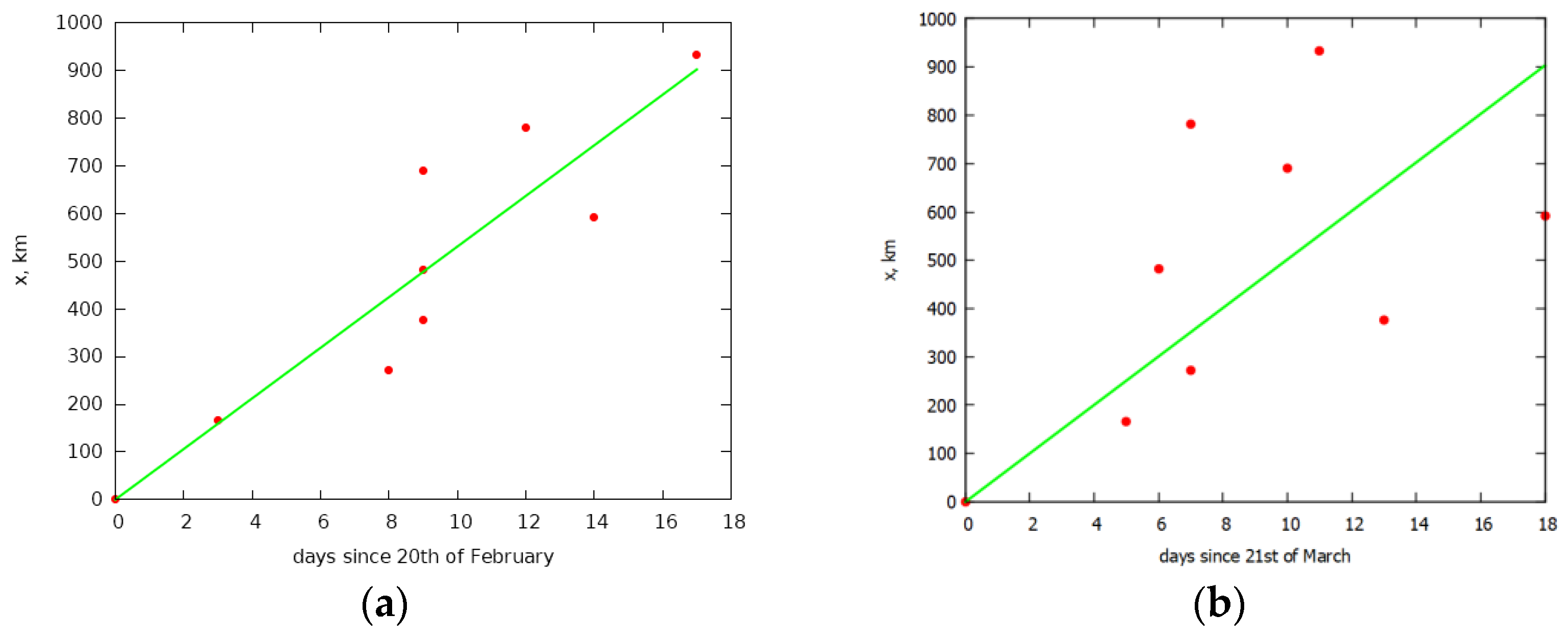
The parameter, which determines the rate of spread of infected elements, can be estimated from the data on the first infections in each band. We used the first day, on which there were at least 5 cases. Having constructed the points corresponding to these days, using the least squares method, we will construct a straight line passing through the point corresponding to the center of infection (Lombardy). is equal to the tangent of the slope of this straight line in Figure 2a.
The parameter, which determines the rate of spread of infected elements, can be estimated from the data on the first infections in each band. We used the first day, on which there were at least 5 cases. 5 is an arbitrary number, but the higher the number the more it is affected by the contact mechanism of the virus spread, and the lower the number, the more it is affected by the statistical error. Having constructed the points corresponding to these days, using the least squares method, we will construct a straight line passing through the point corresponding to the center of infection (Lombardy). The additional condition is that the line passes through the origin point which corresponds to the day when there were at least 5 cases in the first band. is equal to the tangent of the slope of this straight line in Figure 2a.
Although the average speed of vehicles can be obtained through other methods or by using a higher order polynomial for the least squares method, the method described here, despite its simplicity, can yield some prediction power which is shown in the results section of this paper.
The values from Figure 2b were used to determine the speed of recovery. The way it was done is explained later in the text.
For Italy, we get the speed: = 53 km/d. Using Equation (7), we obtain = 0.0012 km/day.
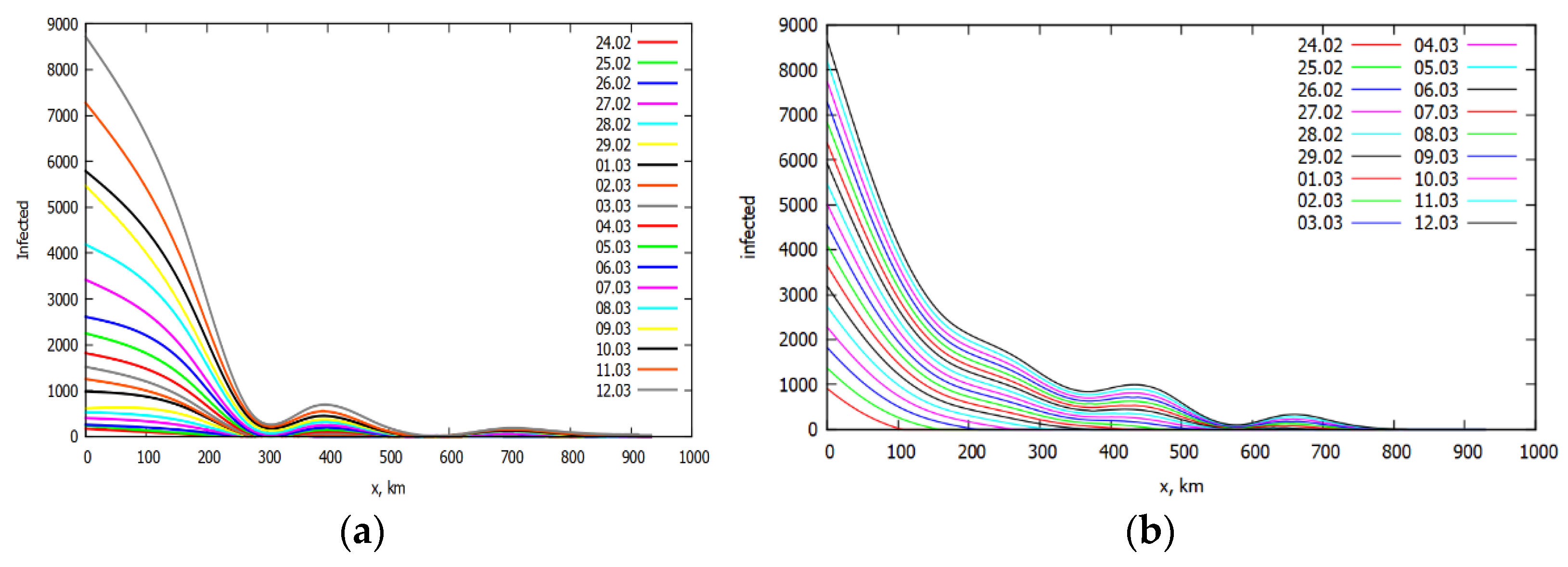
A comparison of the numerical solution for with real data for Italy at the initial stage of infection is shown in Figure 3. The graphs show that the nature of the real and theoretical distributions is similar to each other, but the values of the real data are higher than the theoretical ones. This phenomenon is observed due to the larger population in the second band, which is due to the large number of Italian regions included in the second band.
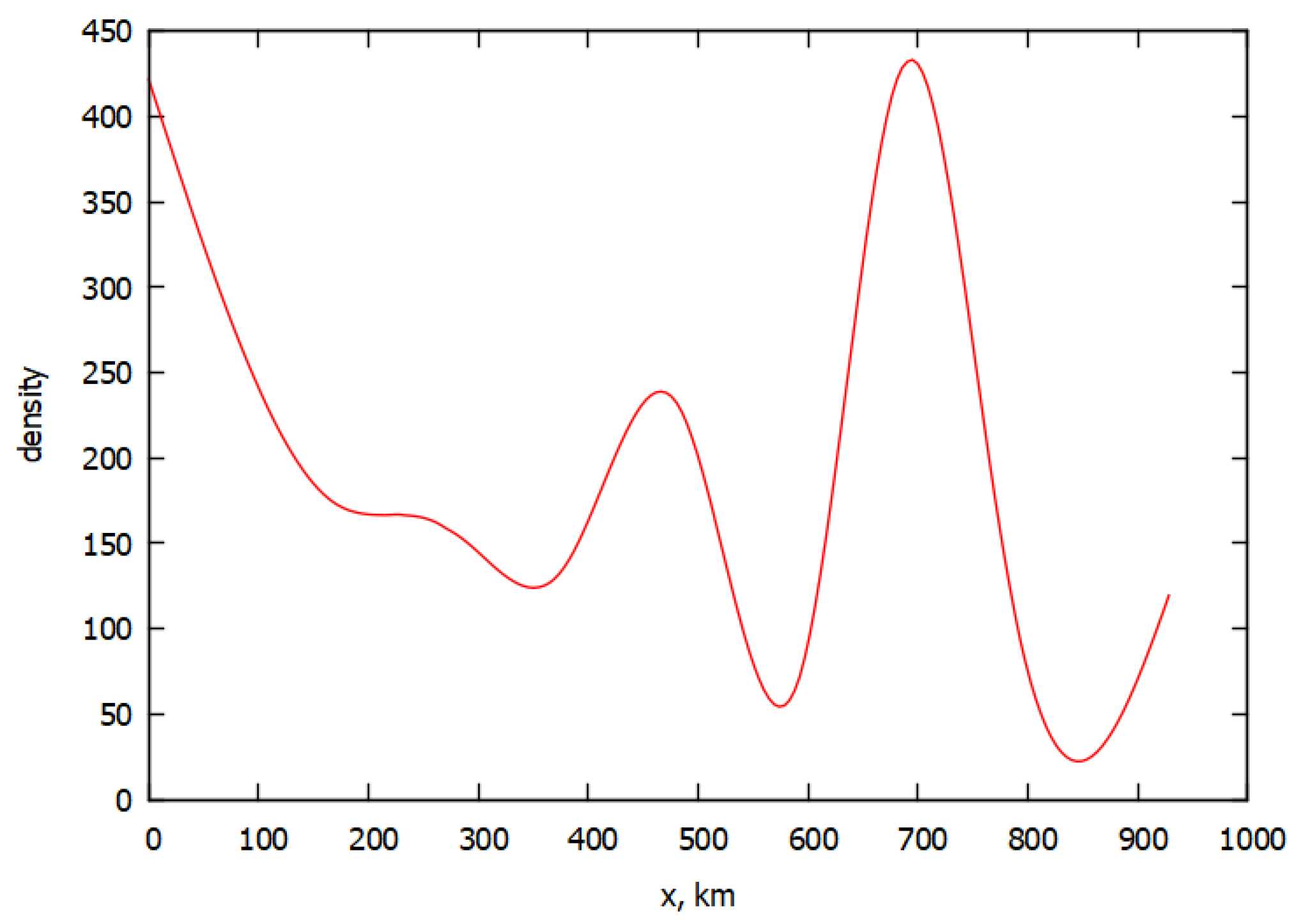
Here is a consideration when comparing population density and distribution in Italy, see Figure 1 and Figure 3. There is a certain correlation between extrema on the two graphs. Moreover, the second maximum in Figure 3 is small due to a decrease in the number of moving infected. It is important that these maximums on the real distribution graph and the calculation graph correspond approximately to each other. There is a characteristic detail in both graphs, namely, the data maxima are shifted to the left compared to the maxima on the population density graph, which can be explained by the peculiarity of the decrease in the number of infected passengers. It can be assumed that the maximum of infected is associated with the maximum of the derivative of the density. The increase in population density is associated with the appearance of cities in these places on the map and, consequently, with the train stations, bus stations, and airports on the border of these cities. On the other hand, quarantine barriers can also play a role.
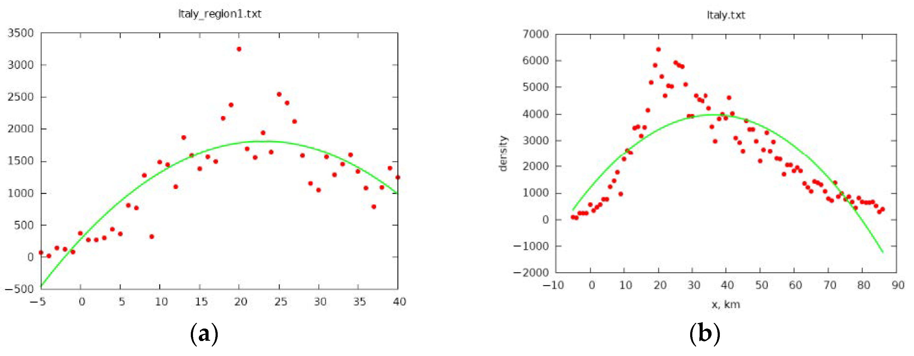
We define the onset of recovery for the selected band as reaching the maximum infections per day. The least squares method was used with an approximation using a second order polynomial. For each parabola, a maximum was determined, which correlated with the date of the beginning of recovery for this band. The data on the maximum infections per day for each band is shown in Figure 4 (only some bands are shown for brevity). In these plots, 0 on the x-axis is 1 March.
The rate of recovery was determined in the same way as the rate of infection (using the method of least squares with a linear approximation), see Figure 2b, the amounted to 50 km/d. According to the schedule of the spread of recovery, one can predict the approximate time of the beginning of recovery for Italy as a whole, namely the date when the line of distribution of recovery passes the point corresponding to about half of the population of the country. In Figure 2b, the origin on the abscissa corresponds to the beginning of recovery (reaching the maximum infections) in Lombardy. Due to the heterogeneity of the density distribution (see Figure 1), approximately half of the population of Italy corresponds to a territory up to a distance of 600 km from Lombardy. This point in Figure 2b corresponds to 2 April. As predicted from Figure 2b, the time of the beginning of recovery for the whole of Italy is corresponding to the beginning of recovery according to Figure 4, which shows that the maximums of infection are reached in the first week of April.
The rates of infection and recovery were approximately the same. This conclusion is consistent with the assumption that the conditions for the course of the disease were akin to each other in different areas, which is ensured by strict quarantine isolation of each area.
4. Simulation of the Spread of the Epidemic in Chile
In Chile, the main source of the spread of the virus was the capital of the country, Santiago, located approximately in the middle of the extended country. Four bands were allocated north of Santiago and 3 bands south of the capital. The data for Chile were aver-aged for each band by the regions included in it the same way as for Italy.
In the simulation, two different directions are considered independent of each other, that is, it is assumed that the number of infected passengers who left, for example, in the direction of the north, and then turned south, will be negligible compared to the total number of passengers. The bands in the north direction are shown in Table 2. The bands in the south direction are shown in Table 3.
Further to the south of Los Lagos, there are two more regions. These regions are not taken into account in this work, because of low population density in these regions so the statistics on coronavirus are comparable to the error in other regions.
The population density is shown in Figure 5. In the graphs hereinafter, Santiago is not considered (reference point x = 0), since the population density in this city is an order of magnitude higher than in other bands. Therefore, the density is taken into account from the first band in each direction—they are located at a distance of 50 km to the north and south of Santiago. From Figure 5 it can be seen that to the north, the population density from the first strip begins to decrease and then rises, and in the south, the density initially increases slightly, and then decreases.
The parameter values obtained for Chile by the same methods as for Italy have the following values: = 44 km/d, = 0.0026 km/day for the north and = 97 km/d, = 0.0065 km/day for the south. The appropriate graphs for southern Chile are shown in Figure 6 (for the north they are similar).
A comparison of the numerical solution for with real data at the initial stage of infection for southern Chile is shown in Figure 7. Figure 7a,b have some similarities, despite the rather uneven growth of real data.
The rates of recovery were found the same way as for Italy (Figure 8). The rates of recovery: = 23 km/d to the north of Santiago and = 96 km/d to the south. A mismatch in the rate of recovery of the rate of infection in the north may indicate some inaccuracy in the data or data insufficiency. Again, in Figure 8 only data for the south is shown and only plots for one band and all bands to the south of Santiago are shown for brevity.
In Figure 6b the abscissa origin corresponds to the beginning of recovery (reaching the maximum infection) in Santiago. Despite different distributions of population density to the north and to the south of Santiago, about half of the population in each direction corresponds to a distance of 400 km from the capital (see Figure 5). This point in Figure 6b corresponds to July 7 in the south. Predicted from Figure 6b, the prediction for the south turned out to be less accurate than it was for Italy.
5. Simulation of the Spread of the Epidemic in Russia
In the direction to the east, the territory of Russia on the map was divided into 7 bands, as given in Table 4. The population density by bands is shown in Figure 9a. The source code for computing the weighted values of infected individuals and for computing is available in Appendix A.
The parameters obtained for Russia by the same methods as for Italy have the following values: = 87 km/d, = km/day. The graph according to which the speed was found is shown in Figure 10a. The speed turned out to be higher than the same parameter in Italy due to a much greater length of the country, hence the average speed of vehicles is higher. For example, it can be assumed that airplanes (the fastest mode of transport) are used for domestic traffic in Russia more often than in Italy, which as a result gives a higher travel speed in Russia.
Numerical calculations for the time after two weeks of infection confirm qualitatively the development of the infection, and, naturally, lower values compared to the real data. Here the second—the contact factor—plays the main role. It is assumed that the quarantine conditions are strictly fulfilled, so the transfer of infection does not matter anymore.
In Figure 9b, it can be seen that the real values for two consecutive dates begin to grow faster than the calculated ones due to infections in the field.
The rate of recovery was found the same way as for Italy and amounted to 52 km/day.
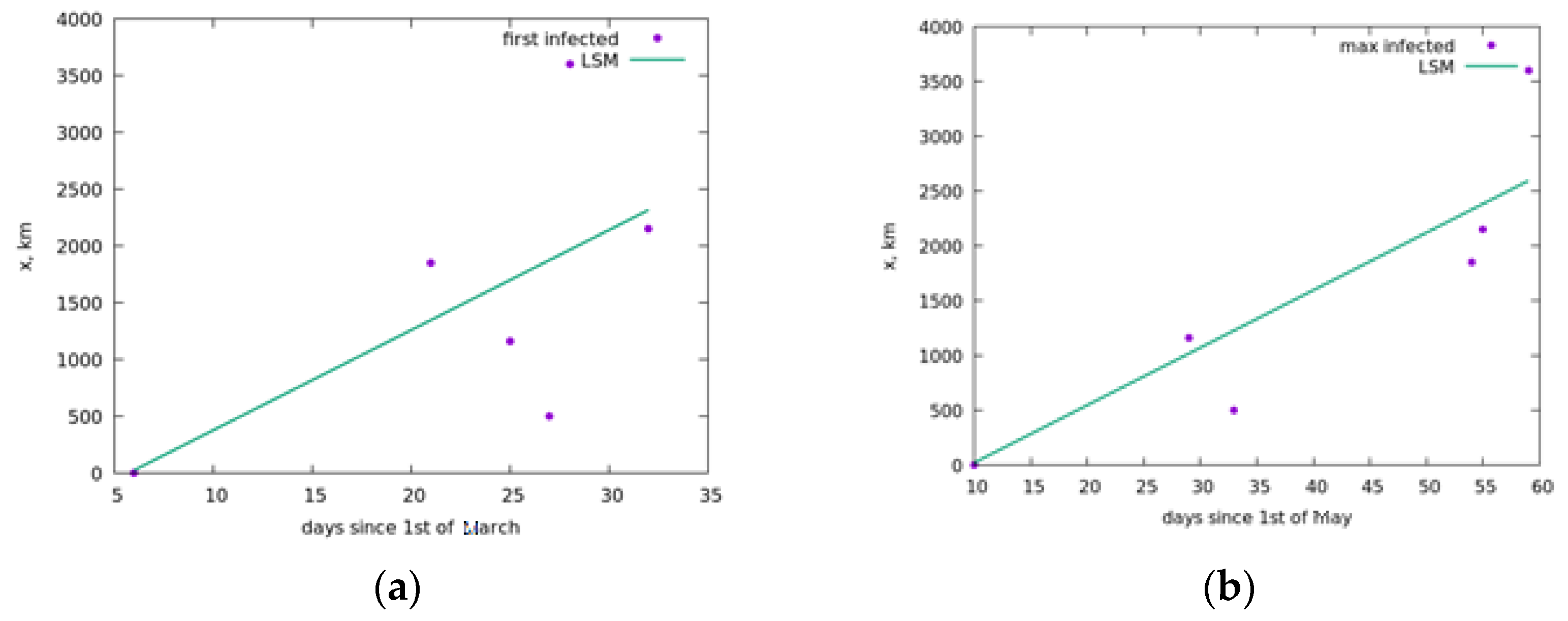
In Figure 10b, the x origin corresponds to the beginning of recovery (reaching the maximum infection rate) in Moscow. About half of the Russian population corresponds to a distance of 1000 km from Moscow (see Figure 9a). This point in Figure 10b corresponds to May 30. As predicted from Figure 10b, the time of the beginning of recovery for the whole of Russia is corresponding to the beginning of recovery according to Figure 11b, which shows that the maximum of daily infected reached by the beginning of June.
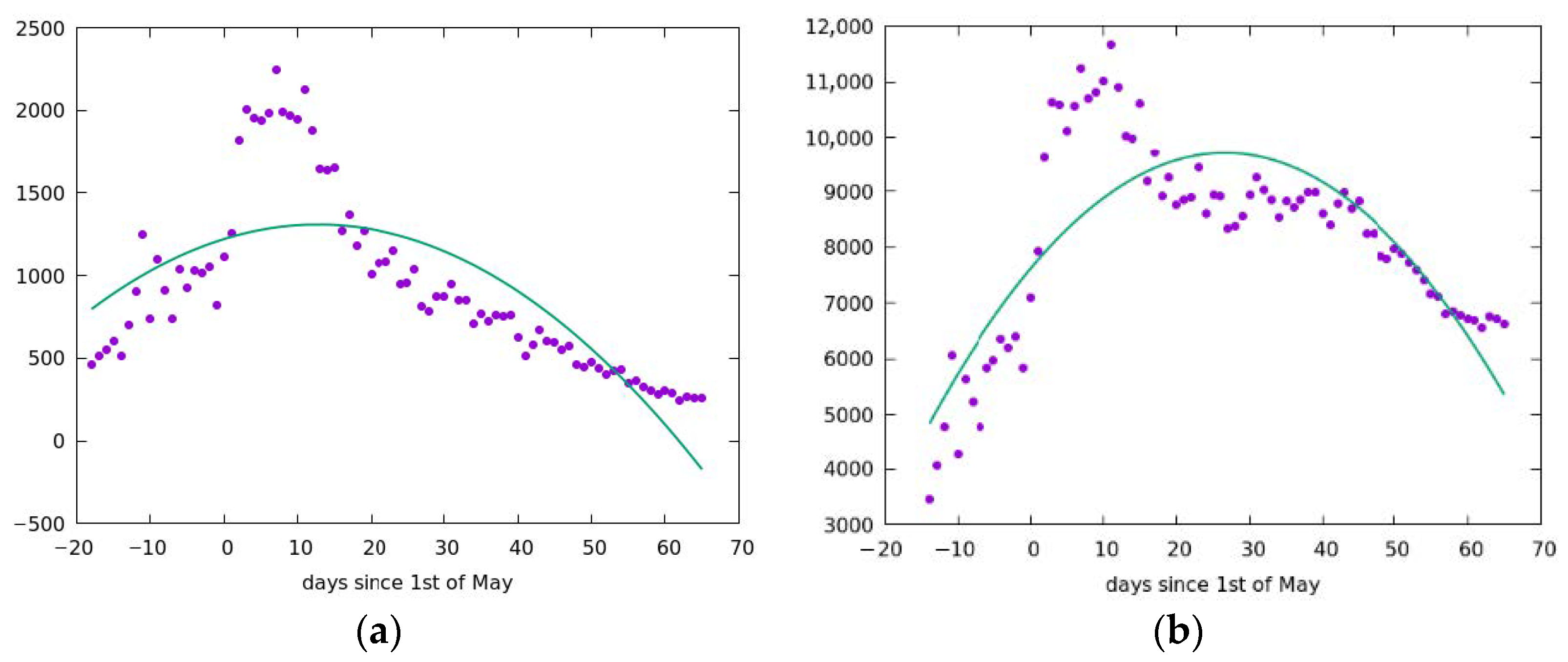
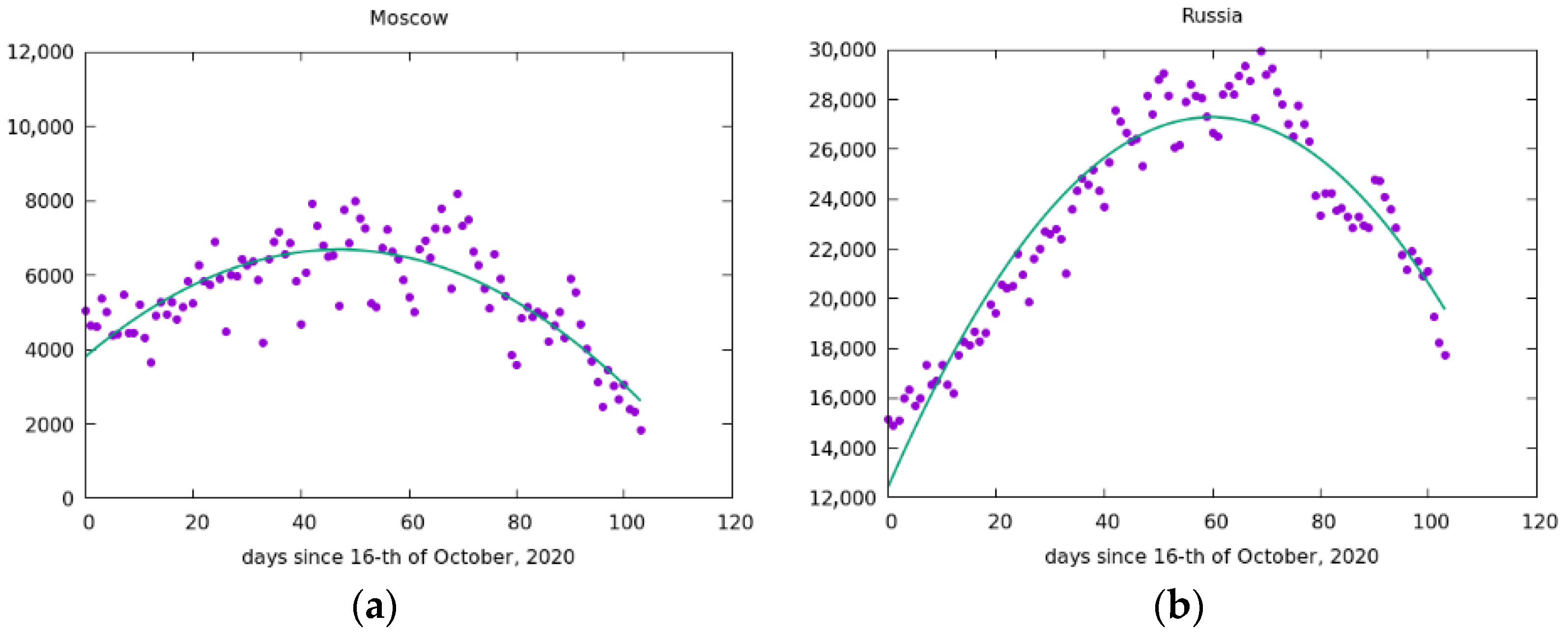
Currently, a new wave of the pandemic has emerged, and such clear conditions for the development and spread of COVID-19 are no longer observed. The autumn wave of the pandemic is more complex, which was facilitated by many factors, in particular, there was no such strict isolation as in the spring. Nevertheless, it can be assumed that Moscow was the main center for the spread of the virus to the east. Therefore, the maximum infection in Moscow can be reached about three weeks earlier than in the whole of Russia (see Figure 12). Our prediction concerning the difference between the mentioned maximum in Moscow and in Russia as whole: in Moscow on around 10 December and we expect that the maximum in Russia will be around 31 December.
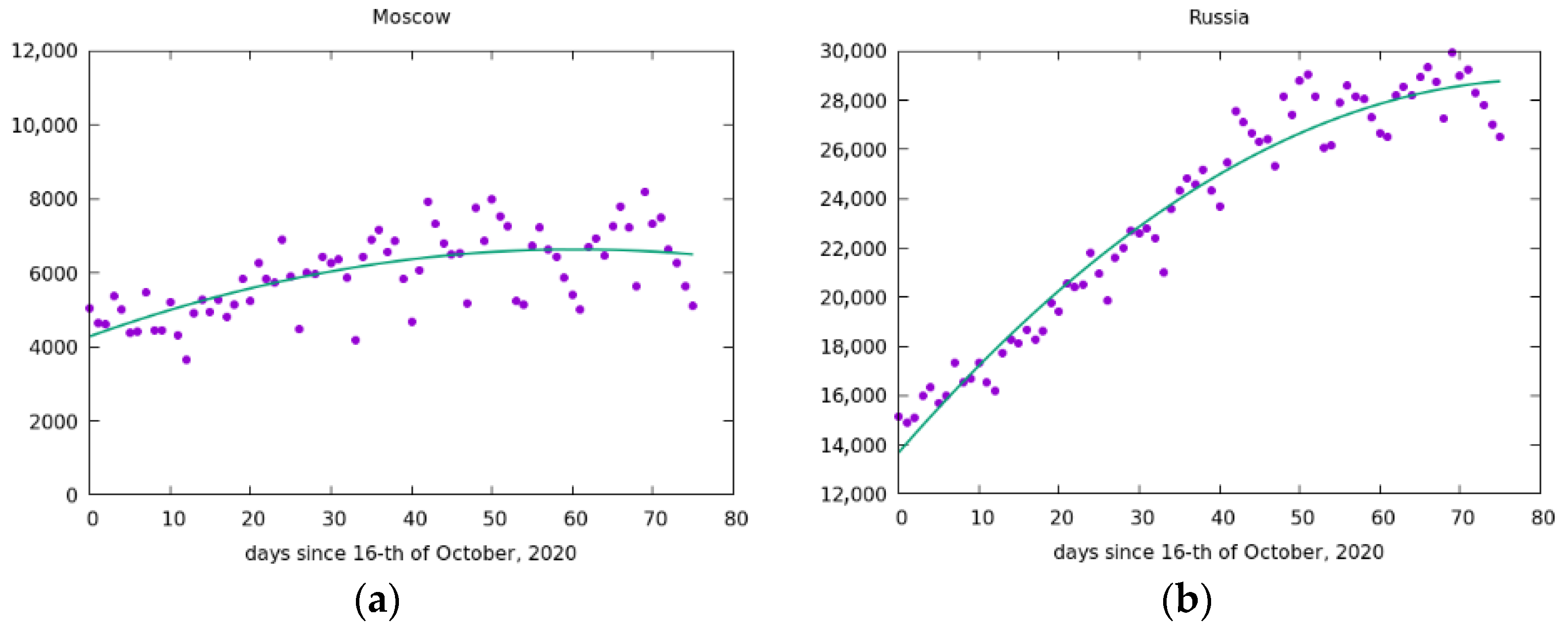
In Figure 13 some additional data known in January 2021 was added to check the prediction. The maximums of parabolas moved by about 2 weeks to earlier dates (this is a consequence of the method of the least square root) but the distance between maximum in Moscow and maximum in Russia stayed approximately the same.
6. Conclusions
This paper presents a model capable of replicating the spread of coronavirus (COVID-19) in some countries with a distinct focus on the disease. A two-parameter kinetic one-dimensional model of the spatial spread of coronavirus infection was proposed using the example of three countries: Russia, Italy, and Chile. An essential assumption is related to introducing strict quarantine starting from a certain time and fulfilling it for a sufficiently long period. It was assumed that, before the start of quarantine, the transmission of infection took place practically only due to returning passengers from the mentioned centers, the way it happened in three countries under consideration. A comparison of the calculations with real data showed good agreement for the first weeks of the transmission of infection.
The process of recovery is in a sense “symmetrical” to the process of infection: recovery begins earlier in those places where the infection occurred earlier. Thus, the results obtained also have predictive capabilities. By contrast, the second wave of the pandemic does not fit into such a clear picture. The autumn wave is more complex, which was facilitated by many factors (in particular, there was no such strict isolation as in spring 2020). Nevertheless, it can be assumed that, during the second wave, Moscow was again the main center for the spread of the virus to the east of Russia. Therefore, the maximum infection in Moscow can be reached about two or three weeks earlier than in the whole of Russia. Our important forecast points to a difference between the indicated maximum in Moscow and Russia as a whole: in Moscow on around December 10, and we expect the maximum in Russia to be closer to the end of December. This prediction was confirmed taking into account new data from January.
Further work can be done with this model or its modifications. For example, it is possible to consider the migration of virus carriers returning through Khabarovsk, which is located, on the Far East of Russia, in addition to Moscow. This would put additional boundary conditions and thus alter the resulting equation. A similar modification of the problem for Italy would make sense not on the right (southeastern) border, but in the middle of the country for Rome and Naples.
The study of the more detail spread of the epidemy needs using “2D maps”, i.e., using two-dimensional form of the equation. From Moscow the waves of the epidemic spread along radial rays. In the simplest case of spreading the wave from Moscow to the east one can consider a central symmetry, the radius of the circle will be the only independent variable.
Strictly speaking, there was the other important center of infection in Russia, namely, in St. Petersburg, to the west of Moscow, but the spread of epidemics westward from the capital was not examined. The area between Saint Petersburg and Moscow can be considered as a two-dimensional region with an advection-kinetic equation without any symmetry. The model in a two-dimensional form with many centers of infection requires more complex numerical calculations (it is a significant fact that the primary source of infection appeared in St. Petersburg earlier than in Moscow).
Author Contributions
Conceptualization, V.V.A.; data curation, A.V.S. and A.D.Y.; formal analysis, V.V.A., A.V.S. and A.D.Y.; funding acquisition, V.V.A. and A.V.S.; methodology, V.V.A.; software, A.V.S. and A.D.Y.; supervision, V.V.A.; visualization, A.V.S. and A.D.Y.; writing—original draft, A.V.S.; writing—review & editing, V.V.A., A.V.S. and A.D.Y. All authors have read and agreed to the published version of the manuscript.
Funding
The authors are grateful to the Russian Foundation for Basic Research for financial support: grants 18-01-00899 and 18-07-01500.
Conflicts of Interest
The authors declare no conflict of interest.
Appendix A. C++ Code for Computing for Russia
#include <iostream>
#include <sstream>
#include <vector>
#include <cmath>
#include <cassert>
#include “spline.h”
using namespace std;
const double tau = 0.01;
const double h = 0.02;
const double xmax = 6.5;//Moscow -- Anadir: 6212 km
const size_t x_size = xmax/h + 1;
double u = 0.087;//thousands of km
double T = 0;
double sigma1 = 0;
vector<double> dens_x {0, 0.5, .7, 1.16, 1.85, 2.150, 2.5, 3.6, 6};
vector<double> dens_y {434.63, 28.77, 16, 14.1, 11.26, 4.53, 3, 1.67, 3.08};
tk::spline n1;
double sigma(double x) { return sigma1 * n1(x); }
int main(int argc, char** argv)
{
double scale = 1;
for(int i = 1; i < argc; ++i)
{
string opt(argv[i]);
auto index = opt.find(‘=‘);
if(index != string::npos) opt[index] = ‘ ‘;
stringstream sopt(opt);
sopt >> opt;
if(opt == “t”) sopt >> T;
if(opt == “u”) sopt >> u;
if(opt == “sigma”) sopt >> sigma1;
if(opt == “scale”) sopt >> scale;
}
n1.set_points(dens_x, dens_y);
vector<double> n(x_size);
vector<double> nm(x_size);
vector<double> next(x_size);
n [0] = 1;
for(double t = tau; t <= T; t += tau)
{
next[0 ] = 1;
nm[0]+=tau*sigma(0)*n[0];
for(size_t i = 1; i < x_size; ++i)
{
next[i] = n[i]*(1 - u*tau/h - tau*sigma(i*h)) + n[i-1]*u*tau/h;
nm[i]+=tau*sigma(i*h)*n[i];
}
n.swap(next);
}
//printing results for each region
cout << 0 << ‘ ‘ << scale*nm[0] << endl;
cout << 500 << ‘ ‘ << scale*nm[0.5/h] << endl;
cout << 1160 << ‘ ‘ << scale*nm[1.160/h] << endl;
cout << 1850 << ‘ ‘ << scale*nm[1.850/h] << endl;
cout << 2150 << ‘ ‘ << scale*nm[2.150/h] << endl;
cout << 3600 << ‘ ‘ << scale*nm[3.600/h] << endl;
}
Source code in Python for generating regions using weighted sums for Russia.
N = 22 #number of data columns
def app(out, fname, w):
print(“Append: “, fname, w)
global N
f = open(fname, ‘r’)
lines = f.readlines()
for i in range(0, len(lines)):
line = lines[i]
line.strip()
line = line.replace(‘,’, ‘.’)
line = line.replace(‘%’, ‘‘)
line = line.replace(‘+’, ‘‘)
if len(out) <= i: out.append([“0”]*N)
a = out[i]
b = line.split(‘;’)
if a[0] == ‘0’: a[0] = b[0]
for i in range(1, N):
try:
a[i] = str(round(float(a[i]) + w*float(b[i]), 5))
except:
pass
f.close()
def dump(lst, fname):
f = open(fname, ‘w’)
for s in lst:
f.write(‘ ‘.join(s))
f.write(‘\n’)
f.close()
print(“\n”)
def mean(lst, m):
for line in lst:
for i in range(1, len(line)):
line[i] = str(round(float(line[i])/m,5))
def weight(key, names):
f = open(“density.csv”)
lines = f.readlines()
d = {}
for s in lines:
s.strip()
(nm, ratio, p, a) = s.split()
d[nm] = [ratio, p, a]
#print(d[nm])
sum = 0
for nm in names:
sum += float(d[nm][1])
return float(d[key][1])/sum
out = []
areapop = []
names = [“moscow”]
for s in names: app(out, s + “.csv”, weight(s, names))
mean(out, len(names))
dump(out, “region_moscow.txt”)
out = []
names = [“moscow”, “mosobl”]
for s in names: app(out, s + “.csv”, weight(s, names))
mean(out, len(names))
dump(out, “region0.txt”)
out = []
names = [“nn”, “ivanovsk”, “mordov”, “penza”, “tambov”, “volgograd”, “ulyanovsk”,
“kostroma”, “chuvash”, “mariy”, “saratov”]
for s in names: app(out, s + “.csv”, weight(s, names))
mean(out, len(names))
dump(out, “region1.txt”)
out = []
names = [“perm”, “komi”, “bashkortostan”, “orenburg”, “samara”, “tatarstan”, “kirov”,
“nenetsk”]
for s in names: app(out, s + “.csv”, weight(s, names))
mean(out, len(names))
dump(out, “region2.txt”)
out = []
names = [“tumen”, “hanti”, “kurgan”, “sverdlovsk”, “chelyabinsk”]
for s in names: app(out, s + “.csv”, weight(s, names))
mean(out, len(names))
dump(out, “region3.txt”)
out = []
names = [“omsk”, “tomsk”, “yamalo”, “novosib”]
for s in names: app(out, s + “.csv”, weight(s, names))
mean(out, len(names))
dump(out, “region4.txt”)
out = []
names = [“krasnoyarsk”, “irkutsk”]
for s in names: app(out, s + “.csv”, weight(s, names))
mean(out, len(names))
dump(out, “region5.txt”)
out = []
names = [“habarovsk”, “evreysk”, “amursk”, “primorsk”]
for s in names: app(out, s + “.csv”, weight(s, names))
mean(out, len(names))
dump(out, “region6.txt”)
References
- Kermack, W.O.; McKendrick, A.G. A contribution to the mathematical theory of epidemics. Proc. R. Soc. Lond. A 1927, 115, 700–721. [Google Scholar] [CrossRef] [Green Version]
- Anderson, R.M.; May, R.M. Infectious Diseases in Humans; Oxford University Press: Oxford, UK, 1992. [Google Scholar] [CrossRef] [Green Version]
- Van Kampen, N.G. Stochastic Processes in Chemistry and Physics; North Holland: Amsterdam, The Neteerlands, 1981. [Google Scholar] [CrossRef]
- Pastukhova, S.E.; Evseeva, O.A. Large-time asymptotic of the solution to the diffusion equation and its application to homogenization estimates. Russ. Technol. J. 2017, 5, 60–69. [Google Scholar] [CrossRef]
- Ivorra, B.; Ferrández, M.R.; Vela-Pérez, M.; Ramos, A.M. Mathematical modeling of the spread of the coronavirus disease 2019 (COVID-19) taking into account the undetected infections. The case of China. Commun. Nonlinear Sci. Numer. Simul. 2020. [Google Scholar] [CrossRef]
- Neipel, J.; Bauermann, J.; Bo, S.; Harmon, T.; Jülicher, F. Power-law population heterogeneity governs epidemic waves. PLoS ONE 2020, 15, e0239678. [Google Scholar] [CrossRef]
- Gross, B.; Zheng, Z.; Liu, S.; Chen, X.; Sela, A.; Li, J.; Li, D.; Havlin, S. Spatio-temporal propagation of COVID-19 pandemics. EPL (Europhys. Lett.) 2020, 131, 5. [Google Scholar] [CrossRef]
- Ribeiro, H.V.; Sunahara, A.S.; Sutton, J.; Perc, M.; Hanley, Q.S. City size and the spreading of COVID-19 in Brazil. PLoS ONE 2020, 15, e0239699. [Google Scholar] [CrossRef] [PubMed]
- Ramírez-Aldana, R.; Gomez-Verjan, J.C.; Bello-Chavolla, O.Y. Spatial analysis of COVID-19 spread in Iran: Insights into geographical and structural transmission determinants at a province level. PLoS Negl. Trop. Dis. 2020, 14, e0008875. [Google Scholar] [CrossRef] [PubMed]
- Ascani, A.; Faggian, A.; Montresor, S. The geography of COVID-19 and the structure of local economies: The case of Italy. J. Reg. Sci. 2020, 1–35. [Google Scholar] [CrossRef]
- Saffary, T.; Adegboye, O.A.; Gayawan, E.; Elfaki, F.; Kuddus, M.A.; Saffary, R. Analysis of COVID-19 Cases’ Spatial Dependence in US Counties Reveals Health Inequalities. Front. Public Health 2020, 12, 579190. [Google Scholar] [CrossRef] [PubMed]
- Map of COVID-19 Spread. Available online: https://yandex.ru/web-maps/covid19 (accessed on 20 December 2020).
- Spread of COVID-19 in Italy. Available online: http://lab24.ilsole24ore.com/coronavirus (accessed on 26 May 2020).
- Rospotrebnadzor. Available online: https://www.rospotrebnadzor.ru/about/info/news/news_details.php?ELEMENT_ID=16253&sphrase_id=2989389 (accessed on 20 December 2020).
- Spread of COVID-19 in Chile. Available online: https://www.minsal.cl/nuevo-coronavirus-2019-ncov/casos-confirmados-en-chile-COVID-19/ (accessed on 15 June 2020).
- Fischer, R.A. The wave of advance of advantageous genes. Ann. Eugen. 1937, 7, 355–369. [Google Scholar] [CrossRef] [Green Version]
- Kolmogorov, A.N.; Petrovskiy, I.G.; Piskunov, N.S. Issledovanie uravneniya diffuzii, soedinennoi s vozrastaniem kolichestva veschestva, i ego primenenie k odnoy biologicheskoy probleme. Bull. MGU Ser. A Math. Meh. 1937, 1, 1–25, English translation: Selected Works of A.N. Kolmogorov, Vol. I: Mathematics and Mechanics; Tikhomirov, V.M., Ed.; Springer: Dordrecht, The Netherlands, 1991; pp. 248–270. (Originally In Russian). [Google Scholar]
- Vasilev, V.A.; Romanovskiy, Y.M.; Yahno, V.G. Avtovolnovie Processi; Nauka: Moscow, USSR, 1987. (In Russian) [Google Scholar]
- Prigogine, I.; Herman, R. Kinetic Theory of Vehicular Traffic; Elsevier: New York, NY, USA, 1971. [Google Scholar]
- Aristov, V.V.; Ilyin, O.V. Kinetic Models for Historical Processes of Fast Invasion and Aggression. Phys. Rev. E 2015, 91, 04286. [Google Scholar] [CrossRef] [PubMed]
- Aristov, V.V. Direct Methods for Solving the Boltzmann Equation and Study of Nonequilibrium Flows; Springer Science & Business Media: Berlin, Germany, 2001. [Google Scholar] [CrossRef]
- John, F. Partial Differential Equations; Springer: New York, NY, USA, 1982. [Google Scholar] [CrossRef] [Green Version]
- Courant, R.; Isaacson, E.; Rees, M. On the solutions of nonlinear hyperbolic differential equations by finite differences. Comm. Pure Appl. Math. 1952, 5, 243–255. [Google Scholar] [CrossRef]
Figure 1.
Linear density of population in Italy. The graph was plotted through 9 points that correspond to each band and was interpolated with cubic splines.
Figure 1.
Linear density of population in Italy. The graph was plotted through 9 points that correspond to each band and was interpolated with cubic splines.

Figure 2.
Graphs for determining (a) speed of spread of the epidemic and (b) speed of recovery in Italy. Points in (a) correspond to the day on which at least 5 cases in a band were detected. Points in (b) correspond to a maximum of infection cases per day in a band. The lines are built using least squares method.

Figure 3.
Graphs of the studied value for Italy: (a) real data; (b) theoretical results.

Figure 4.
Maximums of infection for (a) the first band and (b) all of Italy that correspond to maximums of parabolas. For Lombardy (a) the maximum is near the point 21 which means March 22 and for all of Italy (b) it is near the point 39 which means 9 April.
Figure 4.
Maximums of infection for (a) the first band and (b) all of Italy that correspond to maximums of parabolas. For Lombardy (a) the maximum is near the point 21 which means March 22 and for all of Italy (b) it is near the point 39 which means 9 April.

Figure 5.
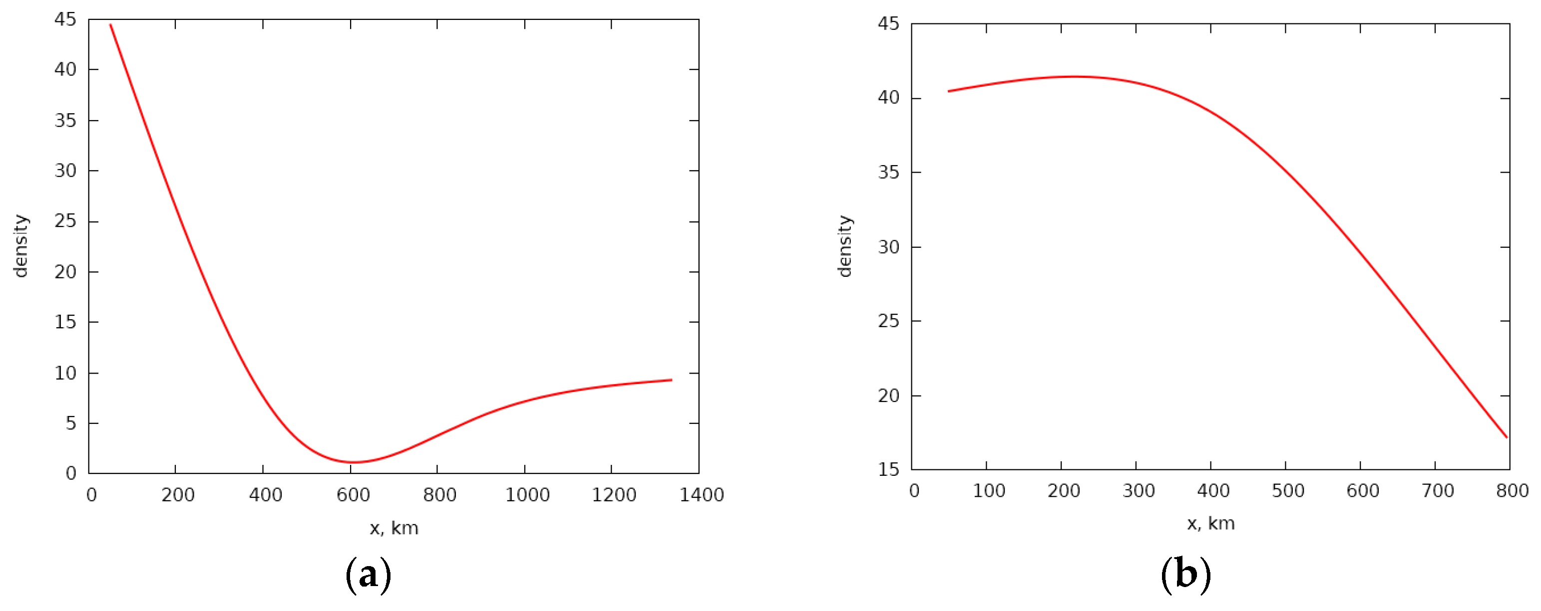
Linear density of population in Chile. (a)—to the north of Santiago. (b)—to the south of Santiago. The graphs were plotted through 4 points for North and 3 points for South excluding a data point for Santiago Metropolitan Region for clarity (population density in Santiago is approximately equal to 457 people per linear kilometer).
Figure 5.
Linear density of population in Chile. (a)—to the north of Santiago. (b)—to the south of Santiago. The graphs were plotted through 4 points for North and 3 points for South excluding a data point for Santiago Metropolitan Region for clarity (population density in Santiago is approximately equal to 457 people per linear kilometer).

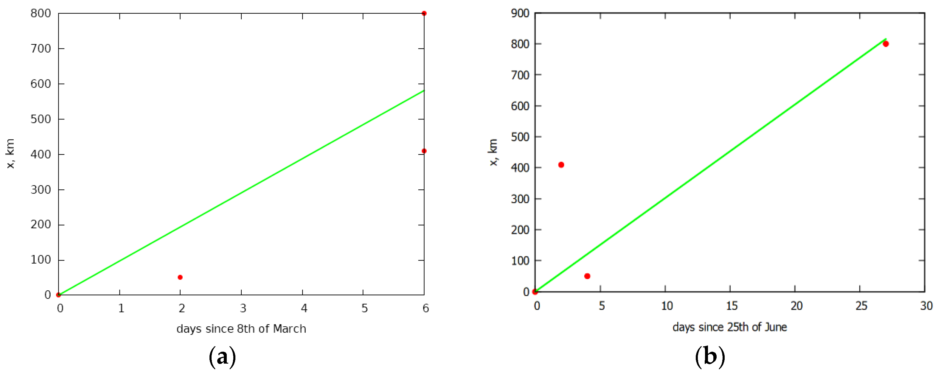
Figure 6.
Graphs for determining (a) speed of spread of the epidemic and (b) speed of recovery in southern Chile.
Figure 6.
Graphs for determining (a) speed of spread of the epidemic and (b) speed of recovery in southern Chile.

Figure 7.
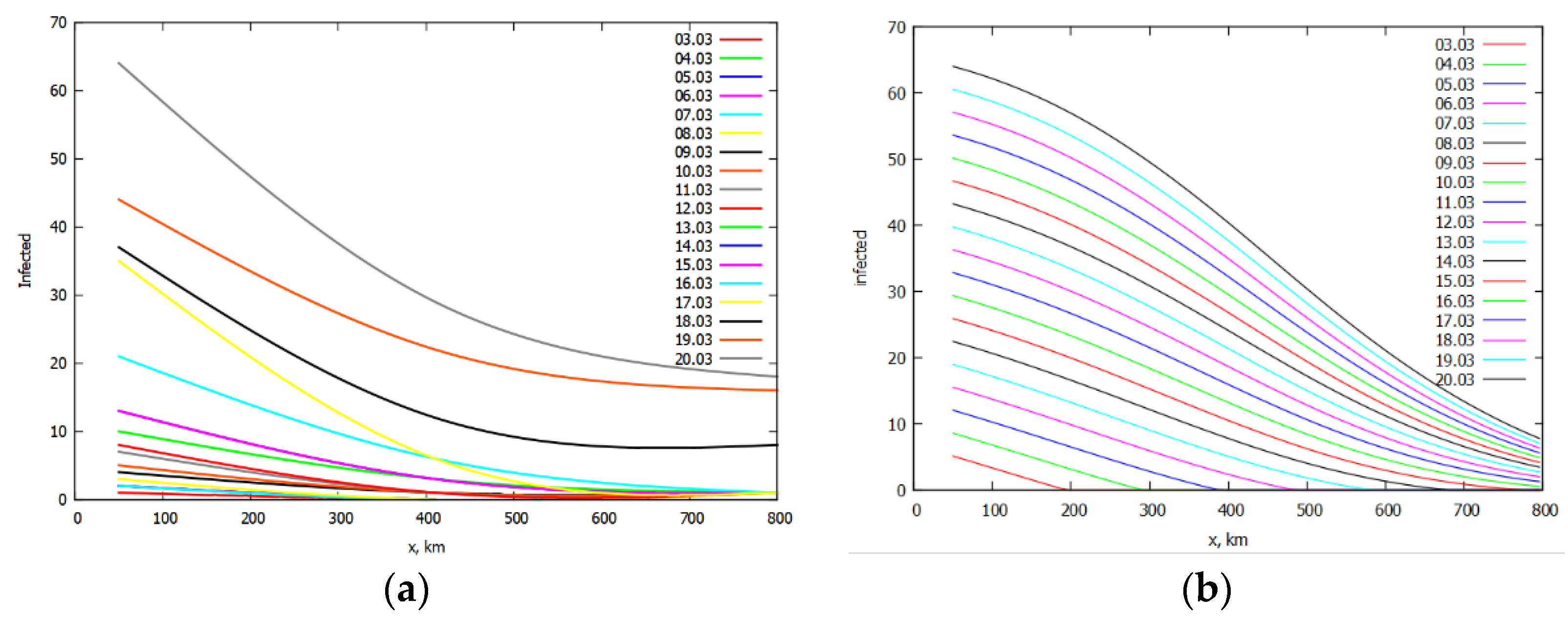
Graphs of for southern Chile. (a) Real data. (b) Theoretical results.

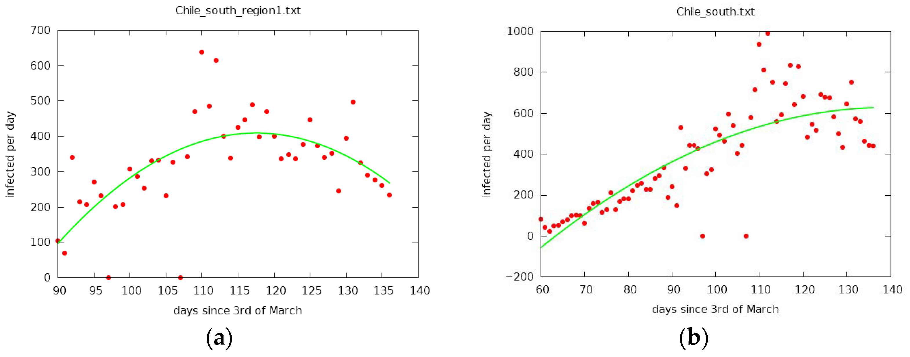
Figure 8.
Maximums of infection for (a) the first band and (b) south of Chile that correspond to maximums of parabolas. For the first band (a) the maximum is near the point 117 which means 28 June and for the South of Chile (b) it is near the point 140 which means 21 July.
Figure 8.
Maximums of infection for (a) the first band and (b) south of Chile that correspond to maximums of parabolas. For the first band (a) the maximum is near the point 117 which means 28 June and for the South of Chile (b) it is near the point 140 which means 21 July.

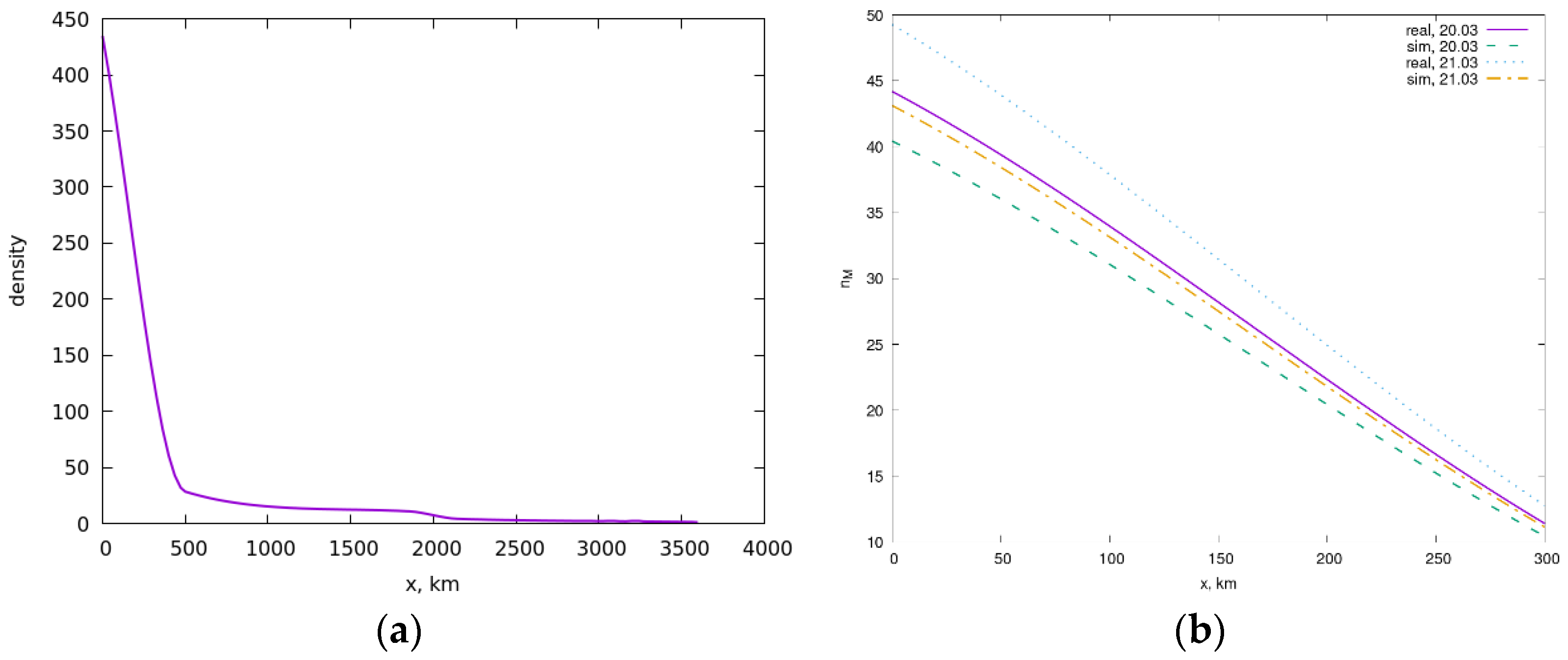
Figure 9.
(a) Linear density of population in Russia. (b) A closer look at real and theoretical data for the value for two subsequent days in Russia.
Figure 9.
(a) Linear density of population in Russia. (b) A closer look at real and theoretical data for the value for two subsequent days in Russia.

Figure 10.
Graphs for determining (a) speed of spread of the epidemic and (b) speed of recovery in Russia.
Figure 10.
Graphs for determining (a) speed of spread of the epidemic and (b) speed of recovery in Russia.

Figure 11.
Maximums of infection for (a) the first band and (b) all of Russia that correspond to maximums of parabolas. For the first band (a) the maximum is near the point 13 which means May 14 and for all of Russia (b) it is near the point 28 which means May 29.
Figure 11.
Maximums of infection for (a) the first band and (b) all of Russia that correspond to maximums of parabolas. For the first band (a) the maximum is near the point 13 which means May 14 and for all of Russia (b) it is near the point 28 which means May 29.

Figure 12.
Infections per day during second wave in (a) Moscow (maximum of parabola points to 10th of December) and (b) Russia, for which the maximum has not been reached yet and is expected to be reached sometime around 31st of December.
Figure 12.
Infections per day during second wave in (a) Moscow (maximum of parabola points to 10th of December) and (b) Russia, for which the maximum has not been reached yet and is expected to be reached sometime around 31st of December.

Figure 13.
Infections per day during second wave in (a) Moscow and (b) Russia with additional January data. The maximums are around 28 November for Moscow and 14 December for Russia.
Figure 13.
Infections per day during second wave in (a) Moscow and (b) Russia with additional January data. The maximums are around 28 November for Moscow and 14 December for Russia.


Table 1.
Regions to bands correspondence in Italy.
| № | Distance, km | Regions |
|---|---|---|
| 1 | 0 | Lombardy |
| 2 | 166 | Piedmont, Veneto, Emilia-Romagna, Liguria, Aosta Valley, Trentino-South Tyrol |
| 3 | 272 | Friuli Venezia Giulia, Tuscany |
| 4 | 376 | Marche, Umbria |
| 5 | 482 | Abruzzo, Lazio |
| 6 | 592 | Molise |
| 7 | 690 | Campania |
| 8 | 781 | Apulia, Basilicata |
| 9 | 933 | Calabria |
Table 2.
Regions to bands correspondence to the north of Santiago in Chile.
| № | Distance, km | Regions |
|---|---|---|
| 0 | 0 | Santiago |
| 1 | 50 | Coquimbo, Valparaíso |
| 2 | 470 | Atacama |
| 3 | 850 | Antofagasta |
| 4 | 1340 | Tarapacá, Arica and Parinacota |
Table 3.
Regions to bands correspondence to the south of Santiago in Chile.
| № | Distance, km | Regions |
|---|---|---|
| 0 | 0 | Santiago |
| 1 | 50 | O’Higgins, Maule, Ñuble |
| 2 | 470 | Biobío, Araucanía, Los Ríos |
| 3 | 850 | Los Lagos |
Table 4.
Regions to bands correspondence in Russia.
| № | Distance, km | Regions |
|---|---|---|
| 0 | Moscow, Moscow region | |
| 2 | 500 | Nizhny Novgorod Region, Ivanovo Region, Republic of Mordovia, Penza Region, Tambov Region, Volgograd Region, Ulyanovsk Region, Kostroma Region, Republic of Chuvashia, Republic of Mari El, Saratov Region |
| 3 | 1160 | Perm Territory, Republic of Komi, Republic of Bashkortostan, Orenburg Region, Samara Region, Republic of Tatarstan, Kirov Region, Nenets Autonomous District |
| 4 | 1850 | Tyumen region, Khanty-Mansi Autonomous Okrug, Kurgan region, Sverdlovsk region, Chelyabinsk region |
| 5 | 2150 | Omsk Region, Tomsk Region, Yamalo-Nenets Autonomous District, Novosibirsk Region |
| 6 | 3600 | Krasnoyarsk Territory, Irkutsk Region |
| 7 | 6000 | Khabarovsk Territory, Jewish Autonomous Region, Amur Re-gion, Primorsky Territory |
Publisher’s Note: MDPI stays neutral with regard to jurisdictional claims in published maps and institutional affiliations. |
© 2021 by the authors. Licensee MDPI, Basel, Switzerland. This article is an open access article distributed under the terms and conditions of the Creative Commons Attribution (CC BY) license (http://creativecommons.org/licenses/by/4.0/).
Share and Cite
MDPI and ACS Style
Aristov, V.V.; Stroganov, A.V.; Yastrebov, A.D. Simulation of Spatial Spread of the COVID-19 Pandemic on the Basis of the Kinetic-Advection Model. Physics 2021, 3, 85-102. https://0-doi-org.brum.beds.ac.uk/10.3390/physics3010008
AMA Style
Aristov VV, Stroganov AV, Yastrebov AD. Simulation of Spatial Spread of the COVID-19 Pandemic on the Basis of the Kinetic-Advection Model. Physics. 2021; 3(1):85-102. https://0-doi-org.brum.beds.ac.uk/10.3390/physics3010008
Chicago/Turabian StyleAristov, Vladimir V., Andrey V. Stroganov, and Andrey D. Yastrebov. 2021. "Simulation of Spatial Spread of the COVID-19 Pandemic on the Basis of the Kinetic-Advection Model" Physics 3, no. 1: 85-102. https://0-doi-org.brum.beds.ac.uk/10.3390/physics3010008