Comparison of Main Covid-19 Outbreaks and Interpretation Based on Age Differences


ENEA—Fusion and Nuclear Safety Department, Via E. Fermi 45, 00044 Frascati, Italy
*
Author to whom correspondence should be addressed.
Physics 2021, 3(1), 119-127; https://0-doi-org.brum.beds.ac.uk/10.3390/physics3010010
Submission received: 19 January 2021
/
Revised: 5 March 2021
/
Accepted: 10 March 2021
/
Published: 16 March 2021
(This article belongs to the Special Issue Physics Methods in Coronavirus Pandemic Analysis)
Abstract
:The main scope of this study is a critical comparison of data coming from different regions in the world, where significant outbreaks of the Covid-19 pandemic took place, accounting for age differences among the considered samples. Scaling laws are derived, driving interpretations of the death toll in the analyzed clusters.
1. Introduction
The Covid-19 epidemic stands as a unique case in human history: it is the first time that a very infectious pathology has spread within a highly globalized environment. After the first outbreak in the Hubei region of China, the virus hit the Italian region of Lombardy in March. Since no past record can be retrieved, one way to understand the Italian spread rate is to use the only previously available data: those from China, where the epidemic took place more than one month earlier.
From official data, the death toll was surprisingly high in Lombardy, if compared with Hubei data. Despite a couple of differences, at first approximation the two outbreaks are comparable, and a similar number of cumulative deaths was expected. In particular, this should have happened in the first period, before any impact of lockdown measures or differences in the health system starts to bias the data time evolution.
The goal of this study is to prove that the difference on the cumulative death toll between Lombardy and Hubei can be explained mostly considering the age difference of the two populations.
2. Data Samples and Methodology
2.1. Samples and Variables
The comparison was made between the single outbreaks experienced in January and March, respectively in Hubei and Lombardy. Table 1 shows features of the two regions. Despite differences in population and area extents, the population density is comparable.
The comparison could be done on three quantities:
- number of infected people;
- number of people in intensive care;
- number of dead people.
The number of infected people is not a good universal estimator, as it depends on the number of tested ones, and subsequently on the ways people are tested and declared positive: for instance, after 12 February, in Hubei the number of positive people was determined only using symptomatology and chest X-rays, without the nose pharyngeal swab tests.
The number of people under intensive therapy depends on the bed capacity, which in turn is difficult to compare between countries with different Healthcare systems and services. In light of these considerations, the number of dead people results in the crudest but also the most significant estimator adopted in the present work for a quantitative comparison.
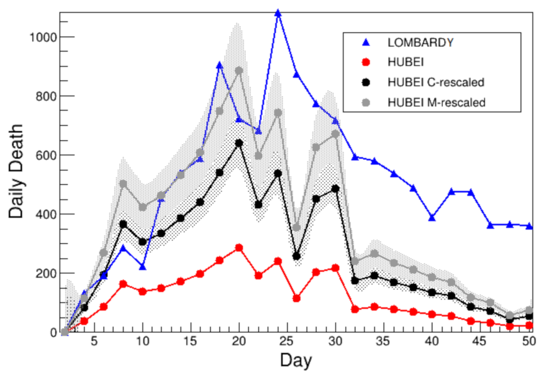
Figure 1 shows the comparison of the cumulative number of deaths between Lombardy [4] (blue) and Hubei [5] (red), while Figure 2 shows the comparison of the two-day victims number, in the two regions. The first day considered is conventionally that when 100 cumulative deaths has been exceeded: 28 January in Hubei and 6 March in Lombardy, 37 days later. By looking at both Figure 1 and Figure 2 it is clear how the number of deaths in Lombardy exceeded those in Hubei data.
Different hypotheses have been considered to understand this behavior:
- lockdown decision delayed for too long a time in Italy;
- Italian Healthcare system not equipped enough or unfit to face an epidemic;
- differences in the mean population age, between China and Italy.
2.2. Age Ranges
The goal of the present work is to understand whether—at first approximation—the difference between Hubei and Lombardy in the cumulative death toll can be explained by age difference.
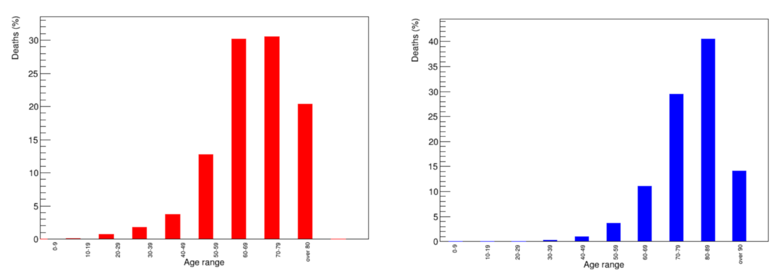
The mean population age in China is 37 years old as reported in 2019 [6], while in Italy is 45 years old as reported in 2018 [7]. Consequently, during the first months of the pandemic, the mean victim age (MVA) in Italy is around 80 years old [8], while for China, from data sorted according to population age [9], the MVA is estimated to be 70 years. Similar age differences were found checking the infected people mean age, about 50 in China [10] and 62 for Italy [8]. Table 2 shows the comparison of mean ages in the early months of the pandemic, between the two countries. Figure 3 shows the distribution of the number of victims per age category [8,9]. The mean victims age is the quantity to be elaborated further on, in the following.
2.3. Methodology
The idea of this work is to use the Hubei data as the starting point to build a model to be compared with other outbreaks, in particular with the Italian one, under the hypothesis that at first approximation the number of victims for different outbreaks depends mainly on the age distribution of deaths. Linear extrapolation is used to morph the Hubei data distribution to a different age range. This is a common methodology in Physics [11,12], also widely used in most of the other research fields. Extrapolation is performed daily multiplying the actual number of victims by a proper scale factor,
to obtain a time evolution of the cumulative number of victims, corrected accounting for a population age different from the starting sample. Here, the actual number of deaths in Hubei is rescaled as if this region population had a different mean age. The scale factor is the parameter that needs to be estimated. in the present work, it is defined as
where is the mortality—namely the ratio between the number of deaths and the number of infected cases—for the specified k age range, and is the real age of the starting sample.
Available data [10] on the population mortality M are stratified in ranges of ten years based on the age, and could be obtained in different ways: for the moment the crude estimate method is used, so mortality is simply the ratio between deaths and infected people numbers. Impact from this choice rather than others is discussed in Section 4.
Since in China the MVA is about 70 years (as discussed in Section 2.2), three hypotheses are made:
- 60–70 range, discussed in Section 3.1, with ;
- 70–80 range, discussed in Section 3.2, with ;
- average, an average of the previous ones, discussed in Section 3.2, with .
In Section 3.1 the assignment is done. The other two hypotheses are discussed in Section 3.2. Since Italy has the MVA equal to 80 years, three assignment hypotheses are considered:
- the optimistic 70–80 range where ;
- the pessimistic 80–90 range where ;
- the average of the previous ones where .
It is possible to define a total of nine rescale factors, using the three hypotheses for China age range assignment times three hypotheses for Italy age range assignment.
3. Analysis
Data from the Hubei region provide the model to be compared to those from the Lombardy region. In principle, this comparison can be performed based on nine possible age assignment combinations, as there are three range hypotheses for both China and Italy.
3.1. China in 60–70 Range
The first hypothesis is the 60–70 range assignment to China: . The three assignments to the Italian age are discussed as follows.
3.1.1. Italian Optimistic Assignment (C-Rescale)
The first hypothesis for Italy is to assign the 70–80 years range mortality to Italy. Then, the actual number of deaths in Hubei is rescaled as if this region population were 10 years older, adopting the range instead of the , previously considered as the MVA is 66 years in China. This estimate is computed using the mortality ratio between the two intervals in Hubei, as the scale factor:
The scale factor is defined as a conservative rescale (C-rescale)
where death toll in China are and . The uncertainties on the mortality factor are evaluated using the Gaussian approximation from [10], and the uncertainty on the scale factor is determined through error propagation. Figure 1 shows the comparison of the cumulative number of deaths among Lombardy (blue), actual Hubei (red) and Hubei rescaled (black) according to Equation (2), while Figure 2 shows the comparison of the two-day number of deaths among the same regions.
3.1.2. Italian Average Assignment (M-Rescale)
Since in Italy the MVA is about 80 years, assigning the 70–80 years range mortality in the numerator of Equation (2) is a slightly optimistic choice, as mentioned before.
A different hypothesis [10] is to use the average mortality between 70–80 and 80–100 ranges, i.e., , so that the scale factor results in
where again uncertainties are obtained in Gaussian approximation. This choice of an average mortality is defined M-rescale. Figure 1 shows the comparison between this estimate (gray) and those previously discussed in terms of the cumulative number of deaths.
Figure 2 shows the comparison of the two-day number of deaths, among the same categories in the latter Figure.
3.1.3. Italian Pessimistic Assignment (NC-Rescale)
The third hypothesis is formulated by assigning the 80–100 years range mortality to the Lombardy region, , so that the related scale factor is:
and it is defined as a pessimistic non-conservative NC-rescale factor. Figure 1 shows the comparison between this estimate (brown) and the previously discussed ones for the cumulative number of deaths.The curves of growth of Lombardy and NC-rescaled Hubei have a very similar behavior. For more consistent a comparison, Figure 1 suggests that a proper treatment of the counts as a function of time must be applied. This is explained in the following Section 3.1.4.
3.1.4. Time Offset
Since the starting day for each population is a conventional choice, it is possible to shift in time one distribution with respect to the others: in this way, the first day is synchronized among different samples. The adopted time offset is the first day in which both Lombardy and NC-rescaled Hubei exceed the number of 1500 deaths, instead of the 100 deaths previously used. This approach is equivalent to move the Lombardy distribution 5 days back in time, namely starting from 11 March. As a result of this choice, the agreement between Lombardy and NC-rescaled Hubei is very good, especially in the rising part of the curve, as shown in Figure 4.
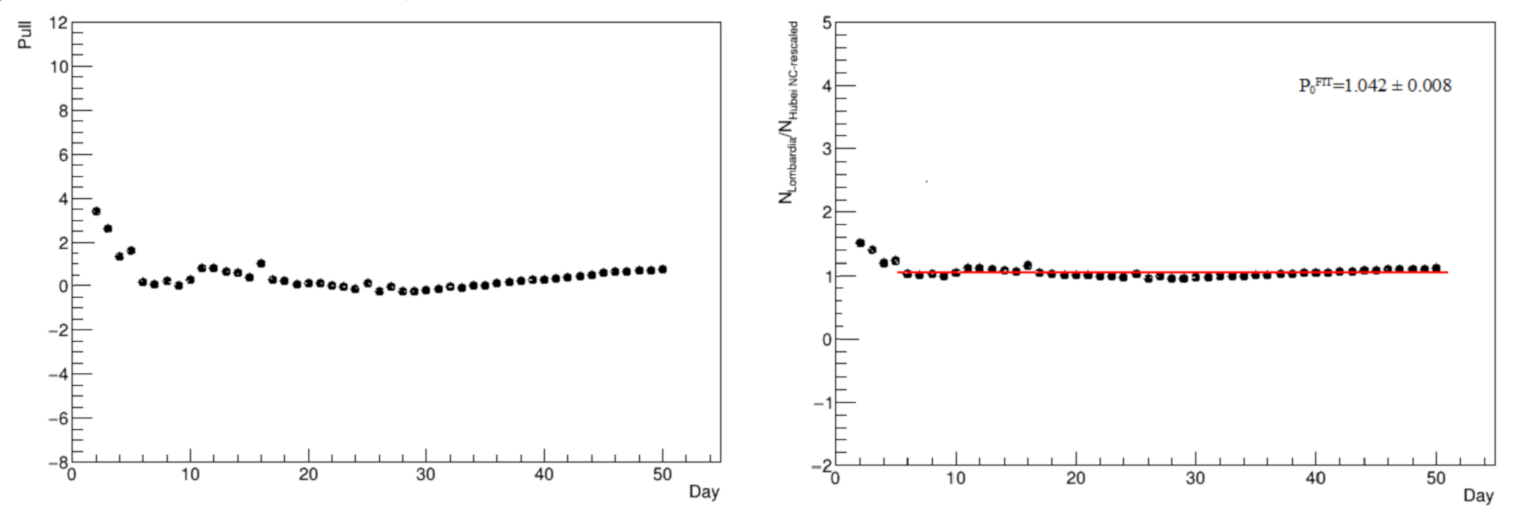
The comparison between Lombardy and NC-rescaled Hubei is studied in detail by evaluating the pull in Figure 5 (left panel), namely the difference divided by the uncertainty, dominated by the systematic one associated with the scale factor, and the ratio of the two distribution entries in Figure 5 (right panel). In this latter case, a constant term is fit to the ratio, to estimate the fractional difference between the two distributions, at least starting from a time period where the agreement tends to be good: from a common time defined as the 5th day, the two distributions have an average overall difference of .
3.2. Other Age Assignments for China
As already discussed in Section 2.3, other two hypotheses for the China age range can be done: the 70–80 range () and the average one, where . Since, three age ranges are also possible for Italy, the number of scale factor combinations is six, in addition to the three already discussed in Section 3.1:
As can be seen, is consistent with , within uncertainty. Thus, the result is almost the same discussed in Section 3.1.1. All other values are lower than the result discussed in Section 3.1, as expected. Since good agreement with the Lombardy data is found only with the highest scale factor, any other value will result in a disfavored fit and so it is not investigated further.
4. Systematic Uncertainties Evaluation and Control Sample
The main systematic uncertainty of this study is due to the scale factor calculation that depends on the mortality estimate method.
It is possible to vary the criterion of the mortality calculation to check the dependence of the scaling factor. In reference [10] four different criteria are presented:
- crude estimation (CrE), used in the analysis;
- adjusted for delayed mortality (ADJ1);
- adjusted for unidentified symptomatic cases (ADJ2);
- adjusted for both (ADJ3).
Details in the description of these criteria are beyond the scope of the present analysis. The main message conveyed here is that a different scale factor is associated with each of the four criteria.
Starting with the conservative scaling, the results of are the following:
in very good agreement within one another within the uncertainties.
For the non-conservative scaling, the results for are the following:
also, in this case—namely the scale factor that yields the best agreement between Lombardy and rescaled Hubei—whatever choice is in very good agreement with the others within the uncertainties.
Since it is just the average of the previous results, by construction the M-rescale factor turns to be consistent against any choice of the four criteria, and no explicit check is reported. As a result of these checks, no dependence on the mortality estimate method is found on the way scaling factors are evaluated.
To validate the concept behind the presented scale technique—based on demographic considerations—it is important to identify an independent control sample, with features similar but not completely equivalent to Hubei and Lombardy: population density, healthcare system, single outbreak, mean population age, sufficient statistics. The selected control sample is the state of New Jersey in the USA, as it bears features similar to Lombardy.
Table 3 shows the main features of interest for the present analysis. Since the New Jersey MVA is slightly lower but close to 80 years, an agreement with either the C-rescaled or the M-rescaled Hubei is likely to be expected.
Figure 4 shows all results discussed so far on the cumulative number of victims plus the curve related to New Jersey. In the latter, the starting day is 27 March, when more than 100 deaths have been recorded.
Good agreement with the C-rescaled Hubei behavior is found during the first four weeks, expected as mentioned before. After this first month, the curve suddenly changes slope, starting to grow as fast as the M-rescaled Hubei behavior. As already said, this can be understood considering that New Jersey MVA is close to the upper limit of the 70–80 years range, such that a good description lies in between the C-rescaled and M-rescaled Hubei distributions. The steep rise of victims after about one month in New Jersey is also probably due to the differences in the lockdown procedure implemented in the USA with respect to the rigid one applied in China. When compared to Lombardy, possible sources of difference must be investigated within a younger mean population age, closely related to a younger mean infected age.
5. Results
This study demonstrates that to a very good approximation the difference in the cumulative number of deaths between Lombardy and Hubei can be explained by taking only the age difference of the two populations into account, and rescaling by means of the mortalities ratio between the two samples. Independence from the mortality calculation method is also proven. Nine scaling possibilities are tested, depending on the age range choice for both Chinese and Italian mortality. After having corrected the Lombardy starting day to achieve consistent time synchronization with Hubei, a quite good agreement is obtained between the victim growth curves of the two populations. This happens with the largest rescale factor out of the tested hypotheses for China. Thus, the mean age difference does not explain exhaustively the analyzed behaviors.
One control sample is used to test the main concept behind this procedure: New Jersey in the USA, which has similar area and population density values compared to Lombardy. Good agreement with the Hubei rescaled conservatively is found, as expected since both regions have lower age features than Italy in both mean population and victims age in New Jersey. Another relevant aspect is that lockdown measures in the USA were generally softer than in China. Of course, every single outbreak brings aspects that cannot be exhaustively explained only by means of mere demographic considerations.
The same methodology can be applied to other studies that compare data from the Covid-19 pandemic, after having quantitatively investigated and identified possible sources of difference between two outbreaks sharing similar properties, such as the population density.
In the present work, the age interval is assigned to each population. Then, the mortality ratio of the two samples for the different age range is used to estimate scale factors that can be applied to one or both samples, for an improved comparison.
In conclusion, a simple method of rescaling according to mortality factors can explain large portions of the death toll rise in different countries, with similar demographic characteristics in terms of area and population density.
Author Contributions
Conceptualization, F.N. and A.S.; methodology, F.N. and A.S.; software, F.N. and A.S.; validation, F.N. and A.S.; formal analysis, F.N. and A.S.; investigation, F.N. and A.S.; resources, F.N. and A.S.; data curation, F.N. and A.S.; writing—original draft preparation, F.N. and A.S.; writing—review and editing, F.N. and A.S.; visualization, F.N. and A.S.; supervision, F.N. and A.S.; project administration, F.N. and A.S.; funding acquisition, F.N. and A.S. All authors have read and agreed to the published version of the manuscript.
Funding
This research received no external funding.
Data Availability Statement
Data are contained within the article and collected from the references listed in the bibliography.
Acknowledgments
The authors would like to thank their colleague Francesco Napoli for many useful discussions.
Conflicts of Interest
The authors declare no conflict of interest.
References
- Monthly Demographic Balance, January–June 2013. Available online: http://demo.istat.it/bil/index.php?anno=2013&lingua=eng (accessed on 2 April 2020).
- “Hubei Survey”, Ministry Of Commerce—People’s Republic of China. Available online: https://web.archive.org/web/20180406185510/http://english.mofcom.gov.cn/aarticle/zt_business/lanmub/200704/20070404609936.html (accessed on 2 April 2020).
- Communiqué of the National Bureau of Statistics of People’s Republic of China on Major Figures of the 2010 Population Census. National Bureau of Statistics of China. Available online: https://web.archive.org/web/20130727021210/http://www.stats.gov.cn/english/newsandcomingevents/t20110429_402722516.htm (accessed on 2 April 2020).
- Coronavirus Emergency Situation Map. Available online: https://github.com/pcm-dpc/COVID-19 (accessed on 2 April 2020).
- COVID-19 Dashboard by the Center for Systems Science and Engineering at Johns Hopkins University. Available online: https://github.com/CSSEGISandData/COVID-19 (accessed on 2 April 2020).
- Data from United Nations—Department of Economic and Social Affairs—Population Dynamics. Available online: https://population.un.org/wpp/DataQuery/ (accessed on 2 April 2020).
- Data from Eurostat. Available online: https://ec.europa.eu/eurostat/data/database (accessed on 2 April 2020). (In Italian).
- Available online: https://www.epicentro.iss.it/coronavirus/bollettino/Infografica_24aprile%20ITA.pdf (accessed on 2 April 2020). (In Italian).
- Zhang, Y. Vital Surveillances: The Epidemiological Characteristics of an Outbreak of 2019 Novel Coronavirus Diseases (COVID-19)—China, 2020. China CDC Wkly. 2020, 2, 113–122. Available online: http://weekly.chinacdc.cn/en/article/id/e53946e2-c6c4-41e9-9a9b-fea8db1a8f51 (accessed on 2 April 2020).
- Riou, J.; Hauser, A.; Counotte, M.J.; Althaus, C.L. Adjusted Age-Specific Case Fatality Ratio during the Covid-19 Epidemic in Hubei, China, January and February 2020. Available online: https://www.medrxiv.org/content/10.1101/2020.03.04.20031104v1.full.pdf (accessed on 2 April 2020).
- James, F.E. Statistical Methods in Experimental Physics; World Scientific: Singapore, 2006. [Google Scholar]
- Frodesen, A.G.; Skjeggestad, O.; Tøfte, H. Probability and Statistics in Particle Physics; Universitetsforlaget: Bergen, Norway, 1979. [Google Scholar]
- Available online: https://www.nj.gov/health/cd/documents/topics/NCOV/COVID_Confirmed_Case_Summary.pdf (accessed on 2 April 2020).
Figure 1.
Comparison of the cumulative number of deaths among Lombardy (blue), Hubei (red), C-rescaled Hubei (black), M-rescaled Hubei (gray) and NC-rescaled Hubei (brown). Error bands are due to the proper scale factor uncertainty. The abscissa axis is the number of days after the first day considered (see Section 2.1 for details).

Figure 2.
Comparison of the two-day number of deaths Lombardy (blue), Hubei (red), C-rescaled Hubei (black) and M-rescaled Hubei (gray). Error bands are due to the proper scale factor uncertainty. The abscissa axis is the number of days after the first day considered (see Section 2.1 for details).
Figure 2.
Comparison of the two-day number of deaths Lombardy (blue), Hubei (red), C-rescaled Hubei (black) and M-rescaled Hubei (gray). Error bands are due to the proper scale factor uncertainty. The abscissa axis is the number of days after the first day considered (see Section 2.1 for details).

Figure 3.
Age distribution of Covid victims (in percentage) in China (red) and Italy (blue). In case of China, only one range over 80 years old is available [9], while for Italy both 80–90 and over 90 ranges are reported [8].

Figure 4.
Comparison of the cumulative number of deaths among Lombardy moved 5 days back in time (blue), Hubei (red), C-rescaled Hubei (black), M-rescaled Hubei (gray), NC-rescaled Hubei (brown) and New Jersey (dark blue). Error bands are due to the proper scale factor uncertainty. The abscissa axis is the number of days after the first day considered (see Section 2.1 and Section 3.1.4 for details).

Figure 5.
Left: Time profile of the pull distribution between Lombardy and NC-rescaled Hubei. Right: Time profile of the ratio, fit to a constant term.
Figure 5.
Left: Time profile of the pull distribution between Lombardy and NC-rescaled Hubei. Right: Time profile of the ratio, fit to a constant term.


Table 1.
Region features.
| Lombardy [1] | Hubei [2,3] | |
|---|---|---|
| Area (km) | 23,844 | 185,900 |
| Population | 10,103,969 | 58,500,000 |
| Density (km) | 420 | 310 |
Table 2.
Mean age comparison.
| Italy | China | |
|---|---|---|
| Population age | 45 | 37 |
| Infected people age | 62 | 55 |
| Victims age | 80 | 70 |
Table 3.
New Jersey features [13].
Table 3.
New Jersey features [13].
| Area (km) | 22,608 |
| Population | 8,908,520 |
| Density (km) | 394 |
| Mean population age | 40 |
| Mean infected age | 68 |
| Mean victims age | 78 |
Publisher’s Note: MDPI stays neutral with regard to jurisdictional claims in published maps and institutional affiliations. |
© 2021 by the authors. Licensee MDPI, Basel, Switzerland. This article is an open access article distributed under the terms and conditions of the Creative Commons Attribution (CC BY) license (http://creativecommons.org/licenses/by/4.0/).
Share and Cite
MDPI and ACS Style
Nguyen, F.; Selce, A. Comparison of Main Covid-19 Outbreaks and Interpretation Based on Age Differences. Physics 2021, 3, 119-127. https://0-doi-org.brum.beds.ac.uk/10.3390/physics3010010
AMA Style
Nguyen F, Selce A. Comparison of Main Covid-19 Outbreaks and Interpretation Based on Age Differences. Physics. 2021; 3(1):119-127. https://0-doi-org.brum.beds.ac.uk/10.3390/physics3010010
Chicago/Turabian StyleNguyen, Federico, and Andrea Selce. 2021. "Comparison of Main Covid-19 Outbreaks and Interpretation Based on Age Differences" Physics 3, no. 1: 119-127. https://0-doi-org.brum.beds.ac.uk/10.3390/physics3010010