Adaptive Synchronization of Fractional-Order Complex-Valued Chaotic Neural Networks with Time-Delay and Unknown Parameters

1
College of Physics, Hebei Normal University, Shijiazhuang 050024, China
2
Department of Computer Science, North China Electric Power University, Baoding 071003, China
3
College of Physics and Electronic Engineering, Xingtai University, Xingtai 054001, China
*
Author to whom correspondence should be addressed.
Physics 2021, 3(4), 924-939; https://0-doi-org.brum.beds.ac.uk/10.3390/physics3040058
Submission received: 2 August 2021
/
Revised: 27 September 2021
/
Accepted: 30 September 2021
/
Published: 12 October 2021
(This article belongs to the Section Applied Physics)
Abstract
:The purpose of this paper is to study and analyze the concept of fractional-order complex-valued chaotic networks with external bounded disturbances and uncertainties. The synchronization problem and parameter identification of fractional-order complex-valued chaotic neural networks (FOCVCNNs) with time-delay and unknown parameters are investigated. Synchronization between a driving FOCVCNN and a response FOCVCNN, as well as the identification of unknown parameters are implemented. Based on fractional complex-valued inequalities and stability theory of fractional-order chaotic complex-valued systems, the paper designs suitable adaptive controllers and complex update laws. Moreover, it scientifically estimates the uncertainties and external disturbances to establish the stability of controlled systems. The computer simulation results verify the correctness of the proposed method. Not only a new method for analyzing FOCVCNNs with time-delay and unknown complex parameters is provided, but also a sensitive decrease of the computational and analytical complexity.
1. Introduction
Compared with real-valued neural networks, complex-valued neural networks have the advantages of simpler network structure, simpler training process, and stronger ability to handle complex signals. This is mainly due to the fact that the state vectors, connection weights, and activation functions in complex-valued neural networks are all represented by complex values. In addition, complex-valued neural networks can solve problems that cannot be solved by real-valued neural networks. For example, two-layer real-valued neural networks cannot solve the problems of exclusive “OR” (XOR) and symmetry detection, while two-layer complex-valued neural networks can easily do so, which shows that the computational ability of complex-valued neurons is remarkable. In recent years, practical applications of complex-valued neural networks in physical systems such as electromagnetic, optical, ultrasonic, and quantum waves, as well as in the fields of filtering, speech synthesis, and remote sensing, have attracted widespread attention [1,2,3,4,5,6,7,8,9,10,11,12,13,14,15,16,17,18,19].
With the development of fractional calculus, more and more researchers recognize that fractional-order models can better describe various substances and processes with memory and genetic properties in neural networks than integer-order models, and can also effectively facilitate the information process. Meanwhile, fractional-order calculus in neural networks can improve the accuracy and flexibility of computation, and have a great application value in computational optimization and control performance improvement. Therefore, combining fractional-order calculus with neural network models to form fractional-order neural network models expands the basic theory and application capabilities of neural networks.
The analysis of fractional-order neural networks (FNNs) has become a research area attracting increasing interest (see [20,21,22,23,24,25,26,27,28,29,30,31,32,33,34,35,36,37,38,39,40] and references therein). Moreover, the simultaneous analysis of stability of fractional-order real-valued and complex-valued neural networks has received extensive attention. In [20,21], projection synchronization and adaptive synchronization of fractional-order memristor neural networks are discussed. In [10], synchronization of fractional-order complex-valued neural networks (FOCVNNs) was studied using the linear delay feedback control. The authors investigated the global Mittag-Leffler synchronization problem of fractional-order neural networks in Refs. [22,23,24]. In Refs. [25,26,27,28,29,30,31,32], the authors analyzed the stability, finite-time stability, and global Mittag-Leffler stability of fractional-order time-delayed complex-valued neural networks, respectively. In [31], several sufficient conditions for achieving finite-time projection synchronization of fractional-order complex-valued neural networks are derived by applying set-valued mappings, differential inclusion theory, and Gronwalls’ inequality. In [32], Li et al. implemented the adaptive synchronization of fractional-order complex-valued neural networks with discrete and distributed delays. The modified function projective synchronization (MFPS) for complex dynamical networks with mixed time-varying and hybrid asymmetric coupling delays was investigated in [33]. In [34], the authors studied a novel delay-dependent asymptotic stability of a differential and Riemann-Liouville fractional differential neutral system with constant delays and nonlinear perturbation. In [35], Dai et al. reported that in populations with cooperative and competitive oscillators, the transition between continuous and explosive can be tuned simply by adjusting the balance between the two oscillator types. Furthermore, Dai et al. [36] proposed a unified framework for the analysis of system synchronization and conducted an in-depth study of network synchronization laws in different dimensions.
It should be noted that the aforementioned papers on neural network synchronization all assume that the network is predetermined. In fact, in many practical engineering situations, most system parameters cannot be accurately determined in advance, and chaotic synchronization will be disrupted by these uncertainties. In addition, there are usually delays in neural networks due to the limited speed of signal transmission between neurons. Time-delay can have an impact on the dynamic properties of a neural network and can even destroy it. Although, authors in [37] investigated the controller design problem for finite-time and fixed-time stabilization of fractional-order memristive complex-valued bidirectional associative memory (BAM) neural networks with uncertain parameters and time-varying delays, but the nonlinear complex-valued activation functions are split into two (real and imaginary) components. Therefore, to the best of our knowledge, there are few studies on the synchronization of fractional-order complex-valued chaotic neural networks (FOCVCNNs) with time-delays and unknown parameters, especially without dividing the real and imaginary components into two real-valued systems. Therefore, it is very important and useful to efficiently synchronize fractional-order complex-valued chaotic neural networks with time-delays and unknown parameters in practical applications.
Inspired by the above discussion, this paper investigates the synchronization problem of FOCVCNNs with time-delay and unknown complex parameters. Using inequalities containing fractional-order derivatives of complex variables and the stability theory of fractional-order complex-valued chaotic systems, synchronization and parameter identification of FOCVCNNs are achieved.
The main contributions of this paper can be summarized as follows.
- (i)
- Most of the existing studies on the synchronization methods of fractional-order neural networks are about fractional-order real-valued neural networks. On the other hand, existing studies on fractional-order complex-valued neural networks are on the known parameters or with no time-delay or without identifying the parameters.
- (ii)
- A new adaptive controller and update laws are designed to synchronize the driving and response systems. This is the first study of synchronization of fractional-order complex-valued neural networks with time-delay and unknown complex parameters.
- (iii)
- Compared with previous synchronization models of fractional-order complex neural networks, the model proposed in this paper is more tractable and easier to be implemented in practical systems.
- (iv)
- For fractional-order complex neural networks with known parameters and time-delay or known parameters without time-delay, the synchronization model proposed in this paper is also applicable, and only the control strategies need to be adjusted accordingly.
- (v)
- This paper proposes the novel perspective that chaos occurs in fractional-order complex-valued neural networks as long as the parameters are suitable, and two new FOCVCNNs are given to broaden the application of fractional-order complex-valued neural networks.
2. Preliminaries
Fractional calculus plays an important role in modern science. In this paper, Riemann-Liouville and Caputo’s fractional operators are used as the main tools.
Notation: denotes a complex n-dimensional space. For , and are the real part, imaginary part, and conjugate of , respectively.
Definition 1
([41]). The fractional integral form of order α for function is defined as follows:
where denotes the time and is the initial time, , and > 0.
Definition 2
([41]). Caputo’s fractional derivative form of order for function is defined by:
where t t0 and n are a positive integer, then .
Lemma 1.
Lemma 2.
(Stability theory for fractional-order system [41]). Letbe a uniformly continuous and derivable Lyapunov function, and letbe a derivable and nonnegative function.
If
and
whereis a positive constant. Then,.
Lemma 3
Remark 1.
Since, as, if, one can deduce Lemma 2, by this Lemma.
Lemma 4
3. Main Results
Let us consider a kind of FOCVCNNs described by the following equations:
where , and is the complex state variable of the ith neuron; represent the activation functions without and with delay; denote the connection weight and delayed connection weight, respectively; are constant delays; and represents the corresponding external inputs. The complex-valued functions and satisfy the following assumptions.
Assumption 1.
For any, there exist real numbers> 0, then
Assumption 2.
For any, there exist real numbers> 0 and>0, then
Choose system (9) as the master system, and are unknown constants which need to be identified, then the controlled response system is given by:
where is the complex state variable of the ith neuron of the response system; represent the estimated connection weights and delayed connection weights, respectively; and are controllers to be determined.
Let be the synchronization errors between master system (9) and slave system (12), then one can get the following error dynamical system:
Theorem 1.
If Assumptions 1 and 2 hold, the asymptotic synchronization and parameter identification of systems (9) and (12) can be achieved under adaptive controllers, described as Equation (14) and adaptive update laws (15)–(18):
whereare positive constants.
Proof.
Let us present the following Lyapunov functional candidate:
where are two positive constants to be determined. □
Using Lemma 1:
Along with Equation (13) and qualities (14)–(18), one gets:
According to Lemma 4 and Assumption 1:
Letting :
From Lemma 2 or Lemma 3, one can obtain: , indicating , which shows that systems (9) and (12) can obtain asymptotic synchronization. Meanwhile, according to Remark 1 of Theorem 1 of Ref. [45], the parameter identification is achieved.
Remark 2.
Theorem 1provides a stability criterion for fractional-order nonlinear uncertain systems with time-delay by choosing a Lyapunov function that includes V1(t) and V2(t).
Remark 3.
Theorem 1provides a Lyapunov-based adaptive control method for stability analysis and synchronization of FOCVCNNs.
Remark 4.
Lemma 3is applied to verify the stability of fractional-order with unknown parameters and external disturbances, as well as to the design of synchronous controllers for these systems.
Remark 5.
For FOCVCNNs with known parameters, the update laws will be reduced to (14) and (15).
Remark 6.
For FOCVCNNs with known parameters and without time-delay, the synchronization between systems (9) and (12) can be achieved under the following control strategy (24).
Remark 7.
It is worth mentioning that the synchronization problem discussed in this paper is about fractional-order complex-valued neural networks with time-varying delays and unknown parameters, while most of the existing work on parameter identification methods for synchronization is about fractional-order real-valued models. On the other hand, previous studies have mainly focused on fractional-order complex-valued models with known parameters [10,31,43] or fractional-order complex-valued models without time-delay [46]:
where is a positive constant.
4. Numerical Simulations
In this Section, several numerical examples of fractional-order complex-valued neural networks are given to show the effectiveness of the scheme proposed in previous Sections. For the numerical solution of these systems, the predictor–corrector method [45] of the MATLAB platform is adopted. The Lyapunov exponents of systems are calculated by the algorithm of Wolf et al. [47], with some adaptations.
Example 1.
Consider a class of FOCVCNNs, which is described as follows:
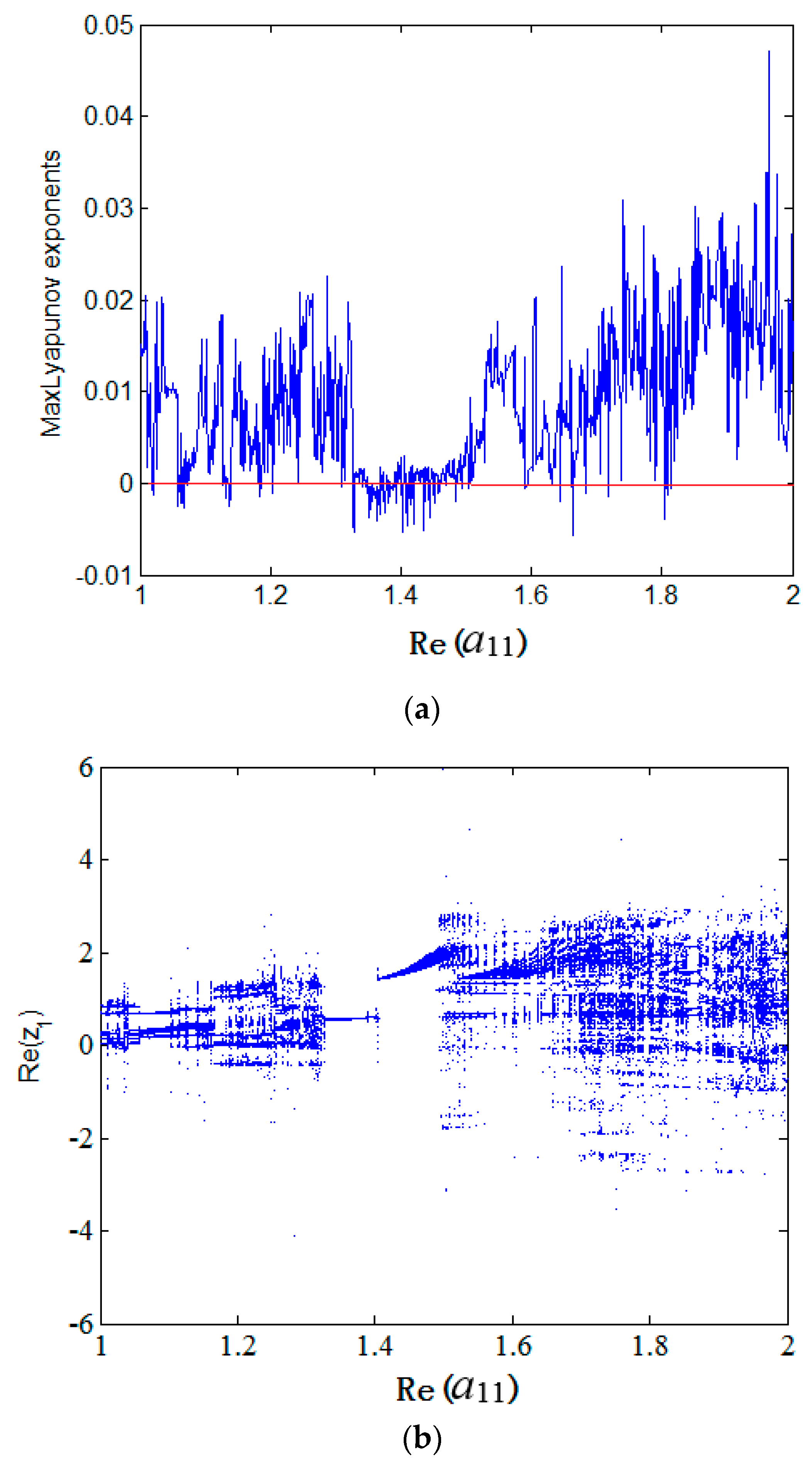
If one selects , , , , , , , then let . Figure 1a depicts the maximum Lyapunov exponent (MLE) spectrum of system (25), and Figure 1b shows its bifurcation diagram. Figure 1 shows that system (25) is chaotic at fractional-order, .
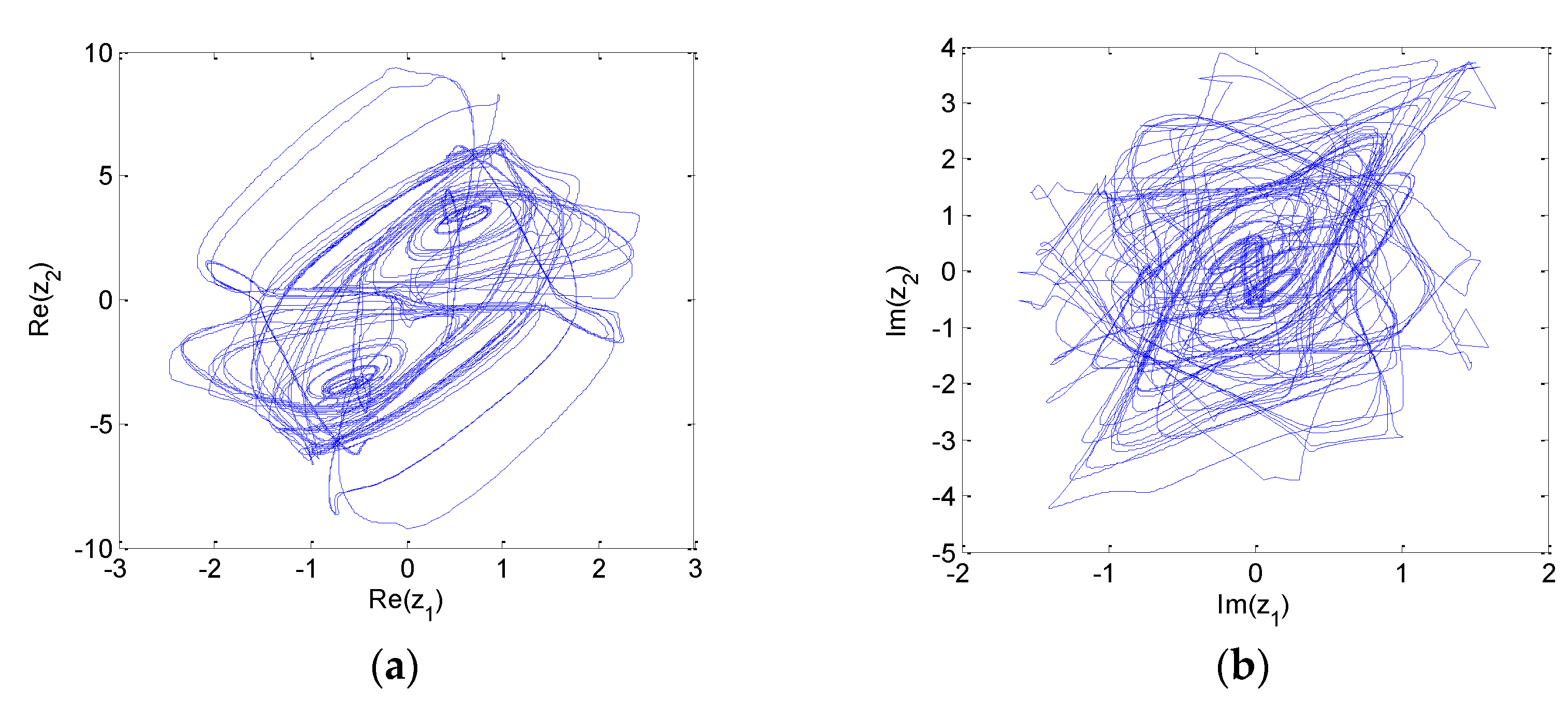
System (25) can exhibit chaotic behaviors, which can be called fractional-order complex-valued chaotic neural networks. While a11 = 2 + 0.1i and the other parameters are the same as above, the attractor trajectory with the initial condition is shown in Figure 2. The state trajectory is shown in Figure 3.
Let system (25) be the driving system and assume that the parameters are unknown, then the response FOCVCNNs are given as follows:
where are estimated values of , respectively and are controllers. The controllers and the update laws are selected as Equations (14)–(18). The following initial conditions are chosen:
, and , .
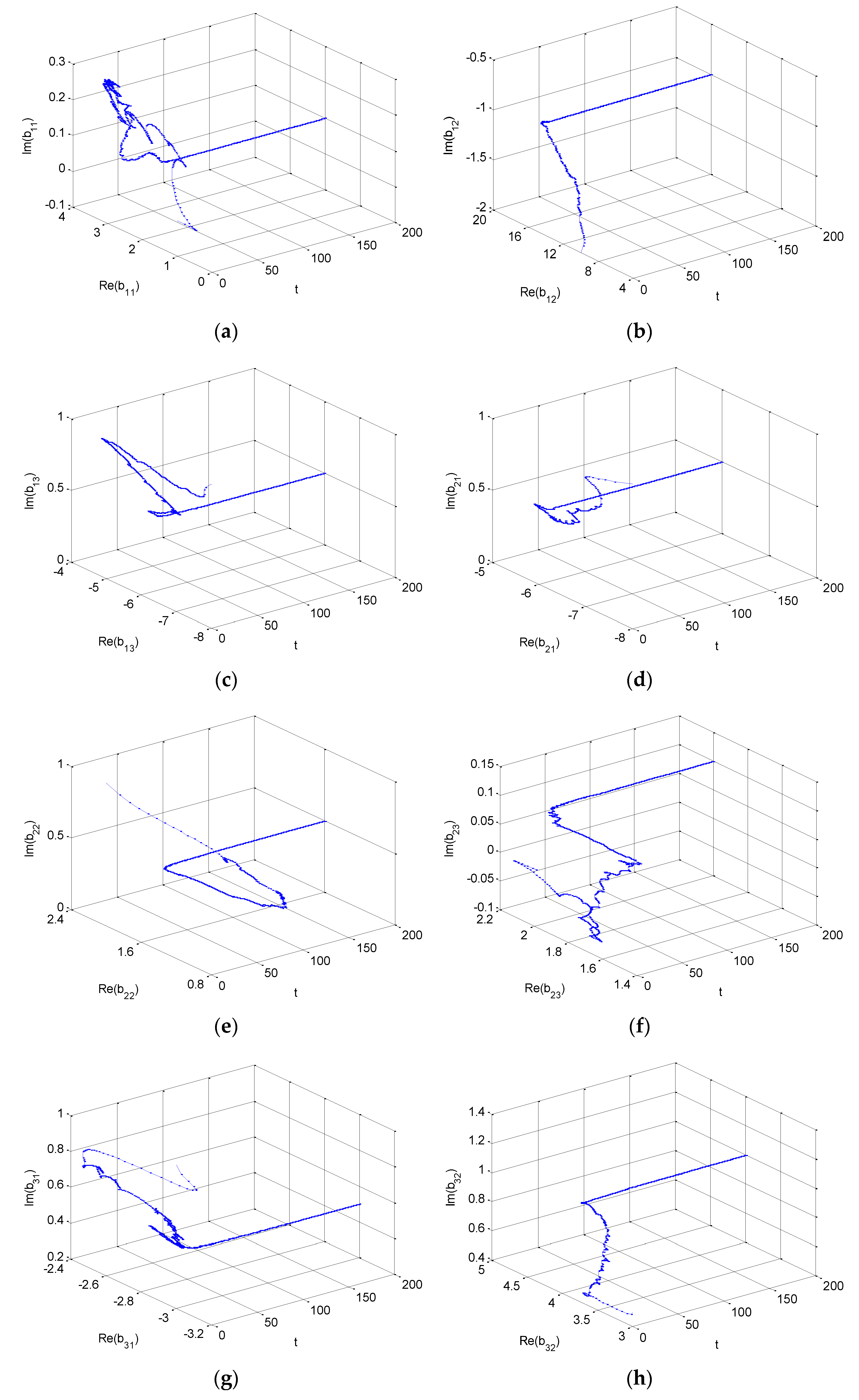
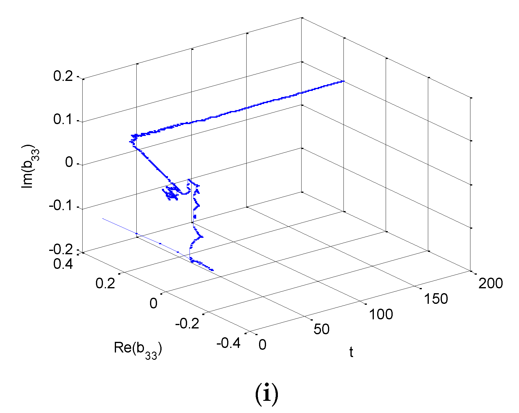
Two FOCVCNNs can achieve synchronization and the parameters are identified, as shown in Figure 4 and Figure 5. Figure 4 shows that the above two pairs of FOCVCNNs achieve asymptotic synchronization through the adaptive controller and adaptive update laws. Figure 5 indicates that all the unknown parameters of the driving system are identified.
It is shown that with this approach one can rapidly achieve global synchronization of these networks, while dynamically identifying all the unknown parameters. Additionally, this method is quite robust against noise effects.
Example 2.
To further illustrate the effectiveness and wider application of the proposed scheme, a higher dimensional FOCVNN is considered described by the following equation:
If is selected, then:
, , , , then system (27) can exhibit chaotic behaviors. The attractor trajectory is shown in Figure 6. The state trajectory is shown in Figure 7.
Taking system (27) as the driving system and assuming that the coefficients are unknown, the corresponding controlled response system is as follows:
where are estimated values of and are controllers. Let the system errors be . The controllers and the update laws are selected as Equations (14)–(18), and the initial conditions are chosen as follows:
The simulation results are shown in Figure 8 and Figure 9. Figure 8 shows that two pairs of high-dimensional FOCVCNNs achieve asymptotic synchronization through the adaptive controllers and adaptive update laws. Figure 9 indicates that all the unknown parameters of the driving system (27) are identified.
It is not difficult to see from Example 2 that the research results of this paper can be easily extended to the synchronization and parameter identification for high-dimensional FOCVCNNs. Meanwhile, the synchronization control and parameter identification schemes proposed in this paper have very loose conditions, which make them easy to implement in practical applications. In addition, the synchronization control strategies are quite robust to external disturbances.
5. Conclusions
This paper focuses on the synchronization and parameter identification of fractional-order complex-valued chaotic neural networks (FOCVCNNs) with time-delay and unknown complex parameters. Using the complex-valued inequalities of fractional derivatives and stability theory of fractional-order complex-valued systems, the adaptive controllers and complex update laws for synchronizing these systems are proposed. The proposed synchronization scheme preserves the complex nature of FOCVCNNs. Not only a new method for analyzing FOCVCNNs with time-delay and unknown complex parameters is provided here, but also a sensible decrease of the computational and analytical complexity.
Author Contributions
Conceptualization, M.L.; methodology, R.Z. and M.L.; software, R.Z.; validation, S.Y.; writing—review and editing, M.L. and R.Z.; supervision, S.Y. All authors have read and agreed to the published version of the manuscript.
Funding
The work of S.Y. was supported by the Natural Science Foundation of Hebei province, China (No. A2015205161), and the work of R.Z. was supported by the Science and technology support program of Xingtai, China (No. 2019ZC054).
Conflicts of Interest
The authors declare no conflict of interest.
References
- Nitta, T. Orthogonality of decision boundaries of complex-valued neural networks. Neural Comput. 2004, 16, 73–97. [Google Scholar] [CrossRef]
- Hirose, A. Complex-Valued Neural Networks: Theories and Applications; World Scientific Publishing Company: Singapore, 2003. [Google Scholar] [CrossRef] [Green Version]
- Tanak, G.; Aihara, K. Complex-valued multistate associative memory with nonlinear multilevel functions for gray-level image reconstruction. IEEE Trans. Neural Netw. 2009, 20, 1463–1473. [Google Scholar] [CrossRef]
- Amin, M.F.; Murase, K. Single-layered complex-valued neural network for real-valued classification problems. Neurocomputing 2009, 72, 945–955. [Google Scholar] [CrossRef] [Green Version]
- Rao, V.S.H.; Murthy, G. Global dynamics of a class of complex valued neural networks. Int. J. Neural Syst. 2008, 18, 165–171. [Google Scholar]
- Zhou, W.; Zurada, J.M. Discrete-time recurrent neural networks with complex-valued linear threshold neurons. IEEE Trans. Circuits Syst. II Express Briefs 2009, 56, 669–673. [Google Scholar] [CrossRef]
- Duan, C.; Song, Q. Boundedness and stability for discrete-time delayed neural network with complex-valued linear threshold neurons. Discret. Dyn. Nat. Soc. 2010, 19, 368–379. [Google Scholar] [CrossRef]
- Bohner, M.; Rao, V.S.H.; Sanyal, S. Global stability of complex-valued neural networks on time scales. Differ. Equ. Dyn. Syst. 2011, 19, 3–11. [Google Scholar] [CrossRef]
- Zeng, X.; Li, C.; Huang, T.; He, X. Stability analysis of complex-valued impulsive systems with time delay. Appl. Math. Comput. 2015, 256, 75–82. [Google Scholar] [CrossRef]
- Bao, H.; Park, J.H.; Cao, J. Synchronization of fractional-order complex-valued neural networks with time delay. Neural Netw. 2016, 81, 16–28. [Google Scholar] [CrossRef] [PubMed]
- Zhou, B.; Song, Q. Boundedness and complete stability of complex-valued neural networks with time delay. IEEE Trans. Neural Netw. Learn. Syst. 2013, 24, 1227–1238. [Google Scholar] [CrossRef] [PubMed]
- Huang, Y.; Zhang, H.; Wang, Z. Multistability of complex-valued recurrent neural networks with real-imaginary-type activation functions. Appl. Math. Comput. 2014, 229, 187–200. [Google Scholar] [CrossRef]
- Li, L.; Wang, Z.; Li, Y.; Shen, H.; Lu, J. Hopf bifurcation analysis of a complex-valued neural network model with discrete and distributed delays. Appl. Math. Comput. 2018, 330, 152–169. [Google Scholar] [CrossRef]
- Zhang, Z.; Lin, C.; Chen, B. Global stability criterion for delayed complex-valued recurrent neural networks. IEEE Trans. Neural Netw. Learn. Syst. 2014, 25, 1704–1708. [Google Scholar] [CrossRef]
- Hu, J.; Wang, J. Global stability of complex-valued recurrent neural networks with time-delays. IEEE Trans. Neural Netw. Learn. Syst. 2012, 23, 853–865. [Google Scholar] [CrossRef] [PubMed]
- Xu, X.; Zhang, J.; Shi, J. Exponential stability of complex-valued neural networks with mixed delays. Neurocomputing 2014, 128, 483–490. [Google Scholar] [CrossRef]
- Wan, P.; Jian, J. Global Mittag-Leffler boundedness for fractional-order complex-valued Cohen-Grossberg neural networks. Neural Process. Lett. 2019, 49, 121–139. [Google Scholar] [CrossRef]
- Yang, X.; Li, C.; Huang, T.; Song, Q.; Huang, J. Synchronization of fractional-order memristor-based complex-valued neural networks with uncertain parameters and time delays. Chaos Soliton Fractal 2018, 110, 105–123. [Google Scholar] [CrossRef]
- Lee, D.-L.; Wang, W.-J. A multivalued bidirectional associative memory operating on a complex domain. Neural Netw. 1998, 11, 1623–1635. [Google Scholar] [CrossRef]
- Bao, H.; Cao, J. Projective synchronization of fractional-order memristor-based neural networks. Neural Netw. 2015, 63, 1–9. [Google Scholar] [CrossRef]
- Bao, H.; Park, J.; Cao, J. Adaptive synchronization of fractional-order memristor-based neural networks with time delay. Nonlinear Dyn. 2015, 82, 1343–1354. [Google Scholar] [CrossRef]
- Chen, J.; Zeng, Z.; Jiang, P. Global Mittag–Leffler stability and synchronization of memristor-based fractional-order neural networks. Neural Netw. 2014, 51, 1–8. [Google Scholar] [CrossRef]
- Yang, X.; Li, C.; Song, Q.; Huang, T.; Chen, X. Mittag–Leffler stability analysis on variable-time impulsive fractional-order neural networks. Neurocomputing 2016, 207, 276–286. [Google Scholar] [CrossRef]
- Ding, Z.; Shen, Y.; Wang, L. Global Mittag–Leffler synchronization of fractional-order neural networks with discontinuous activations. Neural Netw. 2016, 73, 77–85. [Google Scholar] [CrossRef] [PubMed]
- Velmurugana, G.; Rakkiyappana, R.; Vembarasan, V.; Cao, J.; Alsaedi, A. Dissipativity and stability analysis of fractional-order complex-valued neural networks with time delay. Neural Netw. 2016, 86, 42–53. [Google Scholar] [CrossRef] [PubMed]
- Zhang, L.; Song, Q.K.; Zhao, Z.J. Stability analysis of fractional-order complex-valued neural networks with both leakage and discrete delays. Appl. Math. Comput. 2017, 298, 296–309. [Google Scholar] [CrossRef]
- Wang, L.; Song, Q.; Liu, Y.; Zhao, Z.; Alsaadi, F.E. Global asymptotic stability of impulsive fractional-order complex-valued neural networks with time delay. Neurocomputing 2017, 243, 49–59. [Google Scholar] [CrossRef]
- Rakkiyappan, R.; Velmurugan, G.; Cao, J. Stability analysis of fractional-order complex-valued neural networks with time delays. Chaos Solitons Fractals 2015, 78, 297–316. [Google Scholar] [CrossRef]
- Rakkiyappan, R.; Velmurugan, G.; Cao, J. Finite-time stability analysis of fractional-order complex-valued memristor-based neural networks with time delays. Nonlinear Dyn. 2014, 78, 2823–2836. [Google Scholar] [CrossRef]
- Chang, W.; Zhu, S.; Li, J.; Sun, K. Global Mittag–Leffler stabilization of fractional-order complex-valued memristive neural networks. Appl. Math. Comput. 2018, 338, 346–362. [Google Scholar] [CrossRef]
- Zhang, Y.; Deng, S. Finite-time projective synchronization of fractional-order complex-valued memristor-based neural networks with delay. Chaos Solitons Fractals 2019, 128, 176–190. [Google Scholar] [CrossRef]
- Li, L.; Wang, Z.; Lu, J.; Li, Y. Adaptive Synchronization of Fractional-Order Complex-Valued Neural Networks with Discrete and Distributed Delays. Entropy 2018, 20, 124. [Google Scholar] [CrossRef] [PubMed] [Green Version]
- Niamsup, P.; Botmart, T.; Weera, W. Modified function projective synchronization of complex dynamical networks with mixed time-varying and asymmetric coupling delays via new hybrid pinning adaptive control. Adv. Differ. Equ. 2017, 1, 1–31. [Google Scholar] [CrossRef] [Green Version]
- Chartbupapan, W.; Bagdasar, O.; Mukdasai, K. A novel delay-dependent asymptotic stability conditions for differential and Riemann-Liouville fractional differential neutral systems with constant delays and nonlinear perturbation. Mathematics 2020, 8, 82. [Google Scholar] [CrossRef] [Green Version]
- Dai, X.; Li, X.; Gutiérreze, R.; Guo, H. Explosive synchronization in populations of cooperative and competitive oscillators. Chaos Solitons Fractals 2020, 132, 109589. [Google Scholar] [CrossRef]
- Dai, X.; Li, X.; Jia, D.; Perc, M.; Manshour, P.; Wang, Z.; Boccaletti, S. Discontinuous Transitions and Rhythmic States in the D-Dimensional Kuramoto Model Induced by a Positive Feedback with the Global Order Parameter. Phys. Rev. Lett. 2020, 125, 194101. [Google Scholar] [CrossRef]
- Arslan, E.; Narayanan, G.; Ali, M.S.; Arik, S.; Saroha, M. Controller design for finite-time and fixed-time stabilization of fractional-order memristive complex-valued BAM neural networks with uncertain parameters and time-varying delays. Neural Netw. 2020, 130, 60–74. [Google Scholar] [CrossRef] [PubMed]
- Zhang, R.X.; Liu, Y.L. A new Barbalat’s lemma and Lyapunov stability theorem for fractional order systems. In Proceedings of the 29th Chinese control and decision conference (CCDC), Chongqing, China, 28–30 May 2017; pp. 3676–3681. [Google Scholar]
- Zhang, R.X.; Liu, Y.L.; Yang, S.P. Adaptive synchronization of fractional-order complex chaotic system with unknown complex parameters. Entropy 2019, 21, 207. [Google Scholar] [CrossRef] [Green Version]
- Zhang, R.X.; Feng, S.W.; Yang, S.P. Complex Modified Projective Synchronization of Fractional-order Complex-Variable Chaotic System with Unknown Complex Parameters. Entropy 2019, 21, 407. [Google Scholar] [CrossRef] [Green Version]
- Podlubny, I. Fractional Differential Equations; Academic Press: San Diego, CA, USA, 1999; Available online: https://0-www-sciencedirect-com.brum.beds.ac.uk/bookseries/mathematics-in-science-and-engineering/vol/198/suppl/C (accessed on 6 October 2021).
- Quan, X.; Zhuang, S.; Liu, S.; Xiao, J. Decentralized adaptive coupling synchronization of fractional-order complex-variable dynamical networks. Neurocomputing 2016, 186C, 119–126. [Google Scholar] [CrossRef]
- Li, H.L.; Hu, C.; Cao, J.D. Quasi-projective and complete synchronization of fractional-order complex-valued neural networks with time delays. Neural Netw. 2019, 118, 102–109. [Google Scholar] [CrossRef]
- Wu, Z.Y.; Chen, G.R.; Fu, X.C. Synchronization of a network coupled with complex-variable chaotic systems. Chaos Interdiscip. J. Nonlinear Sci. 2012, 22, 023127. [Google Scholar] [CrossRef] [PubMed]
- Kai, D.; Ford, D.J.; Freed, A.D. A predictor-corrector approach for the numerical solution of fractional differential equations. Nonlinear Dyn. 2002, 29, 3–22. [Google Scholar] [CrossRef]
- Gu, Y.; Yu, Y.; Wang, H. Synchronization-based parameter estimation of fractional-order neural networks. Phys. A Stat. Mech. Appl. 2017, 483, 351–361. [Google Scholar] [CrossRef]
- Wolf, A.; Swift, J.B.; Swinney, H.L.; Vastano, J.A. Determining Lyapunov exponents from a time series. Phys. D Nonlinear Phenom. 1985, 16, 285–317. [Google Scholar] [CrossRef] [Green Version]
Figure 1.
Dynamic behaviors of fractional-order complex-valued chaotic neural networks (FOCVCNNs) (25) with : (a) maximal Lyapunov exponent, (b) bifurcation diagram.
Figure 1.
Dynamic behaviors of fractional-order complex-valued chaotic neural networks (FOCVCNNs) (25) with : (a) maximal Lyapunov exponent, (b) bifurcation diagram.

Figure 2.
Chaotic attractors of FOCVCNNs (25) with , and fractional-order : (a) (b) .

Figure 3.
The state trajectories of FOCVCNNs with , and fractional-order , t is the time: (a) , (b) .
Figure 3.
The state trajectories of FOCVCNNs with , and fractional-order , t is the time: (a) , (b) .

Figure 4.
Synchronization errors of FOCVCNNs (25) and (26): (a) , (b) .

Figure 5.
Estimated complex parameters of FOCVCNNs (26): (a) , (b) (c) (d) (e) (f) (g) (h) .

Figure 6.
Chaotic attractors of FOCVCNNs (27): (a) , (b) , (c) , (d) .

Figure 7.
The state trajectories of FOCVCNNs (27): (a) , (b) .

Figure 8.
Synchronization errors of FOCVCNNs (27) and (28): (a) , (b) , (c) .

Figure 9.
Estimated complex parameters of FOCVCNNs (28): (a) , (b) , (c) (d) (e) (f) , (g) , (h) , (i) .
Figure 9.
Estimated complex parameters of FOCVCNNs (28): (a) , (b) , (c) (d) (e) (f) , (g) , (h) , (i) .


Publisher’s Note: MDPI stays neutral with regard to jurisdictional claims in published maps and institutional affiliations. |
© 2021 by the authors. Licensee MDPI, Basel, Switzerland. This article is an open access article distributed under the terms and conditions of the Creative Commons Attribution (CC BY) license (https://creativecommons.org/licenses/by/4.0/).
Share and Cite
MDPI and ACS Style
Li, M.; Zhang, R.; Yang, S. Adaptive Synchronization of Fractional-Order Complex-Valued Chaotic Neural Networks with Time-Delay and Unknown Parameters. Physics 2021, 3, 924-939. https://0-doi-org.brum.beds.ac.uk/10.3390/physics3040058
AMA Style
Li M, Zhang R, Yang S. Adaptive Synchronization of Fractional-Order Complex-Valued Chaotic Neural Networks with Time-Delay and Unknown Parameters. Physics. 2021; 3(4):924-939. https://0-doi-org.brum.beds.ac.uk/10.3390/physics3040058
Chicago/Turabian StyleLi, Mei, Ruoxun Zhang, and Shiping Yang. 2021. "Adaptive Synchronization of Fractional-Order Complex-Valued Chaotic Neural Networks with Time-Delay and Unknown Parameters" Physics 3, no. 4: 924-939. https://0-doi-org.brum.beds.ac.uk/10.3390/physics3040058