Some Features of the Direct and Inverse Double-Compton Effect as Applied to Astrophysics


1
Special Astrophysical Observatory, St. Petersburg Branch, Russian Academy of Sciences, 196140 St. Petersburg, Russia
2
Department of Physics, St. Petersburg State University, Petrodvorets, Oulianovskaya 1, 198504 St. Petersburg, Russia
*
Author to whom correspondence should be addressed.
Physics 2021, 3(4), 1167-1174; https://0-doi-org.brum.beds.ac.uk/10.3390/physics3040074
Submission received: 2 September 2021
/
Revised: 22 November 2021
/
Accepted: 22 November 2021
/
Published: 29 November 2021
(This article belongs to the Special Issue Light on Dark Worlds—A Themed Issue in Honor of Professor Maxim Yu. Khlopov on the Occasion of His 70th Birthday)
Abstract
:In the present paper, the process of inverse double-Compton (IDC) scattering is considered in the context of astrophysical applications. It is assumed that the two hard X-ray photons emitted from an astrophysical source are scattered on a free electron and converted into a single soft photon of optical range. Using the QED S-matrix formalism for the derivation of a cross-section of direct double-Compton (DDC) scattering and assuming detailed balance conditions, an analytical expression for the cross-section of the IDC process is presented. It is shown that at fixed energies of incident photons, the inverse cross-section has no infrared divergences, and its behavior is completely defined by the spectral characteristics of the photon source itself, in particular by the finite interaction time of radiation with an electron. Thus, even for the direct process, the problem of resolving infrared divergence actually refers to a real physical source of radiation in which photons are never actually plane waves. As a result, the physical frequency profile of the scattered radiation for DDC as well as for IDC processes is a function of both the intensity and line shape of the incident photon field.
The object of this paper is to give an expression for the inverse double-Compton effect (IDC), i.e., the third-order process in which two hard photons colliding with a free electron give rise to one scattered soft photon. The interest in such calculations lies in the fact that, though the cross-section for this process is small in comparison with ordinary Compton scattering, nevertheless, the high-intensity X-ray photons in the vicinity of astrophysical sources allow a possible study of these phenomena.
The ordinary direct double-Compton scattering has been repeatedly considered by many authors [1,2,3,4]. The exact relativistic expressions for the differential cross-section of the DC process accounting for angular correlations were obtained in [5] within the quantum electrodynamics (QED) formalism of the S-matrix. Various proposals for laboratory studies of the double-Compton effect have also been actively discussed in recent decades [6,7,8]. In addition, astrophysical applications are also of particular interest when describing the spectral features of various astrophysical sources and comparing them with ground-based or satellite observations [9].
The inverse double-Compton scattering is also of particular importance. Under astrophysical conditions, the IDC can be important for objects with a very high density of photons (for example, X-ray sources) or the in the early universe at a high intensity of the CMB. In these cases, the intensity of the generated high-frequency Raman radiation can be noticeable. For example, in the presence of a powerful line in the spectrum of the X-ray shell, in the observed spectrum, there will be an admixture of a line with a doubled energy, which cannot be identified with any chemical element. The importance of taking this effect into account is determined by the accuracy with which it is necessary to describe the physical parameters of the source and to avoid false identifications and estimates. Processes of this kind in various astronomical applications have been considered earlier [10]. In particular, in [10,11], the inverse processes included in the equations of balance and radiation transfer were expressed through direct ones, following the principle of detailed balance. However, as it is shown below, the forward process has divergence in the infrared region that is absent in the reverse process if one performs direct calculations.
When considering the direct double-Compton effect, there is some subtle effect of a fundamental nature—a feature of the formation of the infrared (low-frequency) end of the spectrum of the resulting photons—the so-called infrared catastrophe [11]. In the literature, there are a large number of versions of the solution to this problem [5,12]. To consistently cure the issue, the DC process has to be treated together with the next-to-leading-order (NLO) radiative corrections to the Compton process [11,13]. In this context, one is usually interested in the total Compton scattering cross-section at fine structure-constant order . The NLO corrections display a logarithmic divergence, which can be shown to cancel with the corresponding DC one. Employing a regularization—introducing a photon mass in the standard approach [13]—in the calculation of both cross-sections and summing the two, the dependence on the regularization parameters drops out, leaving a finite radiative correction at order . The drawback of this approach is that the radiative correction cross-section now depends on the energy resolution of the experiment, . The argument to justify summing the two processes is that below some , the experiment is unable to distinguish contributions from virtual photon emission, relevant to the computation of the NLO correction, and from real photon emission by DC. Adding all contributions to the total CS scattering cross-section, it was found that the correction can exceed the naive level at sufficiently high energies [14]. It is should be noted that direct and inverse process were recently studied in laboratory conditions [15]. In [15], it was shown that measured direct double-Compton (DDC) and IDC cross-sections are of comparable magnitudes and agree with theoretical predictions. From this, it can be concluded that it is important to take into account both processes in problems related to radiation transfer.
However, all of the regularization procedures are related to the consideration of the final state of the system [13]. In this paper, a different physical approach is proposed for solving this problem based on the analysis of the input photon—taking into account its finiteness in time. Indeed, the standard consideration assumes that the incident photon is taken in the form of a plane wave infinite in time and space [16,17,18,19]. Only in this case, there is the possibility to form an arbitrarily low-frequency photon at the end of the process. However, in reality, there are no such waves in nature. There are only real photons, which are formed by some radiation mechanism during a finite time interval [20]. As a result, the scattering of such a photon by an electron leads to a finite spectrum that is completely finite in the entire frequency range. From the point of view of observational astrophysics, this provides an alternative way to determine the parameters of an incident photon from the spectrum of the low-frequency wing. Thus, we obtain a new independent channel of information about the mechanism of radiation formation in the source.
Below, it is shown that in real physical conditions, the problem of eliminating the infrared divergence in the cross-section of the direct process refers to the finite interaction time of radiation with an electron, which can be introduced at least phenomenologically within the QED formalism. For these purposes, first, the cross-section of the reverse process is considered in the context of its astrophysical application. it is assumed that two photons emitted in the vicinity of some object are scattered on a free electron and convert into a single photon . It is also assumed that this process, along with a direct one, can leave significant distortions in the spectrum of some astrophysical source in the vicinity of which the events of collisions of photons with an electron gas occur. The characteristic behavior of the cross-section of the inverse double-Compton scattering is derived within the framework of the rigorous QED approach.
To begin with, let us recall a brief derivation of the scattering cross-section of the direct process [21]. Following [22], the DDC is described by the third-order S-matrix element (here and below, relativistic units , are used, where ℏ is the reduced Planck constant, c is the speed of light, and e is the electron charge; the electron mass is written explicitly):
where , are the four-vectors of initial and final electron momenta, respectively; is the four-vector of incident photon with frequency and wave vector , and are the four-vectors of two outgoing photons, and is the Feynman amplitude of the process:
Here, is the Dirac spinor for free electron with its Dirac adjoint defined as , () are the Dirac matrices, and is the polarization four-vector of a photon k. The contraction of matrices with four-vector a is given by .
The transition rate per unit time to one defined state can be found according to the definition:
where is the observation time and V is the phase volume. Since we are interested in a transition rate to a group of final states with momenta in the intervals , , and , Equation (3) has to be multiplied by the number of these states, which is:
With the chosen normalization for the states, the volume V contains one scattering center and the incident photon flux is [23]. Then, the corresponding differential DDC cross-section can be found as follows:
Integration over final electron momenta in Equation (5) can be written in a four-dimensional form with the use of the equality [17]:
where and is the Heaviside step function. Finally, performing integration over with the use of delta function properties, one finds [5,7]:
Let us now specialize to a reference frame where the electron is initially at rest, i.e., and . Then, the argument of the delta function in Equation (7) becomes:
where is the angle between vectors and , is the angle between vectors and , and is the angle between vectors and . Here, , and are assumed. Then, the energy conservation law has the form:
Taking into account that in spherical coordinates (where and , are the spherical angles of vector ), performing integration over in Equation (7) with the use of the equality:
and summing over the photon polarizations and electron spin in the initial and final states, one finds:
where:
Summation in Equation (11) and algebra with Dirac matrices can be performed in a fully analytical way with the use of the FeynCalc software [24,25].
To describe the stimulated DDC cross-section, magnitude Equation (2) has to be also multiplied by the factor , where is the number of photons with a wave vector and polarization . In this case, the corresponding flux of incident photons is [23]. Then, the number of incident photons vanishes in the cross-section. If the intensity of the radiation is known, then can be obtained with the use of the following relation:
It is known that DDC cross-section Equation (11) has infrared divergence of the type [5]. In [13], it was shown that accounting of QED radiative corrections leads to the natural cut-off of the lower limit of frequency , which can be attributed to the minimal resolution of the detector in the experiment. Below, it is shown that for the inverse process, the divergence is moved from the problem of the resolution detector of photons in final states to the source of initial photons.
Using the definition for transition rate Equation (2), one can write the equation for the cross-section of the inverse double-Compton scattering (IDC) as follows:
In the reference frame where the electron is initially at rest (), the frequency of outgoing photon takes the form:
The scalar products of the four-vectors included in Equation (15) are given by the following equalities: , , , , , , , , , and
Then, integration over , and summation over the photon polarizations and electron spin in the initial and final states gives:
where:
The magnitude for the inverse process in Equation (17) differs from the direct one only in the use of a different expression for the energy conservation law (see Equations (9) and (15)) and by the replacement , , and .
Following [5], one can consider the particular case when particles are moving nearly in the forward direction. Then, introducing notations , , and , one finds:
where , , and are assumed to be small, . As well as the DDC cross-section, Equation (18) vanishes for scattering in the forward direction, i.e., when (i.e., in Equation (18)). From Equation (18), its is seen that the IDC scattering cross-section (as well as the DDC) is the order smaller than single-Compton scattering.
The dependence on angles , , in Equation (18) can be expressed in terms of spherical angles (, ), (, ), and (, ) with the use of relations:
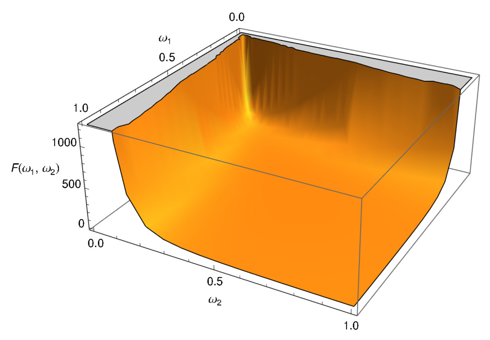
For a particular case, when two incident photons and are propagating parallel with each other, it is convenient to choose the z-axis of the spherical coordinate system along this direction. Then, setting , and performing integration over in the Equations (18), one finds:
The function is drawn in Figure 1. To note is that , are the input parameters of the cross-section, and they never turn to zero for the real source of photons.
For an incident photon with equal energies, , Equation (18) turns into:
In the case the IDC, the accounting of the stimulated scattering can be taken into account by multiplying the magnitude of the process by the factor and dividing by the photon flux [23]. Assuming that for a direct process, there is a system of electron + photon field with photons, the following relation between the transition rates of direct and inverse processes can be found [23,26]:
The equation above was used in [10,11] when the evolution of the photon occupation number was considered. Let us note that the behavior of the left side of Equation (25) in the infrared region depends on the ratio of the photon occupation numbers on the right side of this equation. Since all in Equation (25) are defined by the properties of a real source, one can conclude that the divergence problem is actually solved by the constraints on the source.
Performing the analytical evaluation of cross-section Equation (16), we find that the cross-section of the IDC has no infrared divergence in variable , and as a result, the total cross-section becomes finite in contrast to the direct process. However, there is another divergence of the type (a and b are some integers ) that depends now only on input parameters. The cross-section becomes infinite for the unphysical situation when two incident photons have zero energy. Since the real source of photons always has a finite width, the frequencies and in Equation (16) are also finite. Similarly, for a direct process, the solution to the problem of infrared divergence can be resolved by taking into account the fact that, under the real physical conditions, the photon wave function cannot be described by a plane wave. As a result, the physical frequency profile of the scattered radiation for direct, as well as inverse DC processes is a function of both the intensity and line shape of the incident photon field [20]. The monochromatic limit, while it may exist as a mathematical exercise, is not germane to the physical scattering problem. The shape and extent of the external field are fundamental aspects of the problem.
Thus, one can that the problem of divergence can be solved not only by imposing restrictions on the detector and its resolution, but also by taking into account the spectral characteristics of the source itself, in particular taking into account the finite interaction time of radiation with an electron. The latter circumstance for the theory of free particles can be taken into account phenomenologically by analogy with the quantum-mechanical description of photon scattering processes on atoms, where singular denominators are regularized by the introduction of atomic level widths [27,28,29]. Then, following [27], the infrared behavior of the DDC scattering can be naively regularized as follows:
where and is the interaction time of the incident photon with the electron. For the inverse process, there is no divergence, and such regularization is not needed. However, the introduction of in this case is also possible and should lead to the correct infrared asymptotic behavior when two incident photons are soft.
In conclusion, it must be added that with the sufficient intensity of an external astrophysical radiation source, the inverse process can also be of interest in the study and analysis of scattering spectra by electrons [11]. As shown in this study, the cross-section of the inverse process has no infrared features and is determined entirely by the spectral density of incident photons. We leave the application to the study of different astronomical situations for the future work. The presented calculations represent only the first step towards solving the complete problem of the radiation transfer equation, where incident photons interact with an electron for a finite period of time.
Author Contributions
Conceptualization, V.D.; investigation, T.Z. All authors have read and agreed to the published version of the manuscript.
Funding
The work was performed as part of the government contract of the SAO RAS approved by the Ministry of Science and Higher Education of the Russian Federation.
Conflicts of Interest
The authors declare no conflict of interest.
References
- Heitler, W. von; Nordheim, L. Über die wahrscheinlichkeit von mehrfachprozessen bei sehr hohen energieen. Physica 1934, 1, 1059–1072. [Google Scholar] [CrossRef]
- Eliezer, C.J. The application of quantum electrodynamics to multiple processes. Proc. R. Soc. Lond. Ser. A Math. Phys. Sci. 1946, 187, 210–219. [Google Scholar]
- Cavanagh, P.E. The double Compton effect. Phys. Rev. 1952, 87, 1131. [Google Scholar] [CrossRef]
- Levine, B.; Freund, I. Double quantum scattering of X rays. Opt. Commun. 1971, 3, 197–200. [Google Scholar] [CrossRef]
- Mandl, F.; Skyrme, T. The theory of the double-Compton effect. Proc. R. Soc. Lond. Ser. A Math. Phys. Sci. 1952, 215, 497–507. [Google Scholar] [CrossRef]
- Lotstedt, E.; Jentschura, U. Theoretical study of the Compton effect with correlated three-photon emission: From the differential cross section to high-energy triple-photon entanglement. Phys. Rev. A 2013, 87, 033401. [Google Scholar] [CrossRef] [Green Version]
- Lötstedt, E.; Jentschura, U.D. Nonperturbative treatment of double Compton backscattering in intense laser fields. Phys. Rev. Lett. 2009, 103, 110404. [Google Scholar] [CrossRef] [Green Version]
- Sherwin, J.A. Theoretical study of the double-Compton effect with twisted photons. Phys. Rev. A 2017, 95, 052101. [Google Scholar] [CrossRef]
- Chluba, J.; Sazonov, S.Y.; Sunyaev, R.A. The double-Compton emissivity in a mildly relativistic thermal plasma within the soft photon limit. Astron. Astrophys. 2007, 468, 785–795. [Google Scholar] [CrossRef] [Green Version]
- Lightman, A.P. Double Compton emission in radiation dominated thermal plasmas. Astrophys. J. 1981, 244, 392–405. [Google Scholar] [CrossRef]
- Ravenni, A.; Chluba, J. The double-Compton process in astrophysical plasmas. J. Cosmol. Astropart. Phys. 2020, 2020, 025. [Google Scholar] [CrossRef]
- Jauch, J.M.; Rohrlich, F. The Theory of Photons and Electrons. The Relativistic Quantum Field Theory of Charged Particles with Spin One-Half; Springer: Berlin/Heidelberg, Germany, 1976. [Google Scholar] [CrossRef]
- Brown, L.M.; Feynman, R.P. Radiative corrections to Compton scattering. Phys. Rev. 1952, 85, 231–244. [Google Scholar] [CrossRef]
- Mork, K.J. Radiative corrections. II. Compton effect. Phys. Rev. A 1971, 4, 917–927. [Google Scholar] [CrossRef]
- Sandhu, B.S.; Saddi, M.B.; Singh, B.; Ghumman, B.S. Scattering and absorption differential cross sections for double photon Compton scattering. Pramana 2001, 57, 733. [Google Scholar] [CrossRef]
- Akhiezer, A.I.; Berestetskii, V.B. Quantum Electrodynamics; Wiley-Interscience: New York, NY, USA, 1965. [Google Scholar]
- Bjorken, J.D.; Drell, S.D. Relativistic Quantum Mechanics; Mcgraw-Hill: New York, NY, USA, 1964. [Google Scholar]
- Landau, L.D.; Lifshitz, E.M. Quantum Mechanics: Non-Relativistic Theory; Pergamon Press Ltd.: Oxford, UK, 1965. [Google Scholar]
- Berestetskii, V.B.; Lifshits, E.M.; Pitaevskii, L.P. Quantum Electrodynamics; Pergamon Press Ltd.: Oxford, UK, 1982. [Google Scholar]
- Dawson, J.F.; Fried, Z. Plane-wave packets and their limitation in nonlinear compton scattering. Phys. Rev. D 1970, 1, 3363–3370. [Google Scholar] [CrossRef]
- Melrose, D.B. A classical counterpart to double-Compton scattering. Nuovo Cim. A 1972, 7, 669–686. [Google Scholar] [CrossRef]
- Mandl, F.; Shaw, G. Quantum Field Theory; John Wiley & Sons Inc.: Chichester, UK, 1984. [Google Scholar]
- Rapoport, L.; Zon, B.; Manakov, N. Theory of Multiphoton Processes in Atoms.; Atomizdat: Moscow, USSR, 1978. (In Russian) [Google Scholar]
- Mertig, R.; Böhm, M.; Denner, A. Feyn Calc—Computer-algebraic calculation of Feynman amplitudes. Comput. Phys. Commun. 1991, 64, 345–359. [Google Scholar] [CrossRef]
- Shtabovenko, V.; Mertig, R.; Orellana, F. New developments in FeynCalc 9.0. Comput. Phys. Commun. 2016, 207, 432–444. [Google Scholar] [CrossRef] [Green Version]
- Labzowsky, L.; Klimchitskaya, G.; Dmitriev, Y. Relativistic Effects in the Spectra of Atomic Systems; Institute of Physics Publishing: Philadephia, PA, USA, 1993. [Google Scholar]
- Low, F. Natural line shape. Phys. Rev. 1952, 88, 53. [Google Scholar] [CrossRef]
- Zalialiutdinov, T.A.; Solovyev, D.A.; Labzowsky, L.N.; Plunien, G. QED theory of multiphoton transitions in atoms and ions. Phys. Rep. 2018, 737, 1–84. [Google Scholar] [CrossRef]
- Andreev, O.Y.; Labzowsky, L.N.; Plunien, G.; Solovyev, D.A. QED theory of the spectral line profile and its applications to atoms and ions. Phys. Rep. 2008, 455, 135–246. [Google Scholar] [CrossRef]

Publisher’s Note: MDPI stays neutral with regard to jurisdictional claims in published maps and institutional affiliations. |
© 2021 by the authors. Licensee MDPI, Basel, Switzerland. This article is an open access article distributed under the terms and conditions of the Creative Commons Attribution (CC BY) license (https://creativecommons.org/licenses/by/4.0/).
Share and Cite
MDPI and ACS Style
Dubrovich, V.; Zalialiutdinov, T. Some Features of the Direct and Inverse Double-Compton Effect as Applied to Astrophysics. Physics 2021, 3, 1167-1174. https://0-doi-org.brum.beds.ac.uk/10.3390/physics3040074
AMA Style
Dubrovich V, Zalialiutdinov T. Some Features of the Direct and Inverse Double-Compton Effect as Applied to Astrophysics. Physics. 2021; 3(4):1167-1174. https://0-doi-org.brum.beds.ac.uk/10.3390/physics3040074
Chicago/Turabian StyleDubrovich, Viktor, and Timur Zalialiutdinov. 2021. "Some Features of the Direct and Inverse Double-Compton Effect as Applied to Astrophysics" Physics 3, no. 4: 1167-1174. https://0-doi-org.brum.beds.ac.uk/10.3390/physics3040074