
Linear and Nonlinear Plasma Processes in Ionospheric HF Heating


Department of Electrical and Computer Engineering, Tandon School of Engineering, New York University 5 MetroTech Center, Brooklyn, NY 11201, USA
Plasma 2021, 4(1), 108-144; https://0-doi-org.brum.beds.ac.uk/10.3390/plasma4010008
Submission received: 25 December 2020
/
Revised: 26 January 2021
/
Accepted: 19 February 2021
/
Published: 23 February 2021
Abstract
:Featured observations of high frequency (HF) heating experiments are first introduced; the uniqueness of each observation is presented; the likely cause and physical process of each observed phenomenon instigated by the HF heating are discussed. A special point in the observations, revealed through the ionograms, is the competition between the Langmuir parametric instability and upper hybrid parametric instability excited in the heating experiments and the impact of the natural cusp at foE (the peak plasma frequency of the ionospheric E region) on the competition. The ionograms also infer the generation of Langmuir and upper hybrid cavitons. Ray tracing theory is formulated. With and without the appearance of large-scale field-aligned density irregularities in the background ionosphere, ray trajectories of the ordinary mode (O-mode) and extraordinary mode (X-mode) sounding pulses are calculated numerically. The results explain the artificial Spread-F recorded by the digisondes in the heating experiments. Parametric instabilities, which are the directly relevant processes to achieve effective heating of the ionospheric F region, are formulated and analyzed. The threshold fields and growth rates of Langmuir and upper hybrid parametric instabilities are derived as the theoretical basis of many radar observations and electron-plasma wave interactions. Harmonic cyclotron resonance interaction processes between electrons and upper hybrid waves are introduced. Formulation and analysis are presented. The numerical results show that ultra-energetic electrons are generated. These electrons enhance airglow at 777.4 nm as well as cause ionization. Physical processes leading to the generation of artificial ionization layers are discussed. The nonlinear Schrodinger equation governing the nonlinear evolution of Langmuir waves and upper hybrid waves are derived and solved. The nonlinear periodic and solitary solutions of the equations are obtained. The localized Langmuir and upper hybrid waves generated by the HF heater form cavitons near the HF reflection layer and near the upper hybrid resonance layer, which induce bumps in the virtual height spread of the ionogram trace similar to that induced by the density cusp at E-F1 transition layer; the down-going Langmuir waves and upper hybrid waves evolve into nonlinear periodic waves propagating along the magnetic field, which backscatter incoherently the sounding pulses to cause downward virtual height spread.
1. Introduction
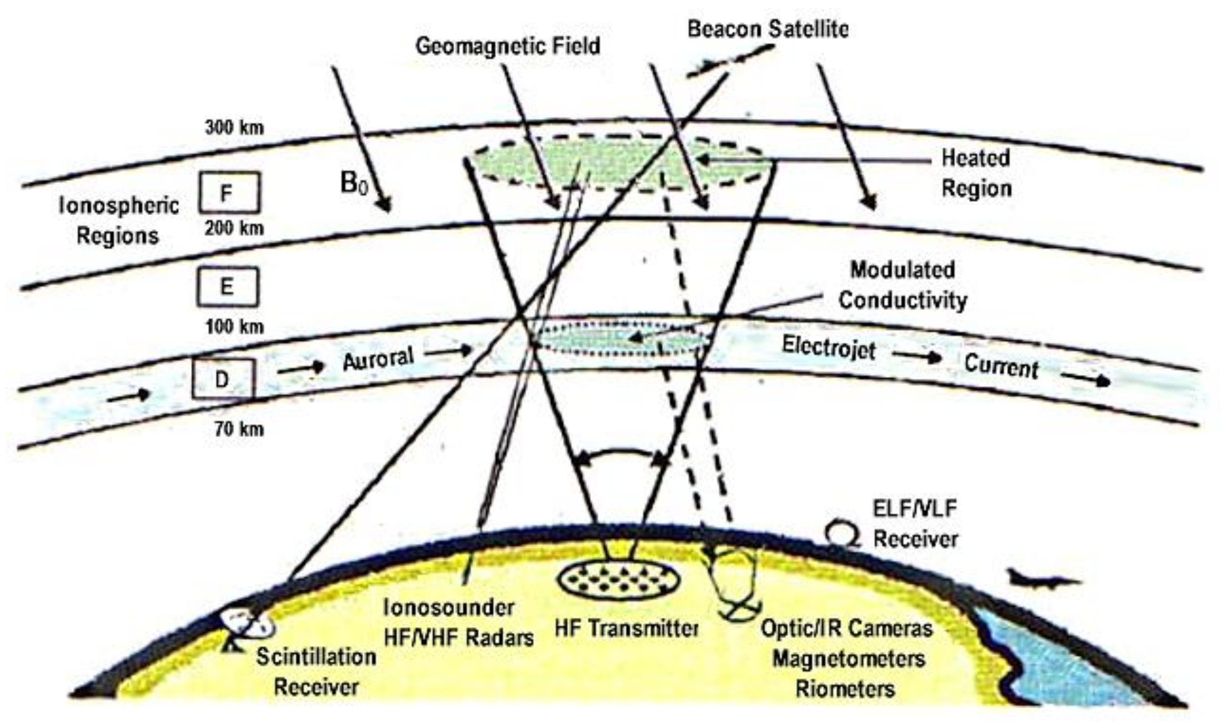
Using ionosphere as an unbounded plasma laboratory to study linear and nonlinear plasma processes, instigated by high frequency (HF) pump waves, has been a highly active research area over the past four decades [1,2,3]. Experiments were conducted by transmitting powerful HF waves from the ground to observe Ionospheric modification via remote-sensing instruments. A major facility has been built in Gakona, Alaska for conducting ionospheric heating experiments, as part of the High-Frequency Active Auroral Research Program (HAARP) [4]. The HAARP HF transmitting system has a rectangular planar array of 180 elements, which consist of a low band (2.8 to 7.6 MHz) and a high band (7.6 to 10 MHz) crossed dipole antenna in each element. Each crossed dipole radiates circularly polarized wave up to 20 kW, so that the HAARP HF transmitter radiates circularly polarized waves, in the frequency band from 2.8 MHz to 10 MHz, up to 3.6 MW. The antenna gain increases from 15 dB to 30 dB with an increase of the radiating frequency from 2.8 MHz to 10 MHz. An effective radiated power (ERP) up to 93 dBw (at 10 MHz) is available in heating experiments, which explore modification effects on the bottom-side of the ionosphere as illustrated in Figure 1. Through the observations of various heating induced phenomena presented in Section 2, considerable advances are toward the theory of wave–wave and wave–particle interactions.
Electromagnetic waves interact with charged particles; only electrons can effectively respond to the fast oscillation of the HF wave electric field. Through elastic and inelastic collisions with charged particles (mainly electrons), neutral particles can also be indirectly affected by the presence of HF waves. In D and E regions, electron–neutral collision frequency is higher than electron-electron and electron–ion collision frequencies. Although neutral particles can share considerable wave energy with charged particles and rapidly thermalize the indirectly absorbed wave energy, the background temperature elevation is small due to high neutral-particle density. Nevertheless, a long heating period in the daytime could still make an impact on the ionization balance, which involves the processes of (1) photoionization by the solar illumination, (2) electron-heating-caused reduction of the recombination coefficient, and (3) enhancement of the electron attachment to the oxygen molecules. Moreover, electrojet appeared in these regions can be modulated by intensity modulated HF heating waves to become a virtual antenna, which radiates ELF/VLF waves [5]. Applying an HF heating facility to establish an ionospheric virtual ELF/VLF transmitter for undersea communications is another focus of research.
However, most of the HF heating experiments were focused on the F region modification on the bottom side of the ionosphere, where the HF heating wave induces significant electron quiver motion in the region below and near the HF reflection height; parametric instabilities are excited to convert EM wave to plasma (ES) waves [6]. This is done by employing O-mode heating wave with frequency less than the maximum cutoff frequency (FoF2) of the ionosphere to confine the HF wave in the bottom side of the ionosphere. The excitation of parametric instabilities is essential because the collision (electron–electron and electron–ion) processes cannot efficiently absorb the electromagnetic (EM) wave energy delivered to the F region of the ionosphere, and a fast conversion of EM wave into electrostatic (ES) waves (via parametric instabilities) minimizes the loss of the heating power due to reflection back to the ground. The excited plasma waves interact with electrons as well as are interacting among themselves; as a result, new phenomena have been observed in the experiments, which are called for theoretical interpretations.
The present work is aimed at providing theoretical foundation for the understanding of experimental observations in active wave-ionosphere interaction and the underlying linear and nonlinear plasma processes. Among the experimental observations of various heating-induced phenomena, some of those featured are first described physically in Section 2. Theoretical formulations and analyses of the relevant linear and nonlinear mechanisms and processes are presented in Section 3, Section 4, Section 5, Section 6 and Section 7.
2. Featured Observations in HF Heating Experiments
2.1. HFPLs and HFILs
Monostatic backscatter radars record signals from incoherent and coherent backscattering, which are ascribed to the inhomogeneity of the background plasma and to the Bragg scattering by the plasma waves (electron plasma waves as well as ion plasma waves), respectively, and are used to monitor background plasma density variation and plasma wave intensity. A plasma wave scatters the radar signal to produce new signals , whose frequencies and wavevectors are imposed by the Bragg scattering (matching) conditions: and . Because , ; in the backscattering, . Thus, the plasma waves that backscatter radar signals have a wavelength half of that of the radar signal (i.e., propagate parallel or antiparallel to the radar signal, and produce frequency down-shifted (i.e., and upshifted (i.e., radar returns, respectively. The frequency spectrum of backscatter-radar returns is then offset by the radar frequency to present a distribution (with ∓ω) on both sides of the zero central frequency. The spectral lines on the negative side correspond to up-going plasma lines and those on the positive side correspond to down-going plasma lines.
In the unperturbed ionosphere, the spectral intensity of coherent backscatter lines is at noise level. On the other hand, in HF heating experiments transmitting O-mode heating waves , both up-going and down-going plasma lines and ion lines were recorded by backscatter radars. The offset (by the radar frequency) frequency spectrum, representing the electron plasma lines, contains discrete spectral peaks located at of the HF heating wave frequency and at frequencies downshifted from by , where 2 is an ion acoustic frequency and is the ion acoustic speed. These plasma lines were enhanced by the HF heating waves; thus, they are named “HF enhanced plasma lines (HFPLs)”. The spectral features suggest that HFPLs are correlated to oscillating two stream instability (OTSI), parametric decay instability (PDI), and Langmuir cascade. First, these parametric instabilities are only excited by the O mode HF heating waves. OTSI excites Langmuir waves together with non-oscillatory purely growing modes ; thus, it is revealed by the spectral peaks at the heater frequency in the distribution of the HFPLs. PDI decays the HF heating wave to Langmuir waves and ion acoustic waves . The wavevector of the HFPLs is , thus the spectral peaks have a downshifted frequency from the heating wave frequency by , i.e., located at . When the PDI excited Langmuir wave cascades to a new Langmuir wave and an ion acoustic wave , the frequency, , of the first cascade plasma line is downshifted from by about 6. In other words, Langmuir cascade lines in the HFPLs are separated by intervals about double the ion-acoustic frequency separating the OTSI line and the PDI line in the HFPLs. At HAARP, cascade lines were observed in lower heating power operation, but not observed in high power operation. Heating power depletion (pump depletion) by the upper-hybrid OTSI/PDI excited in the region below the Langmuir OTSI/PDI as well as the mode competition induced nonlinear-damping are suggested as the mechanisms, suppressing cascade enhanced HFPLs.
Likewise, the offset (by the radar frequency) frequency spectrum, representing the ion lines, contains discrete spectral peaks located at zero (i.e., at ) and at of the ion acoustic frequency, which represent non-oscillatory purely growing modes excited by the OTSI and ion acoustic modes excited by the PDI and Langmuir cascade, respectively. These ion lines were enhanced by the HF heater and thus named “HF enhanced ion lines (HFILs)”.
In Arecibo HF heating experiments, overshoot [7,8] of the intensity and down shifting [9,10] of the originating height in time of the HFPLs were observed. It is realized that the relevant parametric instabilities prefer to excite Langmuir waves along the geomagnetic field. On the other hand, the Langmuir waves ascribed to the HFPLs, which must have an oblique propagation angle of 40° at the Arecibo site, are not the preferred ones. Thus, these Langmuir waves are suppressed in time by those preferred ones having much larger growth rates (mode competition nonlinear damping). A spectral distribution of Langmuir waves, excited by the HF heater via parametric instabilities, interact with background electrons. The non-resonance interaction with bulk electrons (wave phase velocity is much larger than the electron velocity) in the velocity distribution broadens the distribution to have an equivalent temperature , where is the electron temperature of unperturbed background plasma and is the time average wave energy per electron. The matching height of the Langmuir wave decreases with the increase of the effective electron temperature, which is proportional to the total spectral intensity of the Langmuir waves.
Measurements also show asymmetry [11] of the HFPL distribution on the negative side (corresponding to up-going plasma lines) and on the positive side (down-going plasma lines). It is realized that the spectral intensity on the positive side of the HFPLs is ascribed to the excited down-going plasma waves as well as the excited up-going plasma waves after being reflected. Both OTSI and PDI were excited very close to the HF reflection height, and the reflected back plasma waves did not attenuate significantly when combining with the down-going plasma waves.
2.2. Competition between Langmuir PDI and Upper Hybrid PDI
Parametric instabilities excited in the HF heating experiments have been monitored by UHF/VHF radars [1,3], which receive return signals backscattered by the plasma waves. Because of the imposed Bragg backscattering conditions, the exploration of parametric instabilities by UHF/VHF backscatter radars in HF heating experiments is limited to HFPLs and HFILs, which do not represent the spectra of the plasma waves excited by parametric instabilities. Moreover, UHF/VHF radars do not detect magnetic field-aligned waves (i.e., wavevectors are closely perpendicular to the magnetic field), such as the upper and lower hybrid waves, because those waves do not backscatter radar pulses. On the other hand, the O-mode heating wave propagates through the upper hybrid resonance layer before reaching the reflection height in an over-dense ionosphere; thus, Langmuir and upper hybrid parametric instabilities can be excited simultaneously by a HF heating wave [12,13]. Langmuir and upper hybrid waves exert ponderomotive and thermal pressure forces on electrons [14,15], which induce nonlinear feedback on the waves. Thus, intense Langmuir and upper hybrid waves evolve to nonlinear waves, which have periodic and solitary envelopes; solitary waves press out local plasma in a self-consistent way to form cavitons [16,17].
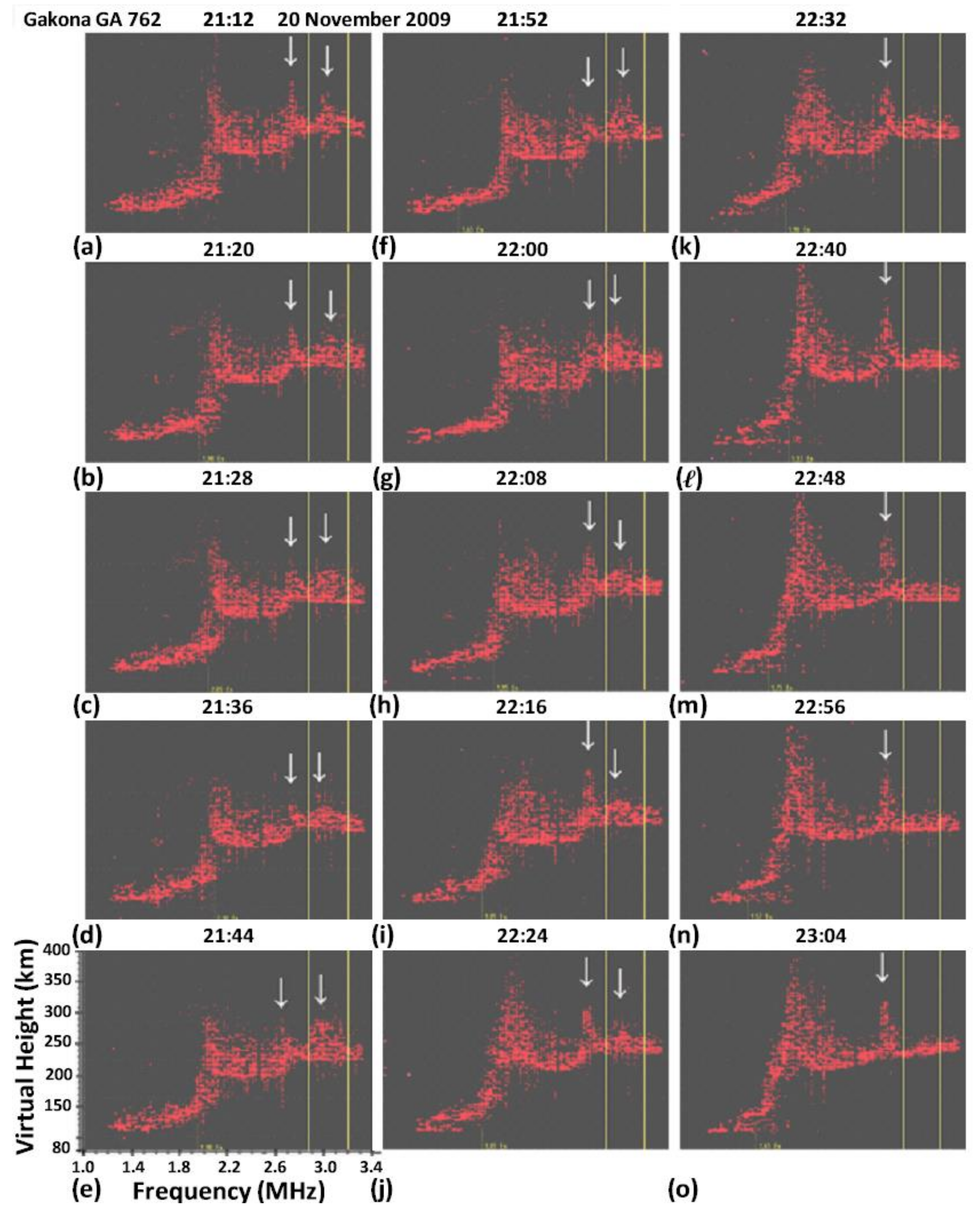
A digisonde [18] was used to explore Langmuir and upper hybrid parametric instabilities excited in the HF heating experiments. The experiment was conducted with 2 min on and 2 min off on 20 November 2009 from 21:00 to 23:04 UT. In the on period, the polarization of the heating wave was switched alternately with O mode and X mode. Echo spread with bump(s) occurs only after O mode heating. The spread was fading away in the subsequent off period and eliminated further by the X-mode heater. In essence, it was 2 min on and 6 min off. The Sun was above the HAARP horizon for the entire experiment period. Therefore, there was no precondition on the background plasma for each O mode heating period. The experimental observations of exciting Langmuir and upper hybrid waves were manifested by bumps in the virtual spread of the ionogram trace, which are located closely below the HF heater frequency and the upper hybrid resonance frequency [12,13]. The time development of bumps in the ionogram trace, which signifies the competition between Langmuir PDI and upper hybrid PDI, was observed [12,13]. This is demonstrated in a sequence of 15 ionograms, presented in Figure 2a–o. The echoes (red dots) in each ionogram were acquired at the beginning of the moment when the O mode heater turned off.
The results show the time change of the virtual height spread as well as the development of bumps next to the HF reflection layer and upper hybrid resonance layer. In Figure 2a–j, bumps, indicated by arrows, appear simultaneously in the regions below 3.2 MHz (i.e., HF reflection height) and 2.88 MHz (upper hybrid resonance height), respectively. Based on the locations of these speculative bumps, one may infer that Langmuir PDI and upper hybrid PDI were excited simultaneously by the HF heater. In the early experimental period (from 21:10 to 21:52 UT), when the natural virtual height bump at E-F1 transition layer was still relatively small, the ionograms in Figure 2a–f show that the Langmuir bump was rising while the upper hybrid bump was dropping. As the experiment proceeded, the natural virtual height bump at E-F1 transition layer was rising; it seems to favor upper hybrid PDI in competing with Langmuir PDI. As shown in Figure 2g–j, the Langmuir bump was weakening and shifting down slightly in frequency while the upper hybrid bump was strengthening. As the experiment proceeded further, the natural virtual height bump at the E-F1 transition layer rose to become very high as shown in Figure 2k–o, and the Langmuir bump was suppressed completely, leaving the strengthened upper hybrid bump to stand out.
The development infers that the Langmuir PDI was suppressed by the upper hybrid PDI. The likely process is the pump depletion. First, the density ledge (cusp) at foE (the peak plasma frequency of the ionospheric E region) increased the loss of the HF heater in the E-F1 transition region; next, the heating power was further drained in the upper hybrid resonance region before the heating wave reaches the HF reflection height.
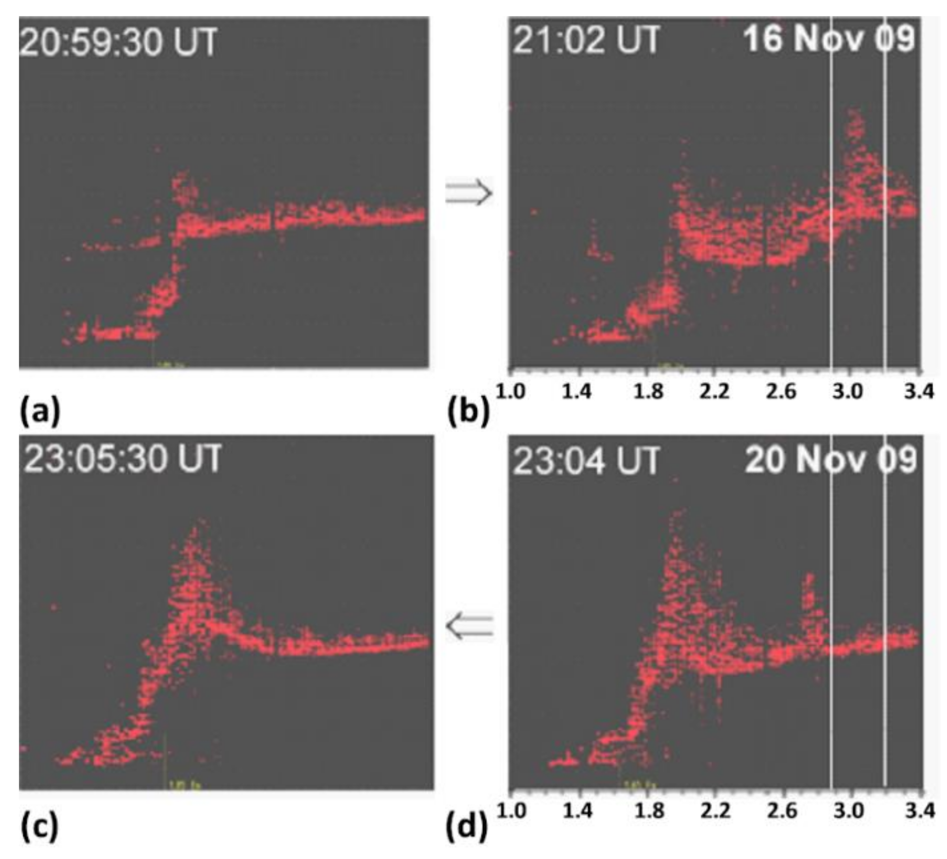
The impact of the natural cusp at foE on the competition between Langmuir PDI and upper hybrid PDI is further evidenced by the ionograms presented in Figure 3. The ionograms in Figure 3a,b were acquired on 16 November 2009 at 30 s before the heating experiment started and at the beginning of the moment when the O mode heater turned off after on for 2 min, respectively. As shown, the heating induced considerable virtual height spread as well as a bump located slightly below the HF reflection height. The ionograms in Figure 3c,d were acquired, on 20 November 2009, at 90 s after the heating experiment ended and at the beginning of the moment when the O mode heater turned off after on for 2 min, respectively. As shown, the heating also induced considerable virtual height spread as well as a bump but located slightly below the upper hybrid resonance layer. Ionograms in Figure 3a,c represent the background conditions in the two heating periods (21:00 to 21:02) on 16 November and (23:02 to 23:04) on 20 November. The natural cusp on 20 November was considerably large.
The ionograms in Figure 3 indicate that the natural cusp was small on 16 November, thus, Langmuir PDI prevailed. On the other hand, on 20 November when the natural cusp was large, Langmuir PDI was suppressed and upper hybrid PDI prevailed. Because the density cusp introduces anomalous loss of the HF heater, the upper hybrid PDI was not as strongly excited as the Langmuir PDI excited on 16 November. Consequently, the upper hybrid bump in Figure 3d is much smaller than the Langmuir bump in Figure 3b.
Monostatic UHF radar only detect backscattered lines, such as HFPLs and HFILs; on the other hand, parametric instabilities excite plasma waves with broad spectra, and their evolution to the nonlinear states cannot be revealed by the UHF radar. Moreover, due to the field-aligned nature of the upper hybrid waves, these waves also cannot be detected directly by the UHF radar. The distinctive virtual height bumps in Figure 2 and Figure 3 suggest that the digisonde can be a key diagnostic instrument to explore the nonlinear evolution of Langmuir waves and upper hybrid waves excited in the HF heating experiment.
2.3. Airglow Enhancement
Superthermal electron flux excites atomic oxygen via collision to produce airglow, which is emissions mainly at 630 nm and 557.7 nm. The minimum electron energies to stimulate airglow at 630 nm and 557.7 nm are 3.1 eV and 5.4 eV, respectively. Airglow enhancements were observed in the O-mode HF heating experiments. Electron plasma waves excited by parametric instabilities accelerate electrons through Doppler-shifted resonance interaction (quasi-linear diffusion) to reach the energy thresholds [6] for stimulating those airglows.
The enhancement of airglow at 777.4 nm was also observed as the O-mode HF heating wave was transmitted near the second and third harmonic of the electron gyro frequency [19,20]. The minimum electron energy to excite 777.4 nm emissions is 10.7 eV [19], which well exceeds the super thermal energy range and the capacity of quasi-linear diffusion.
Harmonic cyclotron resonances with electrons require the aid of finite Larmour radius effect [21], which is proportional to , where and , and are the transverse wavenumber and electron speed, and the electron gyrofrequency. The finite Larmour radius effect works to shift down the wave frequency to the fundamental cyclotron resonance frequency for Doppler-shifted cyclotron resonance interaction, as well as to provide a positive feedback to the interaction.
Thus, heating at the harmonic cyclotron resonances directly by the HF heating wave is not effective because the wavenumber of the HF heating wave is small. On the other hand, an O-mode HF heating wave can excite parametric instabilities (upper-hybrid OTSI and PDI) in and below the upper hybrid resonance layer to produce short scale upper hybrid waves, which can interact effectively with electrons at cyclotron harmonic resonance. In Section 5, the theory of harmonic cyclotron resonance interaction procedure will be elaborated, and numerical results will be presented to show the generation of very-high-energy electrons by the upper hybrid waves [22,23].
2.4. Energetic Electron Flux
In the O-mode HF heating experiments, electron fluxes in the energy range from 10 to 25 eV were detected in situ by a probe in rocket [24] as well as on the ground by UHF radar inferred by an ultra-upshifted frequency band [25] and by the CCD camera inferred by the airglow enhancement at 777.4 nm [19].
As described in Section 2.1, the spectral lines in the radar returns have a fixed wavelength equal to half of the radar wavelength; thus, an ultra-upshifted frequency band signifies that the radar scatterers are moving at ultra-high phase speeds. These high-speed electron waves, which are not plasma modes, are virtually formed by the wakefields of ultra-high energy electron bunches.
Plasma waves excited by the parametric instabilities are likely to be responsible for the electron acceleration to such a high energy level. Langmuir waves implement quasi-linear diffusion through a Doppler-shifted resonance interaction to produce super-thermal electrons. Upper hybrid waves further accelerate super-thermal electrons to ultra-energy level via Doppler-shifted harmonic cyclotron resonance interaction, which will be demonstrated by the numerical simulations of Section 5.
2.5. Artificial Ionization Layers (AILs)
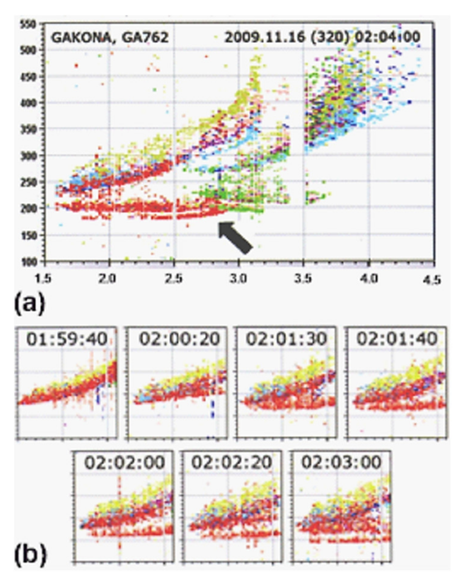
Optical emissions observed by Pedersen et al. [26,27] indicated that new ionization layers were produced by the O-mode HF heating wave at frequency (~2.85 MHz) set near double the electron gyro frequency. Digisonde [18] echoes, shown in Figure 4a, provided evidence to support the generation of artificial ionization layers, indicated by an arrow. The generation and development of AILs during the heating experiment are seen by a sequence of seven ionograms recorded from 01:59:40 to 02:03:00, as presented in Figure 4b. Ionization energy of the atomic oxygen “O” is 13.6 eV. Experiments [28,29,30] were further conducted during twilight and early evening hours in Alaska local time, when the photoionization was weak. The wave–ionosphere interaction occurs in the region around 230 to 250 km, where the O+ ions are dominant.
Experimental results show that the enhanced optical emissions (inferring ionization enhancement) descend in the background F-region ionosphere [31] and relatively thin artificial ionization structures, seen directly in the ionograms of the digisonde, are emerging from the lower F-region ionosphere and descending (Figure 4b) to settle at the base of the F-region (Figure 4a).
In later experiments with the heating wave frequencies set at 4.34 MHz and at 5.8 MHz, which are around the third and fourth harmonic of the electron gyro frequency, digisonde ionograms show that AILs also emerge from the base of the ambient F region as relatively thin layers, like those formed with the heating wave frequency set near the second harmonic of the electron gyro frequency. Experiments found that AILs were preferred to be generated with the heating wave frequency tuned either slightly above a harmonic of the electron gyro frequency or far below the second harmonic gyro frequency.
The power transfer from wave to the electron moving along the magnetic field, i.e., P∥ = −e Ezvez, depends on the phase of Ez which varies with time due to the mismatch frequency Δω ≠ 0. Although the phase is distributed randomly from 0 to 2π, there are electrons of appropriate phases that will gain energy from the wave, i.e., P∥ > 0 and vez increases. In the case of Δω > 0, Δω decreases to give a positive feedback to enhance wave–electron interaction. When Δω drops to a negative value, the feedback of the interaction becomes negative; thus, a sufficient large Δω0 is necessary to give adequate positive feedback interaction period for the generation of energetic electrons. On the other hand, if Δω0 is too large, the initial interaction will be too weak, and the available interaction spatial length will be too short to generate energetic electrons. When the heating wave frequency is far below the second harmonic of the electron gyro frequency, the excited Langmuir waves can resonantly interact with electrons through Doppler-shifted cyclotron resonance; at fundamental cyclotron resonance, the interaction does not need the aid of the finite Larmour radius effect, and positive feedback to the interaction can still be sufficient at large frequency mismatch.
The numerical results to be presented in Section 5 show that the parametrically excited upper hybrid waves can energize electrons to exceed 13.6 eV, the ionization energy of the atomic oxygen “O”, through the harmonic cyclotron resonance interaction [22,23]. Moreover, the parametrically excited upper hybrid waves have a frequency band, which it makes accessible for the match of cyclotron harmonic resonance over an altitude region. Thus, electrons, while moving downward, can be accelerated continuously along a slightly increasing geomagnetic field, through the Doppler-shifted harmonic cyclotron resonance interaction with a band of spatially distributed upper hybrid waves. It results in a major ionization occurrence at the bottom of the F region. This explains the descending feature of the enhanced optical emissions in the evolution of AILs and the emergence of AILs as relatively thin artificial ionization structures at the bottom of the F region.
2.6. Artificial Spread-F
Digisonde is HF radar, which probes the electron density distribution in the bottom side of the ionosphere. O-mode and X-mode sounding pulses with carrier frequency swept from 1 to 10 MHz are transmitted for sounding echoes, which are then recorded in an ionogram. An O-mode or a X-mode sounding echo represents the backscatter of a corresponding sounding pulse from a layer of the ionosphere, where the electron plasma density of the layer matches the O-mode cutoff density cm−3 or X-mode cutoff density cm−3 set by the carrier frequency f of the respective sounding pulse, where h and are the virtual height of the layer and the electron gyrofrequency. The virtual height h is determined by the time delay τ of the echo to be h = cτ/2, where c is the speed of light in free space. At HAARP site, can be converted to a true height profile by a profile conversion (NHPC) algorithm [32], which is available in the software program SAO Explorer [33].
The digisonde radiates at a large cone angle, each sounding pulse can be decomposed into many rays, which have different ray trajectories, and only backscattered rays can return to the digisonde and are recorded as the ionogram echoes.
In the unperturbed ionosphere, only a few rays, which are close to the vertical transmission, are backscattered. The virtual height traces of the sounding echoes in the ionogram have narrow virtual height spreads. When the ionosphere is perturbed, it also affects ray trajectories. In the presence of large-scale field-aligned density irregularities (FAIs with scale lengths of a few hundreds of meters to kilometers), ray trajectories [34] can be significantly modified as elaborated in Section 3.
In general, multiple incident rays (at different oblique angles) are backscattered to the digisonde receiver to produce multiple sounding echoes at the same radar frequency but at different return times [35], resulting in the spread of the virtual height traces. In the naturally perturbed ionosphere, the spread usually appears in the frequency band corresponding to the F region of the ionosphere and is thus termed “Spread-F”.
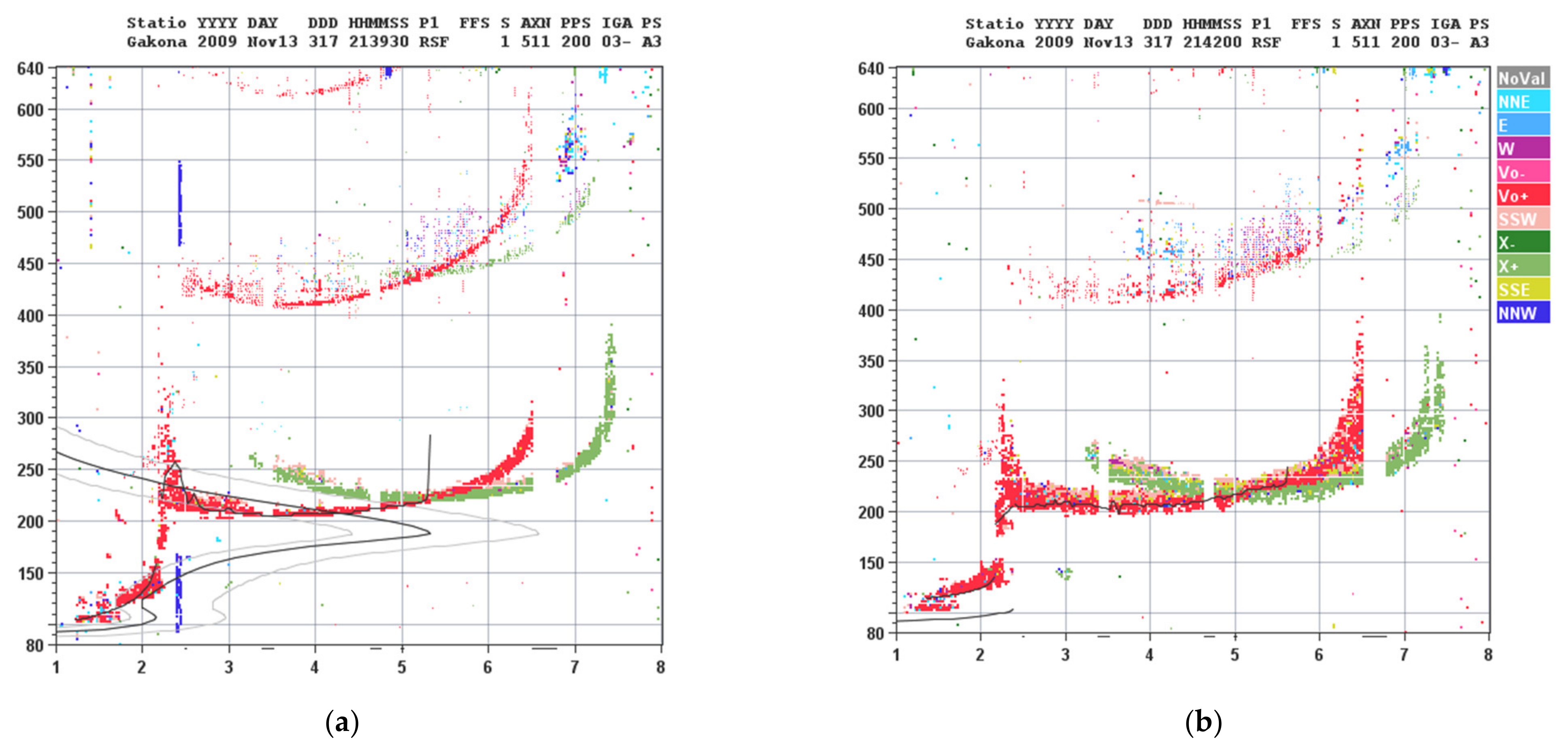
In HF heating experiments conducted on November 13, 2009 from 21:00 to 23:00 UTC (12:00 to 14:00 local time), spread-F induced by the O-mode HF heater at 5.75 MHz (slightly above the fourth harmonic of the electron gyrofrequency) has also been observed and is termed “artificial spread-F”. This is demonstrated in Figure 5 comparing a pair of ionograms without (Figure 5a) and with heating effect (Figure 5b) [34]. As shown, the artificial spread-F extends from 2.4 MHz (foF1 ~ 2.38 MHz) to foF2 ~ 6.4 MHz; on the other hand, the parametric instabilities excited by the O-mode heating wave of 5.75 MHz occur only locally near the HF reflection height (at 5.75 MHz) and around upper hybrid resonance region (at 5.57 MHz). Although the large-scale FAIs could be generated through the filamentation of the HF heating wave [36], the FAIs responsible for the virtual height spread appearing in Figure 5b are likely generated by the thermal instability [37] driven by the downward and upward heat flow from the heat sources (converted from the plasma waves excited by the parametric instabilities) located near the HF reflection region and near the upper hybrid resonance region.
2.7. Ionization Enhancement
In the 20 November 2009 experiment, although the O-mode heating wave frequency of 3.2 MHz was not close to an electron harmonic cyclotron resonance frequency, artificial ionization enhancement was observed together with artificial spread-F [34]. Experiments were conducted around local solar noon when the photoionization was strong and the wave-electron interaction occurred in the lower F region (<180 km) of the ionosphere, where the electron-ion effective recombination coefficient depends strongly on the electron temperature Te [38]. Anomalous electron heating through parametric instabilities and thermal diffusion it reduces the recombination coefficient to change the balance between the photoionization and the recombination loss over a large region. As a result, there is an electron density enhancement in the heated region below ~180 km.
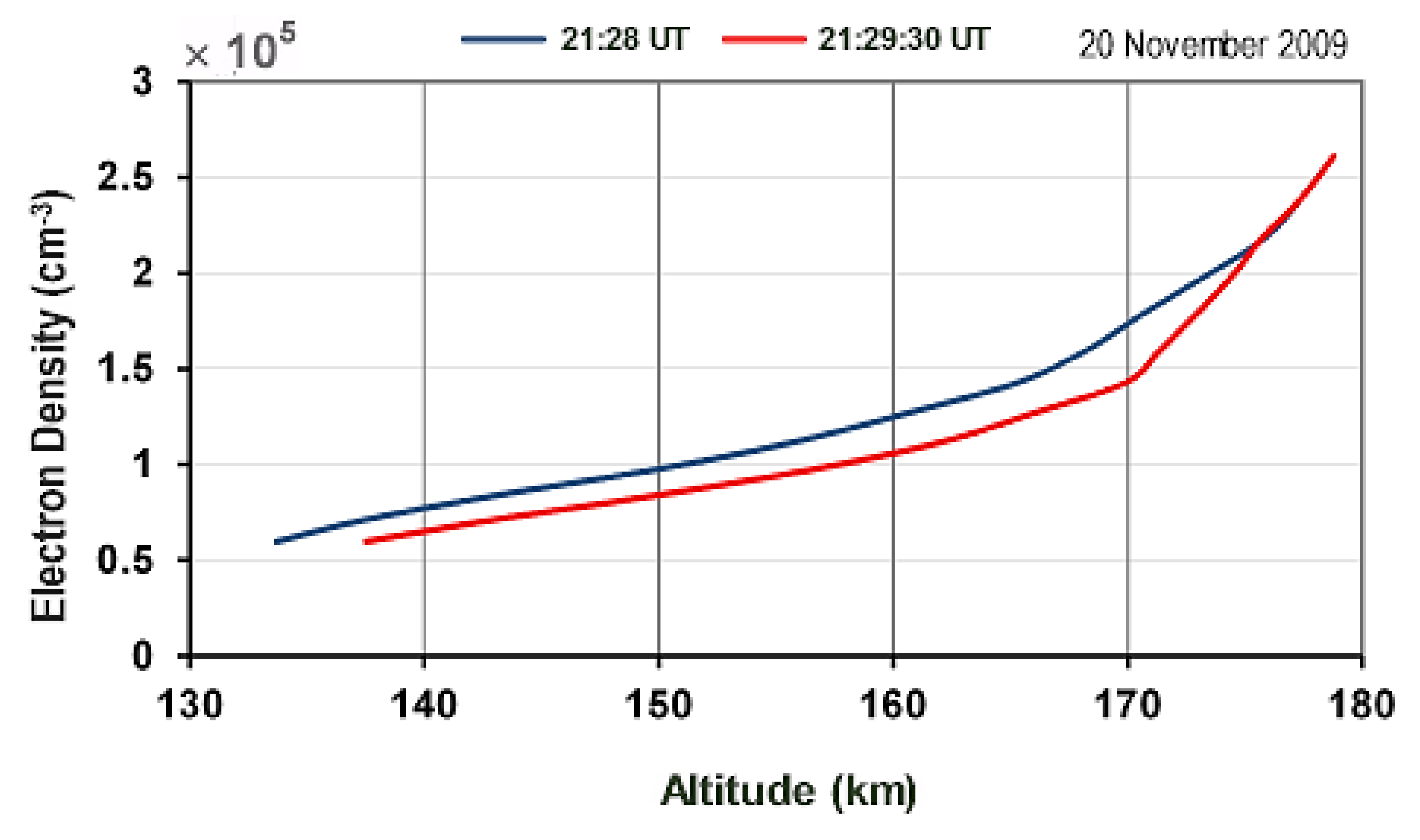
This is demonstrated in Figure 6, in which electron density distributions at times (a) 21:29:30UT, after the O-mode heater off more than 90 s and (b) 21:28:00UT, off within 10 s, are presented for comparison. As shown, the distribution at time (b) (i.e., blue curve) has a higher density in the entire modified region than that at time (a) (i.e., red curve). The percentage of the electron density increase exceeds 10% over a region extended in height (> 30 Km) from below to above the HF reflection height.
2.8. Artificial Cusp
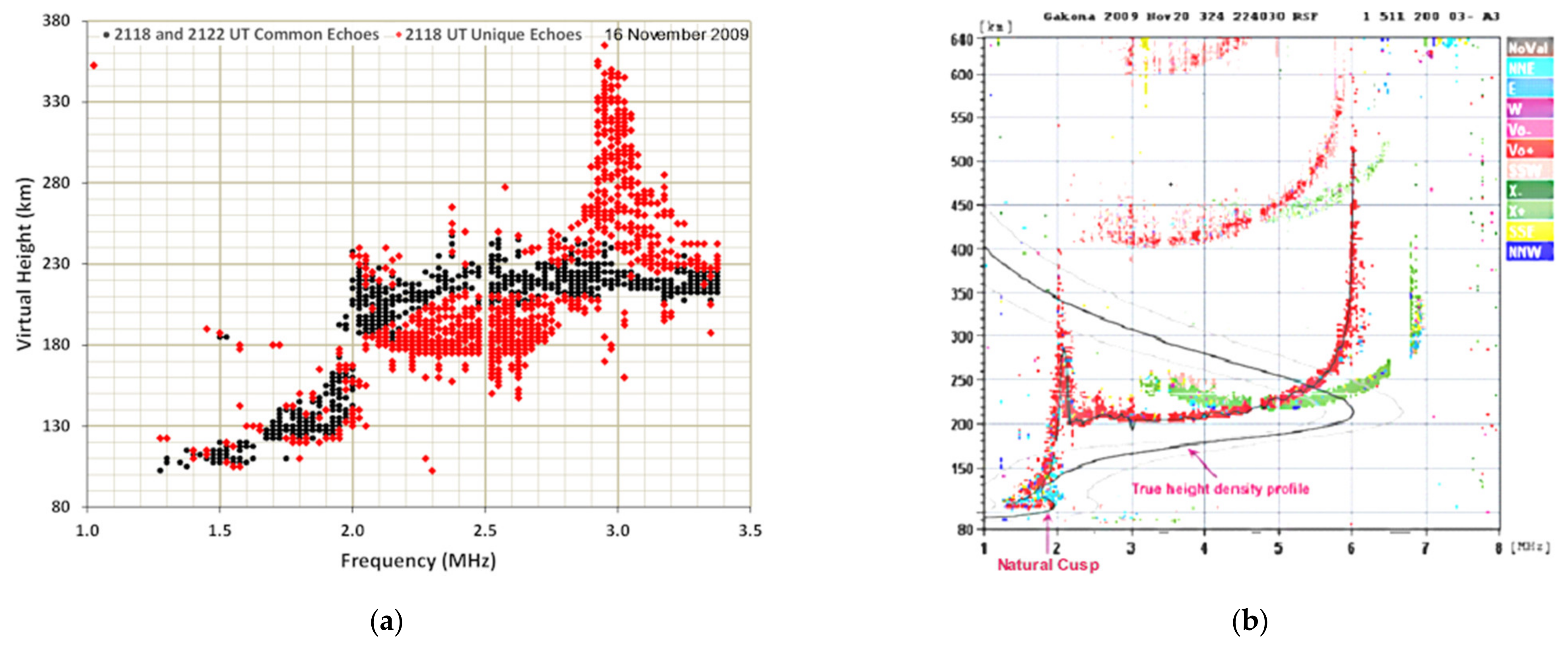
A virtual height bump usually occurs at frequencies near foE in the presence of an F1 layer, as shown in Figure 5a; the true height profile (the solid line plot) indicates that there is a density ledge (cusp) at foE, which retards the propagation of sounding signals with frequencies f close to foE, causing spread of the sounding echoes in virtual height in the form of a distinct bump. Spread-F normally extends over a frequency band in the ionogram and is recognized to be caused by the large-scale FAIs in the plasma. However, localized anomalous echo spread appearing as a bump in the ionogram trace has also been observed in the O-mode HF heating experiments conducted on 16 November 2009. This is exemplified in Figure 7a, showing a combined ionogram from a pair of heater-off ionograms acquired at 21:18 UT and 21:22 UT after the O mode heater of 3.2 MHz turned on at 21:16 UT for 2 min [12] and the X-mode heater of 3.2 MHz turned on at 21:20 UT for 2 min [12].
The ionogram in 21:18 UT shows considerable spread of echoes and contain a noticeable bump located at 2.92 MHz, slightly above the plasma frequency (fp = (f02 − fce2)1/2 ~ 2.88 MHz) of the upper hybrid resonance layer of the O-mode heating wave at f0 = 3.2 MHz, where fce ~ 1.4 MHz is the electron cyclotron frequency. This heating-induced bump in the ionogram trace is similar in its appearance to the natural virtual height bump induced by the density cusp at E-F1 transition layer (at foE ~ 1.96 MHz in the presence of an F1 layer as shown in Figure 7b); the similarity suggests that a heater-stimulated ionization ledge (cusp) appears near the upper hybrid resonance layer, which causes the virtual height spread in the form of a bump peaked slightly above the upper hybrid resonance layer [12]. This ledge can be created by the thermal pressure force arising from the Langmuir waves (i.e., the localized Langmuir waves form a caviton), which are excited parametrically by the HF heating wave. The matching height of the Langmuir wave drops due to the increase of the effective electron temperature, which is proportional to the total spectral intensity of the Langmuir waves.
The experiment was conducted around local solar noon when the photoionization was strong and the wave–electron interaction occurred in the lower F region (<180 km of the true height) of the ionosphere, where the electron-ion effective recombination coefficient depends strongly on the electron temperature Te [38]. The heat diffusion from the Langmuir PDI region downward and upward excites thermal instability to generate large-scale FAIs [37] as well as to cause ionization enhancement over a large region. An ionization enhancement, like that presented in Figure 6, was observed. On the other hand, the combined ionogram presented in Figure 7a shows that the heating wave induces a downward spread of the ionogram trace in the region from 2.1 to 2.8 MHz, different from that shown in Figure 5b in which the enhanced Spread-F appears with an upward-spread of the virtual height in the ionogram trace. It is likely the spread in Figure 7a is caused by a different mechanism; the down-going Langmuir waves evolve into nonlinear periodic plasma waves propagating along the magnetic field, which backscatter incoherently the sounding pulses to give rise to downward spread of the ionogram trace.
In sum, these observed phenomena are ascribed to various linear and nonlinear wave–plasma and wave–wave interactions instigated by the Langmuir waves, upper hybrid waves, and density irregularities, generated by the HF heating waves. Theoretical formulation and analysis of parametric instabilities and instigated interaction processes are presented in Section 4 as the theoretical basis of HF heating induced phenomena.
3. Ray Tracing
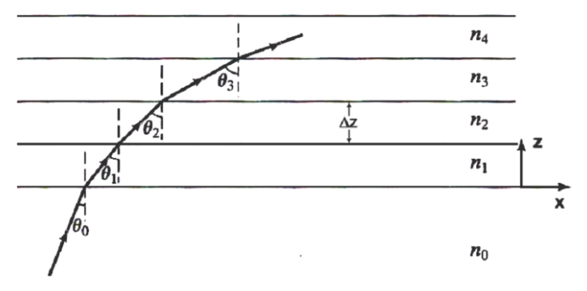
One approach to characterize wave propagation in the ionosphere is “ray tracing”. It is applicable when the wave front extends uniformly over several wavelengths and the inhomogeneity scale lengths of the medium are large in comparison to the wavelength, and particularly, the wave has a dominant frequency. In this situation, the wave may be treated as a ray and its trajectory is tracked to explore wave propagation and the ionospheric plasma. The ionosphere is stratified into layers and the Snell’s law of refraction is applied at the interface of two adjacent layers to setup the ray trajectory equation. This is illustrated by applying the arrangement shown in Figure 8, in which an inhomogeneous medium with refractive index n(z) is approximated by a series of plane slabs of thickness Δz, where Δz → 0 and each slab i has a uniform refractive index .
As shown in Figure 8, a ray is incident from a uniform medium (e.g., below the ionospheric plasma) of refractive index at an angle, , with respect to the vertical axis into this inhomogeneous medium; the Snell’s law is applied at the interface of two adjacent slabs j and j+1 to determine the moving direction of the ray; < < … is assumed in the plot (however, in the case of propagating upward into the ionospheric plasma, it is > > ….).
The path of the ray in each slab is a straight line, and one can identify the relations: and , where is the horizontal displacement of the ray after transit through slab i. In the limit of Δz → 0, these two relations become and , and a trajectory equation is derived to be
If n2 can be modelled by a second-order polynomial, i.e., n2(z) = a + bz + cz2, (1) can be integrated analytically; otherwise, it is integrated numerically.
3.1. General Formulation of Ray Trajectory Equations
Consider a general case that wave propagation is governed by a dispersion equation with the generic form [39]
G(k, ω; r, t) = 0.
We now introduce a generic variable “τ” and take a total τ derivative on (2), it yields
The four terms in (3) are arranged into two groups to be
where the first group of terms is related to the time variation of the media, while the second group related to the spatial variation of the media. Because (4) is obtained from a general approach and the spatial variation and temporal variation are separable, its general solution requires that the following two relations be satisfied simultaneously:
and
where and because r and k and t and ω are independent to each other; thus (5) and (6) deduce to the following relations
In principle, (2) can be solved to obtain, for instance, ω = ω(k; r, t); in other words, there are only three independent variables in (2). Choose r, t, and k to be independent variables and ω a dependent variable, i.e., G(k, ω; r, t) = G(k, r, t; ω(k, r, t)) then take partial derivatives of (2) with respective to the three independent variables k, r, and t, respectively, it obtains the following three relationships
With the aid of (8a) and (7d), (7a) becomes
which leads to
With the aid of (8b) and (7d), (7b) becomes
which leads to
With the aid of (8c) and (7d), (7c) becomes
Equations (9) to (11), subject to a set of initial conditions, determine the ray trajectory in the phase space (i.e., r–k space). In essence, these are the Hamilton’s equations of motion with ω and k to be the Hamiltonian and momentum of the ray.
3.2. Ray Trajectories of Sounding Pulses-Spread-F
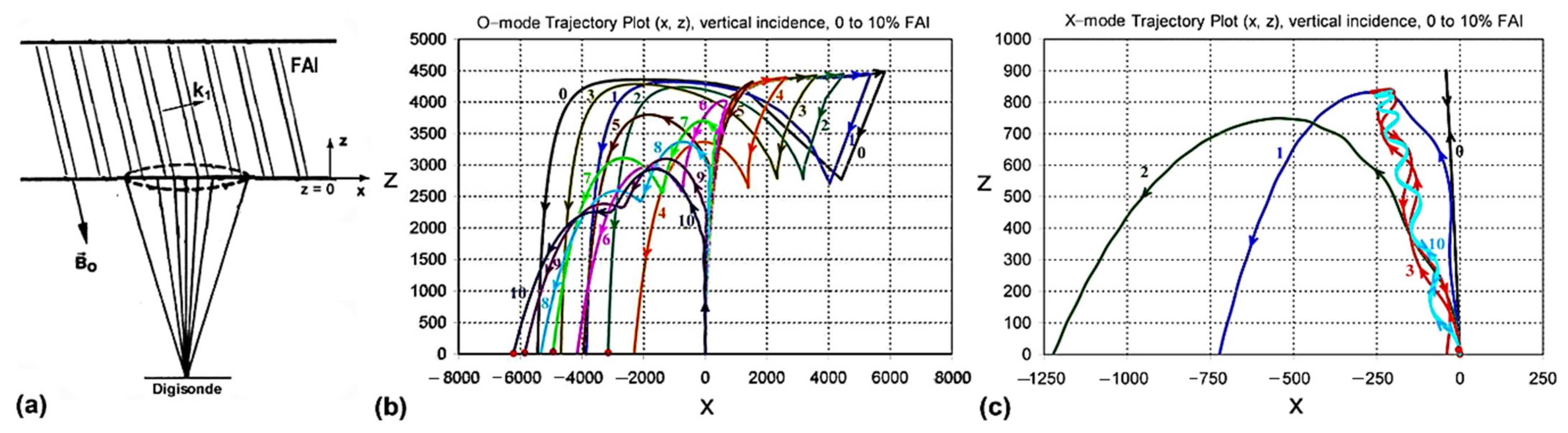
This ray tracing technique is applied to explain the virtual height spread (e.g., Figure 5b) of the ionogram trace observed in the HF heating experiments. Digisonde (ionosonde), an HF radar, is a remote-sensing device for monitoring the plasma density profile of the bottom-side ionosphere. It transmits sounding pulses upward and records the return echoes in an ionogram as the virtual height trace. Digisonde radiates at a large cone angle, each sounding pulse can be decomposed into many rays, which have different ray trajectories, and only backscattered rays can return to the digisonde and are recorded as the ionogram echoes. In the unperturbed ionosphere, only a few rays, which are close to the vertical transmission, are backscattered. Thus, the virtual height traces of the sounding echoes in the ionogram have narrow virtual height spreads. However, when the ionosphere is perturbed in the presence of large-scale field-aligned density irregularities, ray trajectories can be significantly modified as elaborated in the following.
A carton of large-scale FAIs appearing in the F region of the ionosphere is presented in Figure 9a; x and z axes are in the horizontal and vertical directions. A sounding pulse of the digisonde is decomposed into a bunch of rays as also shown in Figure 9a. Only plasma affects ray trajectory, thus, from the ground to the reference layer, z = 0, rays are assumed to propagate in a free space, where the plasma density is still low and FAIs do not extend to. Ray trajectories from z = 0 up to their reflection layers and returning to z = 0 are determined via ray tracing technique. In this region, the background plasma has a density distribution , where and L are the plasma density at the reference layer, z = 0, and the inhomogeneity scale length of the background plasma, respectively. FAIs are represented by a single sinusoidal function with a spatial period d and an amplitude ΔN, i.e., , where and is the magnetic dip angle; at Arecibo, HAARP, and EISCAT, respectively.
In the model, plasma is uniform in the y direction, only two-dimensional trajectories on the x-z plane are considered in the numerical analysis; (9) and (10) become
and
Because the ionospheric plasma and FAIs can be stationary in the propagation period of a ray, , (11) leads to ; thus is a constant of motion. With the aid of the dispersion relation , right-hand side terms of the Equations in (12) and (13) can be expressed explicitly.
Digisonde transmits linearly polarized sounding pulses, which can be decomposed to RH- and LH-polarizations representing O-mode and X-mode sounding pulses. The dispersion equations for obliquely propagating O-mode and X-mode heating waves are given approximately by
and
where the parallel and perpendicular (to the magnetic field) components, and of the wavevector are related to the x and z components, and of the wavevector by and ; and With the aid of (14) and (15), right hand side terms of the equations in (12) and (13) can be expressed explicitly for the O-mode and X-mode sounding rays, respectively.
In the numerical calculation, FAIs are represented by a single sinusoidal function with a spatial period of 200 m and an amplitude ΔN; the background plasma density has a linear scale length L = 30 km. Figure 9b demonstrates the change of the trajectory of a vertically incident O-mode ray of 2.8 MHz in the presence of FAIs with the amplitude ΔN increased from 0 to 0.1 N0, where N0 is the plasma density at a reference layer, z = 0, having a plasma frequency (i.e., 3.2/√2 MHz). In the absence of FAIs (ΔN = 0), the vertically incident ray is backscattered. However, in the presence of FAIs (ΔN/N0 = 0.01 to 0.1), the vertically incident ray is not backscattered anymore.
A similar demonstration for the vertically incident x-mode ray of 2.8 MHz is presented in Figure 9c. As shown, the vertically incident ray is backscattered also only in the absence of FAIs (ΔN = 0). In fact, the vertically incident ray is ducted by the FAIs (for , the return signal propagates along the geomagnetic field, rather than propagating vertically downward. The x and z axes in Figure 9b,c are normalized to k0 = ω0/c, where is the frequency of the sounding pulse. For example, at 2.8 MHz, ; thus, the (x, z) axes for 2.8 MHz ray are normalized to 17.05232 m. The normalization is inversely proportional to the frequency, thereby it decreases to 13.64 m for 3.5 MHz ray.
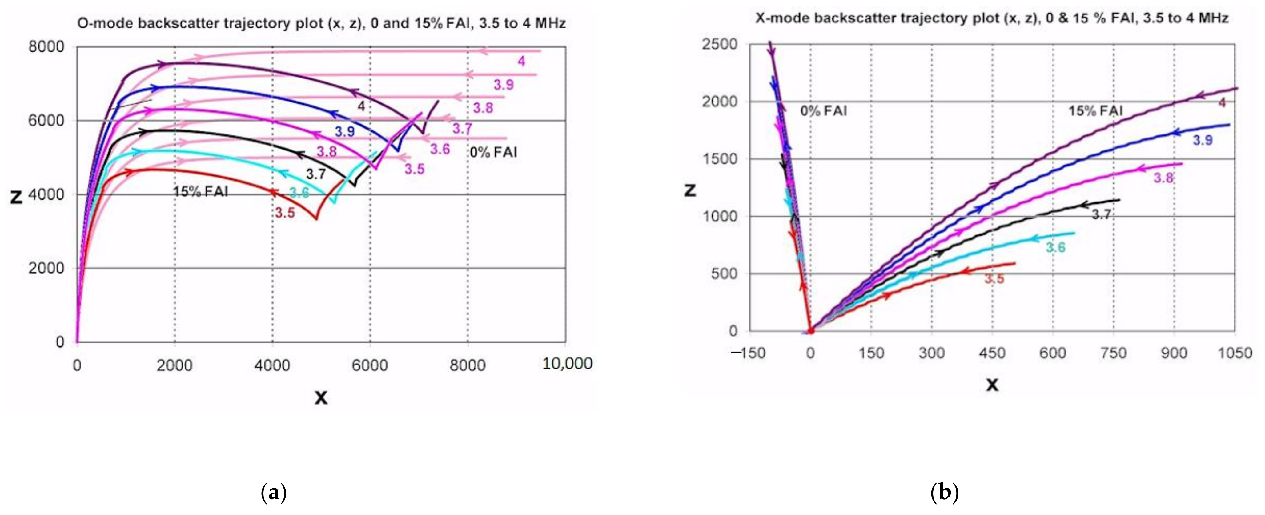
Therefore, in the presence of FAIs, the traces in an ionogram are not contributed by the returns of the vertically incident rays. In order to achieve backscatter, the incident direction of the ray at the reference layer, z = 0, must have an off vertical angle. The trajectories of backscatter rays in the presence of 15% FAIs for both O- and X-mode sounding signals from 3.5 to 4 MHz are determined. 15% FAIs are relatively large for the general situation; it is adopted in the simulations for a better contrast. The results are shown in Figure 10, the backscatter trajectories in the absence of FAIs are also plotted for comparison.
As shown in Figure 10a, the trajectories of the O-mode backscatter rays [3.5 (red), 3.6 (green), 3.7 (black), 3.8 (pink), 3.9 (blue), 4 (brown) MHz] are modified significantly by the FAI from those (light pink) in the absence of FAI, however the incident off-vertical angles are very small (); on the other hand, as shown in Figure 10b, the off-vertical angles of the x-mode backscatter rays in the presence of FAI are very large, and this off-vertical angle () increases as the frequency of the sounding signal decreases. The off-vertical angle also increases with the increase of the FAI amplitude. In general, multiple incident rays (at different oblique angles) are backscattered to the digisonde receiver to produce multiple sounding echoes at the same radar frequency but at different return times [35], resulting in the spread of the virtual height traces. In the HF heating experiments, large-scale FAIs are generated by the O-mode heating waves, causing a spread of the virtual height traces like the natural Spread-F; the heating-wave-induced Spread-F is termed “Artificial Spread-F”.
4. Parametric Instabilities Excited in HF Heating Experiments
Plasma supports high-frequency and low-frequency modes; in the absence of external sources, these modes present in plasma as thermal fluctuations. A large-amplitude, high-frequency wave, , (either electromagnetic (EM) or electrostatic (ES)), can be a pump wave, which excites high- and low-frequency plasma waves concurrently [39]. The electric field of the high frequency pump wave sets up a quiver motion in the electron plasma at velocity . On the other hand, electrons and ions oscillate together to maintain quasi-neutrality, i.e., , in the low frequency plasma wave field; it facilitates the low-frequency plasma wave to buildup plasma density perturbation . A coupling of the pump wave and the low-frequency plasma wave induces a high-frequency space charge current density, , in the electron plasma. Such a current drives beat waves, , with the wavevectors and frequencies satisfying the matching conditions:
These beat waves, in turn, also couple with the pump wave to induce in the electron plasma a low-frequency nonlinear force, which has the same frequency and wavevector as the density perturbation, , to drive this density perturbation. When the couplings generate large enough positive feedback to overcome linear losses of the coupled waves, instability is excited to grow the coupled plasma waves exponentially in the expense of the pump wave energy. This is called “parametric instability”; a pump wave, , decays to two sidebands, and , through coupling to a low-frequency decay mode, . Parametric coupling is imposed by the frequency and wavevector matching conditions; further, the instability requires the pump electric field intensity to exceed a threshold. When the decay mode, , has a finite oscillation frequency, two sidebands cannot satisfy the same dispersion relation concurrently. The frequency-upshifted sideband, , has large frequency discrepancy from the plasma mode and can be disregarded to simplify the parametric coupling to be three-wave interaction.
Parametric excitation of Langmuir/upper hybrid waves, , and low-frequency plasma waves, , by the electromagnetic or Langmuir/upper hybrid pump waves, , in the bottom-side of the ionosphere, are explored in the following, where , , and denote electric field of a pump wave, electrostatic potential of the Langmuir/upper hybrid sideband, and density perturbation of a low frequency decay mode, respectively. Langmuir waves can have large oblique propagation angles (with respect to the geomagnetic field ), upper hybrid waves have near 90° propagation angles, and low-frequency plasma waves include ion acoustic/lower hybrid waves as well as purely growing modes.
The most likely parametric instabilities excited directly by a HF heating wave in the bottom-side of the ionosphere include 1) oscillating two-stream instability (OTSI), and 2) parametric decay instability (PDI), in both mid-latitude and high-latitude ionosphere [4,40,41]. The sidebands are Langmuir waves and upper hybrid waves. The instabilities with Langmuir waves as sidebands must compete with those excited in the upper hybrid resonance region, where the upper hybrid waves are the sidebands of the instabilities. The wavenumber of the HF heating wave is much smaller than the wavenumbers of the electrostatic sidebands and decay modes, thus a dipole pump, i.e., , is generally assumed. As the excited Langmuir/upper hybrid sidebands grow to large amplitudes, they also become pump waves to excite parametric instabilities [42,43].
When the theory is used to explain the observations, it is noted that HFPLs and HFILs are monitored by UHF and VHF backscatter radars; those lines are associated with plasma waves propagating oblique to the geomagnetic field at an angle conjugate to the magnetic dip angle. Moreover, upper hybrid waves, lower hybrid waves, and field-aligned purely growing modes cannot be detected.
The coupled mode equation for the Langmuir/upper hybrid sideband is derived from the electron continuity and momentum equations, together with the Poisson’s equation, to be [44]
where 〈 〉 represents a filter, which only keeps terms with the same phase function as that of the function ϕ on the left-hand side; , , , and m, are the electron cyclotron frequency, plasma frequency, thermal speed, and mass, respectively. (16) is derived from the fluid equations, however the kinetic effect of electron Landau damping is included phenomenologically in the collision damping rate, i.e., , which is the effective electron collision frequency, where , a sum of the electron-neutral elastic collision frequency, , and the electron-ion Coulomb collision frequency, , here lnΛ ≅ 15 is assumed; is in cm−3, is in K, and is the electron plasma frequency], and , a phenomenological collision frequency to represent electron Landau damping.
The low-frequency wave fields move both electrons and ions, hence the formulation of the coupled mode equation for the low-frequency decay mode, , includes electron and ion fluid equations. Because electrons and ions move together in the low frequency field, the formulation is simplified by introducing quasi-neutral condition: . The ion fluid equations are similar to the electrons except that the electron mass m is changed to the ion mass M, the charge −e changed to e, and the collision terms in the electron and ion fluid equations are modeled differently by νei(ve − vi) + (νen + νeL) ve and , respectively, where , is the ion-neutral collision frequency, represents ion Landau damping on the low frequency decay mode, and .
Neglecting the electron inertial term and the ion convective term in the momentum equations, these two momentum equations are combined into a one fluid equation, where the relations are applied. This equation is then combined with the ion continuity equation to derive a coupled mode equation, for the low-frequency (ion acoustic/lower hybrid) decay mode [45]
where is the ion cyclotron frequency, the ion acoustic speed, and M the ion (O+) mass; is applied; , and . The coupling terms and = 〈〉 arise from plasma nonlinearities. The linear responses of the electron density and velocity to the total high frequency wave fields are used to present these coupling terms.
In the following, parametric decays of an O-mode EM dipole pump, , into Langmuir/upper hybrid sidebands, , and a low-frequency decay mode, , (a purely growing or an ion acoustic mode / FAI or a lower hybrid mode) in the spatial region below the HF reflection height are studied. and denote the sideband’s electrostatic potentials and the density perturbation of purely growing or ion acoustic/FAI or lower hybrid mode, respectively; and , i.e., and ; ; and are imposed by the frequency and wavevector matching conditions. The O-mode heating wave field is given to be
where , and c.c. represents complex conjugate. It is noted that varies with the location (i.e., altitude); for instance, in the upper hybrid resonance region, and thus , where, neglect D region loss, P is the radiated power of the HF heater, G is the heater antenna gain, and R is the distance between the HF antenna and the excited upper hybrid resonance region; usually, it expresses , and is called effective isotropic radiated power (EIRP). Near the HF reflection height, and thus .
With the aid of (18), Equations (16) and (17) become
and
where
Equations (19) and (20) are analyzed in the k-ω domain, where the spatial and temporal variation of physical functions in (19) and (20) are set to have the form of , where κ and are the appropriate wavevector and complex frequency of each physical quantity. Thus (19) and (20) are converted to the coupled algebraic equations to be
and
where ; (21) is simplified with the condition ; .
In the following, the coupled mode algebraic Equations (21) and (22) are employed to analyze parametric instabilities excited in the ionospheric HF heating experiments.
4.1. OTSI and PDI near the HF Reflection Height
The RH circularly polarized HF heating wave propagates to the region near the reflection height, and it converts to the O-mode with the electric field .
4.1.1. OTSI—Excitation of Langmuir Sidebands Together with Purely Growing Density Striations by the HF Heating Wave
The parallel (to the magnetic field) component of the wavevector of the small-scale purely growing mode is not negligibly small, and the density striations are mainly driven by the parallel component of the ponderomotive force induced by the high frequency wave fields. Apply the condition ~ >> to simplify (22) and set and , (21) and (22) are combined to be
where .
Set in (23), the threshold field is obtained to be
It shows that the threshold field of OTSI varies with the propagation angle θ and wavelength λ of the Langmuir sidebands as well as the location of excitation (i.e., Δω2). The threshold field (24) has the minimum
when the (k,θ) lines are excited in a preferential layer at altitude h(k,θ), where and
4.1.2. PDI—Decay of HF Heating Wave to Langmuir Sideband ϕ(ω, k) and Ion Acoustic Wave
The coupled mode equations (21) and (22) are combined to a dispersion equation
When the instability is excited at the matching height h of its Langmuir sideband (k, θ), i.e., and , the minimum threshold field is obtained to be
Equations (25) and (27) show that the layers of exciting OTSI and PDI move downward and the threshold fields increase as the oblique propagation angles θ of the OTSI and PDI lines increase. When the heating wave field is large, the Langmuir sidebands excited by the OTSI and PDI will have angular (θ) and spectral (k) spread lines, distributed in altitude layers, where are higher and narrower for the OTSI excitation layer than that for the PDI layer.
4.2. Upper Hybrid OTSI and PDI Excited near the Upper Hybrid Resonance Layer
4.2.1. OTSI—HF Heating Wave Decaying to Upper Hybrid Sidebands and Field-Aligned Density Irregularities
The O-mode HF heating wave can access the upper hybrid resonance layer, which is located below the O-mode HF reflection height. In high-latitude regions, such as at Tromso, Norway and Gakona, Alaska, RH circularly polarized heating wave can be transmitted along the geomagnetic field. In the region near the upper hybrid resonance layer, the heating wave field still remain at RH circular polarization, i.e., ; the heating wave decays to two upper hybrid sidebands and a field-aligned purely growing mode , where .
Equations (21) and (22) are analyzed in the same way to be combined into a dispersion equation for the upper hybrid OTSI to be
where .
With , where , the minimum threshold field is obtained to be
4.2.2. PDI—Decay of HF Heating Wave to an Upper Hybrid Sideband ϕ(ω, k) and a Lower Hybrid Decay Wave
A dispersion equation is derived, by combining (21) and (22), to be
where is assumed.
The minimum threshold field of the instability excited at the matching height of its upper hybrid sideband is obtained to be
where , , and . The plasma frequency at the matching height is ; in other words, the preference region of exciting upper hybrid PDI is below the upper hybrid resonance layer.
The definitions of the symbols in (25), (27), (29), and (31) are summarized in the following: The ion acoustic speed and the electron thermal speed ;are the HF heating wave, ion acoustic, lower hybrid, electron plasma, and electron and ion cyclotron radian frequencies; , is electron-neutral elastic collision frequency, is the electron-ion Coulomb collision frequency, , and is twice of the electron Landau damping rate; , and is twice of the electron Landau rate on lower hybrid wave; , is the ion-neutral collision frequency, is twice of the ion Landau damping rate on ion acoustic wave; ξ = 1 + (M/m)(/); θ is the oblique angle of the wavevector with respect to the geomagnetic field; accounts for frequency mismatch, where .
4.3. Height Separations of the Instability Layers in the Bottom-Side of the Ionosphere
Let be the HF reflection height, Langmuir PDI height, and upper hybrid resonance layer height, and the corresponding electron plasma frequency at each height, respectively. In the small region from the upper-hybrid resonance layer to the HF reflection layer, a linear increasing plasma density profile is assumed, where is the electron density at (i.e., ), L is the linear scale length, and Δh is the distance below (i.e., ). With the aids of the HFPL dispersion relation and the definition of the upper-hybrid resonance frequency, this leads to ; then, are derived to be
and
where is the wavenumber of the UHF radar.
The following parameters corresponding to the HAARP site are adopted: m/s, , Rad/s, and MHz. Then (32) and (33) give ~ 0.0258L and ~ 0.114L ~ 4.4, leading to km for L ~ 34 km.
4.4. Impact of Double Resonances on Parametric Excitation of Upper Hybrid PDI
Double resonances is the situation where the upper-hybrid sideband of the upper-hybrid PDI excited in the upper hybrid resonance region is also in resonance with electrons at the Doppler-shifted nth harmonic cyclotron resonance, i.e., , where the upper-hybrid frequency . The frequency matching condition of the upper-hybrid PDI, can be satisfied if but close to . The lower-hybrid wave frequency at HAARP is given to be kHz, where . For ξ = 3, ~ 14.4 kHz.
A frequency sweep method can be applied to achieve a double resonance situation. It slowly sweeps the heating wave frequency from to a frequency covering the lower-hybrid wave frequency and the Doppler-shifted frequency Δf = . The linear velocity response of the electrons in the upper-hybrid wave field is given to be . At the Doppler-shifted cyclotron harmonic resonance, , there is an additional resonance response, ascribed to the finite Larmour radius effect; it is derived to be , where is the modified Bessel function of the first kind. The total electron velocity response to the upper-hybrid wave becomes ; the electron ponderomotive force, driving the lower-hybrid waves, is then enhanced by . It lowers the threshold field, given in (31), by a factor and elevates the growth rate by g2; thus, the upper-hybrid and lower-hybrid waves will be intensified as the finite Larmour radius factor is not too small. For 0.1, it requires that the wavelength of the upper-hybrid wave is less than 0.3 m, i.e., ≤ 0.3 m.
4.5. Instabilities under Double Resonance Situation
It was shown by Huang and Kuo [46] that when the heating wave frequency ω0 is near the third harmonic electron cyclotron resonance frequency, i.e., , upper-hybrid OTSI is suppressed by the parametric excitation of the electron Bernstein sidebands and small-scale FAIs. As a result, the source upper hybrid waves of the downshifted maximum (DM) lines of the stimulated electromagnetic emissions (SEEs) [47] is effectively suppressed; it explains the quenching of the DM feature in the SEE spectrum observed in the ionospheric heating experiments. However, the upper-hybrid PDI, which decays the HF pump wave into upper-hybrid sidebands and lower hybrid decay modes, can still be excited in the region below the upper-hybrid resonance region. As , upper-hybrid (OTSI and PDI) instabilities are excited in the upper-hybrid resonance region as well as in a large region underneath. In this case, upper-hybrid instabilities deplete the HF heating power considerably before the HF heating wave reaches the PDI layer, thus the Langmuir PDI is suppressed.
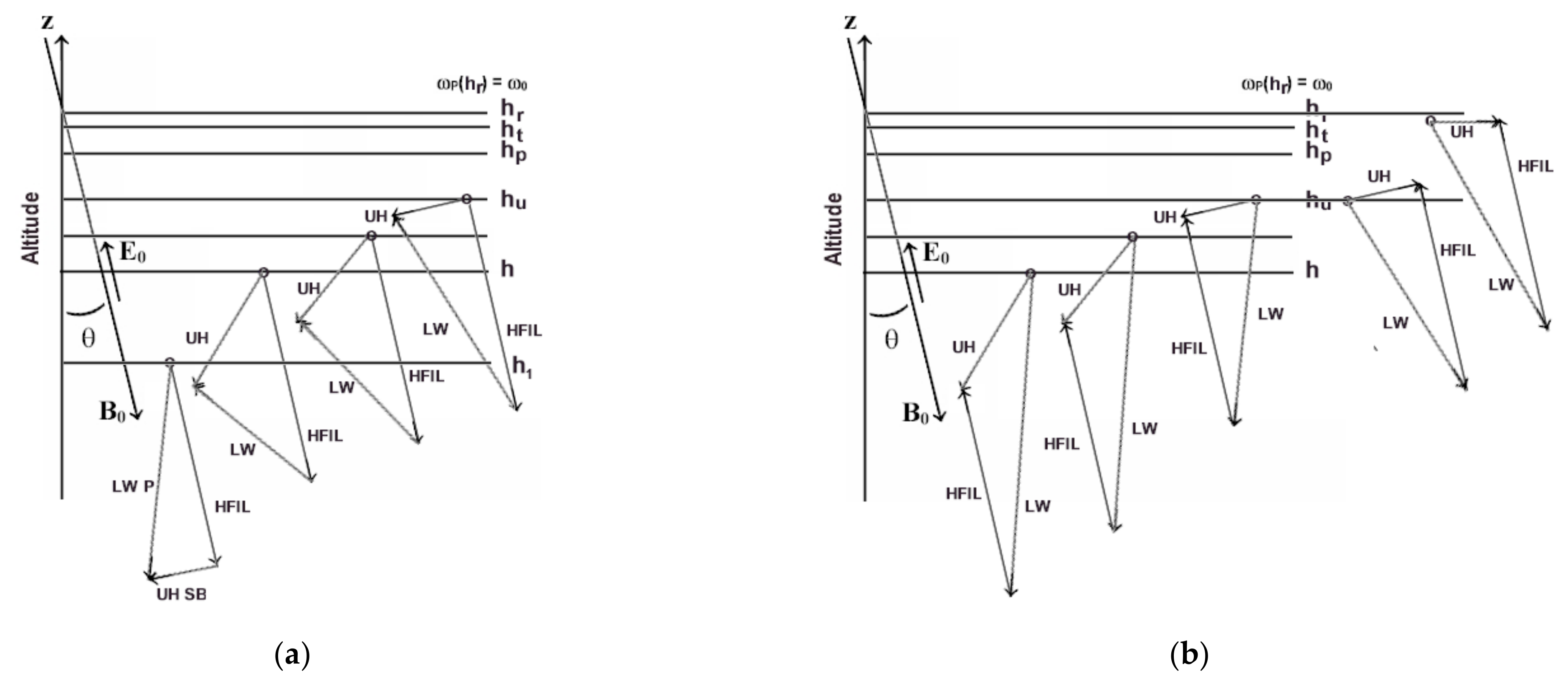
On the other hand, as the heating wave frequency ω0 is ramping-up swept to exceed nΩe (i.e., ), the frequency matching condition, , of the upper-hybrid PDI and the gyro-harmonic resonance condition , can be satisfied simultaneously in the same altitude region, where and = . Although double resonance suppresses upper-hybrid OTSI, it enhances the excitation of upper-hybrid PDI as discussed in Section 4.4; however, the upper-hybrid PDI zone is narrow; the instability will not be able to suppress the Langmuir PDI/OTSI. Langmuir PDI generated both up-going and down-going HFILs; but only the down-going HFILs will continuously propagate downward. On the other hand, the strongly excited upper-hybrid sidebands propagate downward and upward as electrostatic pump waves [48] that can cascade to down-going Langmuir sidebands and up-going ion-acoustic waves as well as up-going Langmuir sidebands and down-going ion-acoustic waves over an additional altitude range below . In terms of the wavevector matching conditions for the generation of up-going/down-going HFILs, the cascade processes are illustrated in Figure 11a,b, respectively [49]. Upward propagating upper-hybrid waves stop at a height near the HF reflection layer (at , as shown in Figure 11b).
The Langmuir sidebands in the two cascade instabilities have different wavenumbers and the oblique angles to the magnetic field. The cascade process involving up-going Langmuir sidebands (Figure 11b) has a higher threshold field (due to larger oblique angle) and lower growth rate (due to smaller wavenumber) than the other one involving down-going Langmuir sidebands (Figure 11a). Because the mode characteristic of the HFILs is not sensitive to the background plasma density variation, down-going HFILs mainly attribute to those generated via Langmuir PDI.
5. Harmonic Electron Cyclotron Resonance Interactions
The motion of an electron, starting at origin and interacting with the excited upper hybrid wave field, , in a uniform magnetic field , is considered, where and is an even function of k; thus, the initial wave field amplitude at origin is given by . The trajectory of the electron is governed by the equations: and , where is the electron cyclotron frequency. The trajectory equations are integrated to be
where , and ; ; and .
At Doppler-shifted cyclotron resonance, , the trajectory would be that determined by the resonant (secular) terms together with small perturbations oscillating at high frequencies due to the non-resonant interactions. is the harmonic cyclotron shifted wave phase velocity along the magnetic field and the resonant electrons propagate along the magnetic field in the same direction as that of the wave when .
In the present work, we will focus on the generation of energetic electrons, rather than the bulk heating, which is not directly relevant to the experimental observations. Hence, the non-resonant interaction terms in the trajectory functions (34) to (36) are neglected to focus only on the resonant trajectory. The x coordinate of the electron is obtained to be [21]
where and α and β are determined self-consistently to be
where is the Bessel function of order m, , and ; , , and .
Substituting (37) into (35) and (36) yields
With the aid of (38), (39), and (41), the temporal evolution of the electron temperature and electron distribution function can be determined. In the collisionless limit, the evolution of the distribution function follows the equation along the trajectories governed by (37) and (40) to (42). This equation provides the relation , subjected to the fact that are related to through (37) and (40) to (42). Therefore, for a given initial distribution , (e.g., a Maxwellian ), the time evolved distribution function under the resonance heating limit may be determined. The kinetic perpendicular temperature is then given by .
In the following formulation of harmonic cyclotron resonance interaction between electrons and upper hybrid waves [23], the approximation is applied, the new notations F = α and , are introduced, and the relations and are employed.
5.1. Second Harmonic Cyclotron Resonance Case (n = 2)
We keep only the term in (38) to (42) and for ; (38) and (39) are converted to the differential equations
where and . After the spectral integration, we obtain and , where ; the even function property of is applied and is close to the wavenumber of the spatial spectral peak of the upper hybrid wave. The value of depends on the initial velocity (speed and phase angle) of the electron and the field intensity. The difference between the parallel velocities causes detuning on the resonance, which results in the reduction of the acceleration. We consider the optimal case that ; thus and are constant parameters, and (43) and (44) are solved analytically. Equations (43) and (44) can be decoupled to become two second-order differential equations:
Equations in (45) are solved with the initial conditions: , and , the results are
The resonance electrons have the energy
where is the initial electron transverse kinetic energy. The acceleration time depends on the available interaction time τ, which is determined by the shortest Coulomb collision time τe, and the transit time, , governed by the size of the interaction region. Thus, . Since is assumed to be small, .
5.2. Third Harmonic Cyclotron Resonance Case (n = 3)
Keeping only the term in (38) to (42) with for and applying the relations , the differential forms of (38) and (39) are derived to be
where and . The integrations are carried out to give and , where . In the optimal situation, , and are constant parameters. Set , where , (48) and (49) can be combined into two second-order differential equations
Two equations in (50) are combined to
which leads to an adiabatic invariant relationship
Again, with the aid of (50), we obtain
Substituting (52) into (53), we obtain a single decoupled equation
Expressed in terms of the energy of the resonance electrons, (54a) becomes
Equation (54b) is integrated to become a first order differential equation
Equation (55) indicates that the electron energy may grow explosively with an explosive time , i.e., for . The explosive time is inversely proportional to the product of the electron initial energy and the power density of wave and the acceleration time depends on the available interaction time , the shortest Coulomb collision time; thus, .
5.3. Fourth Harmonic Cyclotron Resonance Case (n = 4)
We keep only the term in (38) to (42) and for . Applying the relations and , (38) and (39) have the differential forms
where and . The integrations are performed to obtain and , where . Again, in the optimal case that , and become constant parameters. Substituting , and into (56) and (57), we obtain
Substituting the relation , given by (58a), into (58b) and (58c), two equations are derived to be
which lead to , where the integration constant ; employing these two relations, (58a) is integrated to obtain , which gives the energy function
We now use (47) and (60) and solve (55) to determine the electron energy distributions over the initial energy and the phase angle of the initial transverse velocity for the three cases (n = 2, 3, and 4).
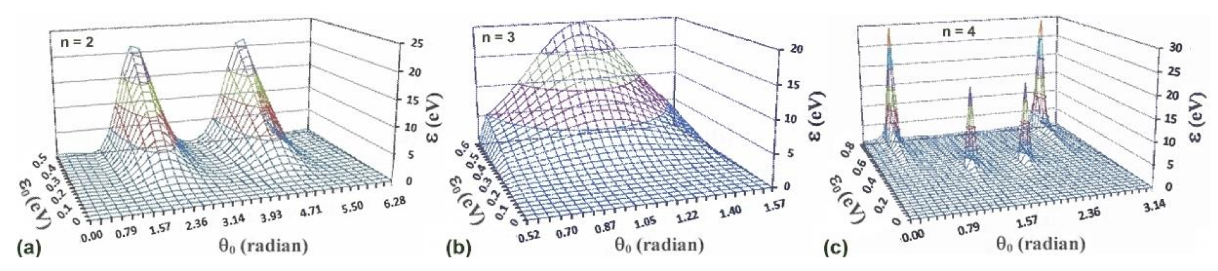
In the numerical evaluations, the parameter values used in the (1) second harmonic case are and the interaction time , where and ; (2) third harmonic case are , and the interaction time , where and ; and (3) fourth harmonic case are , the interaction time , where and , and the explosive time .
The numerical results of the three cases are plotted and presented in Figure 12a–c. As shown, ultra-energetic electrons are generated in all three cases. These ultra-energetic electrons enhance airglow and produce ionizations when colliding with the background neutral particles.
It is realized that the geomagnetic field varies slightly with the altitude and it takes time and interaction length to energize electrons in the resonance interaction. Theoretical results [23] indicate that the excited upper hybrid waves have a frequency bandwidth. In the parametric coupling, the upper hybrid wave frequency is , where is the heating wave frequency and the lower hybrid frequency . In HAARP, the lower hybrid resonance frequency is . For , . Hence, has a bandwidth of 18 kHz, which covers the change of the ionospheric electron gyro frequency over an altitude range of over 10 km. This interaction length is crucial for producing energetic electron flux for ionizations.
The plasma frequency increases faster than the decrease of the gyro frequency in the upward direction. Thus, the resonance interaction region is extended only downward from the upper hybrid resonance layer and with the presence of the downward propagating upper hybrid waves. This explains why the artificial ionization layers descend during their development as observed in electron cyclotron harmonic resonance heating experiments.
6. Production of Artificial Ionization Layer (AIL)
6.1. Down-Going Upper Hybrid Waves and Artificial Ionization Layer (AIL) Location
Upward-propagating upper-hybrid waves reflect at a height near the HF reflection layer (h = hr) to become down-propagating upper hybrid waves. These waves () continuously propagate down from the upper-hybrid resonance layer, , along the geomagnetic field, to a height h, and it evolves to (); its wavevector changes the magnitude and direction (i.e., the oblique angle, , to the geomagnetic field) due to the dropping of the plasma density.
In the propagation, the wave frequency and the horizontal component of the wavevector do not change, i.e., , where θ is the conjugate of the geomagnetic dip angle α ~ 76°, which set up two equations for to be
and
These two equations are solved to obtain , which increases with an increase of and with the decrease of θ as waves propagate down; upper-hybrid waves then convert linearly into oblique propagating Langmuir waves [49].
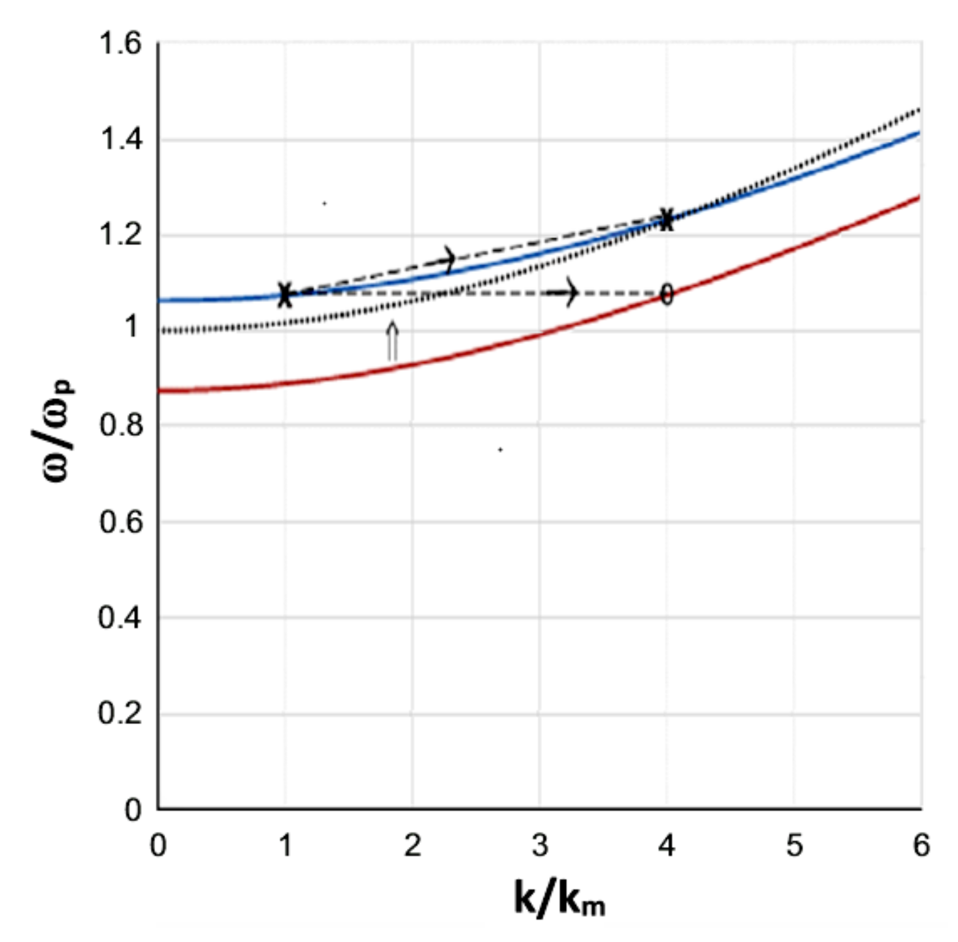
The process is presented in Figure 13, in which the blue curve, , and red curve, are the dispersion curves of the upper-hybrid wave () and the Langmuir wave () at the parametric excitation layer (at ) and at the AIL (at ), respectively, where and is the oblique angle (to the geomagnetic field) of the Langmuir wave at AIL location ().
As the upper-hybrid wave propagates downward, its frequency does not change, but the wavenumber increases and the wavevector inclines toward the magnetic field. As shown in Figure 13, the cross shifts horizontally to the right to the circle (o) on the red curve to become an obliquely propagating Langmuir wave. The downward change of the wave location can also be represented by rescaling the vertical axis by the ratio , which essentially moves the Langmuir wave curve (red curve) up to the dot curve, . The dot curve intersects with the blue curve at a point also marked with a cross (x), which then represents the new mode appearing in the AIL. It shows that the upper-hybrid wave converts to an obliquely propagating Langmuir wave with . Because the horizontal component of the wavevector does not change, i.e., , thus , where is the initial wavenumber of the upper-hybrid wave in a range (). The converted Langmuir wave further cascade if it still has a large amplitude.
6.2. Generation of Energetic Electrons
The excited upper-hybrid and lower-hybrid waves accelerate electrons to higher energy. As the heating wave frequency ramps up, the harmonic cyclotron resonance region moves downward because the electron cyclotron frequency increases with lowering the altitude; thus, the double resonance layer shifts downward for shorter wavelength upper hybrid waves; it extends the generation region of the upper-hybrid waves, and also enhances the harmonic cyclotron resonance interaction between the excited waves and the electrons because shorter wavelength upper-hybrid waves provide stronger finite Larmour radius effect, as discussed in Section 5.
Those electrons at Doppler shifted cyclotron harmonic resonance interaction with the excited waves (i.e., ), can be energized to high energy while moving down along the geomagnetic field if the interaction persists long enough. Constant is assumed because the cyclotron harmonic resonance interaction mainly accelerates the gyration speed of the electron. However, if resonance interaction occurs at , i.e., , where = (), the resonance condition will be detuned as the electron moves downward, and the magnitude |Δω| of the detuning frequency increases with the downward distance. It means that the interaction becomes weaker in time. On the other hand, if at , i.e., by, e.g., 100 kHz, then , where , which is a gain factor; decreases as the electron moves downward with the wave. Hence, the interaction is continuously enhanced, and reaches cyclotron harmonic resonance at , where , and resonant electrons can gain considerable energy from the upper hybrid waves.
The power transfer from wave to the electron moving along the magnetic field, i.e., , depends on the phase of which varies with time due to Δω ≠ 0. Although the phase is distributed randomly from 0 to 2π, there are electrons of appropriate phases that will gain energy from the wave, i.e., > 0 and increases; consequently, Δω decreases to give a positive feedback to enhance wave–electron interaction. When Δω drops to a negative value, the feedback of the interaction becomes negative; thus, a sufficient large is necessary to give adequate positive feedback interaction period for the generation of energetic electrons. On the other hand, if is too large, the initial electron–wave interaction will be too weak to lock in the positive feedback in the interaction, or the available interaction spatial distance will be too short to generate energetic electrons. A frequency ramp-up sweep serves the purpose of setting the proper gain factor for achieving continuous positive feedback during the wave–electron interaction in the available altitude range.
6.3. Spatial Bunching to Buildup Energetic Electrons Density in a Thin Layer for AIL Production
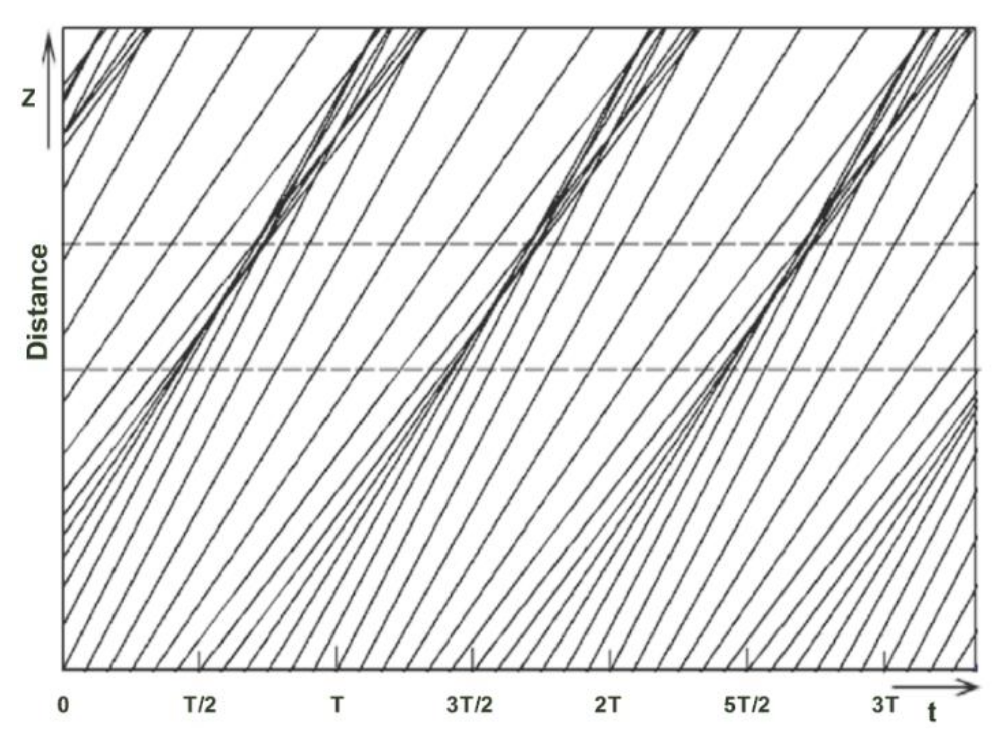
Only a small fraction of electrons in a height layer can achieve cyclotron harmonic resonance with the upper-hybrid waves at ; as the upper-hybrid waves propagate down, more electrons along the path can meet the condition to be in cyclotron harmonic resonance with the upper-hybrid waves. These electrons can bunch together in a layer, where significant ionizations occur to form an AIL.
Because the cyclotron harmonic resonance interaction mainly accelerates the electron gyration speed, constant is adopted to illustrate the bunching phenomenon in Figure 14. As shown, down-going electrons initially located higher with slightly larger initial (or at the same location but starting later), and those located lower with smaller initial (or at the same location but starting earlier), can bunch together at . Although the three bunches between two dash lines in Figure 14 show the accumulation of energetic electrons at three different times, the time delay (difference) of the bunch converts to the spatial difference of the starting location. In essence, Figure 14 also illustrates that groups of energizing electrons starting at different altitudes can bunch together at the same location and time. Such a bunching process builds up the density of energetic electrons at , where an AIL is produced.
7. Nonlinear Plasma Waves
7.1. Nonlinear Schrodinger Equations for the Langmuir Waves and Upper Hybrid Waves
O-mode heating wave passes the upper hybrid resonance layer before reaching the reflection height in an over-dense ionosphere; Langmuir and upper hybrid (electron plasma) parametric instabilities are excited concurrently by the HF heating wave; those waves form standing waves across the magnetic field B0 = − B0 and propagate along the magnetic field (± direction).
7.1.1. Density Irregularities Generated by the Parametrically Excited Electron Plasma Waves
Ponderomotive forces [14,47], induced by the excited Langmuir and upper hybrid (electron plasma) waves, are exerted on electrons; ions follow the electron motion, via the induced self-consistent electric field, to maintain quasi-neutrality. Density irregularities along the geomagnetic field are then generated. The governing equation of plasma density irregularity , driven by the axial component of induced ponderomotive force, is derived as follows.
The continuity and momentum equations are given to be
where and 〈 〉 operates as a mode type filter.
With the aid of (61), (62), and (63) are combined to be
where the electron inertial term is neglected; is the ion acoustic speed, and the ion () mass; and are applied.
Because δne is a non-oscillatory density perturbation, , and (64) is approximated to obtain , where is the electron velocity perturbation by the electron plasma wave field.
7.1.2. Nonlinear Envelope Equation of the Electron Plasma Waves
Only electrons respond effectively to the Langmuir and upper hybrid wave fields, and the formulation involves electron fluid equations (61) and (62), which can be combined to an equation for the electrostatic potential of the electron plasma waves, given by the electron plasma wave field .
The continuity and momentum equations and the Poisson’s equation for the electron plasma wave density, velocity, and electrostatic potential perturbation, , are given to be
where ; the convective term in (66) is separately included in (62). Equations (65) to (67) are then combined to a nonlinear equation for the electron plasma wave potential
where 〈 〉 stands for a filter, which keeps only terms having the same phase function as that of the function on the left-hand side.
Set ., where , , and for Langmuir waves and for upper hybrid waves; from the electron momentum equation, we have
We now neglect the collision, and set and , where B is applied for the two cases: 1) for Langmuir waves and 2) for upper hybrid waves; (68) reduces to
This is a one-dimensional nonlinear Schrodinger equation.
7.2. Analysis
In the following, (70) is analyzed by first converting it to an eigenvalue equation, which is derived by introducing
, where ; (70) becomes
where ; a = ϖ/A and b = B/2A. Consider (ϕ, ξ) as the equivalent spatial coordinate and time of a system, (71) represents an equation of motion of a unit mass object moving in this one-dimensional space and being accelerated by a force of −2(aϕ + bϕ3). Multiply to both sides of (71), it leads to
It is recognized that the quantity in the parenthesis on the LHS of (72) is invariant with . This quantity is the total energy, H, of the object, in which the first term represents the kinetic energy, T, and the second term the potential energy, P. The object is trapped in the potential well ; it moves back and forth in the potential well to have an oscillatory trajectory in the case of H ≠ 0, and a non-oscillatory trajectory in the case of H = 0 and a < 0.
7.2.1. Periodic Solutions
For H ≠ 0, (71) is solved analytically in the cases of
- H > 0 and a > 0
Set , , and , where , (71) is normalized to be
where . The solution of (73a) is a Jacobi elliptic (cosine amplitude) function ; thus,
which is a symmetric alternate function.
- 2.
- H > 0 and a < 0
Again, set , , and , where , (71) is normalized to be
where . (73b) has the same form as (73a), its solution is also a Jacobi elliptic function . Thus,
likewise, it is a symmetric alternate function.
- 3.
- a < 0 and H < 0
Set , , and , i.e., where , (71) is normalized to be
where . The solution of (73c) is a Jacobi elliptic (delta amplitude) function ; thus,
which is a non-alternate periodic function.
7.2.2. Solitary Solution
A localized solution of (71) requires ϕ = 0 = ϕ′ as ; thus H = 0 in the case of a < 0 is considered. Set , , and where , (71) is normalized to be
where . Compare (74) with (73b) and (73c), the solution of (74) is Thus
This is a solitary solution that as
. Its width (∝) is inversely proportional to its amplitude. The cubic nonlinearity of the medium mitigates wave dispersion in the propagation; when the nonlinear effect (∝ square of the amplitude) and the dispersion effect (inversely proportional to the square of the width of the wave packet) reach a balance, a shape-preserved solitary wave is formed and trapped in the self-induced density well (∝ ).
With the aid of (75a), the induced density cavity is given to be
7.3. Discussion
Langmuir waves and Upper hybrid waves are excited by the O-mode HF heater through parametric decay instabilities in HF heating experiments. Those waves are excited in narrow spatial regions below HF reflection layer and the upper hybrid resonance layer, respectively. Artificial density cusps, manifested by bumps in the virtual height spread of the ionogram trace (Figure 2), are induced. The two bumps are in the plasma frequency regions corresponding to the excitation regions of the Langmuir PDI and upper hybrid PDI.
The experimental results also show that the heater caused a significant range spread of the sounding echoes; the range spread was mainly downward, different from the upward spread phenomenon caused by large-scale field-aligned density irregularities. Thus, the observation manifests not only the generation of density ledges signified by bumps expanding the virtual height spread upward, but also the generation of density irregularities along the magnetic field over a large altitude region below the heater-induced density ledges.
The theory and analysis presented in Section 7.1 and Section 7.2 show that the localized Langmuir and upper hybrid waves generated by the HF heater form cavitons near the HF reflection layer and near the upper hybrid resonance layer, which induce bumps in the virtual height spread of the ionogram trace similar to that induced by the density cusp at E-F1 transition layer; incoherent scatter radar (ISR) will be another remote-sensing instrument to diagnose the formation of cavitons, cross checking ionograms’ inference. The down-going Langmuir waves and upper hybrid waves evolve into nonlinear periodic waves propagating along the magnetic field, which backscatter incoherently the sounding pulses to cause downward virtual-height spread.
Funding
This work was supported by the High Frequency Active Auroral Research Program (HAARP), Air Force Research Laboratory (AFRL) at Hanscom AFB, MA, and by the Office of Naval Research, Grant No. ONR-N00014-10-1-0856. Part of the financial support was arranged through NorthWest Research Associates, Inc. under AFRL contract FA8718-08-C-0049.
Acknowledgments
I am grateful to Min-Chang Leeing, MIT, to Brenton Watkins, Univ. Alaska at Fairbanks, to Paul Kossey, AFRL at Hanscom Air Force Base, to Lee Snyder, NorthWest Research Associates, Inc., and to Edward Kennedy, Naval Research Laboratory, for helpful discussions.
Conflicts of Interest
The author declares no conflict of interest.
References
- Gordon, W.E.; Carlson, H.C. Arecibo heating experiments. Radio Sci. 1974, 9, 1041–1047. [Google Scholar] [CrossRef]
- Hagfors, T.; Kofman, W.; Kopka, H.; Stubbe, P.; Äijanen, T. Observations of enhanced plasma lines by EISCAT during heating experiments. Radio Sci. 1983, 18, 861–866. [Google Scholar] [CrossRef]
- Stubbe, P.; Kohl, H.; Rietveld, M.T. Langmuir turbulence and ionospheric modification. J. Geophys. Res. Space Phys. 1992, 97, 6285–6297. [Google Scholar] [CrossRef]
- Kossey, P.; Heckscher, J.; Carlson, H.; Kennedy, E. HAARP: High Frequency Active Auroral Research Program. J. Arctic Res. USA 1999, 1, 1. [Google Scholar]
- Stubbe, P.; Kopka, H.; Dowden, R.L. Generation of ELF and VLF waves by polar electrojet modulation: Experimental results. J. Geophys. Res. Space Phys. 1981, 86, 9073. [Google Scholar] [CrossRef]
- Fejer, J.A. Ionospheric modification and parametric instabilities. Rev. Geophys. 1979, 17, 135–153. [Google Scholar] [CrossRef]
- Showen, R.L.; Kim, D.M. Time variations of HF-enhanced plasma waves. J. Geophys. Res. 1978, 83, 623–628. [Google Scholar] [CrossRef]
- Kuo, S.P.; Lee, M.C.; Djuth, F.T. A new interpretation of plasma-line overshoot phenomena. Geophys. Res. Lett. 1987, 14, 961–964. [Google Scholar] [CrossRef]
- Djuth, F.T. High-resolution observations of HF-enhanced plasma waves at Arecibo. Geophys. Res. Lett. 1990, 17, 1893–1896. [Google Scholar] [CrossRef]
- Kuo, S.P.; Ho, A.Y.; Lee, M.C. temporal evolution of HF-enhanced plasma lines. Geophys. Res. Lett. 1990, 17, 2209–2212. [Google Scholar] [CrossRef]
- Showen, R.L. The spectral measurement of plasma lines. Radio Sci. 1979, 14, 503–508. [Google Scholar] [CrossRef]
- Kuo, S.; Snyder, A. Artificial plasma cusp generated by upper hybrid instabilities in HF heating experiments at HAARP. J. Geophys. Res. Space Phys. 2013, 118, 2734–2743. [Google Scholar] [CrossRef]
- Kuo, S.; Snyder, A.; Lee, M.C. Experiments and theory on parametric instabilities excited in HF heating experiments at HAARP. Phys. Plasmas 2014, 21, 062902. [Google Scholar] [CrossRef]
- Schmidt, G. Physics of High Temperature Plasmas; Elsevier BV: Amsterdam, The Netherlands, 1979; pp. 304–318. [Google Scholar]
- Davidson, R.C. Methods in Nonlinear Plasma Theory. Academic Press: New York, NY, USA, 1972. [Google Scholar]
- Kaufman, A.N.; Stenflo, L. Upper-Hybrid Solitons. Phys. Scr. 1975, 11, 269–270. [Google Scholar] [CrossRef]
- Kuo, S.P.; Brenton, W. Nonlinear upper hybrid waves generated in ionospheric HF heating experiments at HAARP. IEEE Trans. Plasma Sci. 2019, 47, 5334–5338. [Google Scholar] [CrossRef]
- Reinisch, B.W.; Galkin, I.A.; Khmyrov, G.M.; Kozlov, A.V.; Bibl, K.; Lisysyan, I.A.; Cheney, G.P.; Huang, X.; Kitrosser, D.F.; Paznukhov, V.V.; et al. New Digisonde for research and monitoring applications. Radio Sci. 2009, 44. [Google Scholar] [CrossRef]
- Djuth, F.T.; Pedersen, T.R.; Gerken, E.A.; Bernhardt, P.A.; Selcher, C.A.; Bristow, W.A.; Kosch, M.J. Ionospheric Modification at Twice the Electron Cyclotron Frequency. Phys. Rev. Lett. 2005, 94, 125001. [Google Scholar] [CrossRef] [PubMed] [Green Version]
- Kosch, M.J.; Pedersen, T.; Hughes, J.; Marshall, R.; Gerken, E.; Senior, A.; Sentman, D.; McCarrick, M.; Djuth, F.T. Artificial optical emissions at HAARP for pump frequencies near the third and second electron gyro-harmonic. Ann. Geophys. 2005, 23, 1585–1592. [Google Scholar] [CrossRef] [Green Version]
- Kuo, S.P.; Cheo, B.R. Perpendicular electron cyclotron resonance heating by ordinary modes. Phys. Fluids 1981, 24, 778–784. [Google Scholar] [CrossRef]
- Kuo, S.P.; Rubinraut, M. Generation of energetic electrons at second harmonic cyclotron resonance in ionospheric HF heating experiments. Geophys. Res. Lett. 2005, 32. [Google Scholar] [CrossRef]
- Kuo, S.P. Electron cyclotron harmonic resonances in high-frequency heating of the ionosphere. Phys. Plasmas 2013, 20, 092124. [Google Scholar] [CrossRef]
- Rose, G.; Grandal, B.; Neske, E.; Ott, W.; Spenner, K.; Holtet, J.; Måseide, K.; Trøim, J. Experimental results from the HERO Project: In situ measurements of ionospheric modifications using sounding rockets. J. Geophys. Res. Space Phys. 1985, 90, 2851. [Google Scholar] [CrossRef]
- Carlson, H.C.; Wickwar, V.B.; Mantas, G.P. Observation of fluxes of superthermal electron accelerated by HF excited instabilities. J. Atmos. Terr. Phys. 1982, 44, 1089–1100. [Google Scholar] [CrossRef]
- Pedersen, T.; Gustavsson, B.; Mishin, E.; MacKenzie, E.; Carlson, H.C.; Starks, M.; Mills, T. Optical ring formation and ionization production in high-power HF heating experiments at HAARP. Geophys. Res. Lett. 2009, 36. [Google Scholar] [CrossRef]
- Pedersen, T.; Gustavsson, B.; Mishin, E.; Kendall, E.; Mills, T.; Carlson, H.C.; Snyder, A.L. Creation of artificial ionospheric layers using high-power HF waves. Geophys. Res. Lett. 2010, 37. [Google Scholar] [CrossRef] [Green Version]
- Pedersen, T.R.; Holmes, J.M.; Gustavsson, B.; Mills, T.J. Multisite Optical Imaging of Artificial Ionospheric Plasmas. IEEE Trans. Plasma Sci. 2011, 39, 2704–2705. [Google Scholar] [CrossRef]
- Pedersen, T.; McCarrick, M.; Reinisch, B.; Watkins, B.; Hamel, R.; Paznukhov, V. Production of artificial ionospheric layers by frequency sweeping near the 2nd gyroharmonic. Ann. Geophys. 2011, 29, 47–51. [Google Scholar] [CrossRef] [Green Version]
- Pedersen, T.; Reinisch, B.; Paznukhov, V.; Hamel, R. HF propagation characteristics of artificial ionospheric layers. In Proceedings of the 2011 XXXth URSI General Assembly and Scientific Symposium, Istanbul, Turkey, 13–20 August 2011; pp. 1–4. [Google Scholar] [CrossRef]
- Mishin, E.; Pedersen, T. Ionizing wave via high-power HF acceleration. Geophys. Res. Lett. 2011, 38. [Google Scholar] [CrossRef] [Green Version]
- Reinisch, B.W.; Huang, X. Automatic calculation of electron density profiles from digital ionograms, 3, Processing of bottomside ionograms. Radio Sci. 1983, 18, 477–492. [Google Scholar] [CrossRef]
- Galkin, I.A.; Khmyrov, G.M.; Reinisch, B.W.; McElroy, J. The SAOXML 5: New format for ionogram-derived data. In Proceedings of the Fourth Huntsville Gamma-Ray Burst Symposium, Lowell, MA, USA, 27 April–3 May 2007; 974, pp. 160–166. [Google Scholar] [CrossRef]
- Kuo, S.; Snyder, A. Observation of artificial spread-F and large region ionization enhancement in an HF heating experiment at HAARP. Geophys. Res. Lett. 2010, 37. [Google Scholar] [CrossRef]
- Kuo, S.P.; Lee, M.C.; Kuo, S.C. A theoretical model of artificial spread F echoes. Radio Sci. 1985, 20, 546–552. [Google Scholar] [CrossRef]
- Kuo, S.P.; Schmidt, G. Filamentation Instability in Magneto Plasmas. Phys. Fluids 1983, 26, 2529–2536. [Google Scholar] [CrossRef]
- Kuo, S.P.; Djuth, F.T. A thermal instability for the spread-F echoes from HF-heated ionosphere. Geophys. Res. Lett. 1988, 15, 1345–1348. [Google Scholar] [CrossRef]
- Gurevich, V.A. Nonlinear Phenomena in the Ionosphere; Chapter 2; Springer-Verlag: New York, NY, USA, 1978. [Google Scholar]
- Kuo, S.P. Plasma Physics in Active Wave Ionosphere Interaction; World Scientific: Toh Tuck Link, Singapore, 2017. [Google Scholar]
- Perkins, F.W.; Oberman, C.; Valeo, E.J. Parametric instabilities and ionospheric modification. J. Geophys. Res. Space Phys. 1974, 79, 1478–1496. [Google Scholar] [CrossRef]
- Kuo, S.P. Oscillating two-stream instability in ionospheric heating experiments. Phys. Plasmas 2002, 9, 1456–1459. [Google Scholar] [CrossRef]
- Kuo, S.P. Cascade of the parametric decay instability in ionospheric heating experiments. J. Geophys. Res. Space Phys. 2001, 106, 5593–5597. [Google Scholar] [CrossRef]
- Kuo, S.P.; Lee, M.C. Cascade spectrum of HFPLs generated in HF heating experiments. J. Geophys. Res. 2005, 110, 1–7. [Google Scholar]
- Kuo, S.P.; Cheo, B.R.; Lee, M.C. The role of parametric decay instabilities in generating ionospheric irregularities. J. Geophys. Res. Space Phys. 1983, 88, 417. [Google Scholar] [CrossRef]
- Kuo, S.P. The role of nonlinear beating currents on parametric instabilities in magnetoplasmas. Phys. Plasmas 1996, 3, 3957–3965. [Google Scholar] [CrossRef]
- Huang, J.; Kuo, S.P. Cyclotron harmonic effect on the thermal oscillating two-stream instability in the high latitude ionosphere. J. Geophys. Res. Space Phys. 1994, 99, 2173–2181. [Google Scholar] [CrossRef]
- Stenflo, L. Comments on Stimulated Electromagnetic Emissions in the Ionospheric Plasma. Phys. Scr. 2004, 107, 262–263. [Google Scholar] [CrossRef]
- Kuo, S.P.; Lee, M.C.; Kossey, P. Excitation of oscillating two stream instability by upper hybrid pump waves in ionospheric heating experiments at Tromso. Geophys. Res. Lett. 1997, 24, 2969–2972. [Google Scholar] [CrossRef]
- Watkins, B.; Kuo, S.; Secan, J.; Fallen, C. Ionospheric HF Heating Experiment With Frequency Ramping-up Sweep: Approach for Artificial Ionization Layer Generation. J. Geophys. Res. Space Phys. 2020, 125, 1–12. [Google Scholar] [CrossRef]
Figure 1.
Ionospheric heating experiments and some remote-sensing facilities.

Figure 2.
A sequence of ionograms (a–o) showing the evolution of the virtual height spread. Arrows locate the likely bumps in the virtual height spread and the two lines at 2.88 MHz and 3.2 MHz label the plasma frequencies of the upper hybrid resonance layer and high frequency (HF) reflection layer.

Figure 3.
Comparison of ionograms recorded on 16 and 20 November 2009. (a) and (c) Recorded 30 s before the heater turned on and 90 s after the heater turned off; (b) and (d) recorded at the beginning of the moment when the O mode heater turned off.
Figure 3.
Comparison of ionograms recorded on 16 and 20 November 2009. (a) and (c) Recorded 30 s before the heater turned on and 90 s after the heater turned off; (b) and (d) recorded at the beginning of the moment when the O mode heater turned off.

Figure 4.
Ionograms of digisonde echoes recorded on 16 November 2009 during HF heating experiment at High-Frequency Active Auroral Research Program (HAARP). (a) An additional echo trace (pointed by an arrow) appears below the normal echo trace. It signifies artificial ionization structures, and (b) a sequence of seven ionograms recorded from 01:59:40 to 02:03:00 showing the generation and evolution of the artificial ionization structures. Courtesy of Bo Reinisch.

Figure 5.
A pair of ionograms (a) without heating effect and (b) with heating effect; the ionogram in (b) was acquired at the beginning of the moment the heater turned off after the 5.75 MHz O-mode heater turned on for 2 min.
Figure 5.
A pair of ionograms (a) without heating effect and (b) with heating effect; the ionogram in (b) was acquired at the beginning of the moment the heater turned off after the 5.75 MHz O-mode heater turned on for 2 min.

Figure 6.
Electron density distributions at the two recording times.

Figure 7.
(a) The unique echoes (red triangles) extracted from the 21:18 UT ionogram and (black dash) the common echoes of 21:18 UT and 21:22 UT ionograms, recorded during heating experiment conducted on 16 November 2009, and (b) an ionogram showing that the natural cusp near foE (the peak plasma frequency of the ionospheric E region) in the density distribution causes spread of the sounding echoes to also appear as a bump.

Figure 8.
Ray trajectory in a planar stratified medium.

Figure 9.
(a) Field-aligned density irregularity (FAI) geometry and digisonde beam. (b) and (c) Vertically incident ray trajectories of (b) O-mode ray of 2.8 MHz and (c) X-mode ray of 2.8 MHz, in the presence of 0 to 10 % FAI. The axes x and z in (b) and (c) are normalized to k0 = ω0/c.
Figure 9.
(a) Field-aligned density irregularity (FAI) geometry and digisonde beam. (b) and (c) Vertically incident ray trajectories of (b) O-mode ray of 2.8 MHz and (c) X-mode ray of 2.8 MHz, in the presence of 0 to 10 % FAI. The axes x and z in (b) and (c) are normalized to k0 = ω0/c.

Figure 10.
(a) Trajectories of backscatter rays of 3.5 to 4 MHz in the absence of FAI and in the presence of 15% FAIs, (a) o-mode rays and (b) x-mode rays.
Figure 10.
(a) Trajectories of backscatter rays of 3.5 to 4 MHz in the absence of FAI and in the presence of 15% FAIs, (a) o-mode rays and (b) x-mode rays.

Figure 11.
Cascade of down-going and up-going upper hybrid waves, in terms of the wavevector matching condition, over an altitude range is illustrated; (a) cascade to down-going Langmuir sidebands and up-going ion acoustic waves; and (b) cascade to up-going Langmuir sidebands and down-going ion acoustic waves.

Figure 12.
The dependencies of the steady state electron energy ε on the initial energy ε0 and the phase angle θ0 of the initial transverse velocity after acceleration by upper hybrid waves through (a) second harmonic, (b) third harmonic, and (c) fourth harmonic resonance interactions.
Figure 12.
The dependencies of the steady state electron energy ε on the initial energy ε0 and the phase angle θ0 of the initial transverse velocity after acceleration by upper hybrid waves through (a) second harmonic, (b) third harmonic, and (c) fourth harmonic resonance interactions.

Figure 13.
Mode conversion as the upper hybrid wave (the crossing point x on the blue curve) propagates down to becoming a parallel propagating Langmuir wave (the circle o on the red curve) in the artificial ionization layers (AIL) region.
Figure 13.
Mode conversion as the upper hybrid wave (the crossing point x on the blue curve) propagates down to becoming a parallel propagating Langmuir wave (the circle o on the red curve) in the artificial ionization layers (AIL) region.

Figure 14.
Trajectories of electrons with different velocities and starting time at z = 0. Electron bunching as a function of position and time is illustrated.
Figure 14.
Trajectories of electrons with different velocities and starting time at z = 0. Electron bunching as a function of position and time is illustrated.

Publisher’s Note: MDPI stays neutral with regard to jurisdictional claims in published maps and institutional affiliations. |
© 2021 by the author. Licensee MDPI, Basel, Switzerland. This article is an open access article distributed under the terms and conditions of the Creative Commons Attribution (CC BY) license (http://creativecommons.org/licenses/by/4.0/).
Share and Cite
MDPI and ACS Style
Kuo, S. Linear and Nonlinear Plasma Processes in Ionospheric HF Heating. Plasma 2021, 4, 108-144. https://0-doi-org.brum.beds.ac.uk/10.3390/plasma4010008
AMA Style
Kuo S. Linear and Nonlinear Plasma Processes in Ionospheric HF Heating. Plasma. 2021; 4(1):108-144. https://0-doi-org.brum.beds.ac.uk/10.3390/plasma4010008
Chicago/Turabian StyleKuo, Spencer. 2021. "Linear and Nonlinear Plasma Processes in Ionospheric HF Heating" Plasma 4, no. 1: 108-144. https://0-doi-org.brum.beds.ac.uk/10.3390/plasma4010008