Article

Reviewing the Crop Residual Burning and Aerosol Variations during the COVID-19 Pandemic Hit Year 2020 over North India

Department of Earth and Atmospheric Sciences, National Institute of Technology Rourkela, Rourkela 769008, India
*
Author to whom correspondence should be addressed.
Submission received: 1 March 2021 / Revised: 14 June 2021 / Accepted: 29 June 2021 / Published: 1 July 2021

Abstract

:
The north Indian states of Haryana and Punjab are believed to be the key sources of air pollution in the National Capital Region due to massive agricultural waste burning in crop harvesting seasons. However, with the pandemic COVID-19 hitting the country, the usual practices were disrupted. COVID-19 preventive lockdown led to restricted vehicular and industrial emissions and caused the labours to leave the agricultural business in Haryana and Punjab. With the changed scenario of 2020, the present study investigates the variations in air quality over the Haryana and Punjab, and their relative impact on the air quality of Delhi. The work attempts to understand the change in agricultural waste burning during 2020 and its implication on the local air quality over both the states and the transported pollution on the national capital Delhi. The study utilises in-situ data for the year 2019–2020 with satellite observations of MODIS aqua/terra for fire counts, aerosol optical depth (AOD) and back-trajectories run by the hybrid single-particle Lagrangian integrated trajectory model (HYSPLIT).

1. Introduction

Air quality is a global issue that recognizes no boundaries and creates regional weather and climate imbalances due to its strong impact on radiation alterations [1]. The aerosols are considered interactive with meteorological parameters compared to other gaseous pollutants [2]. The higher values of aerosols loading and their imperative interaction between various weather and climate processes over south-east Asia are among the top priorities in the air pollution studies for the past few years to solve the regional to global scale issues [3]. Over the Indian region, the aerosol loading is high, with an identified hotspot region over the Indo-Gangetic plains [4]. These aerosols are crucial for aerosol-cloud-precipitation interactions [5] and change the intensity of precipitation [6], which makes the understanding of aerosol variation more important.
The pre-monsoon season (March–May) is identified with higher heating of the land areas and significant aerosols concentration over northern India [7]. The air quality over the national capital (Delhi) is far too poor by the threshold values defined by the Government of India around the year and is believed to be a result of locally emitted pollutants along with transported ones from the nearby regions [8]. Apart from local emissions of the substantial amount of various air pollutants, the significant contribution in transported air pollution to Delhi is believed to be by the agricultural waste burning from the north-Indian states of Haryana and Punjab in both Rabi and Kharif crop seasons [9,10]. The crop residue burning shows maximum emissions of PM2.5 during winter months (October–November), followed by summer months of April and May over the Indo-Gangetic plains [11,12]. The residual crop burning is a systematic process that has been getting worse over the years [13].
The year 2020 encountered the unfortunate pandemic situation of COVID-19 spread world-wide, with a halt to industrial and transportation sectors due to lockdown for preventing the virus spread and unexpected recovery of air quality globally [14]. The Indian region also benefits from improved air quality [15,16,17], though different regions show improvement in various pollutants by a different magnitude. The pandemic hit year also presents a unique opportunity to understand the background values of various pollutants over different regions in real scenarios [18] and understand the changing patterns of transported pollution over heavily polluted areas in Delhi. To understand the impact of the COVID-19 lockdown (24 March–31 May 2020) over the Indian region, we need to focus on the pre-monsoon season, which marks the harvesting period for the Rabi crops [19]. The published literature confirms that air quality during the COVID-19 lockdown over Delhi has improved significantly [20,21]. In addition, there was a shift in harvesting of Rabi crops due to the migration of farming labours during the lockdown over northern India [22]. Moreover, recent studies suggest a good correlation between higher PM2.5 concentrations to COVID-19 spread over the Indian region [23]. Together, these situations make it an interesting case study to understand how the locally improved air quality over Delhi and shift in agricultural harvesting over Haryana and Punjab are related during the COVID-19 lockdown period.
The present study explores this relationship between the lockdown period air quality improvement over Delhi and the local air quality over Haryana and Punjab with a watch on the residual crop burning during the period. The concentration of air pollutants changes even if emissions are the same depending on changing weather conditions [24]. Weather parameters play critical roles in modulating air pollutants and are considered in all prediction modes for pollutants [25,26]. Therefore, to compare two particular years’ data for any pollutant, one needs to account for different weather conditions. Recently, Shi et al. [24] have proposed the de-weathering technique, based on random forest algorithm proposed by Grange et al. [27], which is able to normalise the weather impacts on pollutants, and provide one-to-one comparisons for any site. The present work utilised the de-weathering technique along with detrending of data sets to remove any biasness involved due to seasonality of meteorological variations. The work attempts to find if the crop burning during the lockdown period changed the air quality over Delhi significantly amid the absence of background pollution from vehicular and industrial emissions.

2. Material and Methods

2.1. Study Area

The study is focused on the northern India states: Punjab, Haryana and Delhi, depicted in Figure 1 with major road, railway, highways network, industrial region and rivers. Punjab is situated in the north-western part of India lies between 29°30′ to 32°32′ N and 73°55′ to 76°50′ E, which covers an area of 50,362 square kilometres with a population of 27 million [28]. The state bordered by the neighbouring country Pakistan in the west, Himachal Pradesh in the north-east, Haryana and Rajasthan in the south and the union territory Jammu and Kashmir in the north. The state has rich alluvial plains with numerous streams and some broad water canal systems. An undulating hill belt connects along the north-eastern portion of the states at the Himalayan foothills. It has a mean height of 300 m AMSL, with 180 m in the south-west and greater than 500 m in the north-east boundary.
Haryana, the land-locked state is located between 27°39′ to 30°35′ N and 74°28′ to 77°36′ E covering an area of 44,212 square kilometres with a population of 25 million [28]. The elevation varies from 200 m to 1200 m ASL. The state has only 4% area covered by forests. The Karoh Peak, the highest peak of Haryana located in the Panchkula district near the Morni hills in the Shivalik hill ranges in the greater Himalayas with an elevation of 1467 m. The state has four topographical landscapes like the Yamuna–Ghaggar plain, the lower Shivalik Mountains, the Bagar tract and the Aravali ranges. The Yamuna River flows through Haryana’s eastern boundary, which is the tributary river of the Ganges.
Delhi, the National Capital, is located in India’s northern part lies between 28°24′ to 28°52′ N and 76°50′ to 77°21′ E. It covers 1484 square kilometres, with a population of about 16.8 million [28]. The city was bordered by different satellite cities like Gurgaon, Faridabad of state Haryana and Noida, Ghaziabad cities of the state Uttar Pradesh (UP). The Yamuna River constructs the eastern border of the area and separates the UP and Punjab. Delhi attributes to a humid subtropical climate (Koppen Cwa) and also a hot and semi-arid (Koppen BSh) climate [29]. Delhi receives an annual rainfall of 714 mm, with the vast majority of which falls in the Monsoon season [30].

2.2. Data and Methodology

The in-situ observations are location specific and one need to use satellite data for complete coverage of the regions. The use of satellite data for the analysis of aerosol transportation and variation is very common for finding the total column loading [31].
The primary data used for this study is the MODIS Level 2 daily Aerosol Optical Depth product of 1 km resolution, which uses the multi-angle implementation of atmospheric correction (MAIAC) algorithm for retrieving aerosol optical depth (AOD) [32,33]. The analysis was performed with green band AOD at 0.55 µm with the Aqua and Terra operational collection for the period 2017–2020 (January–May) over the study region. To support the study variability over pre-COVID period, visible infrared imaging radiometer suite (VIIRS) thermal anomalies from NASA’s Fire Information for Resource Management System (FIRMS) [34,35] was analysed over the study regions from 2017–2020 with the improved spatial resolution of the 375 m using MOD14/MYD14 Fire and Thermal Anomalies algorithm. Relating with the fire anomalies, NDVI of the crop over the region was analysed with the MODIS vegetation indices on daily intervals at a spatial resolution of 500 m using red (620–670 nm) and near-infrared (841–876 nm) bands from Level 2 atmospheric corrected surface reflectance products of Aqua and Terra operational collection [36]. The satellite data has been considered for the whole region (all the districts of Haryana and Punjab) for MODIS fire counts, AOD and NDVI values.
At ground level, inter-comparison and validation with the satellite data are supported by the United States Environmental Protection Agency (US EPA) hourly PM2.5 data of Delhi [37] and Central Pollution Control Board (CPCB) daily PM2.5 data of other reference sites (Amritsar, Ludhiana, Gobindgarh, Faridabad, Gurugram, Rohtak) [38]. The daily data recorded by CPCB used the tapered element oscillating micro balance (TEOM) method for measuring PM2.5 (μ gm−3) [39,40]. The in-situ data of PM2.5 concentration for three representative stations of Punjab (i.e., Amritsar, Ludhiana and Gobindgarh) and three stations of Haryana (Faridabad, Gurugram and Rohtak) for the period 2017–2020 (January–May) have been analysed for the present work. These stations are chosen as representative sites for the states due to heavy pollution load over the year for them and the sites for industrial and agricultural industries associated with them. The average proportion of the satellite data coverage is estimated to be about 96.35% throughout the study period. Specifically, the data for March 2018 and May of 2019 is estimated to have the least coverage of about 92.29% and 91.90%, respectively. To support the study, the northern most flank of the region experiences this missing data and presumed that this trivial fraction of missing data does not affect the overall analysis.
We calculated back trajectory analysis by using National Centres for Environment Prediction (NCEP)/National Centre for Atmospheric Research (NCAR) GDAS (Global Data Assimilation System) 1° data and HYSPLIT version 4 [41,42,43]. For the present work, we have calculated one day (−24 h) isentropic back trajectories (three hourly), supported by the source-apportionment method concentration weighted trajectories (CWT) analysis has been employed in the present study [44]. The back trajectories have been calculated over Delhi to account the transported pollution analysis. The cluster analysis based on the Euclidian distance for the calculated back trajectories have been employed in the present work to find the mean trajectories based on the distance. The data used in the present study has no gaps in the in-situ, reanalysis (GDAS data) or satellite observations of AOD and NDVI, whereas the fire counts are on the event basis.
While comparing the data for a particular year from the previous years for any pollutant, the role of meteorology plays an important role and cannot be ignored. “De-weathering” is one technique, removing the barriers of comparing different years data by removing the influence of meteorological conditions that effect the trend of air quality [45]. De-weathering provides a distinct outline of the air quality trend and the pollutant concentration [24]. This study utilizes de-weathering technique using the random boosted regression tree model using openair r package [46] to isolate the concentration trend in air quality by reducing the recent direct pollutants. It was created with the basic meteorological parameters of temperature, relative humidity, wind speed, wind direction and other influencers as day of the week and week of the year to identify the changes they signify the underlying air quality trend during the lockdown period. Meteorological datasets of temperature, relative humidity, wind speed and direction were collected for the sites other than Delhi from https://app.cpcbccr.com/ccr/#/caaqm-dashboard-all/caaqm-landing (accessed on 26 February 2021) and for Delhi the parameters were acquired from https://www.mosdac.gov.in/aws-time-series (accessed on 26 February 2021). The openair r package is available in https://davidcarslaw.github.io/openair/ (accessed on 12 June 2021).

3. Results

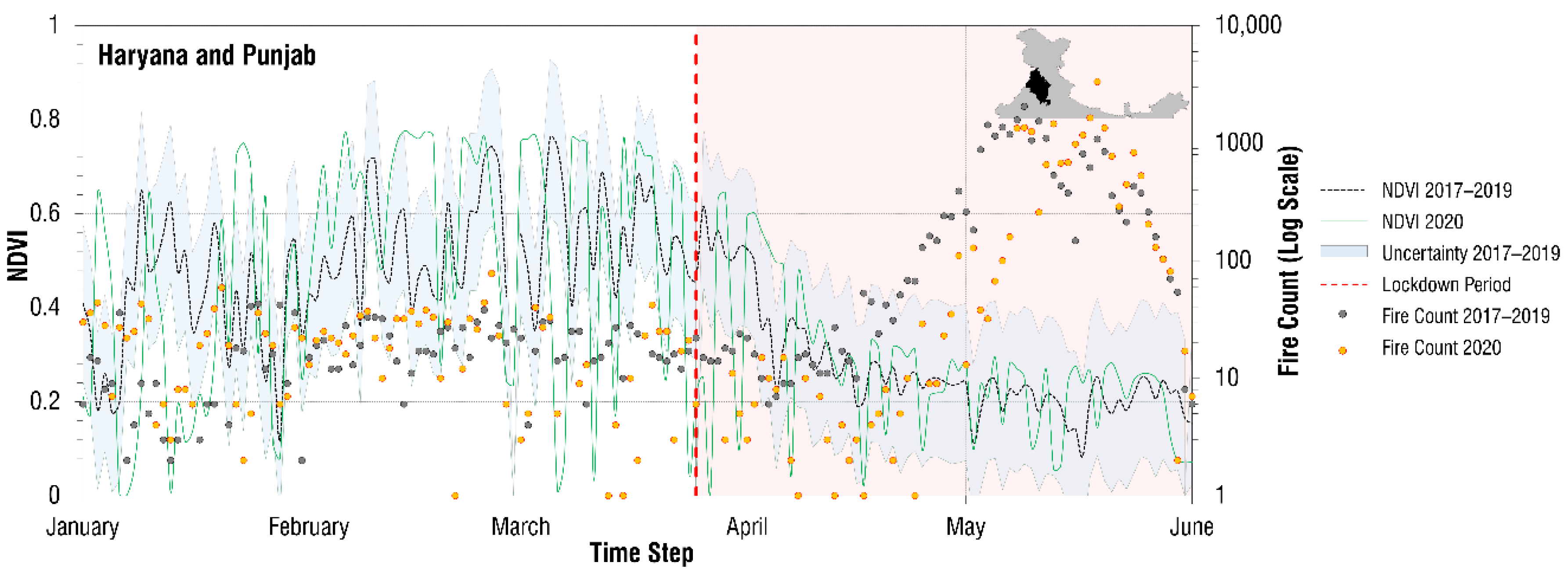
3.1. The Normalized Difference Vegetation Index (NDVI) and Fire Counts over Punjab and Haryana during the Pre-Lockdown and Lockdown Phase

The NDVI has been used for getting the indication of crops over the states of Haryana and Punjab for 2017–2020 along with fire counts as observed by MODIS data for the same period. Figure 2 represents the average fire counts for 2017–2019 and the comparative values for the 2020 period. The lockdown period (i.e., 24 March–31 May 2020) has been masked by red shade starting by the red dotted line in the figure. As one can observe, the fire counts usually increase from the last week of April to May end during Rabi crops harvesting over the region. For 2020, there is a remarkable shift in fire counts, which reaches its peak by the end of May instead of having a peak in the first week of May for 2017–2019. The NDVI values, which are reducing during the same period, confirms the almost constant range during the mid-April to end of May month, which is higher than previous year ranges during May.
Nevertheless, the NDVI variation for 2020 is well within the uncertainty range of 2017–2019. The reduced NDVI values indicate the ripening and harvesting of crops took during the similar period as that of the previous years over Punjab and Haryana; however, in the crop residual burning, there is a remarkable shift during the lockdown period. During the lockdown period, the migration of labours is one primary reason for this anomaly in the fire counts [22]. The results suggest that though NDVI variations are on a similar scale to temporal variations, there is a temporal shift in the fire counts related to crop residual burning, which may impact the pollution loading differently over Delhi.

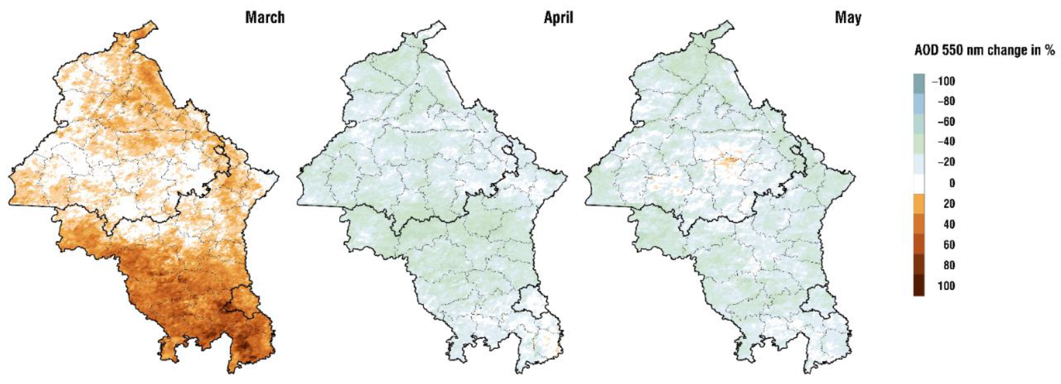
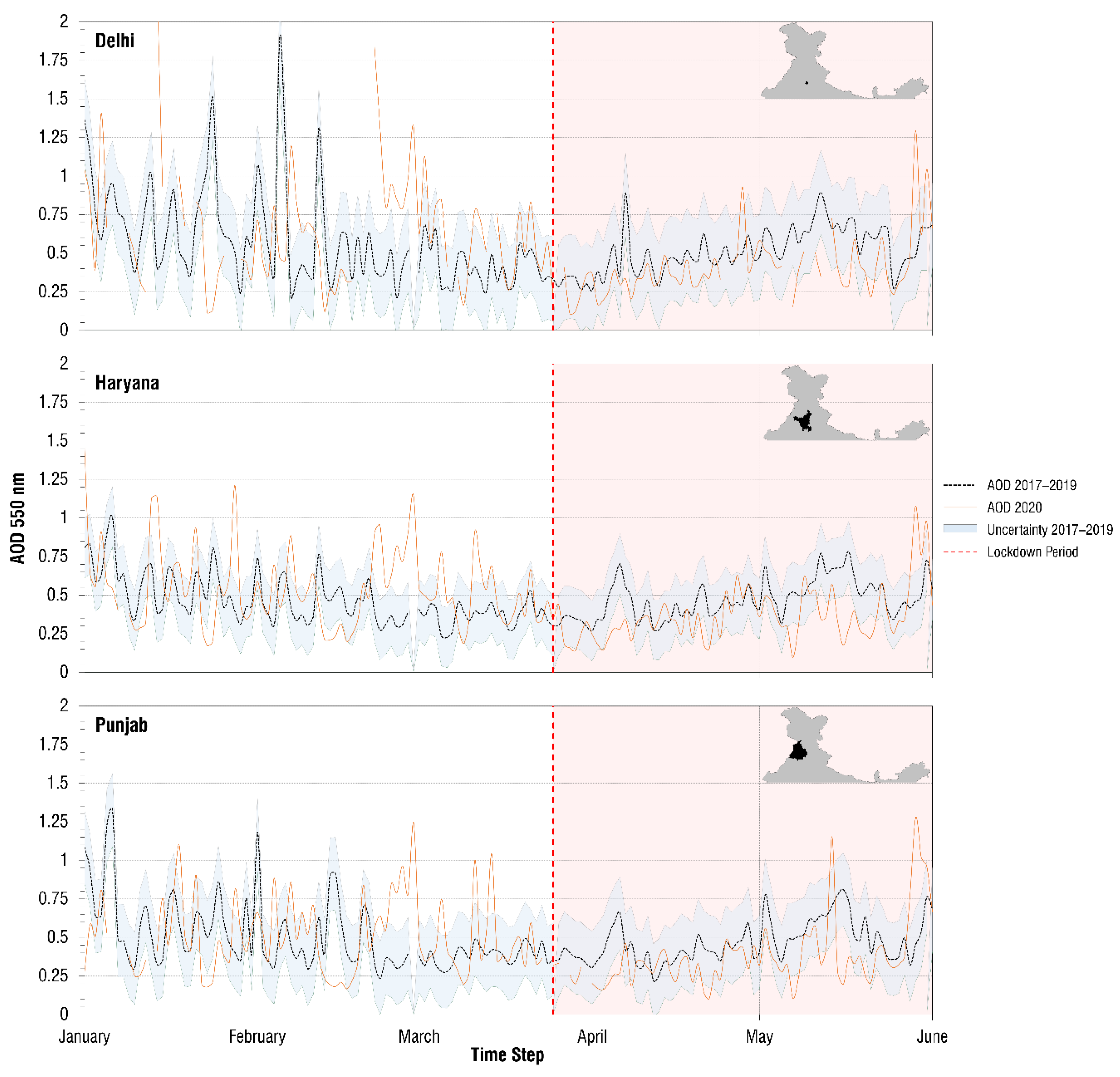
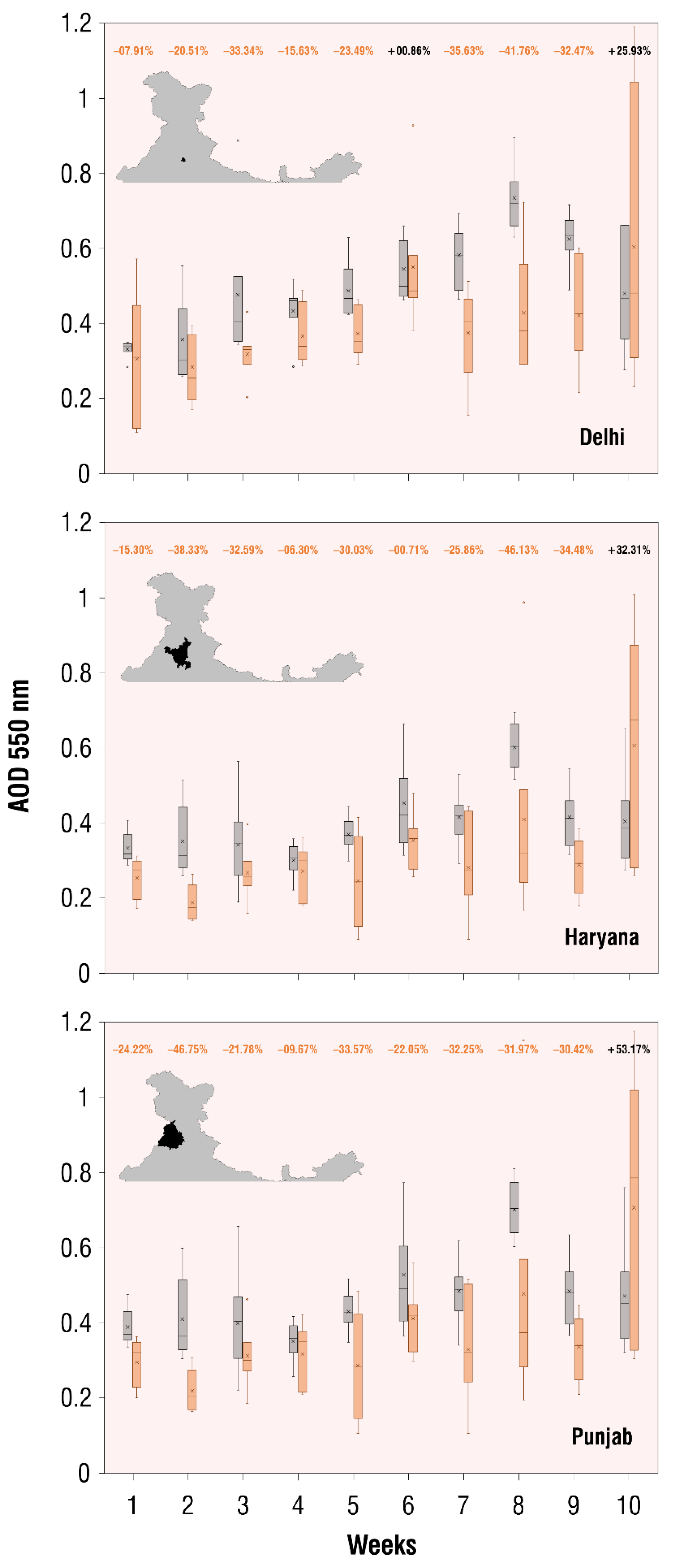
3.2. Variation of PM2.5 and AOD over Punjab, Haryana and Delhi during the Lockdown Phase

To investigate the local scale variations, the in–situ observed PM2.5 values over the study area are analysed for the lockdown period, i.e., 24 March–31 May 2020, and for the same period for 2017–2019. Figure 3 depicts the box–whisker plot for selected stations over the study area to bring out the differences during the lockdown period from previous years. It is to be noted that the data has been de-weathered for all the year to produce the box–whisker diagram shown in Figure 3. The selected sites are based on their spatial location in the study area and depicted by the colour stars in Figure 1. As the meteorological conditions can mask the year wise pollution variation, we used the de–weathering technique [24], as mentioned in the data and methodology section for the datasets shown in Figure 3. Another popular way of removing any possible trends in time series is detrending, which was not changing our datasets in the analysis and thus has not been adopted for the analysis. The results clearly show the decrease in PM2.5 concentrations over all the sites, though the average values of PM2.5 for the whole period does not decrease significantly for Gobindgarh. It is further noted that some stations, as Gobindgarh, Faridabad, Gurugram and Rohtak, though had a sharp decrease in PM2.5 concentrations during the lockdown period, still have higher values of PM2.5 than the daily specified threshold values of 60 µg/m3 [47]. However, the percentage change in PM concentration is ~40% during the lockdown period for whole region, as mentioned by Sharma et al. [48]. The results indicate that for most of the days, the PM2.5 concentrations over the study area are above the threshold values specified by CPCB. The lockdown restriction reduced the vehicular and industrial emissions to zero, but the household cooking; thermal power plants; crop residual burning, and other small-scale activities may be keeping these reduced values on the higher side over the study area [4].
Figure 4 shows the percentage change in AOD values for March, April and May months over the study region. It is evident that March, which experienced the lockdown in the last week (i.e., from 24 March), exhibits a positive percentage change for the study region with higher values over Haryana and Delhi, indicating the increase in pollution load during 2020. The reasons may be twofold: (a) different weather conditions, e.g., weather in 2020 favoring the accumulation of air pollution, and (b) the consideration of whole month of March instead of only lockdown period, so the impact of the lockdown on March is not expected to be massive. The average data coverage for the study period is 96.35%. Further, the difference in the data coverage is less significant which are less than 4.81%—notably, May had the highest difference.
For April, the percentage change shifts to negative values for most regions, indicating the decrease in AOD loading during the lockdown. However, the interesting observation is that some of the areas shows almost no reduction in the AOD percentage change during the lockdown period, and there are some stations of Punjab even experiencing higher AOD loading even during the lockdown period (Bathinda, Sangrur, Barnala and Ludhiana). Such high values during the lockdown phase are mainly associated with various thermal power plants, oil refineries and small-scale industries located in these areas, which were operating even during the lockdown period. Another possibility with the no reduction in April and May is with the association of crop residual burning. As shown in Figure 2, the fire counts are considerably high from the last week of April to the end of May over the region. These burnings may be the reason for the pockets of less reduction or even an increase of AOD values over the study area.
The area-averaged AOD values for Punjab, Haryana and Delhi are also analysed from 1 January–30 June period for 2020 and 2017–2019 average values (Figure 5). The lockdown and post-lockdown (June) period is masked with red colour in Figure 5. The area average values show a substantial decrease in the AOD values for April month, but for May, during the last week, the values are of the same order as previous years or even higher for some cases during the lockdown. To account for the weekly changes in AOD values starting from lockdown day (i.e., 24 March 2020) to the end of lockdown (31 May 2020), we have divided the days to a weekly basis and compared the AOD from the average values of 2017–2019 in Figure 6. The first week consists of 24 March–30 March, second week counts 31 March-06 April and so on, with the last week enclosing 26–31 May 2020. The changes in the percentage were (negative) −00.71% to (negative) −47.75% for the weeks between March to May, indicating a decrease in overall AOD for the lockdown in 2020. However, the changes were positive for the last week of May, ranging from 25.93% to 53.17%, indicating a substantial increase in AOD in 2020 for this week.
The AOD values for June 2020 (post-lockdown) are significantly lower compared to the previous year average for all three states. The average values with no decrease or increase during lockdown periods strongly indicate the impact of crop residue burning over the region, resulting in higher fire counts (Figure 2). However, if we take the average of all the days of lockdown, the reduction in AOD is resulting as stated in various studies [48,49]. The in-situ and satellite observations indicate there is a strong relationship between poor air quality over the study area and crop residual burning during the lockdown period, which is not visible in the total period average values.

3.3. Understanding the Direct Impact of Crop Residual Burning on Transported Air Pollution to Delhi

To further investigate the impact of crop residual burning in Haryana and Punjab on the air quality, we compared the fire counts and PM2.5 in Delhi on specific days. The back trajectory analysis is common approach to find the source regions of transporting air masses [7,50], whereas the CWT analysis proved its suitability in capturing the source regions of transported pollution accurately [44]. Hence, the present study employed back trajectory and CWT analysis over Delhi to find out the source regions, and to correlate the higher pollution days with crop-residual burning events over Haryana and Punjab. To understand the air quality on higher fire count days over Haryana and Punjab, we first identified the days during the lockdown period with higher number of fire count and observed the PM2.5 concentrations over Delhi on the same day and the next day (Table 1). The spatial distance of cities/regions of Punjab varies from ~173–400 km to Delhi. So, for most of the cities of Punjab, dispersion will take 25–48 h with the available wind speed values to reach Delhi. On the other hand, for Haryana, it may be same day transport as well. Though the relation is more complex rather than fire counts over Haryana and Punjab versus Delhi Air quality, we attempted to see if the Delhi air quality shows spike in values with fire counts relation on specific days. It is clear that the PM2.5 concentrations are well above threshold values on the days of high fire counts and even on the following days. Though the values are in the range of average values of PM2.5 concentrations during the lockdown period (Figure 4), it is difficult to relate one to one these fire counts contribution for higher PM2.5 concentrations over Delhi.
For finding the transported pollution impact, we have calculated one day (−24 h) isentropic back trajectories over Delhi using GDAS 1° data by HYSPLIT. Figure 7a shows the trajectories for 2017–2019 over the Indian region. The cluster analysis has been performed based on Euclidian distance for each month and the mean trajectories have been plotted. It is clear that the air masses are directly approaching Delhi in one day, covering most of the districts of Punjab and Haryana. Though there are trajectories approaching from parts of Rajasthan and Madhya Pradesh, the significant contribution is from the states of Punjab and Haryana. To find the possible shift in back trajectory source regions during 2020, the one-day back trajectories are plotted during the lockdown period (Figure 7b). The result shows no major differences in the source regions for the back trajectories reaching Delhi in 2020 from 2017–2019. These back trajectories are widely covering most of the districts of both Punjab and Haryana, and the mean trajectories (clusters) are mostly originating from Haryana and Punjab in both the situations (Figure 7a,b).
To analyse the contribution of transported pollution in Delhi, we employed the source apportionment method; CWT. Figure 7c shows CWT analysis for the 24 March–31 May period during 2017–2020. The higher contribution comes from the districts located in the north-east direction to Delhi, including the districts from Haryana and Punjab: Bhiwani, Rohtak, Jind, Ludhiana, Khanna, Bathinda and Patiala. The states of Haryana and Punjab are home to several agro-based and engineering industries along with two major thermal power plants in Panipat (Haryana) and Bathinda (Punjab) (www.haryana.gov.in; www.punjab.ac.in (1 March 2021)). The oil refinery at Bathinda (Punjab) is also one major industry apart from cement and other small scale establishments over the region. The regions identified by CWT are a combination of industrial and agricultural waste burning regions, contributing to poor air quality over Delhi. Though the lockdown reduces the vehicular emissions significantly with only delivery trucks and medical services vehicles other than specially permitted transport vehicles, the power generation, fossil fuel and crop residual burning contribute to poor air quality in 2020 over the study area. The results suggest that though the area average values might have reduced during the lockdown period, there are many districts in the study area where there were no decreases in aerosol loading due to the aforementioned emission sources. The findings are crucial and contrary to many reports, advocating a constant decrease in aerosol loading over the area (~40%). On the other hand, the results also indicate the existence of higher base levels of aerosols over the study area irrespective of vehicular contributions.

4. Conclusions

The main findings can be summarised as follows:
  • The regulated vehicular and industrial emissions during the COVID-19 lockdown restrictions reduced the air pollution burden in the north Indian states of Haryana, Punjab and Delhi, but the values are still considerably higher and above the threshold.
  • Punjab and Haryana account for the few districts that are not showing any decrease in aerosol concentrations during COVID-19 lockdown. The reason may be attributed to crop residual burning along with various small and medium scale industrial operations in a limited capacity, thermal power plants and oil refinery. The overall reduction during the lockdown period based on spatial average of the region matches with the results reported by other researchers.
  • The aerosol loading over Delhi, though decreased significantly, still remains above the threshold range for most of the days during the lockdown period. The overall air quality is a result of local emissions and possibly considerable contribution from the Punjab and Haryana.
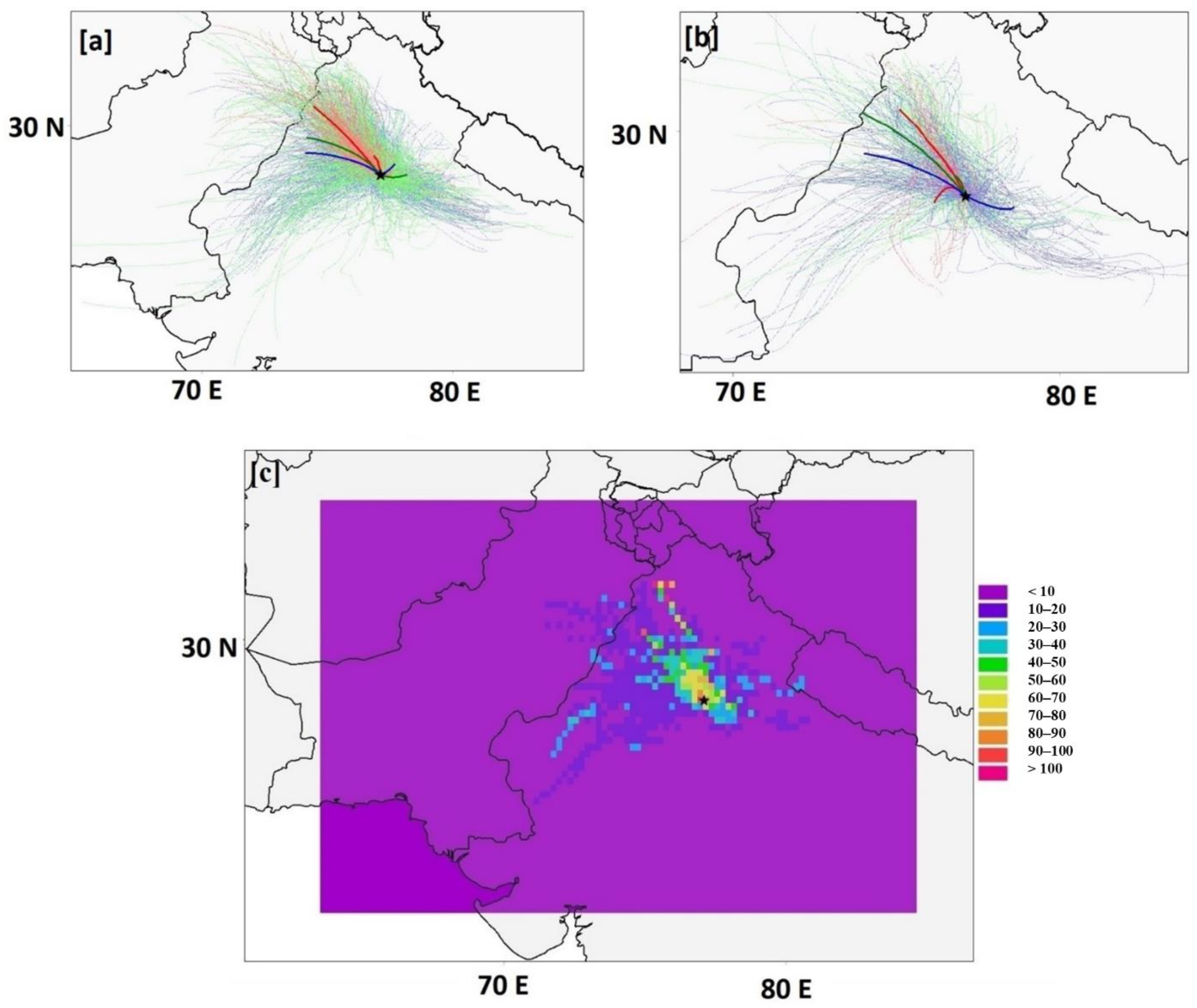
  • The back trajectory and CWT analysis has identified crop residual burning over Haryana and Punjab as one prime activity which was almost unchanged in quantity during the lockdown phase and contributed to the transported pollutants.
Results are showing that despite the restricted industrial and vehicular emissions, the higher than threshold values of PM2.5 exists over Delhi, parts of Haryana and Punjab. The study confirms that crop-residual burning in neighbouring states is one of the main reasons accounting for higher concentrations of PM2.5 in Delhi with a lag of few hours to one day mostly. However, the results are preliminary in nature and need to be studied in-depth concerning chemical composition analysis of emissions and transported pollutants. The overall picture is clear and alarming over the area, with an immediate need of modified policies to control the pollution scenario and reduce the health problems.

Author Contributions

M.H.: software, methodology, writing; R.K.S.: software, methodology; B.T.: conceptualization, methodology, writing, software; R.K.: Data downloading. All authors have read and agreed to the published version of the manuscript.

Funding

This research received no external funding.

Data Availability Statement

Satellite data analysed for the study are freely accessible from https://earthdata.nasa.gov/ (accessed on 1 March 2021) and https://scihub.copernicus.eu/ (accessed on 1 March 2021). The in-situ data used for the study is obtained from https://www.airnow.gov/ (accessed on 26 February 2021) and https://app.cpcbccr.com/ccr/#/caaqm-dashboard-all/caaqm-landing (accessed on 26 February 2021). The GDAS data used for the HYSPLIT Back trajectory model are obtained from ftp://arlftp.arlhq.noaa.gov/pub/archives/gdas1 (accessed on 28 March 2021). The meteorological data for de-weathering has been adopted from https://www.mosdac.gov.in (accessed on 12 June 2021). All other analysed datasets generated for this study are included in the article.

Acknowledgments

Authors would like to gratefully acknowledge the CPCB, AirNow, Copernicus and NASA for providing data sets for carrying out this research work. Authors also want to acknowledge NOAA Air Resource laboratory, and HYSPLIT team for providing the model and Openair package development team for making it available to users. Authors acknowledge the constant efforts of all the public and non-public institutions in tackling the global COVID-19 pandemic.

Conflicts of Interest

The authors declare no conflict of interest.

References

  1. Akimoto, H. Global Air Quality and Pollution. Science 2003, 302, 1716–1719. [Google Scholar] [CrossRef] [Green Version]
  2. Li, Z.; Guo, J.; Ding, A.; Liao, H.; Liu, J.; Sun, Y.; Wang, T.; Xue, H.; Zhang, H.; Zhu, B. Aerosol and boundary-layer interactions and impact on air quality. Natl. Sci. Rev. 2017, 4, 810–833. [Google Scholar] [CrossRef]
  3. Ramanathan, V.; Chung, C.; Kim, D.; Bettge, T.; Buja, L.; Kiehl, J.T.; Washington, W.M.; Fu, Q.; Sikka, D.R.; Wild, M. Atmospheric brown clouds: Impacts on South Asian climate and hydrological cycle. Proc. Natl. Acad. Sci. USA 2005, 102, 5326–5333. [Google Scholar] [CrossRef] [Green Version]
  4. Tyagi, B.; Choudhury, G.; Vissa, N.K.; Singh, J.; Tesche, M. Changing air pollution scenario during COVID-19: Redefining the hotspot regions over India. Environ. Pollut. 2021, 271, 116354. [Google Scholar] [CrossRef]
  5. Choudhury, G.; Tyagi, B.; Singh, J.; Sarangi, C.; Tripathi, S.N. Aerosol-orography-precipitation–A critical assessment. Atmos. Environ. 2019, 214, 116831. [Google Scholar] [CrossRef]
  6. Choudhury, G.; Tyagi, B.; Vissa, N.K.; Singh, J.; Sarangi, C.; Tripathi, S.N.; Tesche, M. Aerosol-enhanced high precipitation events near the Himalayan foothills. Atmos. Chem. Phys. Discuss. 2020, 20, 15389–15399. [Google Scholar] [CrossRef]
  7. Gogikar, P.; Tyagi, B. Assessment of particulate matter variation during 2011–2015 over a tropical station Agra, India. Atmos. Environ. 2016, 147, 11–21. [Google Scholar] [CrossRef]
  8. Ghude, S.D.; Jain, S.L.; Arya, B.C.; Beig, G.; Ahammed, Y.N.; Kumar, A.; Tyagi, B. Ozone in ambient air at a tropical megacity, Delhi: Characteristics, trends and cumulative ozone exposure indices. J. Atmos. Chem. 2008, 60, 237–252. [Google Scholar] [CrossRef]
  9. Jethva, H.; Chand, D.; Torres, O.; Gupta, P.; Lyapustin, A.; Patadia, F. Agricultural Burning and Air Quality over Northern India: A Synergistic Analysis using NASA’s A-train Satellite Data and Ground Measurements. Aerosol Air Qual. Res. 2018, 18, 1756–1773. [Google Scholar] [CrossRef] [Green Version]
  10. Jethva, H.; Torres, O.; Field, R.D.; Lyapustin, A.; Gautam, R.; Kayetha, V. Connecting Crop Productivity, Residue Fires, and Air Quality over Northern India. Sci. Rep. 2019, 9, 16594. [Google Scholar] [CrossRef] [Green Version]
  11. Bray, C.D.; Battye, W.H.; Aneja, V.P. The role of biomass burning agricultural emissions in the Indo-Gangetic Plains on the air quality in New Delhi, India. Atmos. Environ. 2019, 218, 116983. [Google Scholar] [CrossRef]
  12. Sahu, S.K.; Mangaraj, P.; Beig, G.; Samal, A.; Pradhan, C.; Dash, S.; Tyagi, B. Quantifying the high resolution seasonal emission of air pollutants from crop residue burning in India. Environ. Pollut. 2021, 286, 117165. [Google Scholar] [CrossRef]
  13. Jain, N.; Bhatia, A.; Pathak, H. Emission of Air Pollutants from Crop Residue Burning in India. Aerosol Air Qual. Res. 2014, 14, 422–430. [Google Scholar] [CrossRef] [Green Version]
  14. Liu, F.; Wang, M.; Zheng, M. Effects of COVID-19 lockdown on global air quality and health. Sci. Total Environ. 2021, 755, 142533. [Google Scholar] [CrossRef] [PubMed]
  15. Singh, R.P.; Chauhan, A. Impact of lockdown on air quality in India during COVID-19 pandemic. Air Qual. Atmos. Health 2020, 13, 921–928. [Google Scholar] [CrossRef]
  16. Singh, J.; Tyagi, B. Transformation of Air Quality over a Coastal Tropical Station Chennai during COVID-19 Lockdown in India. Aerosol Air Qual. Res. 2021, 21. [Google Scholar] [CrossRef]
  17. Sahu, S.K.; Tyagi, B.; Beig, G.; Mangaraj, P.; Pradhan, C.; Khuntia, S.; Singh, V. Significant change in air quality parameters during the year 2020 over 1st smart city of India: Bhubaneswar. SN Appl. Sci. 2020, 2, 1990. [Google Scholar] [CrossRef]
  18. Beig, G.; Bano, S.; Sahu, S.; Anand, V.; Korhale, N.; Rathod, A.; Yadav, R.; Mangaraj, P.; Murthy, B.; Singh, S.; et al. COVID-19 and environmental -weather markers: Unfolding baseline levels and veracity of linkages in tropical India. Environ. Res. 2020, 191, 110121. [Google Scholar] [CrossRef] [PubMed]
  19. Pal, S.; Chowdhury, P.; Talukdar, S.; Sarda, R. Modelling rabi crop health in flood plain region of India using time-series Landsat data. Geocarto Int. 2020, 1–28. [Google Scholar] [CrossRef]
  20. Mahato, S.; Pal, S.; Ghosh, K.G. Effect of lockdown amid COVID-19 pandemic on air quality of the megacity Delhi, India. Sci. Total Environ. 2020, 730, 139086. [Google Scholar] [CrossRef] [PubMed]
  21. Bray, C.D.; Nahas, A.; Battye, W.H.; Aneja, V.P. Impact of Lockdown during the COVID-19 Outbreak on Multi-Scale Air Quality. Atmos. Environ. 2021, 254, 118386. [Google Scholar] [CrossRef]
  22. Press Information Bureau. The Daily COVID Bulletin. 2020. Available online: https://pib.gov.in/PressReleasePage.aspx?PRID=1628127 (accessed on 10 June 2020).
  23. Sahu, S.K.; Mangaraj, P.; Beig, G.; Tyagi, B.; Tikle, S.; Vinoj, V. Establishing a link between fine particulate matter (PM2.5) zones and COVID -19 over India based on anthropogenic emission sources and air quality data. Urban Clim. 2021, 38, 100883. [Google Scholar] [CrossRef]
  24. Shi, Z.; Song, C.; Liu, B.; Lu, G.; Xu, J.; Van Vu, T.; Elliott, R.J.R.; Li, W.; Bloss, W.J.; Harrison, R.M. Abrupt but smaller than expected changes in surface air quality attributable to COVID-19 lockdowns. Sci. Adv. 2021, 7, eabd6696. [Google Scholar] [CrossRef]
  25. Gogikar, P.; Tyagi, B.; Gorai, A.K. Seasonal prediction of particulate matter over the steel city of India using neural network models. Model. Earth Syst. Environ. 2019, 5, 227–243. [Google Scholar] [CrossRef]
  26. Gogikar, P.; Tripathy, M.R.; Rajagopal, M.; Paul, K.K.; Tyagi, B. PM2.5 estimation using multiple linear regression approach over industrial and non-industrial stations of India. J. Ambient Intell. Humaniz. Comput. 2021, 12, 2975–2991. [Google Scholar] [CrossRef]
  27. Grange, S.K.; Carslaw, D.C.; Lewis, A.C.; Boleti, E.; Hueglin, C. Random forest meteorological normalisation models for Swiss PM10 trend analysis. Atmos. Chem. Phys. Discuss. 2018, 18, 6223–6239. [Google Scholar] [CrossRef] [Green Version]
  28. The Registrar General & Census Commissioner, India. Census. 2011. Available online: http://www.censusindia.gov.in/2011census/population_enumeration.html (accessed on 1 March 2021).
  29. Peel, M.C.; Finlayson, B.L.; McMahon, T.A. Updated world map of the Köppen-Geiger climate classification. Hydrol. Earth Syst. Sci. 2007, 11, 1633–1644. [Google Scholar] [CrossRef] [Green Version]
  30. Planning Department, Government of NCT Delhi. Economic Survey of Delhi (2008–2009); Planning Department, Government of NCT Delhi: Delhi, India, 2009.
  31. Singh, J.; Noh, Y.-J.; Agrawal, S.; Tyagi, B. Dust Detection and Aerosol Properties Over Arabian Sea Using MODIS Data. Earth Syst. Environ. 2019, 3, 139–152. [Google Scholar] [CrossRef]
  32. Lyapustin, A.I.; Wang, Y.; Laszlo, I.; Hilker, T.; Hall, F.G.; Sellers, P.J.; Tucker, C.J.; Korkin, S.V. Multi-angle implementation of atmospheric correction for MODIS (MAIAC): 3. Atmospheric correction. Remote Sens. Environ. 2012, 127, 385–393. [Google Scholar] [CrossRef]
  33. Mhawish, A.; Banerjee, T.; Sorek-Hamer, M.; Lyapustin, A.; Broday, D.M.; Chatfield, R. Comparison and evaluation of MODIS Multi-angle Implementation of Atmospheric Correction (MAIAC) aerosol product over South Asia. Remote Sens. Environ. 2019, 224, 12–28. [Google Scholar] [CrossRef]
  34. Csiszar, I.; Schroeder, W.; Giglio, L.; Ellicott, E.; Vadrevu, K.; Justice, C.O.; Wind, B. Active fires from the Suomi NPP Visible Infrared Imaging Radiometer Suite: Product status and first evaluation results. J. Geophys. Res. Atmos. 2014, 119, 803–816. [Google Scholar] [CrossRef]
  35. Schroeder, W.; Oliva, P.; Giglio, L.; Csiszar, I.A. The New VIIRS 375 m active fire detection data product: Algorithm description and initial assessment. Remote Sens. Environ. 2014, 143, 85–96. [Google Scholar] [CrossRef]
  36. Wang, D.; Morton, D.; Masek, J.; Wu, A.; Nagol, J.; Xiong, X.; Levy, R.; Vermote, E.; Wolfe, R. Impact of sensor degradation on the MODIS NDVI time series. Remote Sens. Environ. 2012, 119, 55–61. [Google Scholar] [CrossRef] [Green Version]
  37. U.S. Environmental Protection Agency. Air Now. 2000. Available online: https://www.airnow.gov/index.cfm?action=airnow.global_summary#India$New_Delhi (accessed on 26 February 2021).
  38. Indian Ministry of Environment. Central Pollution Control Board. Available online: https://app.cpcbccr.com/ccr/#/caaqm-dashboard-all/caaqm-landing (accessed on 26 February 2021).
  39. Allen, G.; Sioutas, C.; Koutrakis, P.; Reiss, R.; Lurmann, F.W.; Roberts, P.T. Evaluation of the TEOM® Method for Measurement of Ambient Particulate Mass in Urban Areas. J. Air Waste Manag. Assoc. 1997, 47, 682–689. [Google Scholar] [CrossRef] [PubMed]
  40. Cyrys, J.; Dietrich, G.; Kreyling, W.; Tuch, T.; Heinrich, J. PM25 measurements in ambient aerosol: Comparison between Harvard impactor (HI) and the tapered element oscillating microbalance (TEOM) system. Sci. Total Environ. 2001, 278, 191–197. [Google Scholar] [CrossRef]
  41. Draxler, R.R.; Hess, G. Description of the HYSPLIT_4 Modeling System NOAA Tech. Memo. ERL ARL-224; NOAA Air Resources Laboratory: Silver Spring, MD, USA, 1997. [Google Scholar]
  42. Draxler, R.R. HYSPLIT4 User’s Guide. NOAA Tech. Memo. ERL ARL-230; NOAA Air Resources Laboratory: Silver Spring, MD, USA, 1999. [Google Scholar]
  43. Stein, A.F.; Draxler, R.R.; Rolph, G.D.; Stunder, B.J.B.; Cohen, M.D.; Ngan, F. NOAA’s HYSPLIT Atmospheric Transport and Dispersion Modeling System. Bull. Am. Meteorol. Soc. 2015, 96, 2059–2077. [Google Scholar] [CrossRef]
  44. Cheng, I.; Zhang, L.; Blanchard, P.; Dalziel, J.; Tordon, R. Concentration-weighted trajectory approach to identifying potential sources of speciated atmospheric mercury at an urban coastal site in Nova Scotia, Canada. Atmos. Chem. Phys. Discuss. 2013, 13, 6031–6048. [Google Scholar] [CrossRef] [Green Version]
  45. Munir, S.; Coskuner, G.; Jassim, M.; Aina, Y.; Ali, A.; Mayfield, M. Changes in Air Quality Associated with Mobility Trends and Meteorological Conditions during COVID-19 Lockdown in Northern England, UK. Atmosphere 2021, 12, 504. [Google Scholar] [CrossRef]
  46. Carslaw, D.C.; Ropkins, K. openair—An R package for air quality data analysis. Environ. Model. Softw. 2012, 27–28, 52–61. [Google Scholar] [CrossRef]
  47. CPCB (Central Pollution Control Board). National Ambient Air Quality Standards (NAAQS); Gazette Notification; CPCB: New Delhi, India, 2009. [Google Scholar]
  48. Sharma, S.; Zhang, M.; Anshika; Gao, J.; Zhang, H.; Kota, S.H. Effect of restricted emissions during COVID-19 on air quality in India. Sci. Total Environ. 2020, 728, 138878. [Google Scholar] [CrossRef]
  49. Jain, S.; Sharma, T. Social and Travel Lockdown Impact Considering Coronavirus Disease (COVID-19) on Air Quality in Megacities of India: Present Benefits, Future Challenges and Way Forward. Aerosol Air Qual. Res. 2020, 20, 1222–1236. [Google Scholar] [CrossRef]
  50. Gogikar, P.; Tyagi, B.; Padhan, R.R.; Mahaling, M. Particulate Matter Assessment Using In Situ Observations from 2009 to 2014 over an Industrial Region of Eastern India. Earth Syst. Environ. 2018, 2, 305–322. [Google Scholar] [CrossRef]
Figure 1. The map of study area (Haryana, Punjab and Delhi) with major road, railway, highways network and rivers in the region along with the industrial region (as stated in the legend). The seven sites where the in-situ observations of PM2.5 have been analysed are marked with different color stars, as mentioned in the legends.
Pollutants 01 00011 g001
Figure 2. The NDVI variations for the period 2017–2019 and 2020 with respect to fire counts (MODIS) over the study region. The lockdown period is masked with red colour.
Pollutants 01 00011 g002
Figure 3. The box–whisker diagram for the variation of in-situ PM2.5 values over Delhi, three stations of Punjab (Amritsar, Ludhiana and Patiala) and three stations of Haryana (Faridabad, Gurugram and Rohtak). The data has been de-weathered for the comparison following Shi et al. [24].
Pollutants 01 00011 g003
Figure 4. The percentage change in AOD variation (MODIS AQUA/TERRA combined, 1 × 1 km, 550 nm) over the study region for the pre-monsoon months (March–May) for 2020 from the average values of 2017–2019.
Pollutants 01 00011 g004
Figure 5. The area averaged AOD variation (MODIS AQUA/TERRA combined, 1 × 1 km) for the period 2017–2019 and 2020 for Delhi (first row), Haryana (second row) and Punjab (third row). The respective locations of the region on the map of India are marked in the inset and the lockdown period is masked with red colour.
Pollutants 01 00011 g005
Figure 6. The box–whisker diagram of variation of AOD values over Delhi, Haryana and Punjab (area averaged) from 24 March–31 May on weekly basis. Area averaged AOD for 2017–2019 is represented by grey and 2020 by orange.
Pollutants 01 00011 g006
Figure 7. The isentropic one day (−24 h) three hourly back trajectories for 24 March–31 May for (a) 2017–2019; (b) 2020 (the lockdown period). The red color trajectories indicate March, green color indicated April and blue color indicates May. Thin lines represent the trajectories and thick lines represent clusters based on Euclidian distance. (c) The CWT analysis for the 24 March–31 May (2017–2020). The black star indicates the position of Delhi, point of origin for these calculations.
Pollutants 01 00011 g007
Table 1. The fire counts (>50) days in Punjab and Haryana during lockdown period and the associated PM2.5 concentrations on same and next day over Delhi.
DatePunjab Fire CountsHaryana Fire CountsDelhi PM2.5 (µg/m3) Same DayDelhi PM2.5 (µg/m3) Next Day
29 April 20202786137139
1 May 20206664150103
5 May 20206634120141
6 May 20201312814189
7 May 2020106927589121
8 May 20201004361121143
9 May 20201036221143116
10 May 202024711116121
11 May 202060452121119
12 May 20201102358119155
13 May 202063046155129
14 May 2020357329129122
15 May 2020672312122145
16 May 20201020154145163
17 May 20201359286163161
18 May 20202923407161161
19 May 20201108238161137
20 May 2020659117137120
21 May 202026130120151
22 May 202037867151139
23 May 202076172139123
24 May 202044190123133
25 May 202014858133130
26 May 202010921130120
27 May 2020958120108
28 May 20206516108789
Publisher’s Note: MDPI stays neutral with regard to jurisdictional claims in published maps and institutional affiliations.

