A Method to Derive the Characteristic and Kinetic Parameters of 1,1-Bis(tert-butylperoxy)cyclohexane from DSC Measurements

Abstract

A differential scanning calorimetry (DSC) experiment was carried out to determine the thermal characteristics of harmful substances. Most experimenters only use the results of measurement and rarely conduct in-depth research on the variety of information behind the measurement. This study used Wolfram’s Mathematica as a DSC measurement research tool to plot the peak curve and derive the characteristic parameters graphically for 1,1-Bis(tert-butylperoxy)cyclohexane. The research steps included raw data cleansing, peak curve normalization, characteristic parameter derivation, and total reaction heat calculation. The kinetic parameters of individual data were derived through the Borchardt and Daniels method, and the autocatalytic model was also verified. We applied the derived characteristic parameters to simulate the peak curve through the Gaussian curve model, which can be used for estimating the peak curve of other heating rates. The derived kinetic parameters were used to observe the effects on the peak curve. The simulation can be used to plan the test results at other rates in a similar temperature range and can also be used to explore the influence of different kinetic parameters on the configuration of the shape of the peak curve and a preliminary model test of materials for materials DSC research.

1. Introduction

Organic peroxides (OP) have been widely applied in the chemical industry since the twentieth century, often in the form of a catalyst such as an initiator, cross-linking agent, or oxidizer because of their specific functional group, the oxygen–oxygen (O–O) bond [1]. The object hazard material of this study was a commercial OP material: 1,1-Bis(tert-butylperoxy)cyclohexane (BTBPC).

BTBPC is an asymmetrical difunctional peroxide (two sets of symmetrical O–O bonds) with low volatility and yellowish liquid formation [2]. It is usually applied as an initiator during the styrene polymerization process to generate a lower residual styrene content and a higher degree of polymerization, mainly used for polystyrene in Taiwan’s chemical plants. In thermal analysis research, the experimental data analysis commonly used in academia is mainly carried out through the following two methods: through software attached to the instrument and software in a related domain [3]. However, to use these professional software packages, we need to understand the relevant knowledge involved in the operation of each software, which means that professionals are needed to operate it. The experimenter acquires only a series of data analyzed by software, and we can only trust these data. Therefore, for situations where we want to study the knowledge within the original test data in detail, a feasible method is to design our own computer languages or use an existing mathematical software package to perform the data analysis and present the results in graphics and tables. Another reason is that a laboratory accumulates numerous test data, but it is only to be archived in the computer’s directory, and no one will likely reuse it. These big data are a type of resource [4,5,6,7] and worthy of putting effort into to enhance our knowledge. In this study, Wolfram’s Mathematica [8] software was adopted to convert data into graphics, and its dynamic interactive functions were applied for real-time editing. Data input, parameter derivation, table, graph creation, and output were completed in the same software interface. The substance studied was the commercial material 1,1-bis(tert-butylperoxy)cyclohexane (BTBPC). It is an asymmetrical bifunctional peroxide, with volatility, light yellow liquid [9], usually used as an igniter in styrene polymerization to produce a lower residual styrene content and a higher polymerization rate; the test data were taken from the laboratory’s DSC database. The method of extracting characteristic parameters followed the steps described in the section of differential scanning calorimetry in “Practice of Thermal Analysis” [10], and Mathematica was used to convert data into peak curves and extract characteristic parameters based on this. The method comprises the following steps: (1) converting the original peak curve into a normalized peak curve through the generated baseline, (2) calculating the intersection point between the baseline and the edge tangent of the curve for obtaining the characteristic temperature, such as onset temperature (T₀), extrapolated temperature (T_p-ext), end set temperature (T_end), full width at half maximum (FWHM) temperature, and total heat of reaction (ΔH_d) by integrating the area under the peak curve. For the derivation of the kinetic parameters, we referred to the steps described in the international standard ASTM E2041 (Borchardt and Daniels) method, and linear model fitting function to calculate pre-reference factor (A), appearance activation energy (E_a), and reaction order (n) for individual data set. The peak curve simulation could be accomplished using the Gaussian curve method, nth order, and auto-catalytic models using the derived characteristic parameters. The simulation results showed compliance with the original peak curve. The procedures used in this study can be applied to the DSC data research [11,12,13,14] of other substances in the laboratory, and simulations can also help us plan further measurements at other rates of a similar temperature range.

2. Materials and Methods

The DSC measure data were collected by testing 70 mass% BTBPC in an iso-paraffin hydrocarbon solvent, which was purchased directly from ACE Chemical Corp., Taiwan. It was stored in a refrigerator at 4 °C to maintain its stability and keep it away from any unexpected heat exposure. It is a low volatility, yellowish liquid peroxy ketal peroxide. The test equipment was a Mettler TA8000 system with an extra pure nitrogen purge and the differential scanning calorimetry (DSC), a DSC821^e instrument with high pressure, gold-plated measuring test crucible (Mettler ME-00026732) [15] was used, along with STARe software to obtain thermal curves. The DSC is the prevailing thermoanalytical device that is used to detect the temperature difference between the sample and reference. First, the DSC has to be blank stabilized for at least half an hour. Then the sample crucible is put onto the heating plate and started. After the test, the crucible mass is measured again to verify no leakage during the experiment. To assess the sensitivity of thermal equilibrium [16,17], we used low heating rates in the dynamic mode of operation with nitrogen (50 mL min⁻¹) as the carrier gas. About 4.5–5.2 mg of the sample was used for acquiring the experimental data. The temperature rise range for each test was to be from 30 to 300 °C.

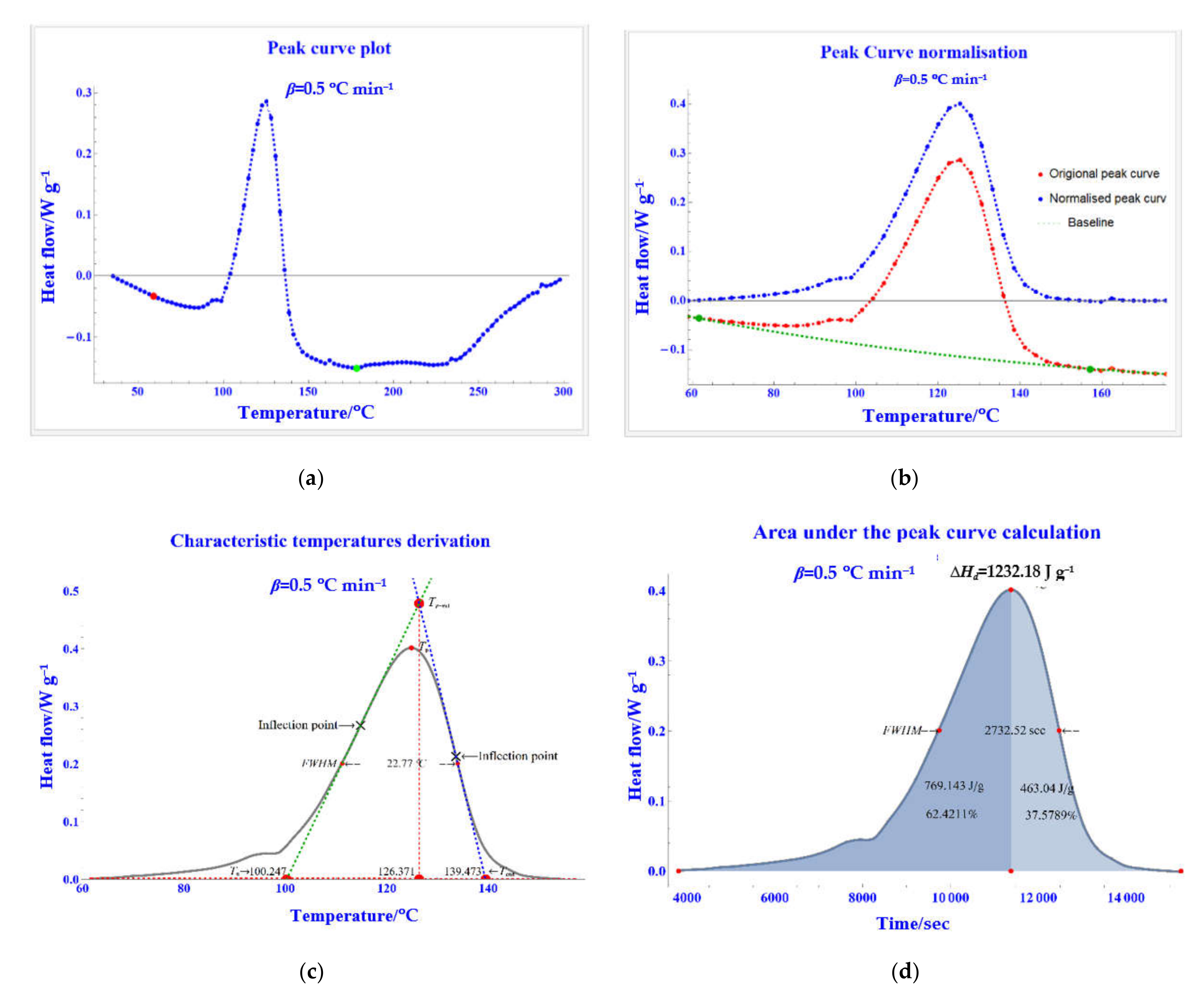
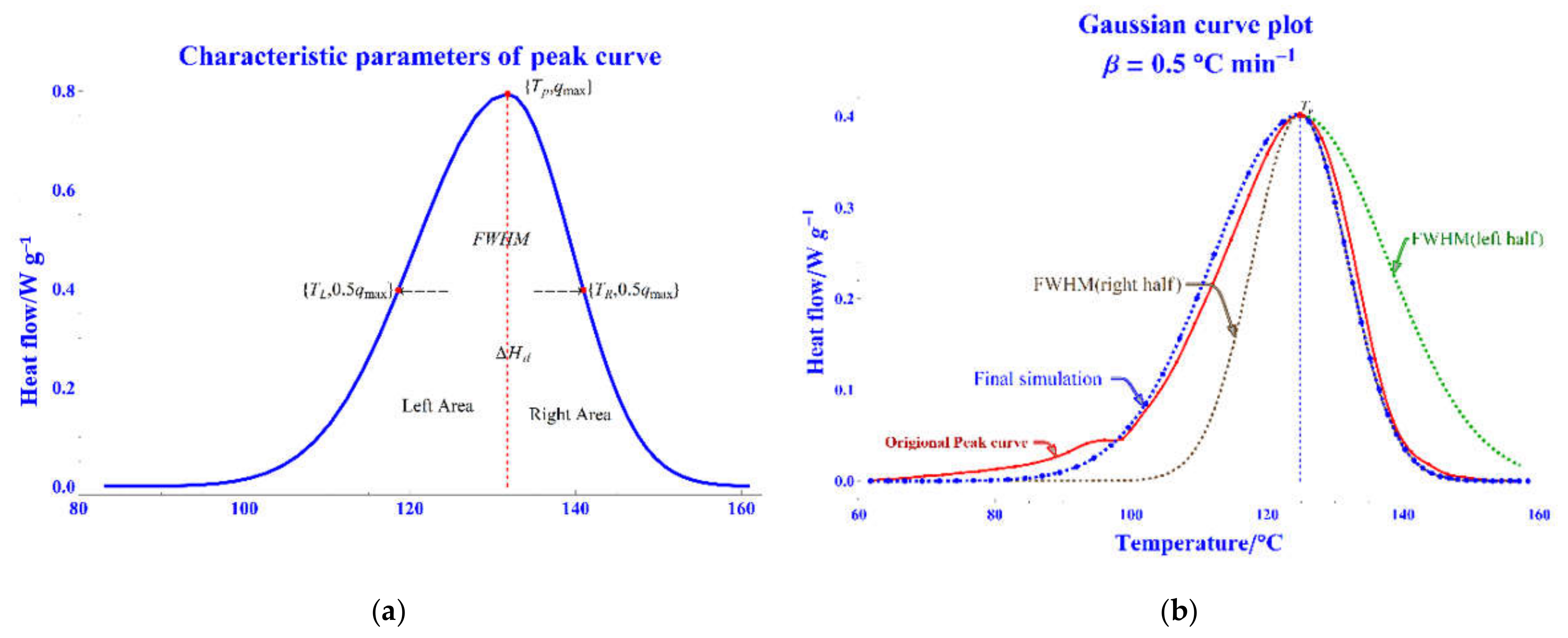
2.1. Calculating Characteristic Parameters from Recovered Peak Curve Data

Software procedures recovered the tested information, and the derived results were compared with the original data to assess their similarity. There were 0.5, 1, 2, 4, 6, 8, and 10 °C min⁻¹ seven low heating rate (β) DSC data, and samples weighed 4.5–5.2 mg. The overall procedure was first to derive characteristic parameters and then calculate the kinetic parameters. DSC peak curve recovery procedures involved data cleaning, peak curve recovery, peak curve normalization, characteristic temperature calculation, and total reaction heat calculation. Before applying the original data to Mathematica software, the original data were subjected to data cleansing to ensure the consistency of the loaded data schema prior to their application in Mathematica software. Figure 1 shows that the original data contains two pieces of information: peak curve-related data and analysis result from STAR^e. The time (t), sample temperature (T_S), and heat flow (value) fields were read into the program for processing.

Figure 2a shows the peak curve recovery process, in which the upward recovery curve illustrates that the process is an exothermic reaction. The graph selected the temperature range through the manipulate [18] function. The primary graphics processing method used the manipulate function to obtain the optimal solution. Figure 2b shows the selection of the spline type and the start and endpoints of the baseline to form the normalized peak curve [19]. In Figure 2c, the inflection points on both sides of the peak curve are calculated first. Then the intersection points between the baseline and the tangent on both sides are intended to obtain the characteristic temperature of T₀, T_end, T_p-ext, T_p, and FWHM temperature. Finally, in Figure 2d, we integrated the area under the peak curve with time to achieve ΔH_d and the ratio of the left to right composition with the centerline.

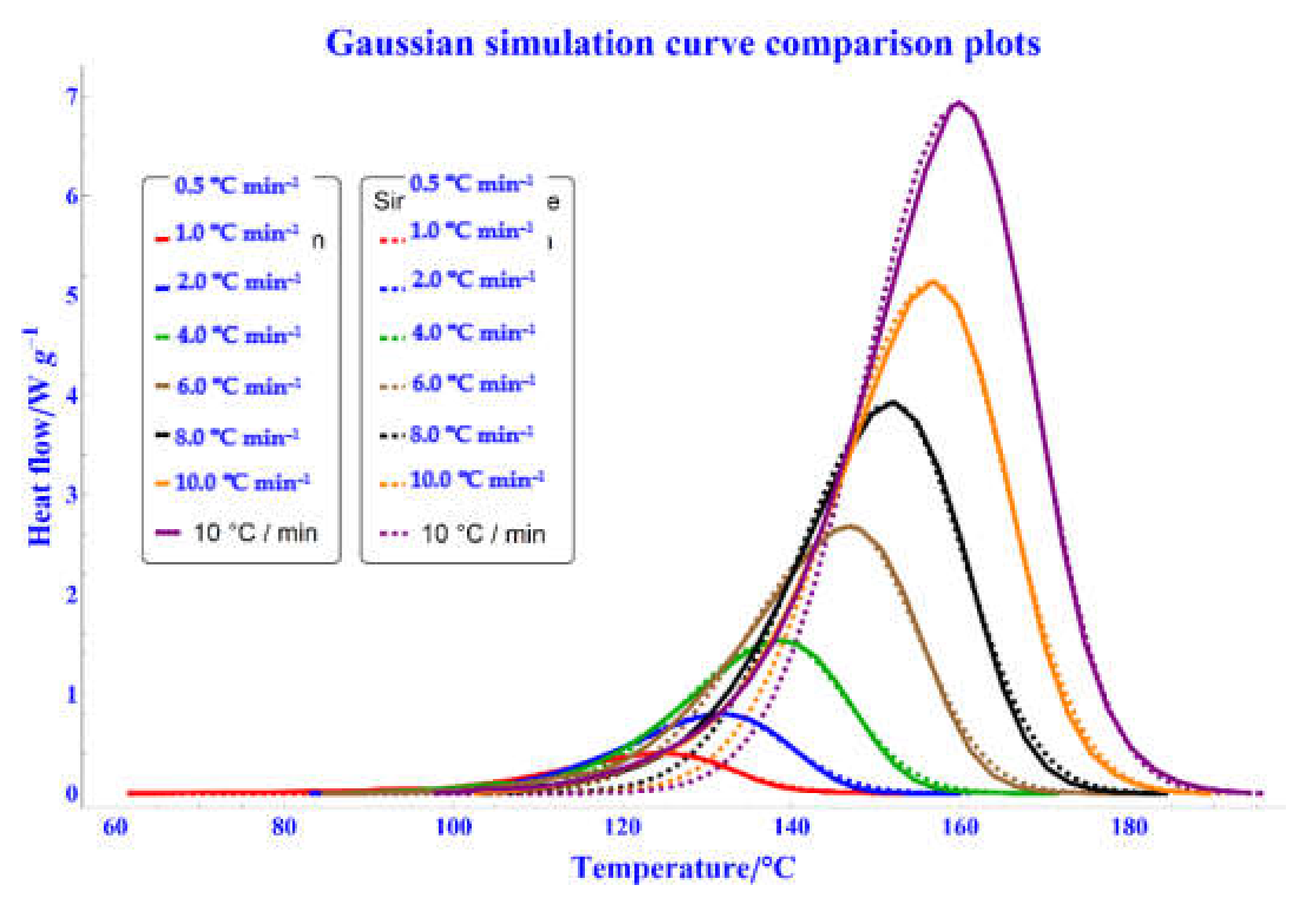
Forming Peak Curve Using the Characteristic Parameters

A simulation model of a peak curve may represent a practical desktop method for assessing reactive chemical hazards because it can offer an easy method of conducting a first evaluation prior to performing a complete experimental investigation. For example, a Gaussian curve could be used as an approximate method of a simple DSC peak curve [20]; only three thermal parameters are required: the peak height (q_max), T_p and the FWHM, as illustrated in Figure 3a. Equation (1) presents the function of the Gaussian curve and portrays the distribution of the Gaussian curve after the loading of temperature data, as formulated in Equation (1).

$$\begin{array}{l}f(T)=q_{\max }\exp (\frac{-{(T-T_{\mathrm{p}})}^2}{2{\sigma }^2})\\ \alpha \cong \frac{1}{2.3548}FWHM\end{array}$$

(1)

Since the peak curve is asymmetric, we simulated two Gaussian curves with double values of the left and right half-peak and extracted the left and right halves of the corresponding Gaussian curves to form the full peak curve, respectively, as shown in Figure 3b.

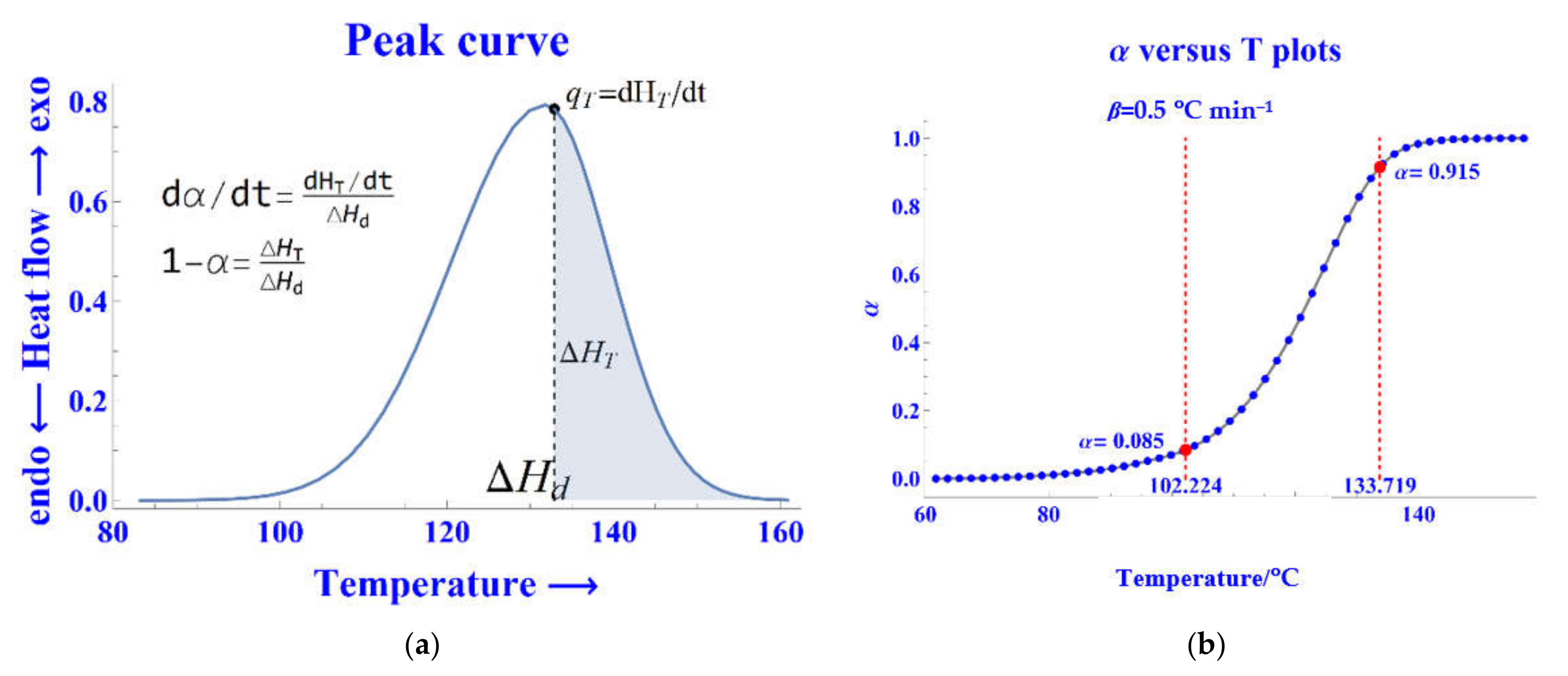
2.2. Calculating Kinetics Parameters of nth-Order Model from a Single DSC Measurement

A formal chemical reaction can be described in a simple form [21] which include the reactant (R), the process time (t), the process temperature (T), the normalized conversion percentage of the reaction (α), and the Product (P) that is de-scribed as Equation (2):

$$R\stackrel{t,T,\alpha }{\to }P$$

(2)

The basic kinetic equation can describe the reaction in derivative form where the rate constant k(T) is represented the dependency of the reaction rate on temperature, and the reaction model of the mechanism function f(α) as Equation (3):

$$\frac{\mathrm{d}\alpha }{\mathrm{d}t}=k(T)f(\alpha )$$

(3)

The temperature dependence of the reaction rate constant, K, is described by the Arrhenius equation [22] where the pre-exponential factor(A) is represented the rate constant at infinite temperature, and the universal gas constant(R) as Equation (4):

$$k(T)=A{e}^{–E_{\mathrm{a}}/RT}$$

(4)

Since the k(T) is the temperature dependence of the reaction rate, we find the relationship between k(T) and T by Equation (4) by taking in the logarithmic form as shown Equation (5):

$$\ln k(T)=\ln A-\frac{E_{\mathrm{a}}}{RT}$$

(5)

Taking Equation (3) in the logarithmic form, the value of lnk(t) can be calculated by Equation (6):

$$\ln k(T)=\ln (\frac{\mathrm{d}\alpha }{\mathrm{d}t})-\ln f(\alpha )$$

(6)

To resolve kinetic parameters from a single DSC measurement, we can use the method described in ASTM E2041, also known as the Borchardt and Daniels (B/D) method [23,24,25,26]. The process derives the kinetic parameters of the E_a, A, n, and the reaction model f(α) = (1 − α)ⁿ [27,28]. The thermal parameters of the peak curve, such as heat flow (dH_T/dt), specified temperature (T), and heat of decomposition, remained at T (ΔH_T), ΔH_d, and the conversion degree at T (ΔH_T/ΔH_d), are as shown in Figure 4a. The ΔH_d value can be calculated by integrating the area under the peak curve. The temperature range from the starting point to the end point can be divided into 50 equal parts. The curve area from the starting point temperature to the peak value of each temperature range point T_i can be defined. Divide the value of the curve area by ΔH to obtain the degree of conversion α_i and link it with the temperature of the segment point T_i to form the record as shown in Figure 4b. Convert the {T, α} record into the T-α function to calculate the corresponding temperatures of α = 0.1 and α = 0.9; afterwards, create 50 equal segments between these temperature intervals also.

Each fraction area of each interval of T_i was then determined, and the corresponding heat flow qi was calculated using Equations (7) and (8) as follows:

$$(1-{\alpha }_{T_{\mathrm{i}}})=\frac{\Delta H_{T_{\mathrm{i}}}}{\Delta H_{\mathrm{d}}}$$

(7)

$$\frac{\mathrm{d}{\alpha }_{T_{\mathrm{i}}}}{\mathrm{d}t}=\frac{q_{T_{\mathrm{i}}}}{\Delta H_{\mathrm{d}}}$$

(8)

Equation (9) was combined from Equations (6) and (8) in logarithmic form of f(α) = (1 − α)ⁿ:

$$\ln k(T_{\mathrm{i}})=\ln (\frac{q_{T_{\mathrm{i}}}}{\Delta H_{\mathrm{d}}})-n\ln (1-{\alpha }_{T_{\mathrm{i}}})$$

(9)

The next step was to plot lnk(T) versus 1/T, with an initial value of n = 1, and sliding it to adjust the value of n, as shown in Figure 5. The straight line is the result of a linear regression calculated using the LinearModelFit [29] function of lnk(T_i) versus 1/T_i. As n is adjusted, the plot on the righthand shows the DSC measured peak curve and the superposition of the simulated peak curve instantly. The simulated peak curve is plotted by fitting the {T, α} record (Figure 4b) with Equation (10) that is combined from Equations (3) and (8):

$$q_{T_{\mathrm{i}}}=\frac{\mathrm{d}{\alpha }_{T_{\mathrm{i}}}}{\mathrm{d}t}\Delta H_d=k(T_{\mathrm{i}}){(1-{\alpha }_{T_{\mathrm{i}}})}^n\Delta H$$

(10)

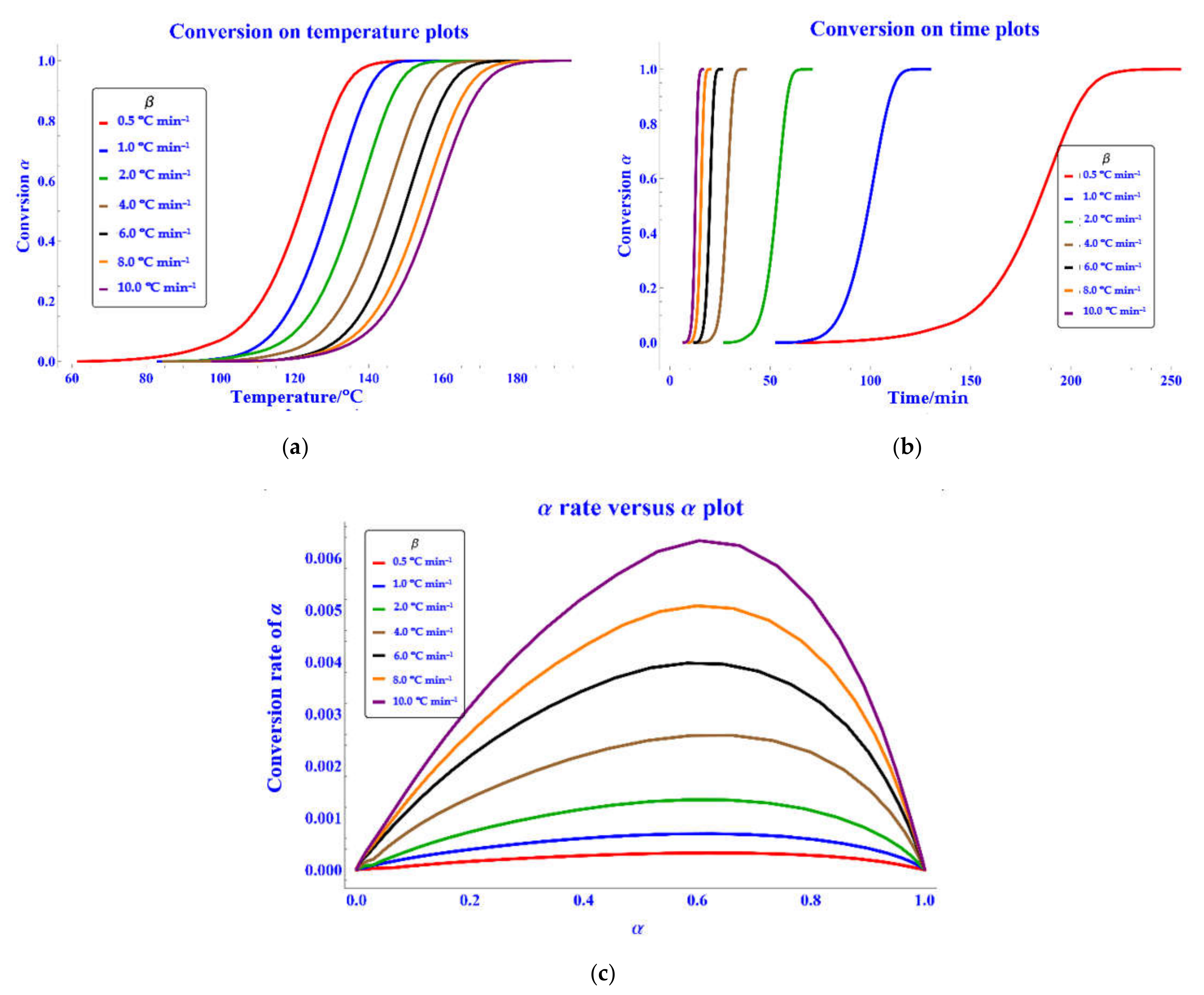
2.2.1. Simulations Using nth-Order Kinetic Parameters

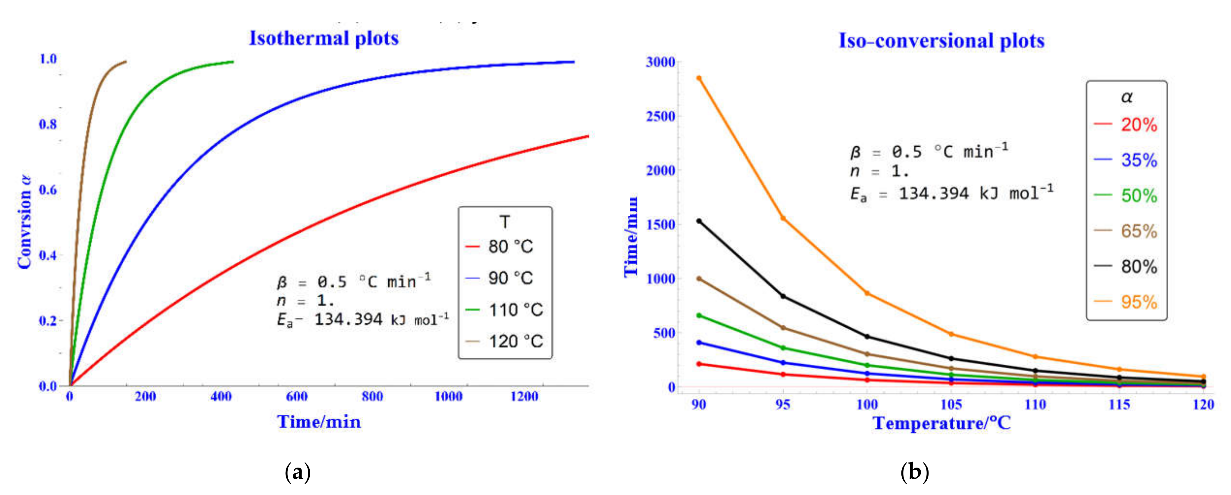
Isothermal Simulations

In theoretical terms, two predictive curves can be obtained from B/D kinetic modelling: the isothermal curve and isoconversional curve. The isothermal curve provides time conditions and degree of conversion information for unique isothermal temperatures [16,30,31]. There are two considerations to obtain acceptable results from the B/D method. First, no mass loss occurs during the reaction. Second, the heating rates are not exceeding 10 °C min⁻¹.

From Equation (2), the conversion function is set as f(α) = (1 − α)ⁿ, and the equation is rearranged as Equation (11):

$$f{\left(\alpha \right)}^{-1} \mathrm{d}\alpha =k(T) \mathrm{d}t$$

(11)

Integrate both sides and set g(α) as integrated form of f(α)⁻¹ as Equation (12):

$$g(\alpha )={\displaystyle \underset{0}{\overset{\alpha }{\int }}\frac{1}{{(1-\alpha )}^n}\mathrm{d}\alpha }=k(T){\displaystyle \underset{0}{\overset{t_{\alpha }}{\int }}\mathrm{d}t}$$

(12)

The right hand of the integrated format can be solved numerically, as Equation (13) shows:

$$t_{\mathrm{i}}=\frac{g({\alpha }_{\mathrm{i}})}{k(T_{\mathrm{j}})}$$

(13)

where k(T_j) is the linear equation derived from the outcome of Equation (9), T_i is the reaction time corresponding to the conversion α_i, and T_j is the chosen isothermal temperature between 10–20 °C below the onset temperature and the intermediate peak temperature [12].

Isoconversional Simulations

The isoconversional curve provides time conditions and temperature information for a specific degree of conversion [16,32,33,34]. Equation (14) delineates the relationships between conversion reaction and specified conversion level through isoconversional simulation:

$$t_{\mathrm{i}}=\frac{g({\alpha }_{\mathrm{j}})}{k(T_{\mathrm{i}})}$$

(14)

where k(T_i) is the linear equation derived from the outcome of Equation (9), T_i is the reaction corresponding to the temperature, and α_j is the specific conversion level.

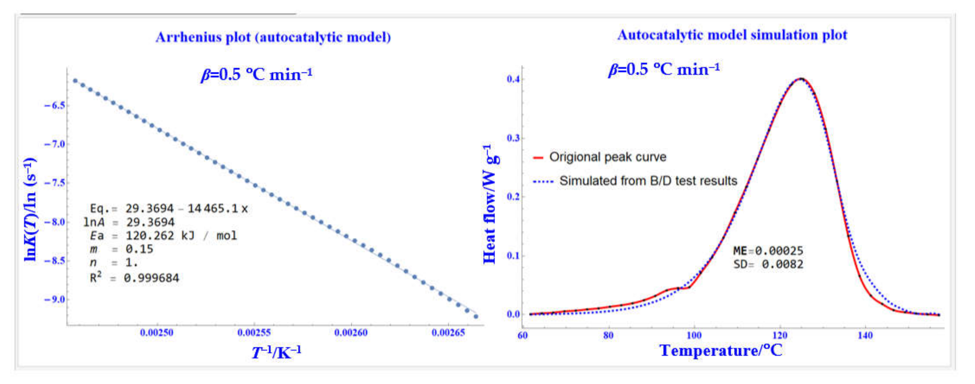
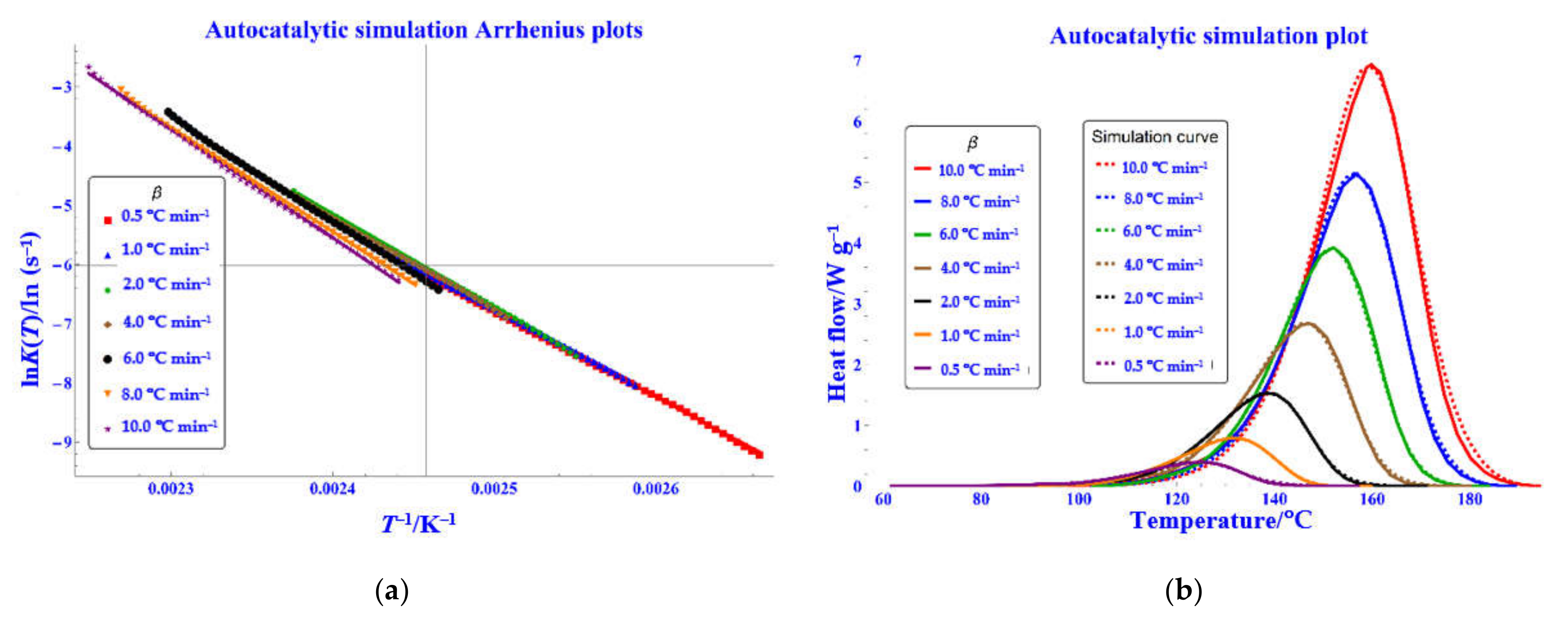
2.3. Calculating Kinetics Parameters of the Autocatalytic Model from a Single DSC Measurement

An autocatalytic model of chemical reaction can be described in the form [21] as illustrated by Equation (15):

$$R+P\stackrel{t,T,\alpha }{\to }2P$$

(15)

The reaction model would be in the form of f(α) = α^m(1 − α)ⁿ [20,35,36,37,38,39]. Combine Equations (6) and (8) in logarithmic form of f(α) = α^m(1 − α)ⁿ into Equation (16):

$$\ln (\frac{\mathrm{d}\alpha }{\mathrm{d}t})=\ln k(T)+\ln ({\alpha }^m{(1-\alpha )}^n)$$

(16)

Combine from Equations (6) and (8) in logarithmic form of f(α) = α^m (1 − α)ⁿ into Equation (17):

$$\ln k(T_{\mathrm{i}})=\ln (\frac{q_{T_{\mathrm{i}}}}{\Delta H})-m\ln {\alpha }_{T_{\mathrm{i}}}-n\ln (1-{\alpha }_{T_{\mathrm{i}}})$$

(17)

Plot lnk(T) versus 1/T, with an initial value of m = 0.5 and n = 1 sliding it to adjust the value of m and n, as shown in Figure 6. The straight line is the result of a linear regression calculated using the LinearModelFit [29] function of lnk(T_i) versus 1/T_i. As n is adjusted, the plot on the right-hand shows the DSC measured peak curve and the superposition of the simulated peak curve instantly. The simulated peak curve is plotted by fitting the {T–α} record (Figure 4b) with Equation (10) that is combined from Equations (3) and (8):

$$q_{T_{\mathrm{i}}}=\frac{\mathrm{d}{\alpha }_{T_{\mathrm{i}}}}{\mathrm{d}t}\Delta H=k(T_{\mathrm{i}}){\alpha }_{T_{\mathrm{i}}}{}^m{(1-{\alpha }_{T_{\mathrm{i}}})}^n\Delta H$$

(18)

2.4. Calculating nth Order Kinetics Parameters from Multiple DSC Measurements

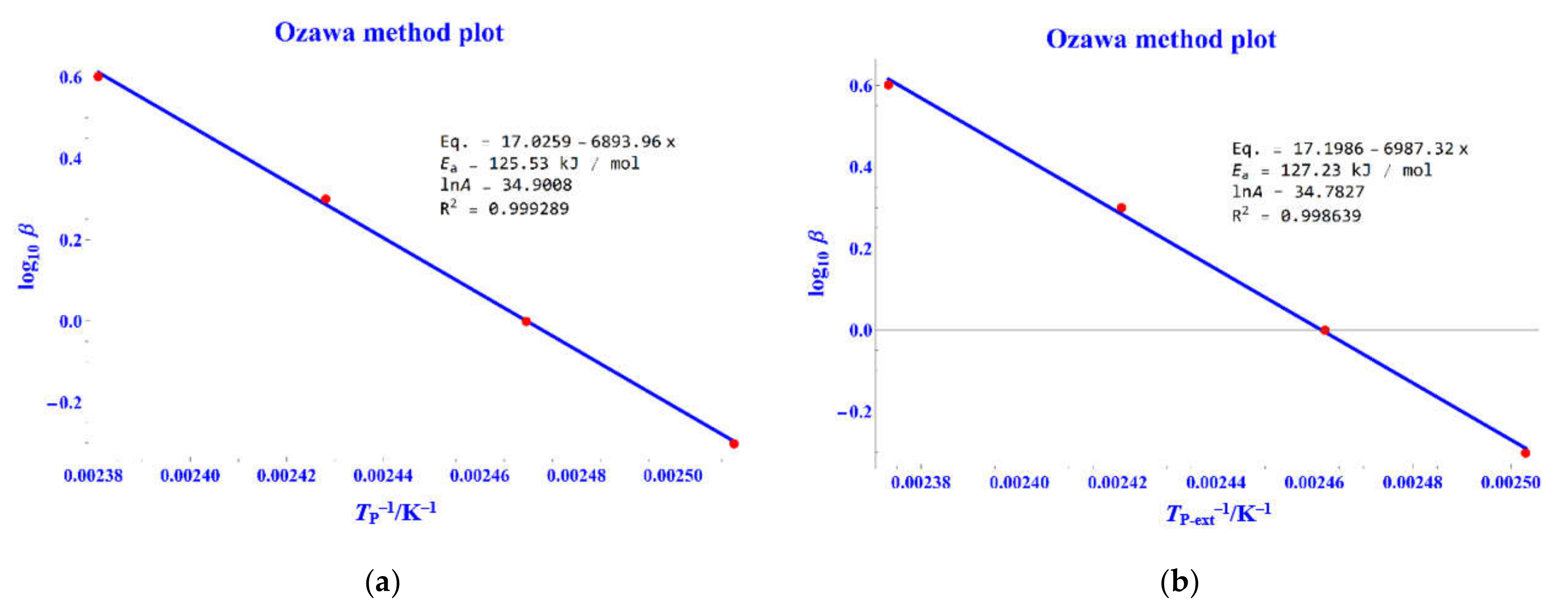
2.4.1. ASTM698 and Flynn/Wall/Ozawa Method

The ASTM E698 method adopts multiple DSC test data to determine the overall kinetic parameters of the exothermic reaction [40,41], under the assumption that the reaction order equals one. This technique is suitable for reactions in which behavior can be described by the Arrhenius equation and the general rate law. The β from the recovery data for this study were 0.5, 1.0, 2.0, and 4.0 °C min⁻¹, which the reaction order was calculated by B/D test and was equal to one already. The next step was to plot log₁₀ β_i (heating rate, K min⁻¹) versus T_Pi, where T_Pi is the maximum temperature in Kelvin. Furthermore, the T_Pi, the T_P-exti is used in calculation also. The four sets of data were subjected to regression analysis via the LinearModelFit function, where the E_a is determined from the slope value of the plot Equation (19) and the A is computed by Equation (20):

$$E_{\mathrm{a}}\cong – 2.19 R(\frac{\mathrm{d}{\log }_{10}\beta }{\mathrm{d}(\frac{1}{T})})$$

(19)

$$A=\frac{\beta E_{\mathrm{a}}{e}^{\frac{E_{\mathrm{a}}}{RT}}}{R{T}^2}$$

(20)

2.4.2. ASTM2890 and the Kissinger Method

ASTM E2890 is a method adopted to determine the apparent activation energy from multiple test data under the assumption that the order of reaction is equal to one [42,43]. The rate of exothermic heat generated by the chemical reaction is proportional to the rate of reaction and measured according to temperature and time. Recovered data with 0.5, 1.0, 2.0, and 4.0 °C min⁻¹ rates were utilized for the same reason as ASTM E698. The test data were employed to plot ln[β_i/T_Pi²] versus 1/T_Pi, where T_Pi is the maximum temperature in Kelvin. The T_Pi, T_P-exti were used in calculation also. The LinearModelFit function was used to assess E_a from the slope value of the plot by Equation (21) and lnA by Equation (22):

$$E_{\mathrm{a}}=-R(\frac{\mathrm{d}\ln (\frac{\beta }{T^2})}{\mathrm{d}(\frac{1}{T})})$$

(21)

$$\ln A=\ln \frac{AR}{E_{\mathrm{a}}}-\ln \frac{R}{E_{\mathrm{a}}}$$

(22)

3. Results

3.1. Derived Characteristic Parameters

In this study, seven heating rate DSC measurements (0.5, 1, 2, 4, 6, 8, and 10 °C min⁻¹) were collected and plotted to peak curves by Mathematica as shown in Figure 7a. The normalized peak curve of heat flow versus temperature or time is shown in Figure 7b,c.

Table 1. Differences of characteristic parameter on temperatures between Mathematica calculated data and DSC measurement of BTBPC. (The numbers in red represent the values derived by this study that were significantly different from the DSC measurements).

β/°C min−1	Source	T0/°C	TP/°C	TP–ext/°C	Tend/°C	FWHM/°C	FWHM/s
0.5	Calculated	100.250	124.840	126.370	139.470	22.770	2732.522
	DSC measurement	122.980	124.580	129.030	136.590	19.890
1	Calculated	108.270	131.770	132.990	146.620	22.350	1340.775
	DSC measurement	111.530	131.630	132.930	144.660	20.170
2	Calculated	115.100	138.690	139.930	153.750	22.480	674.230
	DSC measurement	115.870	138.680	139.850	153.420	22.030
4	Calculated	121.890	146.840	148.190	162.090	23.400	351.192
	DSC measurement	121.950	146.920	148.050	162.230	23.600
6	Calculated	128.470	151.900	153.380	167.950	23.030	230.393
	DSC measurement	128.550	151.890	153.300	167.890	23.110
8	Calculated	132.490	156.760	158.040	173.580	23.570	176.835
	DSC measurement	132.720	156.720	157.980	173.530	23.700
10	Calculated	135.880	159.870	160.970	177.080	23.270	139.399
	DSC measurement	135.750	159.860	160.930	177.230	23.510
Total difference	Mean Error	−3.857	0.056	−0.314	0.713	0.694
	Standard deviation	8.404	0.111	1.035	1.207	1.291

compares the calculated values of the normalized peak curve and the DSC measurement values in terms of characteristic temperature. A positive average error indicates that the calculated value is higher than the experimental value. The T₀, T_end, and T_P-ext are calculated from the intersection of the baseline and the curve tangents. The peak temperature T_p occurs at the point of maximum heat flow q_max. The value of FWHM represents the intersection midpoint of the maximum heat flow on both sides of the peak curve, which is related to the shape of the peak curve. The red letter represents the source of the main difference.

Table 2. Differences of characteristic parameter on heat between Mathematica calculated data and DSC measurement of BTBPC. (The numbers in red represent the values derived by this study that were significantly different from the DSC measurements).

β/°C min−1	Source	qmax/W g−1	△Hd/J	Left Area	Right Area	L/R Area Ratio
0.5	Calculated	1.81	1232.183	0.624	0.376	1.661
	DSC measurement	1.51	802.100	0.577	0.423	1.366
1	Calculated	3.65	1141.903	0.611	0.389	1.568
	DSC measurement	3.1	821.820	0.600	0.401	1.497
2	Calculated	7.98	1133.963	0.610	0.390	1.566
	DSC measurement	7.7	1034.600	0.605	0.395	1.530
4	Calculated	13.4	1031.033	0.606	0.394	1.539
	DSC measurement	13.38	1020.990	0.605	0.395	1.532
6	Calculated	18.8	984.570	0.570	0.430	1.326
	DSC measurement	18.83	979.760	0.570	0.430	1.325
8	Calculated	23.6	1011.177	0.572	0.428	1.338
	DSC measurement	23.6	1003.300	0.571	0.430	1.328
10	Calculated	31.9	1093.774	0.560	0.440	1.273
	DSC measurement	32.08	1106.860	0.558	0.442	1.262
Total difference	Mean Error	0.140	122.739	0.010	–0.010	0.061
	Standard deviation	0.248	178.979	0.017	0.017	0.106

compares the calculated values and DSC measurement values in terms of reaction heat flow and total enthalpy. The left and right areas represent the ratio of enthalpy of the peak curve from the start of the reaction to the maximum heat flow. The enthalpy from the maximum heat flow to the reaction end can also be divided by the total enthalpy. The red letters represent the source of the significant differences. It can be seen from Table 1 and Table 2 that there is a big difference between the calculated value and the DSC measurement value occurring on T₀, FWHM, q_max, and ΔH_d, the left area and right areas of the β values were 0.5 and 1, respectively. However, from the calculated values of these corresponding fields, we can find that the computed values change smoothly corresponding with β, and they varied with the β according to the same trend. After comparing the seven calculated values with DSC measurement data, this study could conclude that the calculated values reflect the accurate results.

Simulation Using Characteristic Temperatures

Since the results obtained by the method of this study are in sound agreement with the measurement curves, simulations would assist in understanding in advance the results of planned measurements at other temperature rates. A way to simulate the exothermic peak curve is to use the characteristic temperatures, including q_max, T_P, and FWHM fitted in a Gaussian curve according to Equation (1). A single smooth bell-shaped peak would be formed from the simulation results. The FWHM and the area under the peak curve is unequally divided into left and right regions by the _TP vertical line. The Gaussian curve could be corrected using the left/right ratio or area to adjust FWHM. When comparing the graphical results with the experimentally obtained curves, the similarity between the two methods is exceptionally high. The relevant parameters of the Gaussian curve and the values of the left/right half-peak ratio and the left/right area ratio are shown in

Table 3. Relevant parameters of Gaussian curve simulation tests on BTBPC data.

β/°C min−1	FWHM/°C	qmax/W g−1	Peak/°C	L/R FWHM Ratio	L/R Area Ratio
0.5	22.770	1.807	124.840	1.494	1.661
1	22.350	3.653	131.770	1.439	1.568
2	22.480	7.975	138.690	1.423	1.566
4	23.400	13.388	146.840	1.478	1.539
6	23.030	18.825	151.900	1.308	1.326
8	23.570	23.645	156.760	1.312	1.338
10	23.270	31.889	159.870	1.282	1.273

; the Gaussian simulation curve comparison plots are shown in Figure 8 with modified models FWHM.

3.2. Derived Kinetics Parameters

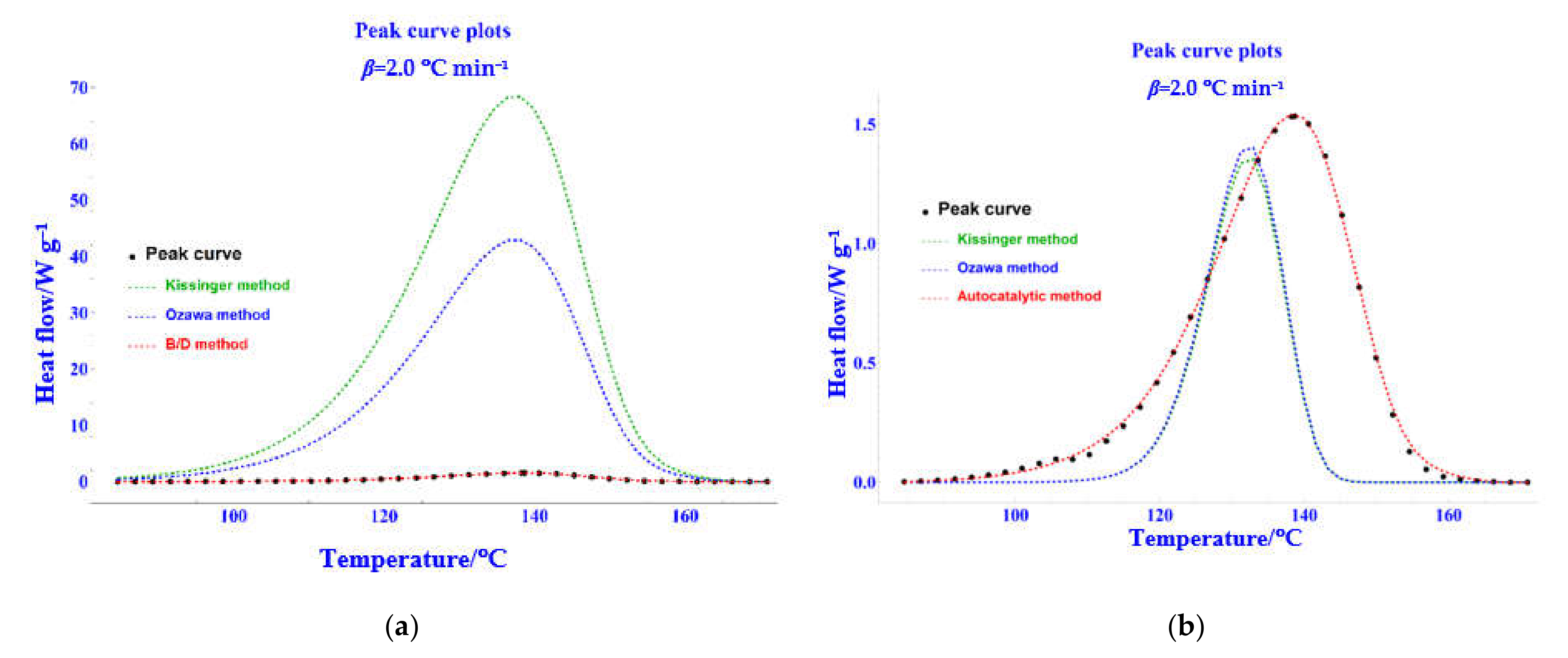
3.2.1. Derived Kinetics Parameters of nth Order by B/D Method (ASTM E2041)

The view of the kinetic model is concerned with the degree of conversion. Referring to Figure 4a, the α versus T, the α versus t, and the conversion rate (dα/dt) versus α are plotted on Figure 9a–c.

The kinetic method of Borchardt and Daniels is based on establishing a specified kinetic model f(α) = (1 − α)ⁿ [22] for each DSC measurement. Figure 10a illustrates Arrhenius plots. Derived kinetic parameters are shown in

Table 4. Kinetic parameters of B/D method simulation result of BTBPC.

β/°C min−1	Mass/mg	lnA	Ea/kJ mol−1	n	R2	Mean Error	Stand Derivation
0.5	4.5	33.572	134.431	1	0.9996	0.001	0.010
1	4.6	36.276	143.402	1	0.9999	0.008	0.009
2	5.2	37.122	146.515	1	0.9997	0.011	0.019
4	5.0	37.066	146.780	1	0.9999	0.018	0.034
6	4.8	43.202	168.464	1.15	0.9998	0.006	0.036
8	4.6	42.491	166.832	1.16	0.9995	0.021	0.063
10	4.6	44.292	173.542	1.21	0.9989	0.058	0.149

. The simulation plots by nth order kinetic parameters are shown in Figure 10b.

3.2.2. Isothermal and Isoconversional Simulation

From the results of B/D test, isothermal predictive curves can be simulated by the rate constant at given temperature near T₀ and between T₀ and T_p, solving the g(α) to acquire the corresponding conversion rate (α) (Equation (13)). The DSC measurement of β = 0.5 was used for simulation where g(α) = −ln(1 − α) (Figure 11a). The isoconversional curves were calculated by fitting with the specific temperature T at given conversion fraction (α), and k(T) yielded the corresponding reaction time (Figure 11b).

3.3. Ozawa Analysis Method (ASTM E698)

The ASTM E698 method was employed to derive values for the kinetic parameters E_a, A, and n by at least four heating rates (β = 0.5, 1, 2, and 4 °C min⁻¹) with peak curve data under the assumption of a first-order reaction. We used two peak temperatures, T_P and T_P-ext, for calculation, respectively; the test results of E_a were 125.53 and 127.23 kJ mol⁻¹, the test results of lnA were 34.90 and 34.78, and the corresponding R² values were 0.9993 and 0.9986, respectively.

Table 5. Relevant parameters for BTBPC simulation analysis tests using the Ozawa method.

β/°C min−1	n	log10β	Tp/K	TP-ext/K	1/TP	TP-ext−1/K−1	(log10β TP−1)2	(log10β TP-ext−1)2
0.5	1	−0.301	397.99	399.52	0.00251	0.00250	−0.0000019	−0.0000019
1	1	0.000	404.92	406.14	0.00247	0.00246
2	1	0.301	411.84	413.08	0.00243	0.00242	0.0000018	0.0000018
4	1	0.602	419.99	421.34	0.00238	0.00237	0.0000034	0.0000034

presents relevant information obtained using the ASTM E698 method, the resulting curves for which are depicted in Figure 12a,b.

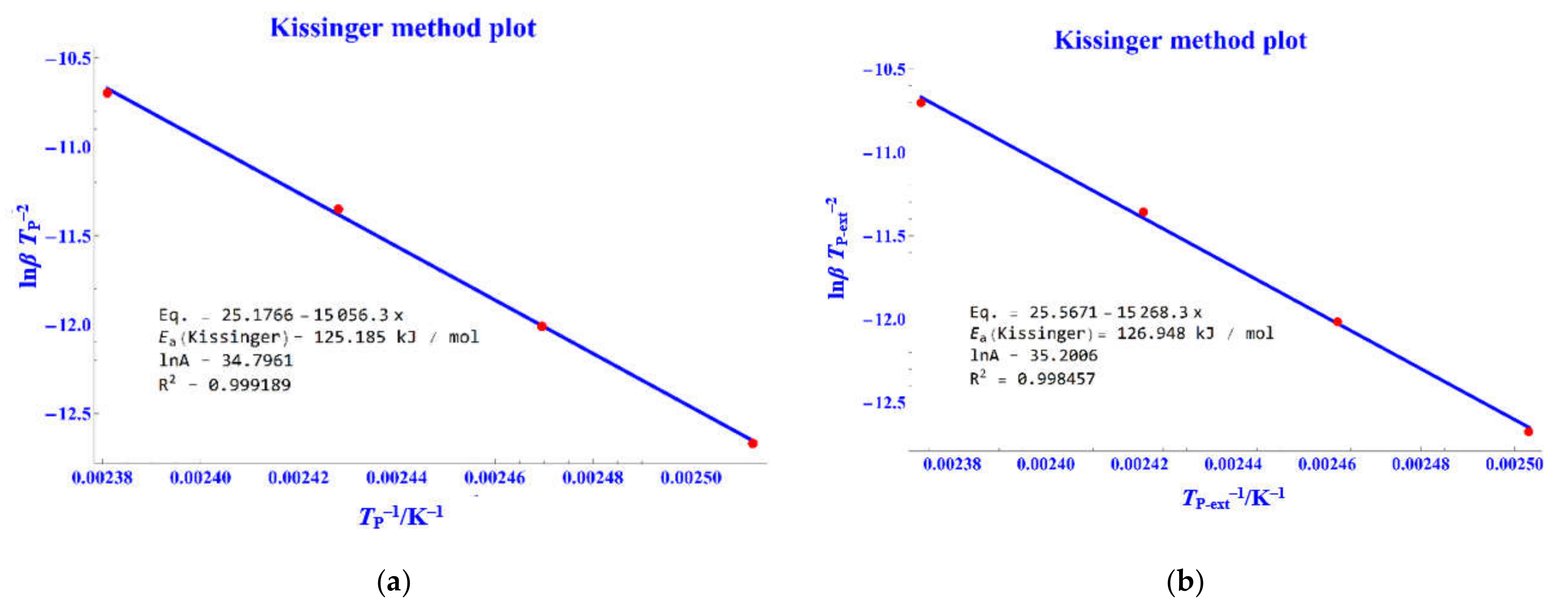
3.4. Kissinger Analysis Method (ASTM E2890)

This method was employed to derive values for the kinetic parameters E_a, A, and n using at least four heating rates (β = 0.5, 1, 2, and 4 °C min⁻¹) with peak curve data under the assumption of the reaction order to a unit. We used two peak temperatures, T_P and T_P-ext, for calculation, respectively (

Table 6. Relevant parameters for BTBPC simulation analysis tests using the Kissinger method.

β/°C min−1	lnβ	TP/K	TP-ext/K	ln[β/Tp2]	ln[β/TP-ext2]	Tp−1/K−1	TP-ext−1/K−1
0.5	−0.693	397.99	399.52	−12.666	−12.674	0.00251	0.00250
1	0.000	404.92	406.14	−12.007	−12.013	0.00247	0.00246
2	0.693	411.84	413.08	−11.348	−11.354	0.00243	0.00242
4	1.386	419.99	421.34	−10.694	−10.701	0.00238	0.00237

); the test results of E_a were 125.185 and 126.948 kJ mol⁻¹, the lnA were 34.7961 and 35.2006, and the corresponding R² values were 0.9992 and 0.9984, respectively. Table 6 presents relevant information obtained using the ASTM E2890 method, and the resulting curves are depicted in Figure 13a,b.

3.5. Derived Autocatalytic Model Parameters

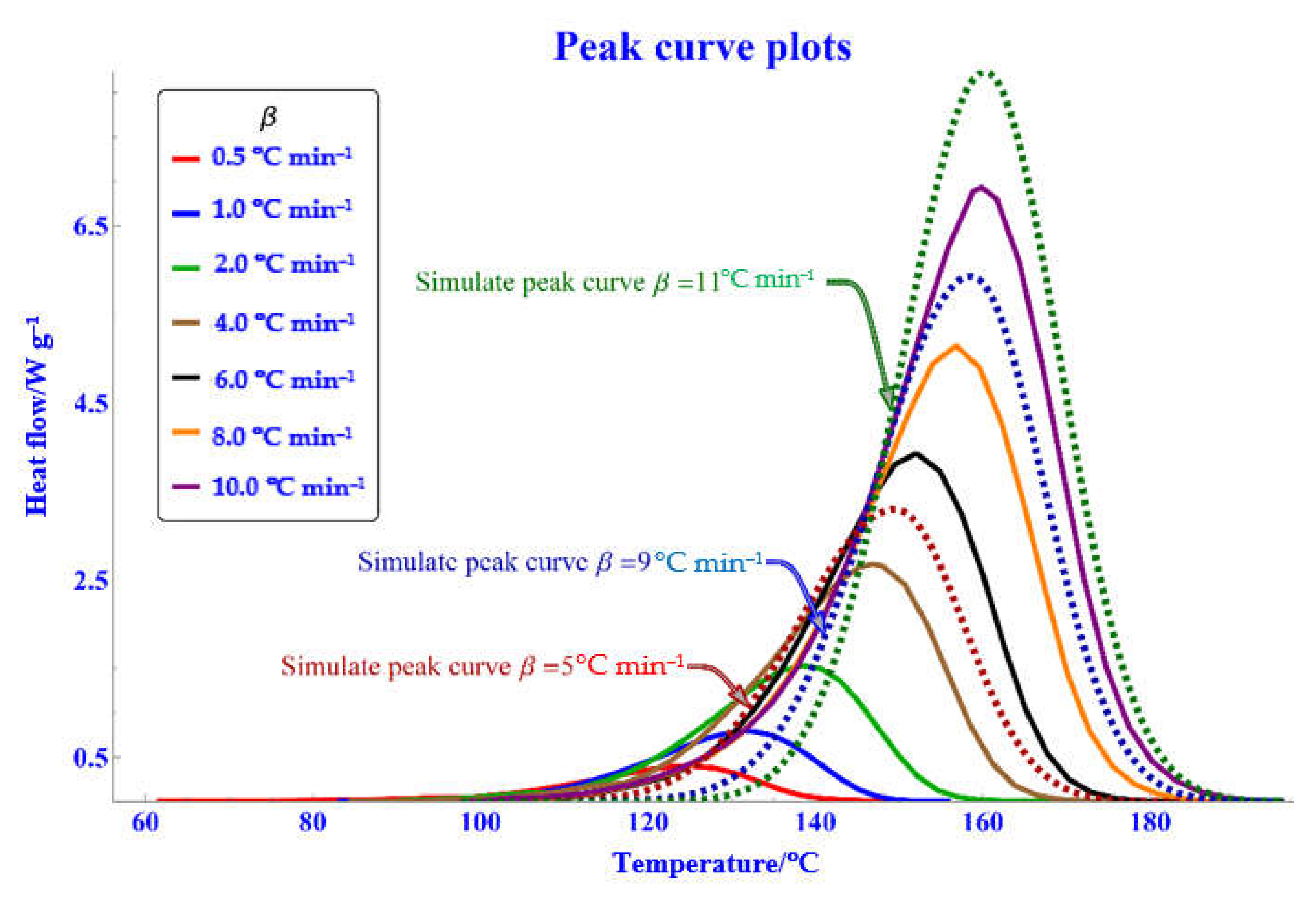
An nth-order reaction rate is dependent only on its reactant concentration(1 − α); an autocatalytic reaction rate is dependent both on its reactant concentration(1 − α), and the product concentration (α) establishes a specified kinetic model f(α) = α^m(1 − α)ⁿ on individual DSC data.

Table 7. Kinetic parameters of B/D method simulation result of BTBPC.

β/°C min−1	Mass/mg	lnA	Ea/kJ mol−1	n	m	R2	Mean Error	Stand Derivation
0.5	4.5	29.369	120.262	1	0.15	0.9997	0.000	0.008
1	4.6	29.206	119.592	0.93	0.15	0.9999	0.006	0.007
2	5.2	32.414	130.103	1	0.15	0.9998	0.005	0.013
4	5.0	32.520	130.622	1	0.15	0.9996	0.007	0.030
6	4.8	36.847	145.890	1.1	0.15	0.9997	−0.004	0.032
8	4.6	36.872	146.606	1.12	0.15	0.9993	0.006	0.065
10	4.6	38.552	152.782	1.16	0.15	0.9989	0.040	0.146

presents the kinetic parameters of the B/D method simulation result, the resulting curves are depicted in Figure 14a,b.

3.6. Prediction

We modeled the peak curves by applying the derived characteristic parameters through the Gaussian curve model, and we also used these to estimate the peak curves for other heating rates. The related parameters for Gaussian simulation were the peak temperature (T_P), the maximum heat flow (q_max), FWHM, and FWHM ratio. These values varied with the heating rate shown in Figure 15.

The three predicted β values (5, 9, and 11 °C min⁻¹) were chosen for simulation of the peak curve of the estimated experiment and plotted as shown in Figure 16. Therefore, these simulation results could be regarded as new DSC measurements from the figure.

4. Discussion

This study was conducted through a model of graphical analysis by way of Mathematica software to derive the associated values of the characteristic parameters and kinetic parameters of the DSC measurements. Compared with the peak curve drawn by combining the derived parameters with the measured values with the original curve, the results are quite consistent.

• Before deriving the characteristic parameters, the raw peak curve of DSC measurement should be normalized first. Drawing a baseline to normalize the peak curve was the first major task and all the characteristics could be derived afterwards.
• We can make simulation predictions through the existing data set for the data of some heating rate that have not been measured yet. The method of these parts could be determined by Section 2.1. and Section 3.6.

There are three major methods for devising the kinetic parameters, described by Section 2.2, Section 2.3 and Section 2.4. The derived kinetics are listed in

Table 8. Derived kinetic parameters comparison.

β	Mass	nth Order Model			Autocatalytic Model				Ozawa Method		Kissinger Method
		lnA	Ea × 103	n	lnA	Ea × 103	n	m	lnA	Ea × 103	lnA	Ea × 103
0.5	4.5	33.572	134.431	1	29.369	120.262	1	0.15	34.934	125.530	34.796	125.185
1	4.6	36.276	143.402	1	29.206	119.592	0.93	0.15
2	5.2	37.122	146.515	1	32.414	130.103	1	0.15
4	5	37.066	146.780	1	32.520	130.622	1	0.15
6	4.8	43.202	168.464	1.15	36.847	145.890	1.1	0.15
8	4.6	42.491	166.832	1.16	36.872	146.606	1.12	0.15
10	4.6	44.292	173.542	1.21	38.552	152.782	1.16	0.15

. The reaction order of all methods was equal to 1, except the β = 1 of the autocatalytic models. The reactions of products of the autocatalytic model were all equal to 0.15. The apparent activation energy of the nth order was higher than the other methods, and the Ozawa and Kissinger methods were close to the autocatalytic model of β = 2. Figure 17 compares nth order versus the Ozawa and Kissinger method plots and the autocatalytic model versus the Ozawa and Kissinger method plots.

• Since identifying autocatalytic reactions is vital in terms of evaluating thermal risks, through the comparison, we could say BTPBC would be ascribed to the class of autocatalytic substances.
• The variation of kinetic parameters, such as the apparent activation energy and the reaction order, would affect the peak curve (Equations (3) and (4) and with reaction model f(α) = (1 − α)ⁿ), as shown in Figure 18. Less reaction would cause peak curve, expansion, and vice versa. Likewise, less apparent activation energy would cause peak curve expansion and vice versa. The above-mentioned is shown in Figure 18a.

5. Conclusions

This study shows that the derived characteristic parameters fit well with the original experimental data. This is because the programs are developed through a general software, and the execution is not limited by equipment and locations. We can spend more time studying various DSC experimental data for those hazardous substances. Since the developed procedures are only sound for simple single-peak DSC measurement, it will be extended to multi-peak data research in the future. We could be sure the method can be used to analyze and verify other different kinds of laboratory data systematically, and it is expected to be able to do more in-depth research on the thermal properties of materials. The procedures can be used to study the parameters for hazardous material in advance and reduce the waste of unnecessary experiments.

References

1. Chen, W.T.; Chen, W.C.; You, M.L.; Tsai, Y.T.; Shu, C.M. Evaluation of thermal decomposition phenomenon for 1,1-bis(tert- butylperoxy)-3,3,5-trimethylcyclohexane by DSC and VSP2. J. Therm. Anal. Calorim. 2015, 122, 1125–1133. [Google Scholar] [CrossRef]
2. Hsueh, K.H.; Chen, W.T.; Chu, Y.C.; Tsai, L.C.; Shu, C.M. Thermal reactive hazards of 1,1-bis(tert-butylperoxy)cyclohexane with nitric acid contaminants by DSC. J. Therm. Anal. Calorim. 2012, 109, 1253–1260. [Google Scholar] [CrossRef]
3. Brown, M.E.; Maciejewski, M.; Vyazovkin, S.; Nomen, R.; Sempere, J.; Burnham, A.; Opfermann, J.; Strey, R.; Anderson, H.L.; Kemmler, A.; et al. Computational aspects of kinetic analysis: Part A: The ICTAC kinetics project-data, methods and results. Thermochim. Acta 2000, 355, 125–143. [Google Scholar] [CrossRef]
4. Ouyang, Q.; Wu, C.; Huang, L. Methodologies, principles and prospects of applying big data in safety science research. Saf. Sci. 2018, 101, 60–71. [Google Scholar] [CrossRef]
5. Pasquetto, I.V.; Borgman, C.L.; Wofford, M.F. Uses and Reuses of Scientific Data: The Data Creators’ Advantage. Harvard Data Sci. Rev. 2019, 12. [Google Scholar] [CrossRef]
6. Pasquetto, I.V.; Randles, B.M.; Borgman, C.L. On the reuse of scientific data. Data Sci. J. 2017, 16, 8. [Google Scholar] [CrossRef] [Green Version]
7. Scalia, G.; Pelucchi, M.; Stagni, A.; Cuoci, A.; Faravelli, T.; Pernici, B. Towards a scientific data framework to support scientific model development. Data Sci. J. 2019, 2, 245–273. [Google Scholar] [CrossRef] [Green Version]
8. Henkelman, G. 100 Trade Center Drive Champaign, IL 61820–7237. Available online: https://www.wolfram.com/mathematica/index.php.en?source=footer (accessed on 5 May 2022).
9. Hsueh, K.H.; Chen, W.C.; Liu, S.H.; Shu, C.M. Thermal parameters study of 1,1-bis(tert-butylperoxy)cyclohexane at low heating rates with differential scanning calorimetry. J. Therm. Anal. Calorim. 2014, 118, 1675–1683. [Google Scholar] [CrossRef]
10. Brown, M.E. Introduction to Thermal Analysis: Techniques and Applications, 2nd ed.; Chapman and Hall: New York, NY, USA, 2001; pp. 181–214. ISBN 978-1-4020-0472-8. [Google Scholar]
11. Chiang, C.L.; Liu, S.H.; Cao, C.R.; Hou, H.Y.; Shu, C.M. Multiapproach thermodynamic and kinetic characterization of the thermal hazards of 2, 2’-azobis (2-methylpropionate) alone and when mixed with several solvents. J. Loss Prev. Process Ind. 2018, 51, 150–158. [Google Scholar] [CrossRef]
12. Gao, P.F.; Liu, S.H.; Zhang, B.; Cao, C.R.; Shu, C.M. Complex thermal analysis and runaway reaction of 2,2’-azobis (isobutyronitrile) using DSC, STA, VSP2, and GC/MS. J. Loss Prev. Process Ind. 2019, 60, 87–95. [Google Scholar] [CrossRef]
13. Wang, S.; Peng, X.; Yang, S.; Li, H.; Zhang, J.; Chen, L.; Chen, W. Numerical and experimental studies on decomposition and vent of di-tertbutyl peroxide in pressure vessel. Process Saf. Environ. Prot. 2018, 120, 97–106. [Google Scholar] [CrossRef]
14. Liu, S.H.; Cao, C.R.; Lin, W.C.; Shu, C.M. Experimental and numerical simulation study of the thermal hazards of four azo compounds. J. Hazard. Mater. 2019, 365, 164–177. [Google Scholar] [CrossRef] [PubMed]
15. TA Instrument. Interpreting Unexpected Events and Transitions in DSC Results. Available online: https://www.tainstruments.com/pdf/literature/TA039.pdf (accessed on 5 May 2022).
16. TA Instrument. A Review of DSC Kinetics Methods. Available online: https://www.tainstruments.com/pdf/literature/TA073.pdf (accessed on 5 May 2022).
17. STARe Software. Available online: https://www.eng.uc.edu/~beaucag/Classes/Characterization/DMA Lab/DMA STARe SW manual ver 9_0 red.pdf (accessed on 5 May 2022).
18. Wolfram Research, Manipulate, Wolfram Language Function. Available online: https://reference.wolfram.com/language/ref/Manipulate.html (accessed on 5 May 2022).
19. Wolfram Research, Using Manipulate to Dynamically Correct the Baseline of a Signal. Available online: https://mathematica.stackexchange.com/questions/58858/using-manipulate-to-dynamically-correct-the-baseline-of-a-signal (accessed on 5 May 2022).
20. Tseng, J.M.; Hsieh, T.F.; Chang, Y.M.; Yang, Y.C.; Chen, L.Y.; Lin, C.P. Kinetic prediction of thermal hazard of liquid organic peroxides by non-isothermal and isothermal kinetic model of DSC tests. J. Therm. Anal. Calorim. 2011, 1093, 1095–1103. [Google Scholar] [CrossRef]
21. Netzsch Group. An Introduction to n-th Order and Autocatalysis Reactions. Available online: https://kinetics.netzsch.com/es/learn/n-th-order-autocatalitic-reactions/ (accessed on 5 May 2022).
22. Mettler-Toledo. Kinetics nth Order-Overview. Available online: https://www.mt.com/sg/en/home/products/Laboratory_Analytics_Browse/TA_Family_Browse/TA_software_browse/STARe_Software_Option_Kinetics_Order_1.html (accessed on 15 December 2021).
23. 23. ASTM E2041; Standard Test Method for Estimating Kinetic Parameters by Differential Scanning Calorimeter Using the Borchardt and Daniels Method. ASTM International: West Conshohocken, PA, USA, 2018.
24. TA Instrument. Reviewing and Comparing of DSC Kinetics Methods. Available online: https://www.azom.com/article.aspx?ArticleID=12105 (accessed on 5 May 2021).
25. Khawam, A.; Flanagan, D.R. Solid-state kinetic models: Basics and mathematical fundamentals. J. Phys. Chem. 2006, 110, 17315–17328. [Google Scholar] [CrossRef]
26. Heinze, S.; Echtermeyer, A.T. A practical approach for data gathering for polymer cure simulations. Appl. Sci. 2018, 8, 2227. [Google Scholar] [CrossRef] [Green Version]
27. Snegirev, A.Y.; Talalov, V.A.; Stepanov, V.V.; Korobeinichev, O.P.; Gerasimov, I.E.; Shmakov, A.G. Autocatalysis in thermal decomposition of polymers. Polym. Degrad. Stab. 2017, 137, 151–161. [Google Scholar] [CrossRef]
28. ASTM E2070; Standard Test Method for Kinetic Parameters by Differential Scanning Calorimetry Using Isothermal Methods. ASTM International: West Conshohocken, PA, USA, 2003.
29. Wolfram Research, LinearModelFit, Wolfram Language Function. Available online: https://reference.wolfram.com/language/ref/LinearModelFit.html (accessed on 5 May 2022).
30. Vyazovkin, S.; Wight, C.A. Model-free and model-fitting approaches to kinetic analysis of isothermal and nonisothermal data. Thermochim. Acta 1999, 340, 53–68. [Google Scholar] [CrossRef]
31. Drozin, D.; Sozykin, S.; Ivanova, N.; Olenchikova, T.; Krupnova, T.; Krupina, N.; Avdin, V. Kinetic calculation: Software tool for determining the kinetic parameters of the thermal decomposition process using the Vyazovkin Method. SoftwareX 2020, 11, 100359. [Google Scholar] [CrossRef]
32. Šimon, P. Isoconversional methods. J. Therm. Anal. Calorim. 2004, 76, 123–132. [Google Scholar] [CrossRef]
33. Flynn, J.H. The isoconversional method for determination of energy of activation at constant heating rates. J. Therm. Anal. Calorim. 1983, 27, 95–102. [Google Scholar] [CrossRef]
34. Stanko, M.; Stommel, M. Kinetic prediction of fast curing polyurethane resins by model-free isoconversional methods. Polymers 2018, 10, 698. [Google Scholar] [CrossRef] [PubMed] [Green Version]
35. Abliz, D.; Artys, T.; Ziegmann, G. Influence of model parameter estimation methods and regression algorithms on curing kinetics and rheological modelling. J. Appl. Polym. Sci. 2017, 134, 45137. [Google Scholar] [CrossRef]
36. Bernath, A.; Kärger, L.; Henning, F. Accurate cure modeling for isothermal processing of fast curing epoxy resins. Polymers 2016, 8, 390. [Google Scholar] [CrossRef]
37. Jansen, K.M.B.; Qian, C.; Ernst, L.J.; Bohm, C.; Kessler, A.; Preu, H.; Stecher, M. Kinetic characterisation of molding compounds. In Proceedings of the 2007 International Conference on Thermal, Mechanical and Multi-Physics Simulation Experiments in Microelectronics and Micro-Systems, EuroSime, London, UK, 16–18 April 2007; pp. 1–5. [Google Scholar]
38. Vafayan, M.; Beheshty, M.H.; Ghoreishy, M.H.R.; Abedini, H. The prediction capability of the kinetic models extracted from isothermal data in non-isothermal conditions for an epoxy prepreg J. Compos. Mater. 2014, 48, 1039–1048. [Google Scholar] [CrossRef]
39. Zhang, C.; Binienda, W.K.; Zeng, L.; Ye, X.; Chen, S. Kinetic study of the novolac resin curing process using model fitting and model-free methods. Thermochim. Acta 2011, 523, 63–69. [Google Scholar] [CrossRef]
40. ASTM E698; Standard Test Method for Kinetic Parameters for Thermally Unstable Materials Using Differential Scanning Calorimetry and the Flynn/Wall/Ozawa Method. ASTM International: West Conshohocken, PA, USA, 2016.
41. Blaine, R.L. Interlaboratory Kinetics Studies Using ASTM International Standards E2041 and E698 and Trityl Azide1. Available online: http://www.tainstruments.com/pdf/literature/TA313.pdf (accessed on 5 May 2021).
42. ASTM E 2890; Standard Test Method for Kinetic Parameters for Thermally Unstable Materials by Differential Scanning Calorimetry Using the Kissinger Method. ASTM International: West Conshohocken, PA, USA, 2012.
43. Scientific Events. Predicting DSC Measurements-STK-Online Scientific events. Available online: http://www.stk-online.ch/Sisseln 2011/Compil_Baati Nadia.pdf (accessed on 5 May 2022).
Figure 1. DSC data structure and data cleansing for BTBPC.
Processes 10 01026 g001
Figure 2. The procedure of DSC characteristic parameters derivation. (a) Peak curve recovery; (b) peak curve normalization; (c) characteristic temperature calculation; (d) total heat of decomposition (ΔHd) calculation.
Processes 10 01026 g002
Figure 3. Gaussian curve simulation method. (a) Gaussian curve’s simulation parameters; (b) Gaussian curve simulation.
Processes 10 01026 g003
Figure 4. Procedures of B/D method. (a) Schematic diagram of related characteristic parameters; (b) calculated {T, α} record with equally spaced values between the temperature limits determined.
Processes 10 01026 g004
Figure 5. The Arrhenius plot showed the left side was derived by the B/D method, the right side was the real-time dynamic simulation curve which the curve was plotted by fitting the derived kinetic parameters into the DSC measurement records {T, α}.
Processes 10 01026 g005
Figure 6. The Arrhenius plot showed on the left side was derived by the autocatalytic model method, the right side was the real-time dynamic simulation curve which the curve was plotted by fit-ting the derived kinetic parameters into the DSC measurement records {T, α}.
Processes 10 01026 g006
Figure 7. Peak curve plot (a) peak curve of the original DSC data (heat flow versus temperature); (b) normalized peak curve (heat flow versus temperature), (c) normalized peak curve (heat flow versus time).
Processes 10 01026 g007
Figure 8. Gaussian simulation curve and DSC measurement curve comparison plots.
Processes 10 01026 g008
Figure 9. The degree of conversion-related plots (a) α versus T plots; (b) α versus t plots; (c) (dα/dt) versus α plots.
Processes 10 01026 g009
Figure 10. B/D method (ASTM E2041) plots (a) Arrhenius plots; (b) simulation curves by nth order kinetic parameters.
Processes 10 01026 g010
Figure 11. Application of rate constant k(T): (a) isothermal simulation result plots; (b) iso-conversional simulation result plots.
Processes 10 01026 g011
Figure 12. ASTM E698 method plot (a) log β versus 1/Tp plot; (b) log β versus 1/TP-ext plot.
Processes 10 01026 g012
Figure 13. ASTM E2890 method plot (a) lnβ/TP2 versus 1/TP plot; (b) lnβ/TP2 versus 1/TP-ext plot.
Processes 10 01026 g013
Figure 14. Autocatalytic model method (a) Arrhenius plots; (b) simulation curves by autocatalytic model kinetic parameters.
Processes 10 01026 g014
Figure 15. Plots of the characteristic temperatures and heat flux versus various of β.
Processes 10 01026 g015
Figure 16. Forecast on different β of Gaussian curve simulation result.
Processes 10 01026 g016
Figure 17. Comparison of nth kinetic model results. (a) nth-order versus the Ozawa and Kissinger method plots; (b) autocatalytic model versus the Ozawa and Kissinger method plots.
Processes 10 01026 g017
Figure 18. Effects of varying nth kinetic parameter (a) variation on reaction order; (b) variation on apparent activation energy.
Processes 10 01026 g018