Machine-Learning-Assisted Prediction of Maximum Metal Recovery from Spent Zinc–Manganese Batteries

Abstract

Spent zinc–manganese batteries contain heavy toxic metals that pose a serious threat to the environment. Recovering these metals is vital not only for industrial use but also for saving the environment. Recycling metal from spent batteries is a complex task. In this study, machine-learning-based predictive models are developed for predicting metal recovery from spent zinc–manganese batteries by studying the energy substrates concentration, pH control of bioleaching media, incubating temperature and pulp density. The main objective of this study is to make a detailed comparison among five machine learning models, namely, linear regression, random forest regression, AdaBoost regression, gradient boosting regression and XG boost regression. All the machine learning models are tuned for optimal hyperparameters. The results from each of the machine learning models are compared using several statistical metrics such as $R^2$, mean squared error (MSE), mean absolute error (MAE), maximum error and median error. The XG Boost regression model is observed to be the most effective among the tested algorithms.

1. Introduction

Batteries have become an indispensable part of our lives and are being increasingly used for many newer applications. The applications range from household battery use to electric vehicles. They are used in electronic compact devices such as electric toys, watches, and remote controls among other devices [1]. The batteries used in the various applications have a given lifetime implying that the volume of used batteries over the past years is on the rise and creative recycling processes are necessary. As there is an increase in the use of EVs, the volume of batteries reaching their end of life is increasing proportionally and it is estimated to dramatically rise in the next five to ten years [2].

Environmental concerns and energy requirements have made the market for electric vehicles expand and become popular in the recent decade. Battery packs are the energy supply units for EVs. The battery packs that are used are made up of Li-ion, Zn–Mn or Ni–Cd [3]. The battery packs typically consist of multiple cells connected in series or parallel. The wide use of lithium-ion batteries (LIBs) in EV power systems is attributed to their long service life, high power/energy density as well as their low rate of discharge [2]. In 2019, the EV annual sales were USD 2.2 million and it is predicted that by 2025, sales of EV LIBs will be more than USD 30 billion [4]. Lithium-ion battery packs are required to be used in EVs for approximately eight to ten years after which they need to be replaced when they attain a capacity loss of 20% [3]. The yearly weight of LIBs that have been retired across the globe is more than 0.5 million tons as of 2020 and it is estimated that a total of 6.8 million units of retired EV packs will be reached by 2035 [4].

In the household battery economy, primary batteries and secondary batteries are used. The primary batteries are those that are not rechargeable. Various types of primary batteries exist such as alkaline zinc–manganese and the most common one is the zinc–carbon battery [5]. Secondary batteries on the other hand are rechargeable. Some of the secondary batteries are lithium-ion (Li-ion), nickel–cadmium (Ni-Cd), nickel–zinc (Ni-Zn), lead–acid, and nickel–metal hydride (NiMH) batteries. The logistics and feasibility of recycling household batteries are affected by the battery recycling technologies available for different battery systems as well as the recycling costs [6]. In household batteries, the metals of concern are manganese, zinc, nickel, cadmium and mercury. There is a possibility of one or more of the metals outlined to be released into the environment; thus, there is a need for a robust technic for maximum metal recovery during the battery recycling process [7].

The traditional ways of dealing with spent LIBs include disposal, reuse and recycling. Disposal implies discarding the retired lithium-ion batteries and is not an environmentally friendly approach as it results in the release of toxic elements, such as nickel and cobalt into the environment, that in turn would adversely impact human health and influence the quality of the environment [8]. The recycling approach of retired LIBs is of critical importance to sustainable development. Through the recycling process, retired batteries can be separated into various components and extraction of valuable materials done [9]. The reuse approach implies that qualified lithium-ion batteries may be re-used in other applications if they pass the assessment criteria for reuse. To address the environmental and economic concerns, it is more suitable to prioritize recycling and reuse approaches rather than the disposal of retired LIBs [10]. Recycling spent batteries is environmentally beneficial in reducing disposal and material recovery for reuse [3]. Legislations on battery waste are increasingly being enforced, for instance, the one implemented in California, Canada, and Europe [11].

Management of the end of life of batteries must be done carefully. The retired batteries have several valuable resources such as zinc, manganese, lithium, aluminium, nickel and cobalt that can be recycled to minimize the resource requirement [10]. Cobalt, for instance, is a less common type of metal and hence recovering it is essential and profitable [8]. Environmental protection is the other argument for recycling batteries. Recycling helps to avoid pollution by preventing toxic materials and heavy metals contained in batteries from entering the waste stream. Recycling batteries is crucial for sustainable development. It helps to recover valuable resources into the value chain [12]. The valuable resources include cathode active elements and metals. Therefore, the proper extraction of these valuable resources (metals) from spent batteries is essential.

The recovery of zinc and manganese is very necessary for the treatment of waste in spent zinc–manganese batteries. Spent zinc–manganese forms a major volume of the overall spent batteries due to their use in household applications [13]. The composition of zinc and manganese is approximately between 14% and 29% for zinc and between 27% and 44% for manganese [14]. There are several available commercial processes such as hydrometallurgy and pyrometallurgy for recycling these types of batteries. Such type of process is quite energy-intensive and poses risky working conditions related to the processes [5,11].

The recovery of valuable metals such as lithium, zinc, nickel, cobalt, manganese, and cadmium from spent batteries is important in addressing environmental concerns. Zinc and manganese are some of the metals with a high percentage of composition in zinc manganese batteries (ZMB) because of their low cost, thus making the ZMB to be widely used and due to their short life, they occupy a large proportion of spent batteries [15]. In terms of the percentage of composition in spent batteries, zinc (Zn) has between 12% and 28% while manganese (Mn) has between 26% and 45% [14]. The existing commercially used metal recovery processes such as hydrometallurgy and pyrometallurgy are heavily polluting, energy-intensive and are associated with high risk [16]. The bio-leaching process, on the other hand, though it is environmentally friendly and not energy-intensive, cannot be commercially used until it is proved that its cost of use is less compared to hydrometallurgy and pyrometallurgy processes [17].

Very recently, several studies have been conducted to assess the impact of using machine learning and artificial intelligence in assisting in various facets of spent battery management. Garg et al. [18] used self-organizing map neural networks to screen and classify spent lithium batteries. They showed that the capacity of reuse battery packs can be improved by 25% by selecting the batteries using self-organizing maps neural networks instead of random selection. Ng et al. [19] used machine learning algorithms to accurately and quickly predict the state of a battery. Lu et al. [20] developed an automatic disassembly system for spent batteries using machine learning algorithms. They relied on computer vision to classify the batteries. Liu et al. [21] used a Gaussian process regression algorithm to predict the life of a lithium-ion battery. Ruhatiya et al. [22] used a polynomial regression model to determine the amount of metal that can be recovered from spent batteries.

Besides battery management, there are several other fields where machine learning prediction models are providing to be very useful. Bhattacharya et al. [23] analyzed the prediction performance of various regression models in composite material property predictions. Shanmugasundar et al. [24] compared AdaBoost and random forest regression in non-traditional machining applications. Jain et al. [25] used random forest regression for predicting the flow characteristics in curved pipes. Kalita et al. [26] studied the utility of various basis functions of radial basis function networks in the prediction of frequency parameters of composites.

The prime objective of the paper is to evaluate the performance of five supervised machine learning models employed in developing prediction models for zinc and manganese recovery from used batteries. An elaborate evaluation of linear regression, random forest regression, AdaBoost regression, gradient boosting regression and XG Boosting regression is carried out for spent zinc–manganese batteries. The objective is to compare the outcomes and establish a machine learning model that contributes the best to the optimal metal recovery of Zn and Mn from spent batteries. A description of each model and what can be discovered, learnt and forecasted with each of the models is presented and the performance of each model is compared by using an array of accuracy metrics such as $R^2$, mean squared error (MSE), mean absolute error (MAE), maximum error and median error. These five machine learning algorithms are chosen due to their popularity among researchers and practitioners. The outcome of this study will provide some definitive answers regarding which is the most suitable machine learning algorithm to be used for such critical problems.

2. Methods

2.1. Linear Regression

Linear regression is a commonly used approach in statistics and machine learning. Linear regression is a supervised model that seeks to find the best linear relationship between the independent variable and the dependent variable. Linear regression encompasses locating statistically significant relationships between two or more variables [27]. The main aim of a linear regression model is to find the best-fit linear line and the optimal values of coefficients and intercepts such that the error is reduced. The difference between the forecasted value and the actual is what is referred to here as an error and the objective is to minimize this difference [28]. The linear regression model has two key goals: establishing a positive relationship between two variables in case the two variables move together, and establishing a negative relation in case there is an increase in one variable that causes a decline in the other variable. In essence, there are two components (i.e., the dependent variable and the independent variable) in linear regression and the two components have different functions. The independent variable explains the significance of factors influencing the model. It is depicted by $x$. The variable that is to be predicted is the dependent variable. It is denoted by $y$. A typical equation for the linear regression is given by:

$$y=mx+c$$

(1)

here $m$ is the gradient and $c$ is the y-intercept.

Statistically, the equation of simple linear regression is written as

$$y=b_0+b_{1}x$$

(2)

In Equation (2), $b_0$ is the $y$ intercept and $b_1$ is the slope or coefficient, $y$ is the dependent variable and $x$ is the independent variable.

For multiple linear regression, i.e., a linear regression having n number of predictors present, then the general equation is given as

$$y=b_0+b_1{x}_1+b_2{x}_2+b_3{x}_3+\cdots +b_n{x}_n$$

(3)

where $y$ is the dependent variable, $b_0$ is the y-intercept, $b_1$, $b_2$… $b_n$ are the slopes or coefficients of the independent variables $x_1$, $x_2$, $x_3$ …. $x_n$.

2.2. Random Forest Regression

Random forest regression is a supervised machine learning algorithm that employs the model ensemble technique for regression. A model ensemble method is an approach that combines prediction from several machine learning algorithms to create a prediction that is more accurate than from a single model. The approach involves training several decision trees where the output of the random forest is given by the average of each of the trained prediction trees [29]. The training time in the random forest is less and the accuracy is high. Random forest regression improves test accuracy and at the same time reduces the costs related to training, storing and fetching inferences from multiple models. In random forest regression, multiple trees are made from a parallel dataset and each tree is independent of one other. A random forest regression model is robust and accurate.

$$RFR prediction=\frac{1}{4}{\displaystyle \sum }_{k=1}^K{h}_k\left(x\right)$$

(4)

where $K$ represents the number of independent regression trees made with input vector $x$. Mean prediction created by $K$ regression trees is represented by $h_k\left(x\right)$.

To compute the mean squared error of the out-of-bag data, the following equation is used

$$MS{E}_{OOB}=\frac{1}{n}{\displaystyle \sum }_{i=i}^n{\left(y_i-\overline{y_{iOOB}}\right)}^2$$

(5)

here, $y_i$ is the $i$^th prediction and $\left(\overline{y_{iOOB}}\right)$ is the average of $i$^th prediction.

Random forest works in a training set (labelled dataset) to make forecasts and generate a model. This approach integrates the concept of bagging with the random choosing of parameters to construct decision trees having controlled variance. A significant benefit of random forest regression as a model is that it may be utilized in establishing variable importance in classification or regression intuitively.

2.3. AdaBoost Regression

AdaBoost Regression is a machine learning sequential ensemble approach. It is a powerful technique whose ensembling power enables the building of a powerful ensemble model even in cases when individual models in the ensemble are extremely simple. This is because AdaBoost assists in combining multiple weak classifiers into one stronger classifier. Machine learning is applied to form weak classifiers. In AdaBoost, the weak learners can be something as simple as a decision tree having a single split, known as decision stumps. The technique functions by assigning more weight to instances that are ‘difficult to classify’ and little weight to instances that have been properly handled. Assigning of weight is done during dataset training and the weights are used in learning every hypothesis. A false prediction is located and assigned further to the next base classifier having low weight and the process is repeated until the output is properly classified by the algorithm [30]. The output, in regression, is not regarded as incorrect; however, it has some absolute value error which might be an arbitrary constant.

2.4. Gradient Boosting Regression

Gradient boosting regression is a popular machine learning algorithm used for tabular datasets. It is robust enough to the extent that it can be utilized in finding any non-linear association between the target model and features and as well as wide usability which may deal with outliers, and missing values without the need of having any distinct treatment. Gradient boosting encompasses three elements which include: a weaker classifier to make predictions, a loss of function to be optimized, and an additive model to assign weak learners to reduce the loss function. The loss function to be used is dependent on the form of the problem that is to be solved. It ought to be differentiable; however, most standard loss functions are underpinned and one can define their own. In gradient boosting, decision trees are used as weak learners. Regression trees that output real values for splits are used and whose output could be combined enabling subsequent model outputs to be added and corrections made in the resulting predictions. The construction of trees is based on a greedy manner and selecting the most suitable split points based on purity scores such as Gini. Weak learners should be constrained in certain ways such as the maximum number of nodes, leaf nodes, layers or splits to make sure that the learners remain weak yet can be constructed greedily. In the additive model, the addition of trees is performed one at a time and those trees already existing in the model remain unchanged. To reduce the loss when trees are added, a gradient descent approach is utilized. Gradient descent minimizes set parameters such as weights in a neural network or coefficients in a regression equation. Once error loss has been calculated, updating the weights is done to reduce that error.

2.5. XG Boost Regression

XG Boost is a supervised machine learning algorithm that attempts to accurately predict a target variable by combining the estimates of a set of simpler, weaker models. It is a popular and efficient implementation of the gradient boosted tree algorithm. The XG Boost has a variety of algorithms that normally come along with their synchronized set of hyperparameters. This makes the model able to add several different trees together. XG Boost reduces a regularized objective role which adds a convex loss function (that is based on the difference between target output and forecasted output) and regression tree functions. Training continues iteratively, that is, by combining new trees which forecast the errors or residuals of preceding trees which are then added to the previous trees to create an ultimate forecast. XG Boost can model different regression, classification or rank tasks through the use of linear functions and trees by utilizing various regulation schemes and through adjusting several other parameters of the respective algorithm.

3. Problem Description

While the precise chemical composition differs from one type of battery to another, most of the batteries have heavy metals that are an environmental concern. Improper disposal of the spent batteries can result in heavy metals leaking into the environment causing water and soil pollution thus endangering life. Zinc and manganese are some of the metals that represent the largest percentage of composition in batteries, especially the primary batteries, thus they are of interest in the process of recycling the spent batteries. Several processes have been undertaken in recovering the valuable metals from spent batteries such as the leaching process of sulfuric and hydrochloric acid media.

Data-driven techniques, for instance, predictive models based on artificial intelligence (AI) employed in several engineering domains depict good results. Approaches such as machine learning algorithms have been used in the copper production industry to for example minimize the costs of leaching processes targeting to enhance processes and outcomes. This implies that machine learning models can be a good candidate for maximum recovery of Zn and Mn from spent batteries. It is necessary to provide the right volume of data in terms of processes and results for the machine learning models to function properly. The eventual aim of using the machine learning models in recovering valuable metals from spent batteries is for maximum metal recovery of Zn and Mn, to be gentle on the environment and to save resources. In this work, a comparative analysis of machine learning models in the maximum metal recovery of zinc and manganese from spent batteries is carried out. The work aims to fill the gap and provide an understanding of the recycling of valuable metals from spent batteries based on the knowledge of machine learning. The dataset used in the study is considered by Ruhatiya et al. [22]. Energy substrates concentration (SC(g/L)), pH control of bioleaching media, incubating temperature (T (°C)) and pulp density (PD %) are considered as the input parameters, whereas the Zn concentration and Mn concentration are the output parameters.

4. Results and Discussion

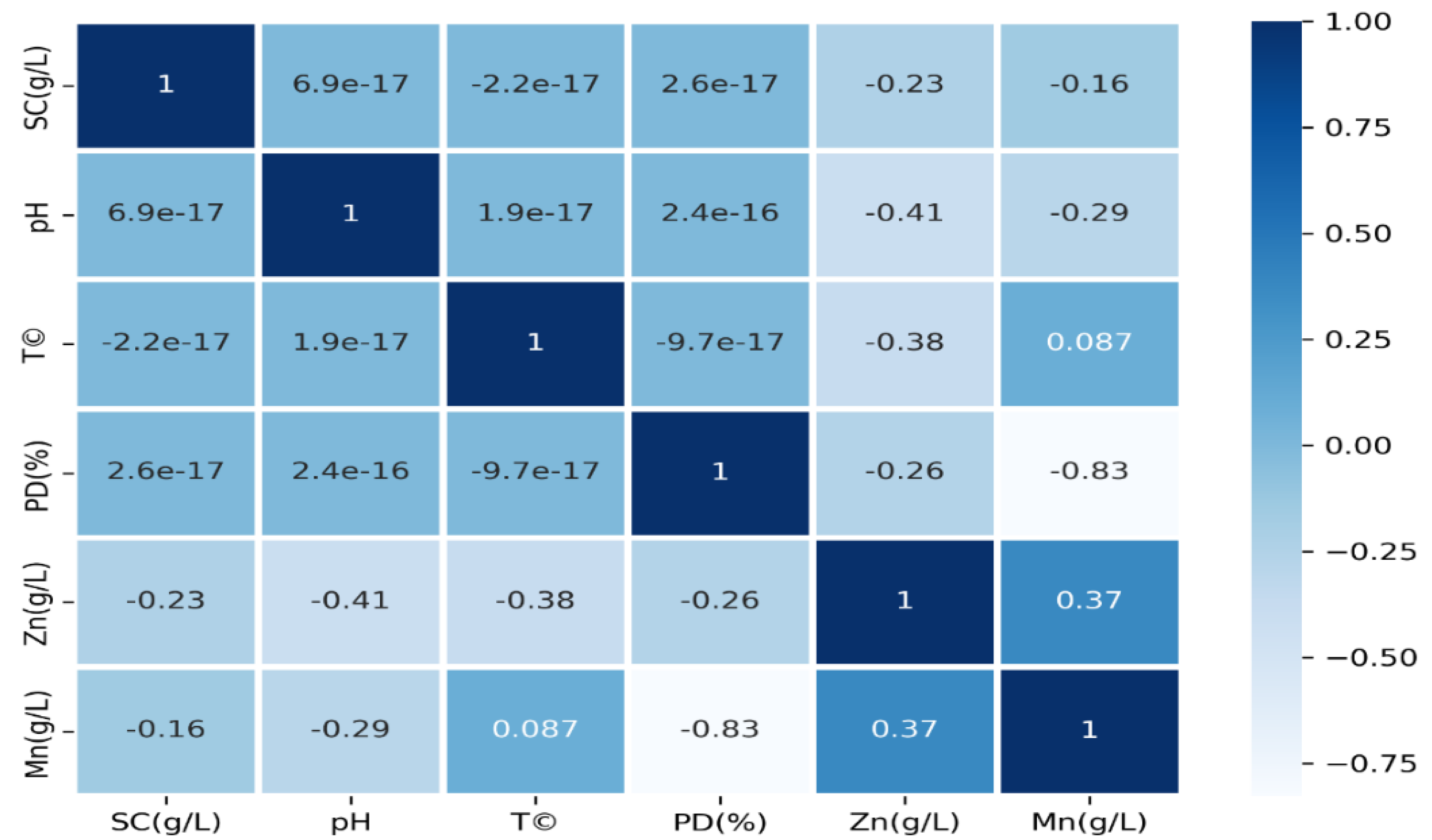
4.1. Data Characteristics

Before the application of machine learning algorithms, it is important to look at the various features of the data that are used to perform statistical analyses to establish trends and patterns in data. The statistical summary of the input parameters and the responses of the dataset are shown in

Table 1. Statistical summary of the dataset.

Statistical Feature	SC (g/L)	pH	T (°C)	PD (%)	Zn (g/L)	Mn (g/L)
Count	29	29	29	29	29	29
Mean	32	2	35	10	7.517	10.417
Standard deviation	3.703	0.185	2.314	0.925	1.794	0.793
Min	24	1.6	30	8	4.6	9.1
25%	28	1.8	32.5	9	6	9.7
50%	32	2	35	10	7.3	10.5
75%	36	2.2	37.5	11	9.1	10.9
Max	40	2.4	40	12	10.3	12.5
Range	16	0.8	10	4	5.7	3.4

. The total dataset sample is 29 that was used in modelling. Data sampling was achieved through a random-sampling algorithm whereby 90% of the data were regarded as a training dataset, while 10% were for testing. It should be noted that typically a 70% to 30% split for training to testing data is considered in ML applications. However, a 90% to 10% split for training to testing data is considered in this paper as the dataset is limited. It is observed that the dataset does not have any missing data.

To further look into the underlying pattern of the data, pair plots for the input parameters and observed responses are depicted in Figure 1. The pair plots are constructed on two key figures, a scatter plot and a histogram. The histogram illustrates the distributions of one variable, whereas the scatter plots depict the relationship between the two variables. From the pair plots, we see that all the input parameters (SC, pH, T and PD) are positively correlated indicating that they influence the maximum recovery of Zn and Mn.

Pearson’s correlation heatmap of input parameters and observed responses is shown in Figure 2. It is seen that there is no significant correlation among the input parameters implying there is no multi-collinearity. T is observed to have a moderately strong negative correlation with Zn and a very low positive correlation with Mn while pH has a moderately strong negative correlation with both Zn and Mn. PD also has a moderately negative correlation with Zn but a very strong correlation with Mn.

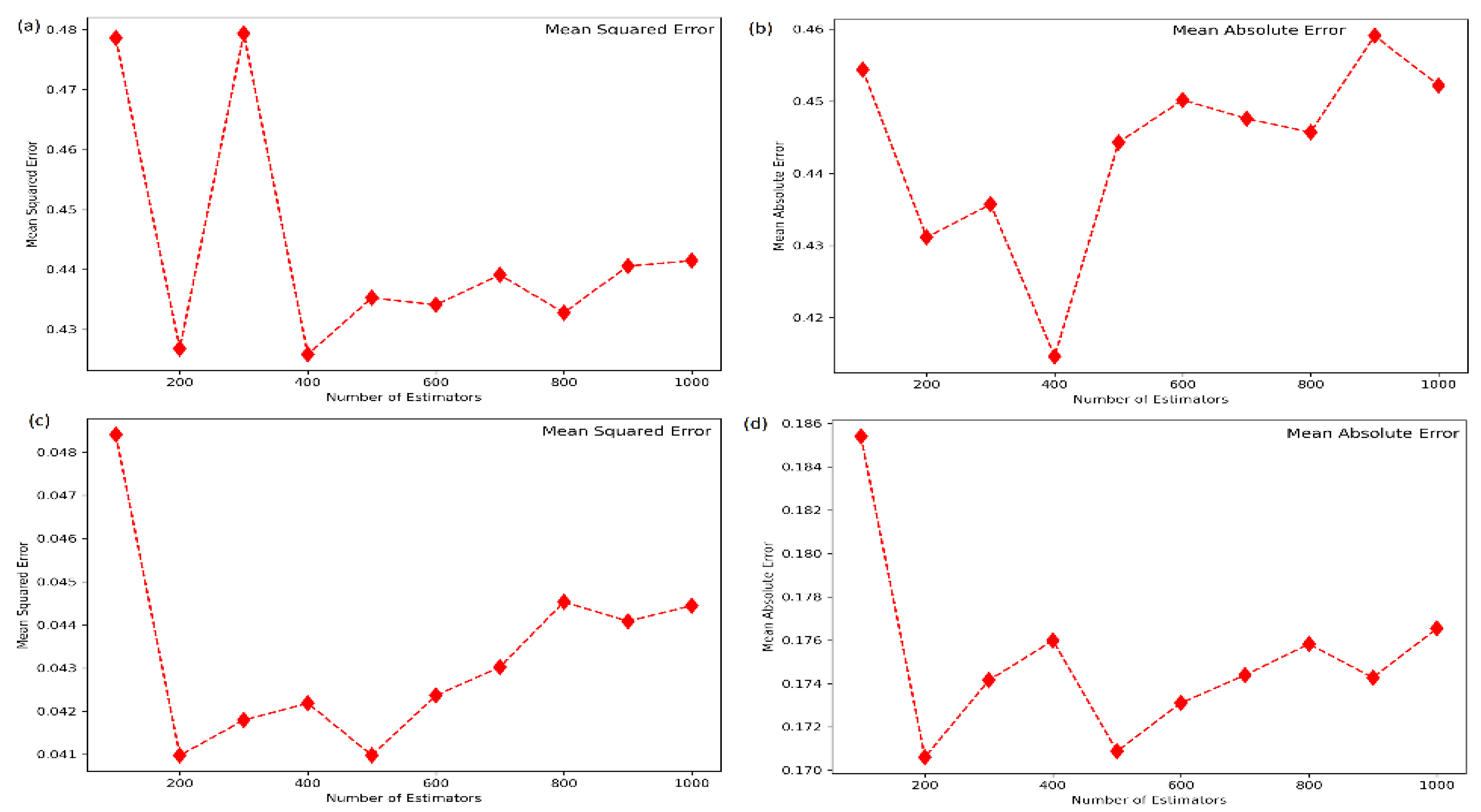
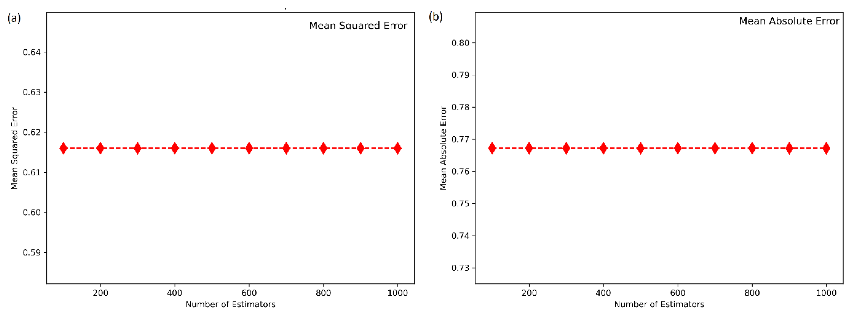
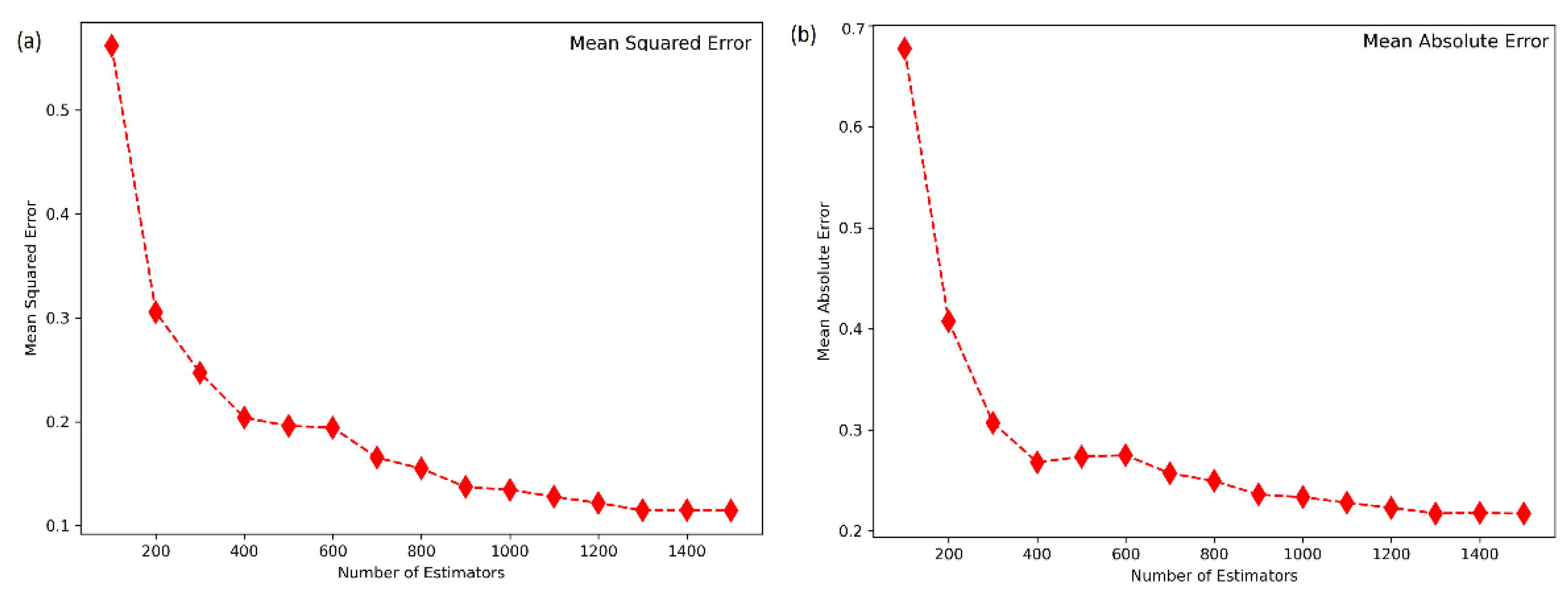
4.2. Hyperparameter Tuning of the Machine Learning Models

It should be noted that the number of estimators is an important hyperparameter for random forest regression; thus, it needs to be tuned. Figure 3 shows the results of the hyperparameter tuning process of the number of estimators random forest regression in terms of MSE and MAE. It is observed that the number of estimators has a huge effect on the MSE and MAE. Nevertheless, 400 and 200 estimators were selected as the optimal while modelling Zn and Mn, respectively.

Similar to the random forest regression, AdaBoost is also tuned for the number of estimators. However, as seen in Figure 4, the AdaBoost is unaffected by the number of estimators. Thus, for the rest of the analysis in this paper, the number of estimators for AdaBoost is considered 100.

The effect of the number of estimators on the gradient boosting regression model is shown in Figure 5 for Zn modelling. An elbow is formed at around 1000 estimators in the gradient boosting regression analysis shown in Figure 5. It is seen that until about 400 estimators there is rapid improvement in the ML model but beyond it the improvement becomes sluggish. A total of 1400 estimators are considered the optimal value for further analysis in this paper. Beyond 1400 estimators, the improvement in the performance characteristics of the increasing number of estimators of the model is very poor.

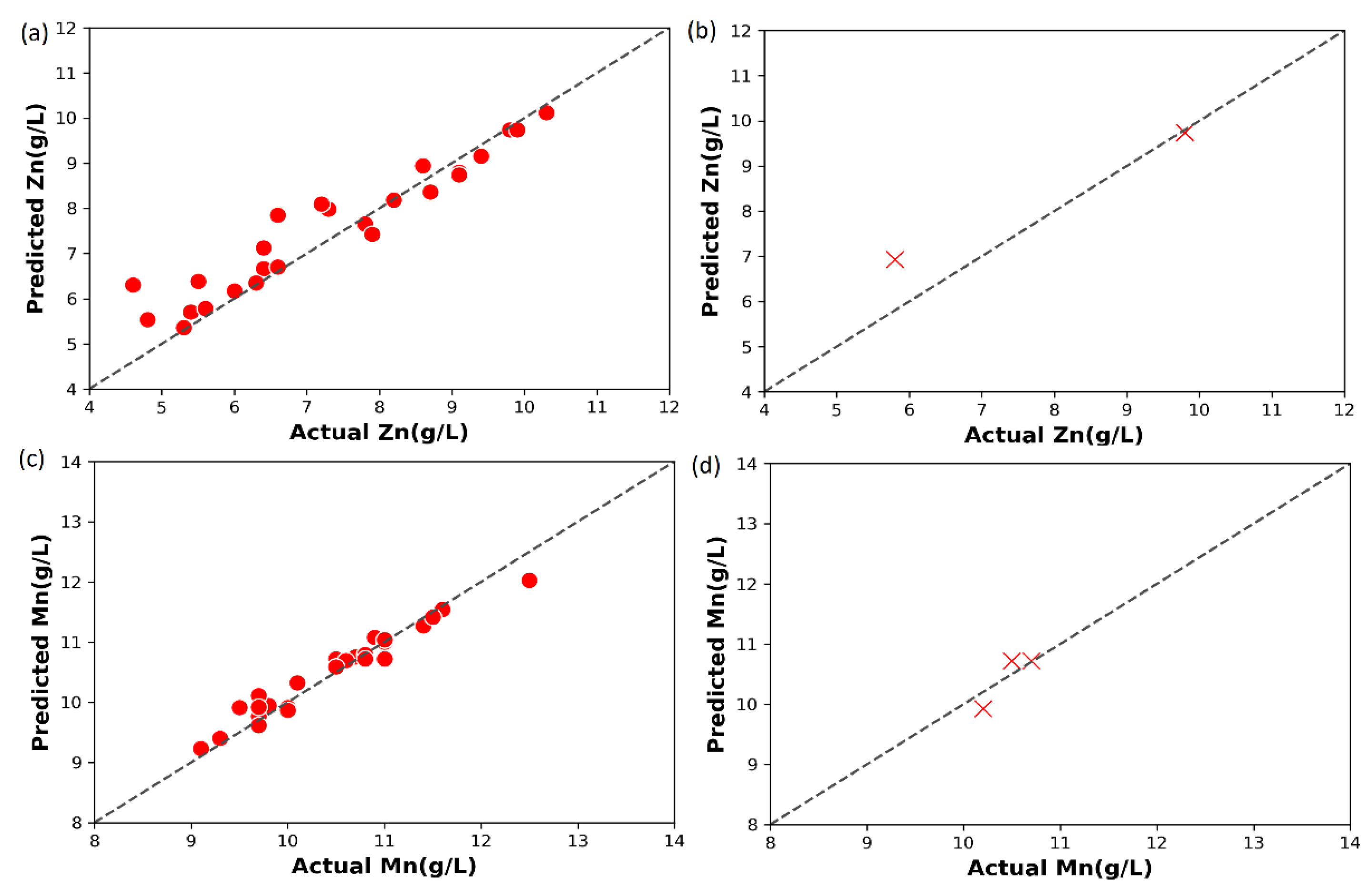
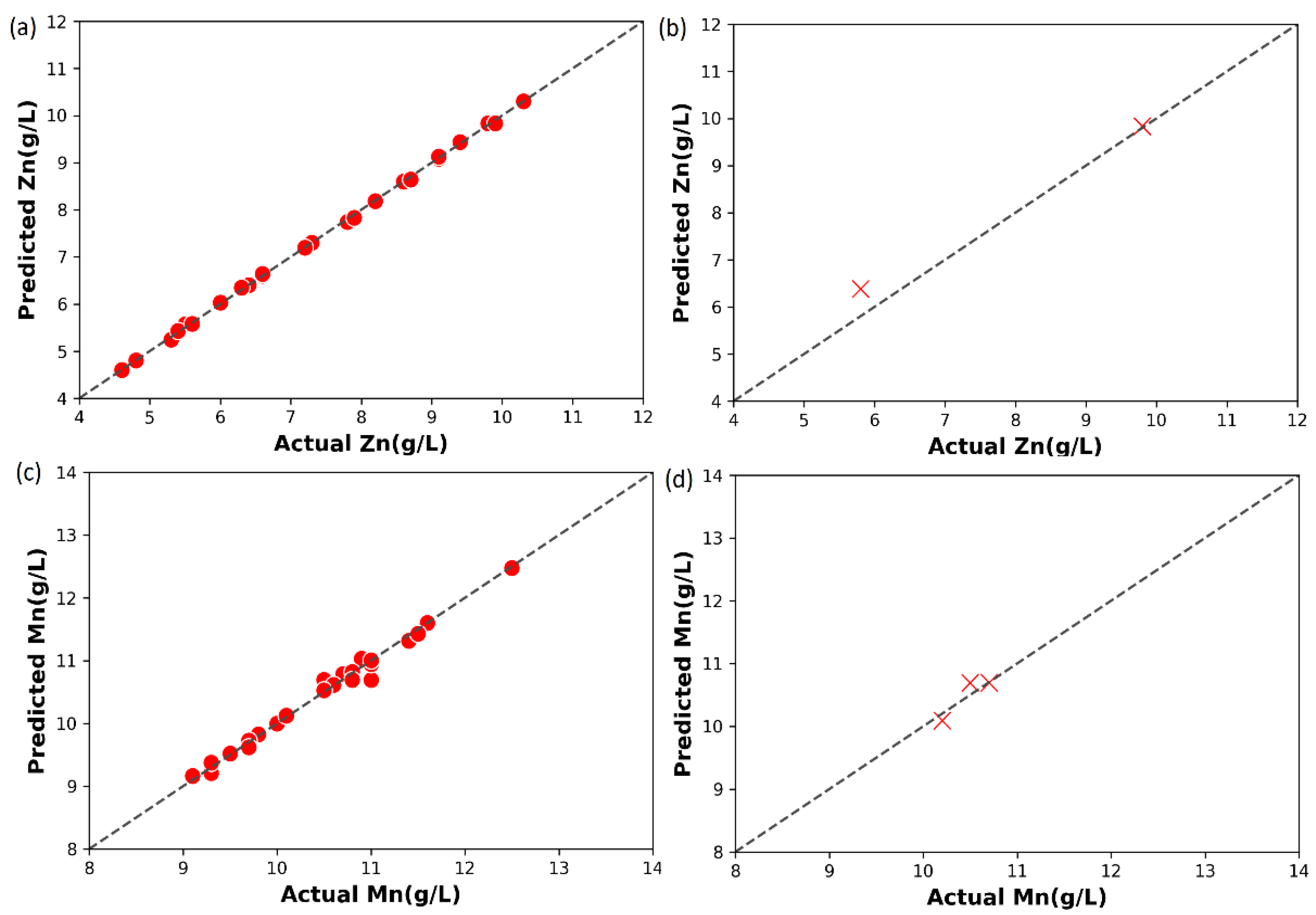
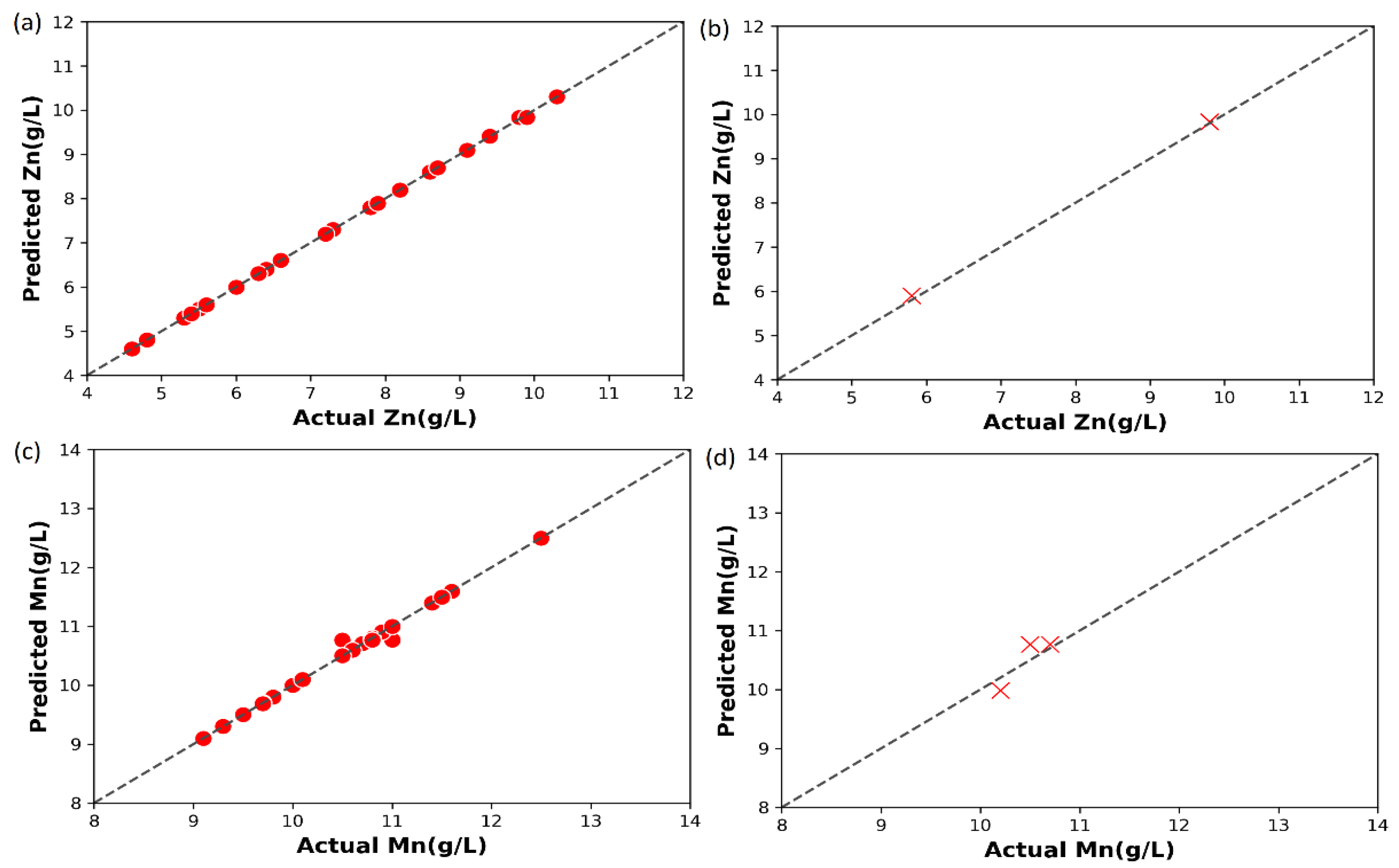
4.3. Performance of the Machine Learning Models

Figure 6 shows the actual versus linear regression-based prediction for Zn and Mn for both training and testing data. For Zn, the predictions are scattered about the diagonal line indicating the presence of deviations. It should be noted that in such predicted versus actual plots, it is desired that predicted data points are as close to the diagonal line as possible. Values below the diagonal indicate underprediction, whereas values above the diagonal indicate overprediction [31,32]. For the linear regression model, the predictions of the Mn model are seen to be better than the Zn model. The reason for this is perhaps the lower standard deviation and range of Mn data as compared to the Zn data. Since the design space spread to be modelled is low for Mn data, the linear regression is able to explain the variance in the data more easily as compared to Zn data.

The prediction performance of the random forest regression machine learning model is shown in Figure 7. It is observed to be better than that of linear regression observed in Figure 6, indicating that some amount of non-linearity in the data was not captured by the linear regression model. Since the random forest is aggregation of many small decision trees, it is able to more accurately estimate the variance in the data. Figure 8 shows the actual versus AdaBoost regression-based predicted observations for training and testing data of both the Zn and Mn models. It is observed that the performance of AdaBoost is poorer than random forest regression but better than the linear regression model. It should be noted that as discussed earlier, even increasing the number of estimators in AdaBoost was not able to improve the prediction quality. The performance of the gradient boosting regression machine learning model is shown in Figure 9. For the training data, the gradient boosting regression model is seen to have a near-ideal estimation. The prediction performance on testing data is very high. Finally, an XG Boost regression machine learning model is used for the Zn and Mn modelling task as shown in Figure 10. The XG Boost regression has excellent prediction capability. There is a very minor deviation in the Mn testing data prediction by the XG Boost regression.

Apart from visually looking at the predictions of any ML model, it is also important to look at them using statistical metrics. To do so and to compare the five machine learning models that are being analyzed, an interaction assessment is performed. This gives some insight into the relationship among the input parameters and the way the output yield is influenced by the input parameters.

Table 2. Performance of the machine learning models on Zn (g/L) data.

Data	Model	${\mathit{R}}^{\mathbf{2}}$	MSE	MAE	Maximum Error	MedAE
Train	Linear Regression	51.88%	1.4157	0.9088	2.4791	0.6072
	Random Forest Regression	88.67%	0.3333	0.4115	1.7072	0.2829
	AdaBoost Regression	85.44%	0.4285	0.5206	1.3500	0.4100
	Gradient Boosting Regression	99.95%	0.0014	0.0279	0.0725	0.0306
	XG Boost Regression	99.99%	0.0003	0.0078	0.0677	0.0019
Test	Linear Regression	−42.33%	5.0605	2.2411	2.3791	2.3791
	Random Forest Regression	88.02%	0.4258	0.4146	1.1273	0.0583
	AdaBoost Regression	82.67%	0.6160	0.7673	0.8842	0.8842
	Gradient Boosting Regression	96.76%	0.1150	0.2177	0.5855	0.0339
	XG Boost Regression	99.88%	0.0041	0.0554	0.1017	0.0323

shows the performance of the machine learning models on Zn and

Table 3. Performance of the machine learning models on Mn (g/L) data.

Data	Model	${\mathit{R}}^{\mathbf{2}}$	MSE	MAE	Maximum Error	MedAE
Train	Linear Regression	80.33%	0.1324	0.2646	0.8467	0.1960
	Random Forest Regression	94.40%	0.0377	0.1513	0.4747	0.1113
	AdaBoost Regression	94.92%	0.0342	0.1476	0.4500	0.1388
	Gradient Boosting Regression	98.78%	0.0082	0.0624	0.3072	0.0285
	XG Boost Regression	99.28%	0.0049	0.0225	0.2651	0.0012
Test	Linear Regression	19.36%	0.0340	0.1517	0.2985	0.0985
	Random Forest Regression	22.96%	0.0410	0.1706	0.2726	0.2196
	AdaBoost Regression	12.32%	0.0559	0.1933	0.3800	0.1400
	Gradient Boosting Regression	61.24%	0.0164	0.1030	0.1928	0.1090
	XG Boost Regression	95.97%	0.0397	0.1805	0.2651	0.2111

shows the performance of the machine learning models on Mn. It is observed that for performance machine learning models on Zn, the highest $R^2$ for both the training dataset and the testing dataset is recorded for XG Boost regression, and the lowest MSE, MAE, maximum error and MedAE both for the training dataset and testing dataset are also recorded for the XG Boost regression model. This implies that XG Boost regression is the most suitable model for optimum recovery of Zn. As compared to the linear regression model, the random forest regression, adaBoost regression, gradient boosting regression and XG boost regression model showed approximately 92%, 88%, 98% and 100% improvement in terms of MSE.

For the performance of the machine learning on Mn, it is observed that the highest $R^2$ and lowest MSE, MAE, maximum error and MedAE are recorded for the XG Boost regression model. It is observed that while modelling Mn, as compared to AdaBoost regression, the other four algorithms, namely linear regression, random forest regression, gradient boosting regression and XG boost regression, showed approximately 57%, 86%, 397% and 678% improvement, respectively, on $R^2$ for testing data.

5. Conclusions

In this paper, five different machine learning models for maximum metal recovery of zinc and manganese were considered. The key objective was to compare the performance of the different machine learning models for maximum metal recovery of zinc and manganese in the recycling process. The input parameters that were considered in the study were SC, PD, T, and pH, whereas the target parameters were the maximum yield of Zn and Mn. The machine learning models that were applied appeared to be efficient methods for ensuring maximum metal recovery of Zn and Mn from spent batteries. They also proved their efficacy in modelling complex interactions between input parameters and responses such as the one in the study. In comparing the efficiency of the different methodologies that were being studied, it was observed that the XG boost regression model is more efficient than the other four models because its maximum margin of error is small (almost negligible) compared to the other methods. From the hyperparameter tuning phase, it was found that AdaBoost is unaffected by the number of estimators used; thus, the need for hyperparameter tuning is less than the other algorithms. This would lead to considerable computational cost savings for the AdaBoost model. However, the gradient boosting regression model is significantly affected by the number of estimators, especially when the number of estimators is low. However, ultimately, the outcome from the global comparison analysis indicated the stability of the different machine learning models used based on the methodology that was applied. Based on both the case studies, the ML algorithms in terms of this study can be ranked from best to worst as XG boost regression, gradient boosting regression, random forest regression, AdaBoost Regression and linear regression.

References

1. Millette Environmental. Research Study on Reuse and Recycling of Batteries Employed in Electric Vehicles: The Technical, Environmental, Economic, Energy and Cost Implications of Reusing and Recycling EV Batteries. Energy API. 2019. Available online: https://www.api.org/~/media/Files/Oil-and-Natural-Gas/Fuels/Kelleher%20Final%20EV%20Battery%20Reuse%20and%20Recycling%20Report%20to%20API%2018Sept2019%20edits%2018Dec2019.pdf (accessed on 5 April 2022).
2. Hua, Y.; Zhou, S.; Huang, Y.; Liu, X.; Ling, H.; Zhou, X.; Zhang, C.; Yang, S. Sustainable value chain of retired lithium-ion batteries for electric vehicles. J. Power Sources 2020, 478, 228753. [Google Scholar] [CrossRef]
3. Eftekhari, A. Lithium Batteries for Electric Vehicles: From Economy to Research Strategy. ACS Sustain. Chem. Eng. 2019, 7, 5602–5613. [Google Scholar] [CrossRef]
4. Chung, D.; Elgqvist, E.; Santhanagopalan, S. Automotive Lithium-ion Cell Manufacturing: Regional Cost Structures and Supply Chain Considerations; National Renewable Energy Lab. (NREL): Golden, CO, USA, 2016. [Google Scholar] [CrossRef] [Green Version]
5. Sayilgan, E.; Kukrer, T.; Civelekoglu, G.; Ferella, F.; Akcil, A.; Veglio, F.; Kitis, M. A review of technologies for the recovery of metals from spent alkaline and zinc–carbon batteries. Hydrometallurgy 2009, 97, 158–166. [Google Scholar] [CrossRef]
6. Reuter, M.; Hudson, C.; Van Schaik, A.; Heiskanen, K.; Meskers, C.; Hagelüken, C. Metal recycling: Opportunities, limits, infrastructure. In A Report of the Working Group on the Global Metal Flows to the International Resource Panel; UNEP: Nairobi, Kenya, 2013. [Google Scholar]
7. Bonhomme, R.; Gasper, P.; Hines, J.; Miralda, J.P. Economic Feasibility of a Novel Alkaline Battery Recycling Process; Worcester Polytechnic Institute: Worcester, MA, USA, 2013. [Google Scholar]
8. Chen, L.; Tang, X.; Zhang, Y.; Li, L.; Zeng, Z.; Zhang, Y. Process for the recovery of cobalt oxalate from spent lithium-ion batteries. Hydrometallurgy 2011, 108, 80–86. [Google Scholar] [CrossRef]
9. Huang, B.; Pan, Z.; Su, X.; An, L. Recycling of lithium-ion batteries: Recent advances and perspectives. J. Power Sources 2018, 399, 274–286. [Google Scholar] [CrossRef]
10. Huang, K.; Li, J.; Xu, Z. Characterization and recycling of cadmium from waste nickel–cadmium batteries. Waste Manag. 2010, 30, 2292–2298. [Google Scholar] [CrossRef]
11. Reuter, M.A.; Kojo, I.V. Challenges of metal recycling. Materia 2012, 2, 50–57. [Google Scholar]
12. Mayyas, A.; Steward, D.; Mann, M. The case for recycling: Overview and challenges in the material supply chain for automotive li-ion batteries. Sustain. Mater.Technol. 2019, 19, e00087. [Google Scholar] [CrossRef]
13. Ruhatiya, C.; Tibrewala, H.; Gao, L.; Sleesongsom, S.; Chin, C.M.M. Intelligent optimization of process conditions for maximum metal recovery from spent zinc-manganese batteries. IOP Conf. Series Earth Environ. Sci. 2020, 463, 012160. [Google Scholar] [CrossRef]
14. Niu, Z.; Huang, Q.; Xin, B.; Qi, C.; Hu, J.; Chen, S.; Li, Y. Optimization of bioleaching conditions for metal removal from spent zinc-manganese batteries using response surface methodology. J. Chem. Technol. Biotechnol. 2014, 91, 608–617. [Google Scholar] [CrossRef]
15. Kim, T.-H.; Senanayake, G.; Kang, J.-P.; Sohn, J.-S.; Rhee, K.-I.; Lee, S.-W.; Shin, S.-M. Reductive acid leaching of spent zinc–carbon batteries and oxidative precipitation of Mn–Zn ferrite nanoparticles. Hydrometallurgy 2009, 96, 154–158. [Google Scholar] [CrossRef]
16. Flores, V.; Leiva, C. A Comparative Study on Supervised Machine Learning Algorithms for Copper Recovery Quality Prediction in a Leaching Process. Sensors 2021, 21, 2119. [Google Scholar] [CrossRef] [PubMed]
17. Ebrahimzade, H.; Khayati, G.R.; Schaffie, M. A novel predictive model for estimation of cobalt leaching from waste Li-ion batteries: Application of genetic programming for design. J. Environ. Chem. Eng. 2018, 6, 3999–4007. [Google Scholar] [CrossRef]
18. Garg, A.; Yun, L.; Gao, L.; Putungan, D.B. Development of recycling strategy for large stacked systems: Experimental and machine learning approach to form reuse battery packs for secondary applications. J. Clean. Prod. 2020, 275, 124152. [Google Scholar] [CrossRef]
19. Ng, M.F.; Zhao, J.; Yan, Q.; Conduit, G.J.; Seh, Z.W. Predicting the state of charge and health of batteries using data-driven machine learning. Nat. Mach. Intell. 2020, 2, 161–170. [Google Scholar] [CrossRef] [Green Version]
20. Lu, Y.; Maftouni, M.; Yang, T.; Zheng, P.; Young, D.; Kong, Z.J.; Li, Z. A novel disassembly process of end-of-life lithium-ion batteries enhanced by online sensing and machine learning techniques. J. Intell. Manuf. 2022, 1–13. [Google Scholar] [CrossRef]
21. Liu, K.; Li, Y.; Hu, X.; Lucu, M.; Widanage, W.D. Gaussian Process Regression With Automatic Relevance Determination Kernel for Calendar Aging Prediction of Lithium-Ion Batteries. IEEE Trans. Ind. Inform. 2019, 16, 3767–3777. [Google Scholar] [CrossRef] [Green Version]
22. Ruhatiya, C.; Shaosen, S.; Wang, C.; Jishnu, A.K.; Bhalerao, Y. Optimization of process conditions for maximum metal recovery from spent zinc-manganese batteries: Illustration of statistical based automated neural network approach. Energy Storage 2019, 2, e111. [Google Scholar] [CrossRef]
23. Bhattacharya, S.; Kalita, K.; Čep, R.; Chakraborty, S. A Comparative Analysis on Prediction Performance of Regression Models during Machining of Composite Materials. Materials 2021, 14, 6689. [Google Scholar] [CrossRef]
24. Shanmugasundar, G.; Vanitha, M.; Čep, R.; Kumar, V.; Kalita, K.; Ramachandran, M. A Comparative Study of Linear, Random Forest and AdaBoost Regressions for Modeling Non-Traditional Machining. Processes 2021, 9, 2015. [Google Scholar] [CrossRef]
25. Jain, P.; Choudhury, A.; Dutta, P.; Kalita, K.; Barsocchi, P. Random Forest Regression-Based Machine Learning Model for Accurate Estimation of Fluid Flow in Curved Pipes. Processes 2021, 9, 2095. [Google Scholar] [CrossRef]
26. Kalita, K.; Chakraborty, S.; Madhu, S.; Ramachandran, M.; Gao, X.-Z. Performance Analysis of Radial Basis Function Metamodels for Predictive Modelling of Laminated Composites. Materials 2021, 14, 3306. [Google Scholar] [CrossRef]
27. Montgomery, D.C.; Peck, E.A.; Vining, G.G. Introduction to Linear Regression Analysis; John Wiley & Sons: Hoboken, NJ, USA, 2021. [Google Scholar]
28. Seber, G.A.; Lee, A. Linear Regression Analysis; John Wiley & Sons: Hoboken, NJ, USA, 2012. [Google Scholar]
29. Li, X. Using “random forest” for classification and regression. Chin. J. Appl. Entomol. 2013, 50, 1190–1197. [Google Scholar]
30. Collins, M.; Schapire, R.E.; Singer, Y. Logistic Regression, AdaBoost and Bregman Distances. Mach. Learn. 2002, 48, 253–285. [Google Scholar] [CrossRef]
31. Kalita, K.; Haldar, S.; Chakraborty, S. A Comprehensive Review on High-Fidelity and Metamodel-Based Optimization of Composite Laminates. Arch. Comput. Methods Eng. 2022, 1–36. [Google Scholar] [CrossRef]
32. Kalita, K.; Dey, P.; Haldar, S. Search for accurate RSM metamodels for structural engineering. J. Reinf. Plast. Compos. 2019, 38, 995–1013. [Google Scholar] [CrossRef]
Figure 1. Pair plots for the input parameters and observed responses.
Processes 10 01034 g001
Figure 2. Correlation heatmap of input parameters and observed responses.
Processes 10 01034 g002
Figure 3. Effect of the number of estimators on random forest regression measured using (a) MSE and (b) MAE for Zn (g/L); as well as (c) MSE and (d) MAE for Mn (g/L).
Processes 10 01034 g003
Figure 4. Effect of the number of estimators on AdaBoost regression measured using (a) MSE and (b) MAE for modelling Zn (g/L).
Processes 10 01034 g004
Figure 5. Effect of the number of estimators on gradient boosting regression measured using (a) MSE and (b) MAE for Zn (g/L) modelling.
Processes 10 01034 g005
Figure 6. Actual versus linear regression-based predicted (a) Zn (g/L) training, (b) Zn (g/L) testing, (c) Mn (g/L) training and (d) Mn (g/L) testing data.
Processes 10 01034 g006
Figure 7. Actual versus random forest regression-based predicted (a) Zn (g/L) training, (b) Zn (g/L) testing, (c) Mn (g/L) training and (d) Mn (g/L) testing data.
Processes 10 01034 g007
Figure 8. Actual versus AdaBoost regression-based predicted (a) Zn (g/L) training, (b) Zn (g/L) testing, (c) Mn (g/L) training and (d) Mn (g/L) testing data.
Processes 10 01034 g008
Figure 9. Actual versus gradient boosting regression-based predicted (a) Zn (g/L) training, (b) Zn (g/L) testing, (c) Mn (g/L) training and (d) Mn (g/L) testing data.
Processes 10 01034 g009
Figure 10. Actual versus XG Boost regression-based predicted (a) Zn (g/L) training, (b) Zn (g/L) testing, (c) Mn (g/L) training and (d) Mn (g/L) testing data.
Processes 10 01034 g010