An Improved Compact Genetic Algorithm for Scheduling Problems in a Flexible Flow Shop with a Multi-Queue Buffer

Abstract

Flow shop scheduling optimization is one important topic of applying artificial intelligence to modern bus manufacture. The scheduling method is essential for the production efficiency and thus the economic profit. In this paper, we investigate the scheduling problems in a flexible flow shop with setup times. Particularly, the practical constraints of the multi-queue limited buffer are considered in the proposed model. To solve the complex optimization problem, we propose an improved compact genetic algorithm (ICGA) with local dispatching rules. The global optimization adopts the ICGA, and the capability of the algorithm evaluation is improved by mapping the probability model of the compact genetic algorithm to a new one through the probability density function of the Gaussian distribution. In addition, multiple heuristic rules are used to guide the assignment process. Specifically, the rules include max queue buffer capacity remaining (MQBCR) and shortest setup time (SST), which can improve the local dispatching process for the multi-queue limited buffer. We evaluate our method through the real data from a bus manufacture production line. The results show that the proposed ICGA with local dispatching rules and is very efficient and outperforms other existing methods.

1. Introduction

The body shop and paint shop for the bus manufacturers are flexible flow shops. The processing flow is divided into multiple stages, and there are multiple parallel machines to process jobs in each stage. Due to the large volume of the buses and the long production cycle, only buffers with a limited number of spaces can be deployed in the production line. At the same time, the bus is not equipped with a chassis for starting the engine in the installation workshop, and they can only be carried on the skids. Therefore, there is usually a buffer between the body shop and paint shop, and the buffer is usually divided into multiple lanes for the ease of scheduling and operation. Each lane has an equal number of spaces for the bus bodies. The bus enters the lane from one side and exits the lane from the other side. The bus body which is waiting for processing will form a waiting queue in each lane. Thus, for multiple lanes, there could exist multiple waiting queues. These waiting queues together are called a multi-queue limited buffer in this paper. When the bus completes the processing in the body shop, it needs to select one of the lanes in the multi-queue limited buffer and enter the corresponding waiting queue, and the bus is carried by an electric flat carriage to move in the queue. When there is an idle machine in the paint shop, one bus in the multiple waiting queues can be moved out of the buffer to the paint shop for processing. In the actual production line, if the properties such as the model and color are different from those of the previous bus processed by the machine, the cleaning and adjustment of the equipment also have to be done on the machine before proceeding to the next, which results in an extra setup time in addition to the standard processing time. Therefore, these scheduling problems in a bus manufacturer can be characterized as the multi-queue limited buffer scheduling problems in a flexible flow shop with setup times.

The research status of the limited buffers scheduling problem and the research status of the scheduling problem considering the setup times are described below. The scheduling problem with limited buffers is of significant value for practical production scenarios, but is also very challenging in theory. In recent years, the scheduling problem with limited buffers has gained the immense attention of researchers. Zhao et al. [1] designed an improved particle swarm optimization (LDPSO) with a linearly decreasing disturbance term for flow shop scheduling with limited buffers. Ventura and Yoon [2] studied the lot-streaming flow shop scheduling problem with limited capacity buffers and proposed a new genetic algorithm (NGA) to solve the problem. Han et al. [3] studied the hybrid flow shop scheduling problem with limited buffers and used a novel self-adaptive differential evolution algorithm to effectively improve the production efficiency of the hybrid flow shop. Zeng et al. [4] proposed an adaptive cellular automata variation particles warm optimization algorithm with better optimization and robustness to solve the problems of flexible flow shop batch scheduling. Zhang et al. [5] presented a hybrid artificial bee colony algorithm combined with the weighted profile fitting based on Nawaz–Enscore–Ham (WPFE) heuristic algorithm which effectively solved the flow shop scheduling problem with limited buffers.

In recent years, due to the awareness of both the importance of production preparation and the necessity of separating the setup time and processing time, the scheduling problem considering the setup time has gained a lot of attention from the academic and industrial circles. Zhang et al. [6] employed an enhanced version of ant colony optimization (E-ACO) algorithm to solve flow shop scheduling problems with setup times. Shen et al. [7] presented a Tabu search algorithm with specific neighborhood functions and a diversification structure to solve the job shop scheduling problem with limited buffers. Tran et al. [8] studied the unrelated parallel machine scheduling problem with setup times and proposed a branch-and-check hybrid algorithm. Vallada and Ruiz [9] studied the unrelated parallel machine scheduling problem with sequence dependent setup times and proposed a genetic algorithm to solve the problem. Benkalai et al. [10] studied the problem of scheduling a set of jobs with setup times on a set of machines in a permutation flow shop environment, proposing an improved migrating bird optimization algorithm to solve the problem. An et al. [11] studied the two-machine scheduling problem with setup times and proposed a branch and bound algorithm to solve this problem.

The related work in recent years showed that the current research on the limited buffers scheduling problem mainly addressed the shop scheduling problems under a given buffer capacity and mainly highlighted global optimization algorithms. By improving algorithms or combining different algorithms, researchers proposed algorithms with more accuracy in terms of optimization. However, few scholars systematically studied one specific type of limited buffer. At present, the research on scheduling problems with setup times mainly focus on the impact of setup times under the single condition on the processing time. The current studies mainly focus on the improvement in traditional algorithms, while few scholars study the scheduling problems with setup times under the conditions of a dynamic combination of multiple properties (in actual production, setup times are affected by quite a few factors and the combination of multiple factors will produce multiple setup times). Thus, there is no further exploration of the scheduling problem with setup times under the production constraints. The multi-queue limited buffers scheduling problem studied in this paper is more complex than the general limited buffers scheduling problem. This problem requires not only the consideration of the capacity for limited buffers but also the investigation of (1) the distribution problem when the job enters the lane in the multi-queue limited buffers and (2) the problem of selecting a job from multiple lanes in the multi-queue limited buffers to enter the next stage. On this basis, the research in this paper also considers the influence of setup times on the scheduling process under the dynamic combination of multiple properties, which can greatly increase the complexity of scheduling problems and the uncertainty of scheduling results. The scheduling problems in a flexible flow shop have long proved to be a non-deterministic polynomial hard (NP-hard) problem [12], and thus the multi-queue limited buffers scheduling problem in a flexible flow shop with setup times studied in this paper is also of the NP-hard nature.

As the situations become complicated, more efficient optimization methods needed to be further explored. The compact genetic algorithm (CGA) is a distribution estimation algorithm proposed by Harik [13]. It has great advantages in regard to computational complexity and evolutionary speed, but still the search range is smaller, and it is easy to fall into the local extremum. The scholars overcame its deficiencies mainly by using multiple population and probability distributions [14]. These two approaches, however, could not significantly improve the algorithm’s optimization and might lose the advantage of the CGA in the fast search. The probabilistic model and the process of generating new individuals in a probabilistic model are explored to prevent the CGA from being premature and improve the quality and diversity of new individuals. This study proposes an improved compact genetic algorithm (ICGA) that maps the original probabilistic model to a new one through the probability density function of the Gaussian distribution to enhance the algorithm’s evolutionary vigor and its ability to jump out of the local extremum, which can better solve the multi-queue limited buffers scheduling problems in a flexible flow shop with setup times.

2. Mathematical Model

2.1. Problem Description

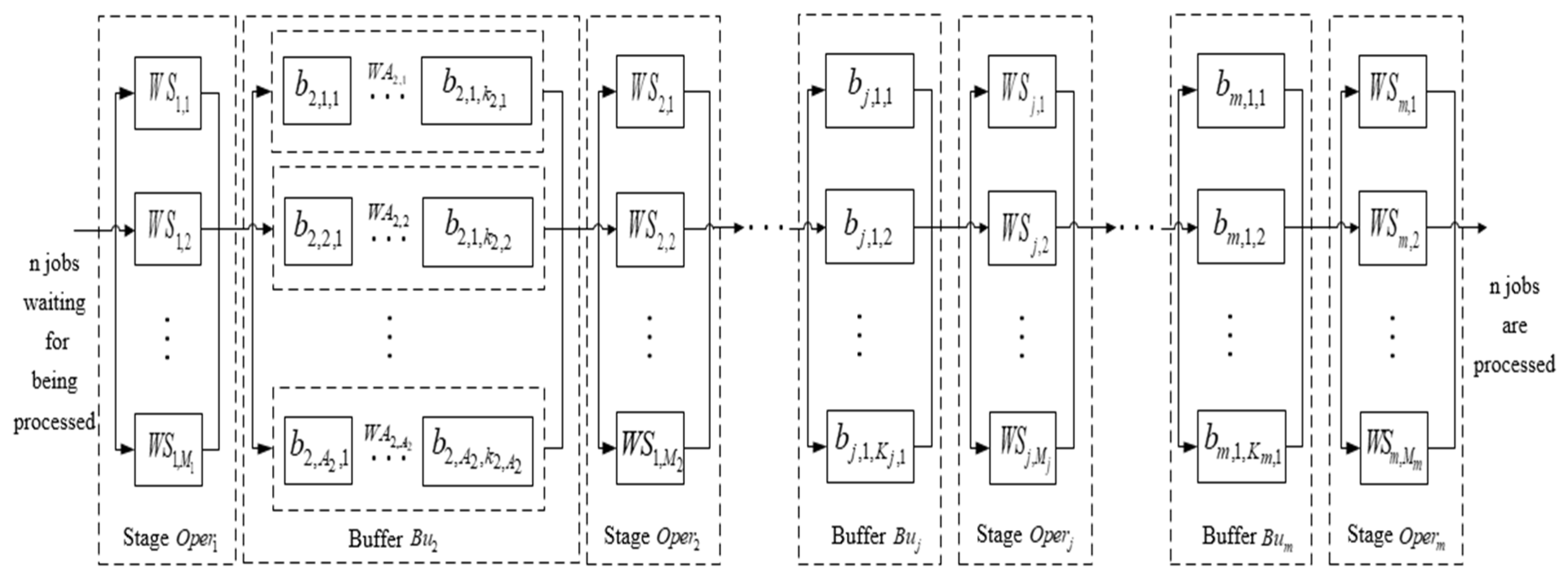
Figure 1 illustrates the scheduling problem in which n jobs are required to be processed in $m$ stages [15]. At least one stage in the $m$ stages includes multiple parallel machines. Each job is needed to be assigned one machine at each stage. Also, buffers with given capacity exist between stages. The completed job enters the buffer and waits for the availability of the next stage. If the buffer is full, the completed job of the previous stage will stay on its current machine. In this situation, the machine is unavailable and cannot process other jobs until the buffer has available spaces. The buffers contains multiple lanes, and each lane has a limited number of spaces. The job enters the lane from one side and exits the lane from the other side. The jobs that wait for processing form a waiting queue in each lane. When the job enters this buffer, it needs to select one of the lanes and enter its waiting queue. When there is an idle machine in the next stage, it is necessary to select one bus in multiple waiting queues to move out of the buffer for processing. When all the lanes of this buffer reach the upper limit of the capacity, there will also be cases where the job is blocked at the machine of the previous stage. When the job is assigned to the machine, the setup time should also be added besides the standard processing time if the property of the job did not match that of the previous job. The standard processing time of the job at each stage, the online sequence of the job in the production process and the job’s setup times, start time, and completion time at each stage can be obtained through the scheduling, so as to achieve better scheduling results.

2.2. Parameters in the Model

The parameters used in this paper are as follows:

• $n$: number of jobs to be scheduled;
• $m$: number of stages;
• $J_i$: job $i$, $i\in \{1,\dots ,n\}$;
• $Ope{r}_j$: stage $j$, $j\in \left\{1,\dots ,m\right\}$;
• $M_j$: number of machines in each stage, $j\in \left\{1,\dots ,m\right\}$;
• $W{S}_{j,l}$: machine $l$ of stage $Ope{r}_j$, $j\in \left\{1,\dots ,m\right\}$, $l\in \left\{1,\dots ,M_j\right\}$;
• $B{u}_j$: the buffer of stage $Ope{r}_j$, $j\in \left\{2,\dots ,m\right\}$;
• $A_j$: number of waiting queue in the buffer of stage $Ope{r}_j$, $j\in \left\{2,\dots ,m\right\}$;
• $B{s}_{j,a}$: the $ath$ lane of buffer $B{u}_j$ at stage $Ope{r}_j$, $j\in \left\{2,\dots ,m\right\}$, $a\in \left\{1,\dots ,A_j\right\}$;
• $K_{j,a}$: number of spaces in lane $B{s}_{j,a}$ of buffer $B{u}_j$ at stage $Ope{r}_j$, $j\in \left\{2,\dots ,m\right\}$, $a\in \left\{1,\dots ,A_j\right\}$;
• $b_{j,a,k}$: space $k$ in lane $B{s}_{j,a}$ of buffer $B{u}_j$, $j\in \left\{2,\dots ,m\right\}$, $a\in \left\{1,\dots ,A_j\right\}$, $k\in \left\{1,\dots ,K_{j,a}\right\}$;
• $W{A}_{j,a}\left(t\right)$: at time $t$, the waiting queue in the $ath$ lane $B{s}_{j,a}$ of buffer $B{u}_j$, $j\in \left\{2,\dots ,m\right\}$, $a\in \left\{1,\dots ,A_j\right\}$;
• $S_{i,j}$: the start time to process job $J_i$ at stage $Ope{r}_j$;
• $C_{i,j}$: the completion time to process job $J_i$ at stage $Ope{r}_j$;
• $T{b}_{i,j}$: the standard processing time of job $J_i$ at stage $Ope{r}_j$, $j\in \left\{1,\dots ,m\right\}$;
• $T{e}_{i,j}$: the entry time of job $J_i$ into buffer $B{u}_j$, $j\in \left\{2,\dots ,m\right\}$;
• $T{l}_{i,j}$: the departure time of job $J_i$ out of buffer $B{u}_j$, $j\in \left\{2,\dots ,m\right\}$;
• $T{o}_{i,j}$: the departure time of job $J_i$ on its machine after job $J_i$ is processed at stage $Ope{r}_j$, $j\in \left\{1,\dots ,m\right\}$;
• $T{w}_{i,j}$: the waiting time of job $J_i$ in buffer $B{u}_j$, $j\in \left\{2,\dots ,m\right\}$;
• $T{s}_{i,j,l}$: the setup time of machine $W{S}_{j,l}$ when job $J_i$ is processed on machine $W{S}_{j,l}$, $j\in \left\{2,\dots ,m\right\}$;
• $Nsr{v}_{x,i^{\prime },i^{″}}^l$: the relationship between properties of job continuously processed on machine $W{S}_{j,l}$, $i^{\prime },i^{″}\in \{1,\dots n\}$ and $i^{\prime }\ne i^{″}$.

2.3. Constraints

2.3.1. Assumptions

The variables used in this paper are as follows:

$$A{t}_{i,j,l}=\{\begin{array}{cc}1,& \begin{array}{c}\mathrm{Job} J_i \mathrm{is} \mathrm{assigned} \mathrm{to} \mathrm{be} \mathrm{processed}\\ \mathrm{on} \mathrm{machine} W{S}_{j,l} \mathrm{at} \mathrm{stage} Ope{r}_j\end{array}\\ 0,& \begin{array}{c}\mathrm{Job} J_i \mathrm{isn}’\mathrm{t} \mathrm{assigned} \mathrm{to} \mathrm{be} \mathrm{processed}\\ \mathrm{on} \mathrm{machine} W{S}_{j,l} \mathrm{at} \mathrm{stage} Ope{r}_j\end{array}\end{array}$$

(1)

$$O{A}_{i,j,a}\left(t\right)=\{\begin{array}{ll}1,& \begin{array}{l}\mathrm{At} \mathrm{time} \mathrm{t}, \mathrm{job} J_i \mathrm{is} \mathrm{in} \mathrm{waiting}\\ \mathrm{processing} \mathrm{queue} W{A}_{j,a}\left(t\right) \mathrm{at} \mathrm{stage} Ope{r}_j\end{array}\\ 0,& \begin{array}{l}\mathrm{At} \mathrm{time} t, \mathrm{job} J_i \mathrm{isn}’\mathrm{t} \mathrm{in} \mathrm{waiting}\\ \mathrm{processing} \mathrm{queue} W{A}_{j,a}\left(t\right) \mathrm{at} \mathrm{stage} Ope{r}_j\end{array}\end{array}$$

(2)

$$QB{C}_{j,a}\left(t\right)=\{\begin{array}{ll}1,& \begin{array}{l}\mathrm{At} \mathrm{time} t, \mathrm{the} \mathrm{number} \mathrm{of} \mathrm{jobs} \mathrm{in} \mathrm{lane} B{s}_{j,a} \mathrm{at} \mathrm{stage}\\ Ope{r}_j \mathrm{is} \mathrm{greater} \mathrm{than} \mathrm{zero}, \mathrm{namely}, card\left(W{A}_{j,a}\left(t\right)\right)>0\end{array}\\ 0,& \begin{array}{l}\mathrm{At} \mathrm{time} t, \mathrm{the} \mathrm{number} \mathrm{of} \mathrm{jobs} \mathrm{in} \mathrm{lane} B{s}_{j,a} \mathrm{at} \mathrm{stage}\\ Ope{r}_j \mathrm{is} \mathrm{equal} \mathrm{to} \mathrm{zero}, \mathrm{namely}, card\left(W{A}_{j,a}\left(t\right)\right)=0\end{array}\end{array}$$

(3)

2.3.2. General Constraint of Flexible Flow Shops Scheduling

The general constraint of flexible flow shops scheduling are as follows:

$${\displaystyle \sum _{l=1}^{M_j}A{t}_{i,j,l}}=1$$

(4)

$$C_{i,j}=S_{i,j}+T{b}_{i,j},i\in \left\{1,2,\cdots ,n\right\},j\in \left\{1,2,\cdots ,m\right\}$$

(5)

$$C_{i,j-1}\le S_{i,j},i\in \left\{1,2,\cdots ,n\right\},j\in \left\{1,2,\cdots ,m\right\}$$

(6)

Equation (4) indicates job $J_i$ at stage $Ope{r}_j$ can only be processed on one machine. Equation (5) constrains the relationship between the start time and completion time for job $J_i$ at stage $Ope{r}_j$. Equation (6) represents that job $J_i$ needs to complete the current stage before proceeding to the next stage. The general constraints of flexible flow shops are still valid for the multi-queue limited buffers scheduling problem in a flexible flow shop with setup times.

2.3.3. Constraints of Limited Buffers

The constraints of limited buffers are as follows:

$$T{o}_{i,j}=\{\begin{array}{cc}T{e}_{i,j+1}& j=\left\{1,\dots ,m-1\right\}\\ C_{i,j}& j=m\end{array}.$$

(7)

In Equation (7), when the job is at stage $Ope{r}_j$ ($i=\left\{1,\dots ,m-1\right\}$), the departure time of the job on the machine is equal to the entry time of the job into the buffer. When the job is at stage $Ope{r}_m$, the departure time of the job on the machine equals the completion time.

$$T{e}_{i,j}\ge C_{i,j-1},j\in \left\{2,\dots ,m\right\}.$$

(8)

Equation (8) indicates that the entry time of the job into the buffer is greater than or equal to the completion time of the job in the previous stage. If the limited buffers are blocked, the job will be retained on the machine after completing the previous stage.

$$W{A}_{j,a}\left(t\right)=\left\{J_i|O{A}_{i,j,a}\left(t\right)=1\right\}.$$

(9)

Equation (9) shows all jobs contained in the waiting queue of limited buffers at time $t$.

$$card\left(W{A}_{j,a}\left(t\right)\right)\le K_{j,a}.$$

(10)

Equation (10) denotes that at any time, the number of jobs in the waiting queue $W{A}_{j,a}$ is less than or equal to the maximum number of spaces ($K_{j,a}$) in the lane where $W{A}_{j,a}$ is located.

2.3.4. Constraints of Multi-Queue Limited Buffers

Two new constraints of Equations (11) and (12) are added based on the constraints of Equations (8) and (10).

$${\displaystyle \sum _{a=1}^{A_j}{\displaystyle \sum _{i=1}^{n}O{A}_{i,j,a}\left(t\right)}}\le n.$$

(11)

In Equation (11), when $A_j>1$, at any time, the number of jobs to be processed in the waiting queue of multi-queue limited buffers is less than or equal to the number of jobs $n$.

$${\displaystyle \sum _{a=1}^{A_j}QB{C}_{j,a}\left(t\right)}\le n.$$

(12)

In Equation (12), when $A_j>1$, at any time, the number of jobs, which can proceed to the machine of stage $Ope{r}_j$, in the waiting queue of multi-queue limited buffers is less than or equal to the number of jobs $n$.

If $\exists i^{\prime },i^{″}\in \left\{i|O{A}_{i,j,a}\left(t\right)=1\right\}$, $T{e}_{i^{\prime },j}\le T{e}_{i^{″},j}$, $T{l}_{i^{\prime },j}$ and $T{l}_{i^{″},j}$ will satisfy the following relationship

$$T{l}_{i^{\prime },j}\le T{l}_{i^{″},j}.$$

(13)

In Equation (13), when $A_j>1$, the job of the $ath$ lane must meet the requirement that the job entering the queue first should depart from the queue first.

2.3.5. Constraints of Setup Times

The constraints of setup times are as follows:

$${\displaystyle \sum _{l=1}^{M_j}\left(T{s}_{i,j,l}·A{t}_{i,j,l}\right)}+C_{i,j-1}\le S_{i,j}, i\in \left\{1,\dots ,n\right\}, l\in \left\{1,\dots ,M_j\right\}, j\in \left\{2,\dots ,m\right\}.$$

(14)

Equation (14) extends the basic constraint of Equation (6) of a flexible flow shop to obtain the relationship between setup times and start time as well as completion time. Equation (14) indicates that the start time of the current stage is greater than or equal to the completion time of the previous stage plus setup times.

$X$ denotes the number of job’s properties. $pro{p}_{x,i}$ represents the property of job $J_i$. $Pro{p}_i=\left\{pro{p}_{x,i}\right\}$ represents the collection of properties of job $J_i$, and $x\in \left\{1,\dots ,X\right\}$.

$$Nsr{v}_{x,i^{\prime },i^{″}}^l=\{\begin{array}{cc}1& pro{p}_{x,i^{\prime }}\ne pro{p}_{x,i^{″}}\\ 0& pro{p}_{x,i^{\prime }}=pro{p}_{x,i^{″}}\end{array}.$$

(15)

$J_{i^{\prime }}$ and $J_{i^{″}}$ ($i^{\prime },i^{″}\in \left\{1,\dots ,n\right\}$) are jobs continuously processed on machine $W{S}_{j,l}$. When $Nsr{v}_{x,i^{\prime },i^{″}}^l=0$, it means that when property $pro{p}_{x,i^{\prime }}$ of job $J_{i^{\prime }}$ and property $pro{p}_{x,i^{″}}$ of job $J_{i^{″}}$ are the same, no setup time is required to process the latter job on the machine. When $Nsr{v}_{x,i^{\prime },i^{″}}^l=1$, it represents that when property $pro{p}_{x,i^{\prime }}$ of job $J_{i^{\prime }}$ and property $pro{p}_{x,i^{″}}$ of job $J_{i^{″}}$ are different, the setup time is required to process the latter job on the machine.

$$T{s}_{i^{\prime },j,l}={\displaystyle \sum _{x=1}^{X}Ts{p}_{j,x}·Nsr{v}_{x,i^{\prime },i^{″}}^l}, i^{\prime },i^{″}\in \left\{1,\dots ,n\right\}, j\in \left\{2,\dots ,m\right\}, l\in \left\{1,\dots ,M_j\right\}.$$

(16)

In Equation (16), at stage $Ope{r}_j$, $Ts{p}_{j,x}$ represents the required setup times when there is a change in one property $pro{p}_{x,i}$ of two consecutively processed jobs. $TS{P}_j=\left\{Ts{p}_{j,x}\right\}$ denotes the collection of setup times when there is a change in the property of two consecutively processed jobs at stage $Ope{r}_j$, and $x\in \left\{1,\dots ,X\right\}$. $T{s}_{i^{\prime },j,l}$ is the required setup time when several properties of job $J_{i^{\prime }}$ processed on machine $W{S}_{j,l}$ at stage $Ope{r}_j$ are different from those of the previous job processed on the same machine.

Other constraints are as follows. Uninterruptible constraint: if the job has been started on the machine, it cannot be interrupted until the production process on the machine is completed. Machine availability constraint: all machines in the scheduling are available at production time. Time simplification constraint: not to consider the time of jobs transferred among spaces in the multi-queue limited buffers, and the time of jobs transferred between machines in front and back stages, that is to say, only consider the processing time of the job processed in each stage and setup times when the property of jobs processed successively on the machine is changed.

2.4. Evaluation Index of the Scheduling Result

• Makespan

$$C_{max}=\max \left\{C_{i,m}\right\}, i\in \left\{1,2,\dots ,n\right\}.$$

(17)

In Equation (17), $C_{max}$ indicates the maximum completion time of all jobs processed at the last stage, which is also the time for all jobs to complete the process.

• Waiting processing time for total job

$$TWIP={\displaystyle \sum _{j=2}^m{\displaystyle \sum _{i=1}^n\left(S_{ij}-C_{i,j-1}\right)}}.$$

(18)

In Equation (18), the waiting time of the job is from the completion moment $C_{i,j-1}$ of job $J_i$ at stage $Ope{r}_{j-1}$ to the start moment $S_{ij}$ at the next stage $Ope{r}_j$. $TWIP$ represents the sum of the waiting times of all jobs processed in the entire production. In the production shop of limited buffers, the waiting time of each job between stages is equal to the sum of time for the job staying on the buffer ($T{l}_{i,j}-T{e}_{i,j}$), blocking time of the job on the machine ($T{e}_{i,j}-C_{i,j-1}$), and setup times (${\displaystyle \sum _{l=1}^{M_j}\left(T{s}_{i,j,l}·A{t}_{i,j,l}\right)}$).

• Idle time for total machine

$$TWT={\displaystyle \sum _{j=1}^m{\displaystyle \sum _{l=1}^{M_j}\left(\left(\max \left\{T{o}_{i,j}\cdot A{t}_{i,j,l}\right\}-\min \left\{S_{i,j}\cdot A{t}_{i,j,l}\right\}\right)-{\displaystyle \sum _{i=1}^n\left(T{b}_{i,j}\cdot A{t}_{i,j,l}\right)}\right)}}.$$

(19)

The idle time for the machine in Equation (19) represents the time between the start time of the first job and completion time of the last job on each machine. $TWT$ is the sum of idle time for all machines.

• Total device availability

$$FUR=\frac{{\displaystyle \sum _{j=1}^m{\displaystyle \sum _{i=1}^n\left(T{b}_{i,j}\right)}}}{{\displaystyle \sum _{j=1}^m{\displaystyle \sum _{l=1}^{M_j}\left(\max \left\{T{o}_{i,j}\cdot A{t}_{i,j,l}\right\}-\min \left\{S_{i,j}\cdot A{t}_{i,j,l}\right\}\right)}}}.$$

(20)

In Equation (20), $FUR$ represents the total device availability of all machines in a flexible flow shop, which is the ratio of the effective processing time of all machines to the occupied time span of the machine. This time span starts from the first job processed on the machine to the last job that is finished and has left the machine.

• Total machine setup times

$$TS={\displaystyle \sum _{i=1}^n{\displaystyle \sum _{j=1}^m{\displaystyle \sum _{l=1}^{M_j}\left(T{s}_{i,j,l}·A{t}_{i,j,l}\right)}}}.$$

(21)

In Equation (21), $TS$ is the sum of all stages’ setup times in a flexible flow shop.

• Total job blocking time

$$TPB={\displaystyle \sum _{i=1}^n{\displaystyle \sum _{j=2}^m\left(T{e}_{i,j}-C_{i,j-1}\right)}}.$$

(22)

In Equation (22), $TPB$ is the sum of blocking time of all jobs stuck on the machine due to the buffers being full after all jobs finish the processing in a flexible flow shop.

3. Improved Compact Genetic Algorithm

In the evolution of standard CGA, new individuals are generated based on probability distribution of the probabilistic model, and individuals conforming to the evolutionary trend are selected to update the distribution probability. The elements in the model, namely the probability values, represent the distribution of feasible solutions. The continuously accumulated optimization information in the evolution is reflected in the probability values of the probabilistic model. The CGA adopts the single individual to update the probabilistic model in each generation, and the new individual of each generation is also generated in the model. After several generations, if one of the probability values on the model’s column (or row), which controlled the generation of individual gene fragments, is extremely large, it leads to similar genes appearing in the same position of new individuals generated in later evolutions, decreasing the diversity of new individuals. As the individuals generated from the probabilistic model will update the model conversely, the probability values will further increase. When elements (probability values) in the probabilistic model all become 0 or 1, the CGA will terminate the evolution process. Therefore, it is difficult for the CGA to jump out of the local extremum once it falls into this situation. Afterward, the overall trend for evolution is irreversible, leading to a premature convergence of the algorithm. As such, if only an expanding the number of new individuals generated by the model is considered, the optimization effect of the algorithm cannot be significantly improved, and the advantage of the CGA in the fast search will be lost. The probabilistic model and the process of generating new individuals from the model were explored to prevent the prematurity of the CGA and improve the quality and diversity of new individuals. First, the distribution of probability values in a column (or a row) that were related to gene fragments of new individuals in the probabilistic model were determined, and then the probability density function of the Gaussian distribution was introduced to map the probabilistic model from the original one to the new one. Under the premise of keeping the probability values’ distribution of the original probabilistic model unchanged, the search ability of feasible solutions could be expanded, thereby developing the diversity of new individuals.

3.1. Establishing and Initializing the Probabilistic Model

The probabilistic model was responsible for counting and recording the distribution of genes in the individual after the evolution of the algorithm. According to the individual coding information, namely online sequence and machine assignment, the n × n matrix $P^L$ was established as the online-sequence probabilistic model of the CGA to optimize the scheduling online sequence. In the probabilistic model, the 1st to nth rows corresponded to jobs $J_1$ to $J_i$, and the 1st to nth columns corresponded to individuals 1 to n. $P_{i,s}^1$ indicated the probability of job $J_i$ appearing at position $s$ of the online processing queue.

The probabilistic model was initialized by a uniform assignment. This method directly set the equal probability of each job appearing at each position, providing a more balanced optimization starting point for the algorithm. It used the uniform assignment to initialize the probabilistic model $P$, namely $\forall (i,s), P_{i,s}^1=1/n$, which could expand the search range of the algorithm’s feasible solution. In addition, it was restricted by the constraint that $\forall (s), {\displaystyle \sum _{i=1}^n{P}_{i,s}^1}=1$.

3.2. Mapping the Original Probabilistic Model to the New Probabilistic Model

Some scholars used information entropy to evaluate the distribution of probability values in the probabilistic model [16]. This approach is not quite sensitive to the distribution of probability values. This study adopted the method of calculating the standard deviation of probability values in the probabilistic model to assess the probability distribution in the original probabilistic model so as to judge and evaluate the ability of the current model to search for feasible solutions.

The ICGA consisted of two models: the original probabilistic model $P^L$ and the new probabilistic model $F^L$. The element $P_{i,s}^L$ in the probabilistic model referred to the probability of job $J_i$ appearing at position $s$ in online processing queue.

The probability value distribution in $P^L$ was judged by calculating each column of standard deviation ${\sigma }_s{}^L$ in the original probability model $P^L$. Meanwhile, the standard deviation-based threshold value ${\sigma }^T$ which started the mapping operation was set to judge whether the probability density function of the Gaussian distribution can be started to map $P^L$ to the new probability model $F^L$. When ${\sigma }_s{}^L>{\sigma }^T$, mapping the $P^L$ to the $F^L$ using the probability density function of the Gaussian distribution shown in Equation (23). Then, a new feasible solution $I^L$ (new individual) of the problem was generated in accordance with the $F^L$. The original probability model $P^L$ was updated through this new feasible solution. After that, this new feasible solution was applied to update the $P^L$. The scope of searching a feasible solution was magnified through expanding the ability of the $P^L$ to select new feasible solutions.

$$f(x|{\mu }_s^L,{\sigma }_s^L)=\frac{1}{{\sigma }_s^L\cdot \sqrt{2\pi }}{e}^{-\frac{{\left(x-{\mu }_s^L\right)}^2}{2{\sigma }_s^L{}^2}}.$$

(23)

Equation (23) is the probability density function of the Gaussian distribution, where ${\mu }_s^L$ is the expectation value of the $sth$ column in the probabilistic model $P^L$, and the calculation formula is shown in Equation (24). ${\sigma }_s{}^L$ is the standard deviation of the $sth$ column in the probabilistic model $P^L$, and the calculation formula is shown in Equation (25). The size of the standard deviation determines the degree of steepness or flatness of the Gaussian distribution curve. The smaller the $\sigma$, the steeper the curve; and the larger the $\sigma$, the flatter the curve. With the evolution of the CGA, the distribution of probability values in the probabilistic model decreases, and the value of $\sigma$ becomes larger (a probability value is dominant, while others are small and far from the average value). Further, the selection range after the mapping will become larger.

$${\mu }_s^L={\displaystyle \sum _{i=1}^n{P}_{i,s}^L}·i$$

(24)

$${\sigma }_s{}^L=\sqrt{\frac{1}{n}·{{\displaystyle \sum _{s=1}^n\left(P_{i,s}^L-\frac{1}{n}\right)}}^2}.$$

(25)

At the beginning of evolution $P_{i,s}^L=1/n$, and the initial value of ${\sigma }_s{}^L$ is 0. If the value of ${\sigma }_s{}^L$ is too small, the Gaussian distribution curve is too steep, the probability value after mapping is smaller. As such, the standard deviation adjustment parameter $\xi$ is added to Equation (25) to obtain the standard deviation ${\sigma }_s{}^{\xi L}$ after adjustment in Equation (26).

$${\sigma }_s{}^{\xi L}=\xi ·\sqrt{\frac{1}{n}·{{\displaystyle \sum _{s=1}^n\left(P_{i,s}^L-\frac{1}{n}\right)}}^2}$$

(26)

$$\xi =\frac{n·max\left\{P_{i,s}^L\right\}}{{\displaystyle \sum _{i=1}^n{P}_{i,s}^L}-max\left\{P_{i,s}^L\right\}}.$$

(27)

In Equation (27), the standard deviation adjustment parameter $\xi$ satisfies the constraints: when $max\left\{P_{i,s}^L\right\}=1$ or ${\displaystyle \sum _{i=1}^n{P}_{i,s}^L}-max\left\{P_{i,s}^L\right\}=0$, $\xi =\sqrt{n}$.

After determining the probability density function of the Gaussian distribution corresponding to each column element in the $P^L$, this function was used to obtain the corresponding probability value $G{P}_{i,s}^L$ of each probability value $P_{i,s}^L$ in this column in the new probabilistic model $F^L$. The specific operations were: first, determine the range $\left[X_1,X_2\right]$ for each probability value $P_{i,s}^L$ on the X axis, where $X_1={\displaystyle \sum _{h=1}^{i-1}{P}_{h,s}^L}$, $X_2={\displaystyle \sum _{h=1}^i{P}_{h,s}^L}$. Then, determine the position of expectation value ${\mu }_s^L$ on the X axis. Finally, the corresponding probability value $G{P}_{i,s}^L$ of probability value $P_{i,s}^L$ in the $F^L$ is obtained by using Equation (28)

$$G{P}_{i,s}^L=\{\begin{array}{cc}\left|f(X_1)-f(X_2)\right|& {\mu }_s^L\notin \left[X_1,X_2\right]\\ 2·f({\mu }_s^L)-f(X_1)-f(X_2)& {\mu }_s^L\in \left[X_1,X_2\right]\end{array}.$$

(28)

After all the columns in the $P^L$ have been mapped, the probability values in each column of the new probabilistic model $F^L$ were normalized to ensure that the sum of the probability values in each column was 1. Then, the roulette was used to choose the positions of jobs which were arranged in the processing queue based on the $F^L$, so as to generate new individuals in more diversities. The superior individual among new individuals was chosen to update the original probabilistic model $P^L$ through Equation (29).

$$P_{i,s}^{L+1}=\left(1-\frac{\beta }{n}\right)·P_{i,s}^L+\frac{\beta }{n}·St, St=\{\begin{array}{cc}1& Gen{e}_s=i\\ 0& Gen{e}_s\ne i\end{array}$$

(29)

where $St$ is the learning coefficient; $n$ is the number of jobs to be processed; and $\beta$ is the adjustment override of the learning rate. In each generation, the superior individual is selected to update the probabilistic model. The genetic value $Gen{e}_s$ in the individual represents the sequential position of job $J_i$ in online processing queue. Equation (29) shows that when the value of $Gen{e}_s$ is i, the probability value $P_{i,s}^1$ in the $sth$ column of the model which combines with learning coefficient $St$ further increases the probability of job $J_i$ being chosen on the position $s$ in the online processing queue. In addition, other probability values of this column subtract $\frac{\beta }{n}·P_{i,s}^L$.

3.3. Encoding and Decoding of New Individuals

Based on the probabilistic model, $NP$ new individuals were generated. The process of generating each new individual was: in the probabilistic model $P^L$, based on the probability $P_{i,s}$, the genetic value of individual from the 1st to nth referred to the probability $P_{i,s}$ of the job $J_i$ which appeared on the $sth$ position. The job numbers were chosen on the basis of roulette in turn, that is, the job online order. In the process of individual decoding, the individual genetic value was decoded into the online processing sequence of $n$ jobs in the first stage.

3.4. Procedure of the ICGA

Step 1: Initialize probabilistic model $P^L$. According to the principle of the maximum entropy, the probabilistic model $P^L$ is initialized, where $\forall (i,s)P_{i,s}^L=1/n$. Meanwhile, the evolutionary generation is set as $L=0$.

Step 2: Map the probability value $P_{i,s}^L$ in the original probabilistic model $P^L$ to the new probabilistic model $F^L$. Calculate the standard deviation ${\sigma }_s{}^L$ of the probability value of the $sth$ column in the original probabilistic model $P^L$, and judge whether ${\sigma }_s{}^L$ is larger than the threshold value ${\sigma }^T$ for initiating the mapping operation. If ${\sigma }_s{}^L\le {\sigma }^T$, the probability value of the $sth$ column in the $P^L$ is taken as the $sth$ column probability value in the new probabilistic model $F^L$. If ${\sigma }_s{}^L>{\sigma }^T$, execute Step 3.

Step 3: Calculate the expectation value ${\mu }_s^L$ of the probability value of the $sth$ column in the original probabilistic model $P^L$. Determine its corresponding probability density function of the Gaussian distribution, and calculate the probability value $G{P}_{i,s}^L$ in the new probabilistic model $F^L$ corresponding to each probability value $P_{i,s}^L$ in the $sth$ column.

Step 4: Repeat Step 2 until all the columns in the original probabilistic model $P^L$ are all mapped into the new probabilistic model $F^L$.

Step 5: Generate new individuals based on the new probabilistic model $F^L$. Through the roulette, the individual genetic sampling values are selected in turn according to the probability values of each column in the $F^L$, and these genetic values represent the positions of the jobs to be machined in the online queue. Once a job is selected, it no longer participates in the subsequent selection, while the unselected jobs go on to take part in the selection process until all jobs are arranged so as to generate a new individual. After that, $NP$ new individuals $I_1,I_2,\dots ,I_{NP}$ are generated.

Step 6: $NP$ new individuals are decoded and the fitness function value for each new individual can be calculated.

Step 7: Compare the fitness function values of $NP$ new individuals, and select the optimal individual $I_{better}$ among them, and its fitness function value is $f_{better}$.

Step 8: Judge whether $f_{better}$ is better than the fitness function value $f_{best}$ of the historically optimal individual $I_{best}$. If $f_{better}$ is better than $f_{best}$, replace $I_{best}$ with $I_{better}$ and replace $f_{best}$ with $f_{better}$.

Step 9: The historically optimal individual $I_{best}$ is used to update the probabilistic model $P^L$, and the update operation is performed according to Equation (29). At the same time, evolutionary generation L is processed as $L=L+1$.

Step 10: Judge whether the updated original probabilistic model $P^L$ converges, that is, whether all probability values of model $P^L$ are 1 or 0. If the convergence is met, the historically optimal individual $I_{best}$ is output and the evolution process ends. Otherwise, execute Step 11.

Step 11: Judge whether the evolutionary generation L reaches the set maximum evolutionary generation $L_{\max }$. If $L=L_{\max }$, the historically optimal individual $I_{best}$ is output and the evolution process ends. Otherwise, Step 2 is performed again.

The flowchart of the ICGA is shown in Figure 2.

4. Local Scheduling Rules for Multi-Queue Limited Buffers

In order to reduce the setup times and reduce the impact of setup times on the scheduling process, this paper has developed a variety of local scheduling rules to guide the distribution of jobs for the process of entering and exiting multi-queue limited buffers. When the job enters the multi-queue limited buffer, the local scheduling rules employ the remaining capacity of max queue buffer (RCMQB) rule. When the job leaves the multi-queue limited buffer, the local scheduling rules use the shortest setup time (SST) rule, the first available machine (FAM) rule, and the first-come first-served (FCFS) rule, of which the SST rule is a priority [17].

4.1. Rules for Jobs Entering Multi-Queue Limited Buffers

• Max queue buffer capacity remaining rule

When $\exists C_{i,j-1}$ and $t=C_{i,j-1}$,

$$\begin{array}{c}Mc{a}_{i,j}\left(t\right)=\left\{B{s}_{j,a}|max\left\{K_{j,a}-card\left(W{A}_{j,a}\left(t\right)\right)|\left(K_{j,a}-card\left(W{A}_{j,a}\left(t\right)\right)>0\right)\right\}\right\}\\ j\in \left\{2,\dots ,m\right\}\end{array}$$

(30)

where $Mc{a}_{i,j}\left(t\right)$ is the set of lane $B{s}_{j,a}$ that the job in the previous stage $Ope{r}_{j-1}$ can access. The difference between the maximum number of spaces ($K_{j,a}$) of each lane $B{s}_{j,a}$ and the number of jobs in the waiting queue $W{A}_{j,a}$ in this lane is the remaining capacity (available space) of lane $B{s}_{j,a}$ at the current stage. When the job finishes the previous stage, namely when $t=C_{i,j-1}$, the job enters the lane with the largest remaining capacity. When $card\left(Mc{a}_j\left(t\right)\right)=0$, it indicates there is no remaining space in the current lane. When $card\left(Mc{a}_j\left(t\right)\right)>1$, it illustrates that multiple lanes can be entered.

4.2. Rules for Jobs Leaving Multi-Queue Limited Buffers

When the job exits the buffer and is assigned to the machine, in the case of an available machine $W{S}_{j,l}$ and several jobs are waiting in the buffer, that is, the number of the selectable jobs to be processed in the multi-queue limited buffers is greater than 1 (${\displaystyle \sum _{a=1}^{A_j}QB{C}_{j,a}\left(t\right)}>1$). In the course of assigning jobs, the job with the minimum setup time ($\left\{J_i|min\left(T{s}_{i^{\prime },j,l}\right)\right\}$) is processed according to the SST rule. If the number of jobs with the minimum setup time is greater than 2, the job with the longest waiting time in the buffer ($\left\{J_i|max\left\{\left(t-T{e}_{i,j}\right)|\left\{i|O{A}_{i,j,a}\left(t\right)=1\right\}\right\}\right\}$) is selected for processing in accordance with the first in first out (FIFO) rule. In the case of available machines and only one job waiting to be processed, that is, the number of selectable jobs to be processed in the multi-queue limited buffers is equal to 1 (${\displaystyle \sum _{a=1}^{A_j}QB{C}_{j,a}\left(t\right)}=1$), the SST rule is used to select the machine with the minimum setup time in the course of assigning machines. If the number of selectable machines is greater than 2, the job is machined on the basis of the FAM rule. The multimachine-and-multi-job case is a combination of the aforementioned conditions.

5. Simulation Experiment

The ICGA was implemented using MATLAB 2016a simulation software, running on the PC with Windows 10 operating system, Core i5 processor, 2.30 GHz Central Processing Unit (CPU), and 6 GB memory. The multi-queue limited buffers scheduling problems in a flexible flow shop with setup times originate from the production practice of bus manufacturers. It is a complex scheduling problem. As standard examples are not available at present, the standard data of a flexible flow shop scheduling problem (FFSP) was employed to discuss and analyze the parameters in the improved compact genetic algorithm, so as to determine the optimal parameter [18]. In addition, multiple groups of large-scale and small-scale data were used to test the effect of the improved method on the optimization ability of the standard CGA. Furthermore, the instance data of multi-queue limited buffers scheduling in a flexible flow shop with setup times were used to verify the optimal performance of the ICGA for solving such problems.

5.1. Analysis of Algorithm Parameters

The parameter values of the algorithm had a significant effect on the algorithm’s optimization performance. The ICGA has three key parameters: threshold value ${\sigma }^T$ that started the mapping operation, adjustment override of the learning rate $\beta$, and thr number of new individuals generated in each generation $NP$. The FFSP standard examples of a d-class problem with five stages and 15 jobs in the 98 standard examples proposed by Carlier and Neron were applied to test each parameter. The example j15c5d3 was used to illustrate the orthogonal experiment. Three parameters, each with four levels (see

Table 1. Level of each parameter.

Parameter	Level
	1	2	3	4
${\sigma }^T$	5	10	15	20
$\beta$	1.0	1.5	2.0	2.5
$NP$	2	3	4	5

), were taken for orthogonal experiments with the scale of L₁₆ (4³) [19]. The algorithm ran 20 times in each group of experiments. The average time of makespan ($\overline{C_{max}}$) was used as an evaluation index.

Through experiments, we can see that the influence of the change of each parameter on the performance of the algorithm is shown in Figure 3. From the figure we can see that $\beta$ and $NP$ had a greater impact on the performance of the algorithm, and ${\sigma }^T$ had the least impact on the performance of the algorithm. The best combination of parameters was: ${\sigma }^T$ = 10, $\beta$ = 1.5, $NP$ = 4.

5.2. Optimization Performance Testing on the ICGA

In order to study the impact of the improved method (which is based on the probability density function of the Gaussian distribution mapping) on the optimization performance of the CGA, the ICGA was compared with CGA, bat algorithm (BA) [20] and whale optimization algorithm (WOA) [21]. These algorithms are the currently emerging intelligent optimization algorithms and are widely used in the field of optimization and scheduling [22,23,24]. In the BA, the number of individuals in the population $NP$ = 30, pulse rate γ = 0.9, search pulse frequency range [F_min, F_max] = [0, 2]. In the WOA, the number of individuals in the population $NP$ = 30. Each algorithm ran 30 times on each group of data. The maximum evolutionary generation of four algorithms was set to 500 generations. The average makespan $\overline{C_{max}}$ and the average running time $\overline{T_{cpu}}$ were used as the evaluation metrics.

5.2.1. Small-Scale Data Testing

The test data are from the 98 standard examples proposed by Carlier and Neron based on the standard FFSP. The set of examples was divided into five classes. According to the difficulty of solving the examples, the set of examples was divided into two categories by Neron et al. [25]: easy to solve and difficult to solve. Four groups of easy examples (j15c5a1, j15c5a2, j15c5b1, and j15c5b2) and four groups of difficult examples (j15c10c3, j15c10c4, j15c5d4, and j15c5d5) were chosen to test the ICGA so as to better evaluate the optimization performance of the ICGA for small-scale data. The test results are shown in

Table 2. Small-scale data test results.

Standard Example	LB	BA		WOA		CGA		ICGA
		$\overline{{\mathit{C}}_{\mathit{m}\mathit{a}\mathit{x}}}$	$\overline{{\mathit{T}}_{\mathit{c}\mathit{p}\mathit{u}}}(\mathbf{s})$	$\overline{{\mathit{C}}_{\mathit{m}\mathit{a}\mathit{x}}}$	$\overline{{\mathit{T}}_{\mathit{c}\mathit{p}\mathit{u}}}(\mathbf{s})$	$\overline{{\mathit{C}}_{\mathit{m}\mathit{a}\mathit{x}}}$	$\overline{{\mathit{T}}_{\mathit{c}\mathit{p}\mathit{u}}}(\mathbf{s})$	$\overline{{\mathit{C}}_{\mathit{m}\mathit{a}\mathit{x}}}$	$\overline{{\mathit{T}}_{\mathit{c}\mathit{p}\mathit{u}}}(\mathbf{s})$
j15c5a1	178	178	16.324	178	4.018	178	0.652	178	0.671
j15c5a2	165	165	16.474	165	4.029	165	0.738	165	0.754
j15c5b1	170	170	15.585	170	3.887	170	0.669	170	0.682
j15c5b2	152	152	15.767	152	3.863	152	0.636	152	0.710
j15c10c3	141	148.14	31.722	148.77	8.008	150.30	0.768	147.56	1.007
j15c10c4	124	132.86	48.289	133.28	8.056	135.65	0.764	132.26	1.121
j15c5d4	61	87.16	17.679	87.02	4.267	89.57	0.471	86.13	0.758
j15c5d5	67	82.03	17.368	82.28	4.296	84.65	0.435	81.72	0.756

.

In the table, LB represents the lower bound of makespan for the examples, whose optimal value was given by Santos and Neron [25,26]. It can be seen from Table 2 that even if the data size was small, the average running time of the CGA and ICGA under each group of data was significantly shorter than that of the BA and WOA. This indicates that CGA and ICGA have the advantages of the convergence speed of optimization. In terms of the optimization performance of small-scale data, the four algorithms did not have significant differences. But overall, the optimization effect of the ICGA on small-scale data was still the best among the four algorithms. The ICGA has achieved better solutions than the other three algorithms when solving all four groups of difficult examples (the four algorithms all reached the lower bound of makespan when solving the easy examples). Especially, compared with the CGA, when solving two groups of examples of the j15c5d class, the average relative error obtained by the ICGA was reduced by 5.64% and 4.37%, respectively. This shows that the optimization effect of the ICGA is greatly improved from the CGA when solving small-scale data.

5.2.2. Large-Scale Data Testing

Six groups of data, including 80 jobs with four stages, 80 jobs with eight stages, and 120 jobs with four stages, were used to test the optimization performance of the ICGA in solving large-scale complex problems. The test results are shown in

Table 3. Large-scale data test results.

Instance Number	BA		WOA		CGA		ICGA
	$\overline{{\mathit{C}}_{\mathit{m}\mathit{a}\mathit{x}}}$	$\overline{{\mathit{T}}_{\mathit{c}\mathit{p}\mathit{u}}}(\mathbf{s})$	$\overline{{\mathit{C}}_{\mathit{m}\mathit{a}\mathit{x}}}$	$\overline{{\mathit{T}}_{\mathit{c}\mathit{p}\mathit{u}}}(\mathbf{s})$	$\overline{{\mathit{C}}_{\mathit{m}\mathit{a}\mathit{x}}}$	$\overline{{\mathit{T}}_{\mathit{c}\mathit{p}\mathit{u}}}(\mathbf{s})$	$\overline{{\mathit{C}}_{\mathit{m}\mathit{a}\mathit{x}}}$	$\overline{{\mathit{T}}_{\mathit{c}\mathit{p}\mathit{u}}}(\mathbf{s})$
j80c4d1	1459.84	49.351	1465.12	17.485	1477.56	11.722	1455.44	13.731
j80c4d2	1367.44	49.735	1372.40	18.549	1385.16	12.595	1364.48	14.717
j80c8d1	1811.68	106.187	1813.88	51.967	1842.56	16.174	1814.28	19.078
j80c8d2	1822.56	104.954	1830.48	51.485	1851.92	16.079	1828.96	19.767
j120c4d1	2132.08	78.779	2138.04	38.171	2196.92	23.859	2139.88	28.942
j120c4d2	2243.52	79.821	2250.41	39.275	2306.52	24.221	2246.04	29.642

.

As can be seen from the table, when solving the problem of large-scale data, the advantages of the CGA and ICGA in the speed of optimization were more obvious. Especially when solving two groups of examples of j80c8d class, the average running time of CGA and ICGA was significantly smaller than the BA and WOA. It can be seen from the test results of the first four groups of examples that when the number of processes was increased from four to eight, the average running time of the BA and the WOA was greatly increased. On the other hand, although the average running time of the CGA and the ICGA was also increased, the rate of increase was small. This indicates that CGA and ICGA are suitable for solving the problem of scheduling optimization with large data scale with many processes. In general, when solving the problem of large-scale data, the optimization performance of the BA and ICGA was better than that of the WOA and CGA. As for the aspect of optimization speed, the average running time of the BA was much larger than the other three algorithms under every group of data.

It can also be seen from the table that although the CGA had the fastest optimization speed under each group of large-scale data, its optimization performance was also the worst among the four algorithms. And as the size of the data increased, the gap between the CGA and the other three algorithms was getting larger. This is mainly because the CGA uses roulette to select gene fragments in the probabilistic model when generating new individuals. In the initial stage of the probabilistic model, the probability of each gene fragment being selected is $1/n$. When the size of the data is large (n = 80 and n = 120), the initial probability value of each gene fragment in the probability matrix becomes small (1/8 and 1/120). Further, in the process of evolution, the probability value of the unselected gene fragment will be reduced again, and the probability value of the selected gene fragment will be increased. This will lead to the probability values of certain gene fragments that are much larger than the probability values at other locations after several generations of evolution. Although this will make the evolution speed of the algorithm faster, it will also lead to a decline in the diversity of new individuals generated by the probabilistic model, which means the premature convergence of the algorithm. Compared with the CGA, when solving the problems of each group of large-scale data, the optimization effect of the ICGA was greatly improved. This indicates that the ICGA, to some extent, overcame the problem that the CGA was easy to prematurely converge.

By testing the four algorithms using large-scale and small-scale data, we can conclude that compared with the CGA, the ICGA has stronger capability to continuously evolve and jump out of the local extremum while maintaining the characteristic of fast convergence of the CGA. The ICGA, to some extent, overcomes the problem that the CGA is easy to prematurely converge. At the same time, compared with the BA and the WOA, for either small-scale data or large-scale data, the ICGA has an obvious advantage in optimization speed. Thus, the ICGA is suitable for solving the complicated problem of scheduling optimization with many processes.

5.3. Instance Test on Multi-Queue Limited Buffers in Flexible Flow Shops with Setup Times

5.3.1. Establishing Simulation Data

The simulation data of the production operations in the body shop and paint shop of the bus manufacturer were established as follows.

1. Parameters in the shop model

The body shop of the bus manufacturer is a rigid flow shop with multiple production lines, which can be simplified into one production stage. The production of the paint shop is simplified to three stages [27]. The simulation data for scheduling include four stages, namely $\left\{Ope{r}_1,Ope{r}_2,Ope{r}_3,Ope{r}_4\right\}$, whose parallel machine $\left\{M_j\right\}$ is $\left\{3,2,3,2\right\}$. The buffer between the body shop and the paint shop is a multi-queue limited buffer. As such, the buffer of stage $Ope{r}_2$ in the scheduling simulation data is set to the multi-queue limited buffer. The number of lanes in buffer $B{u}_2$ of stage $Ope{r}_2$ is equal to 2, namely $A_2$ = 2. The number of spaces in lane $B{s}_{2,1}$ is 2, namely $K_{2,1}$ = 2, and that of buffer $B{s}_{2,2}$ is 2, namely $K_{2,2}$ = 2. That is to say, the multi-queue limited buffers have two lanes and each lane has two spaces.

In the production of the paint shop, it is necessary to clean the machine and adjust production equipment if the model and color of the buses that are successively processed on the machine are different. Therefore, the simulation process uses the changes in the model and color as the basis for calculating setup times.

Table 4. Model parameters.

	Parameter	Description	Value
Parameters of limited buffers	$A_2$	Number of lanes in buffer $B{u}_2$ of stage $Ope{r}_2$	2
	$K_{2,1}$	Capacity of lane $B{s}_{2,1}$	2
	$K_{2,2}$	Capacity of lane $B{s}_{2,2}$	2
	$K_{3,1}$	Capacity of limited buffer $B{u}_3$ of stage $Ope{r}_3$	1
	$K_{4,1}$	Capacity of limited buffer $B{u}_4$ of stage $Ope{r}_4$	1
Parameters of setups times	$Ts{p}_{2,1}$	Setup times when the model of buses processed successively on a parallel machine of stage $Ope{r}_2$ changes	4
	$Ts{p}_{2,2}$	Setup times when the color of buses processed successively on a parallel machine of stage $Ope{r}_2$ changes	4
	$Ts{p}_{3,1}$	Setup times when the model of buses processed successively on a parallel machine of stage $Ope{r}_3$ changes	5
	$Ts{p}_{3,2}$	Setup times when the color of buses processed successively on a parallel machine of stage $Ope{r}_3$ changes	5
	$Ts{p}_{4,1}$	Setup times when the model of buses processed successively on a parallel machine of stage $Ope{r}_4$ changes	3
	$Ts{p}_{4,2}$	Setup times when the color of buses processed successively on a parallel machine of stage $Ope{r}_4$ changes	3

shows that the setup times parameters are set when the model and color of the buses that are processed successively on the machine changed. When the bus is assigned to the machine of the next stage from the buffer, the setup times of the machine is calculated using Equation (16).

2. Parameters of processing the object

The information of the bus model and color properties is shown in

Table 5. Information of bus model and color properties.

Bus Property	${\mathit{J}}_1$	${\mathit{J}}_2$	${\mathit{J}}_3$	${\mathit{J}}_4$	${\mathit{J}}_5$	${\mathit{J}}_6$	${\mathit{J}}_7$	${\mathit{J}}_8$	${\mathit{J}}_9$	${\mathit{J}}_{10}$	${\mathit{J}}_{11}$	${\mathit{J}}_{12}$
Model $Pro{p}_1$	$Typ{e}_1$	$Typ{e}_2$	$Typ{e}_3$	$Typ{e}_2$	$Typ{e}_1$	$Typ{e}_3$	$Typ{e}_1$	$Typ{e}_2$	$Typ{e}_3$	$Typ{e}_1$	$Typ{e}_2$	$Typ{e}_3$
Color $Pro{p}_2$	$Colo{r}_1$	$Colo{r}_1$	$Colo{r}_2$	$Colo{r}_2$	$Colo{r}_3$	$Colo{r}_3$	$Colo{r}_1$	$Colo{r}_1$	$Colo{r}_2$	$Colo{r}_3$	$Colo{r}_2$	$Colo{r}_3$

. The sum of bus properties is 2, namely $X=2$. $Pro{p}_1$ represented the model property of the bus, while $Pro{p}_2$ denoted the color property of the bus. The value of model property ($PropValu{e}_1$) is $\left\{BusTyp{e}_1,BusTyp{e}_2,BusTyp{e}_3\right\}$, and the value of color property ($PropValu{e}_2$) is $\left\{BusColo{r}_1,BusColo{r}_2,BusColo{r}_3\right\}$. It is assumed that two successively processed buses on machine of stage $W{S}_{2,1}$ are buses $J_1$ and $J_5$. If model properties were as follows: $pro{p}_{1,1}$ = $BusTyp{e}_1$ and $pro{p}_{1,5}$ = $BusTyp{e}_1$, and color properties are as follows: $pro{p}_{2,1}$ = $BusColo{r}_1$ and $pro{p}_{2,5}$ = $BusColo{r}_3$, then $pro{p}_{1,1}$ = $pro{p}_{1,5}$, $pro{p}_{2,1}$ $\ne$ $pro{p}_{2,5}$. Hence, $Nsr{v}_{2,1,5}^2=1$. Using Equation (16), the setup time can be obtained as follows: $T{s}_{5,2,2}$ = $Ts{p}_{2,2}$ = 4. And the

Table 6. Standard processing time for bus production.

	${\mathit{J}}_1$	${\mathit{J}}_2$	${\mathit{J}}_3$	${\mathit{J}}_4$	${\mathit{J}}_5$	${\mathit{J}}_6$	${\mathit{J}}_7$	${\mathit{J}}_8$	${\mathit{J}}_9$	${\mathit{J}}_{10}$	${\mathit{J}}_{11}$	${\mathit{J}}_{12}$
$Ope{r}_1$	8	11	15	19	10	16	12	21	22	13	20	14
$Ope{r}_2$	30	38	28	25	26	36	20	24	22	32	35	34
$Ope{r}_3$	34	38	44	42	52	40	46	48	35	36	45	50
$Ope{r}_4$	42	36	26	24	34	30	28	32	38	40	44	22

shows the standard processing time for bus production.

5.3.2. Simulation Scheme

The scheduling problem of the bus manufacturer was investigated by using the ICGA, BA, WOA, and standard CGA as the global optimization algorithm, combined with local dispatching rules in the multi-queue limited buffers. This study further analyzed the optimization performance of the ICGA combined with local dispatching rules in solving the multi-queue limited buffers scheduling problems in a flexible flow shop with setup times. A total of eight groups of simulation schemes were designed, in which schemes 1–4 employed the FIFO rule as their local dispatching rules, and schemes 5–8 adopted the RCMQB rule when entering the buffer and used the SST rule, FAM rule, and FCFS rule as local dispatching rules when leaving the buffer. Among them, the SST rule was the priority. The information of the eight sets of simulation schemes is shown in

Table 7. The eight groups of the simulation program.

Simulation Scheme	Global Optimization Algorithm	Local Dispatching Rules
Scheme 1	BA	FIFO
Scheme 2	WOA	FIFO
Scheme 3	CGA	FIFO
Scheme 4	ICGA	FIFO
Scheme 5	BA	RCMQB; SST, FAM, FCFS
Scheme 6	WOA	RCMQB; SST, FAM, FCFS
Scheme 7	CGA	RCMQB; SST, FAM, FCFS
Scheme 8	ICGA	RCMQB; SST, FAM, FCFS

.

5.3.3. Simulation Results and Analysis

1. Evaluation index of scheduling results

In the optimization process, makespan $C_{max}$ was used as the fitness function value of the global optimization algorithm. Meanwhile, a number of evaluation indexes related to the actual production line were established, including $T_{cpu}$, $TWIP$, $TWT$, $FUR$, $TS$ and $TPB$. Except $FUR$, the smaller the values, the better the remaining evaluation indexes.

Eight sets of simulation schemes were run 30 times. The average of 30 simulation results is presented in

Table 8. Evaluation index comparison of scheduling results of eight schemes.

Evaluation Index		Scheme 1	Scheme 2	Scheme 3	Scheme 4	Scheme 5	Scheme 6	Scheme 7	Scheme 8
$C_{max}$	Optimum	296	295	297	295	288	288	290	286
	Worst	307	305	309	304	303	300	302	300
	Average	301.12	303.16	305.76	300.56	293.56	295.60	299.84	292.32
	variance	18.56	8.96	11.74	9.06	12.48	5.07	8.69	6.86
$T_{cpu}$	Optimum	529.15	103.35	14.30	15.29	503.83	113.27	14.264	15.64
	Worst	587.99	144.61	15.23	16.24	600.83	149.73	15.39	16.77
	Average	551.61	122.57	14.32	15.08	559.48	134.35	14.62	15.32
	variance	325.24	339.50	0.041	0.06	425.57	81.53	0.05	0.18
$TWIP$	Optimum	630	642	623	623	625	605	613	611
	Worst	768	730	745	750	734	707	718	713
	Average	691.52	689.72	698.32	681.96	660.88	656.48	672.64	647.44
	variance	824.88	550.12	958.45	764.27	781.56	421.86	795.19	635.52
$TWT$	Optimum	229	253	250	251	202	202	204	203
	Worst	358	321	347	343	282	278	309	302
	Average	282.81	282.96	287.56	285.60	240.36	235.48	255.40	248.04
	variance	673.44	428.41	514.16	564	543.59	276.83	493.68	517.95
$FUR$	Optimum	86.26%	85.03%	85.18%	85.43%	87.67%	87.62%	87.56%	87.59%
	Worst	80.36%	80.17%	80.54%	80.25%	83.59%	83.79%	82.91%	83.16%
	Average	83.58%	83.41%	83.14%	83.34%	85.68%	85.93%	84.94%	85.88%
	variance	0.05%	0.01%	0.02%	0.02%	0.02%	0.00%	0.01%	0.01%
$TS$	Optimum	110	121	126	115	105	108	108	98
	Worst	153	164	167	160	141	137	151	144
	Average	137.64	139.12	148.52	138.43	121.36	119.76	125.60	120.76
	variance	123.31	103.59	130.24	114.40	66.15	45.86	91.08	73.62
$TPB$	Optimum	73	73	77	74	70	72	75	72
	Worst	122	109	118	113	118	99	110	104
	Average	94.42	93.04	94.88	93.28	87.8	85.16	87.64	95.21
	variance	165.12	71.55	97.82	99.16	129.44	48.21	69.59	74.36

. As shown in the table, under the principle of adopting the same global optimization algorithm, compared with schemes 1–4, each metric of schemes 5–8 has been improved to some extent, except the $T_{cpu}$. Among the metrics, the optimization improvement of $TWIP$, $TS$ and $TPB$ is obvious. This is mainly because schemes 5–8 adopted RCMQB rules when entering multi-queue limited buffers, which can allocate resources of multi-queue limited buffers more reasonably and reduce the occurrence of blocking. The SST rule, the FAM rule and the FCFS rule were adopted when leaving the buffer, which can more effectively control the jobs to select the machine with the least change of properties among multiple machines for processing. This was beneficial to reduce the setup times. Further, $TWIP$ is equal to the sum of the time for the job staying on the buffer, the blocking time of the job and setup times, so these three evaluation indexes were significantly improved. The reduction in blocking time and setup times will lead to the reduction in the makespan of the whole process and the reduction of the idle time for machines. Therefore, $C_{max}$, $TWT$ and $FUR$ of schemes 5–8 were also optimized to some extent. From the table we can also see that compared with the schemes 1–4, although the $T_{cpu}$ of the schemes 5–8 had all increased, the rate of increase was small. This indicates that the complicated local rules adopted in schemes 5–8 can made full use of the capacity of the multi-queue limited buffers and effectively reduced the blocking time and setup times. At the same time, the running time costs were small and did not have much impact on the speed of the algorithm.

The comparison among schemes 1–4 or schemes 5–8 show that the running speed of the CGA and ICGA was significantly faster than that of the BA and WOA. The average running time of the BA reached 555.56 s, which is obviously not suitable for solving practical problems. In terms of optimization performance, under two different local dispatching rules, the optimization effect of ICGA for $C_{max}$ was the best among the four algorithms. Specially, compared with the CGA, the optimization effect of the ICGA was significantly improved. The above results show that the ICGA, to some extent, overcame the problem that the CGA was easy to prematurely converge while maintaining the fast running speed of the CGA. This is mainly because in the early stage of evolution, there is no large probability value in the probabilistic model. Thus, the ICGA was still evolving as the procedure of the CGA. In this way, the ICGA maintained the advantage that the CGA can converge quickly in the early stage of evolution. In the later stage of evolution, when falling into the local extremum, the ICGA mapped the original probabilistic model to the new probabilistic model through the probability density function of the Gaussian distribution. In this way, while keeping probability values’ distribution of the original probabilistic model unchanged, ICGA’s searching ability of feasible solutions was expanded, and the diversity of population individuals was improved. Therefore, the algorithm could jump out of the local extremum and continued to evolve.

Through the above analysis, it can be concluded that compared with the other seven schemes, the combination of the ICGA and local dispatching rules adopted in scheme 8 was the best for reducing setup times of the machine, and it effectively decreased the blocking effect of the limited buffers, more reasonably arranged the jobs in and out of the multi-queue limited buffer, and orderly assigned the processing tasks. Various evaluation metrics were improved, and the problem of multi-queue limited buffers scheduling problems in a flexible flow shop with setup times was more effectively solved.

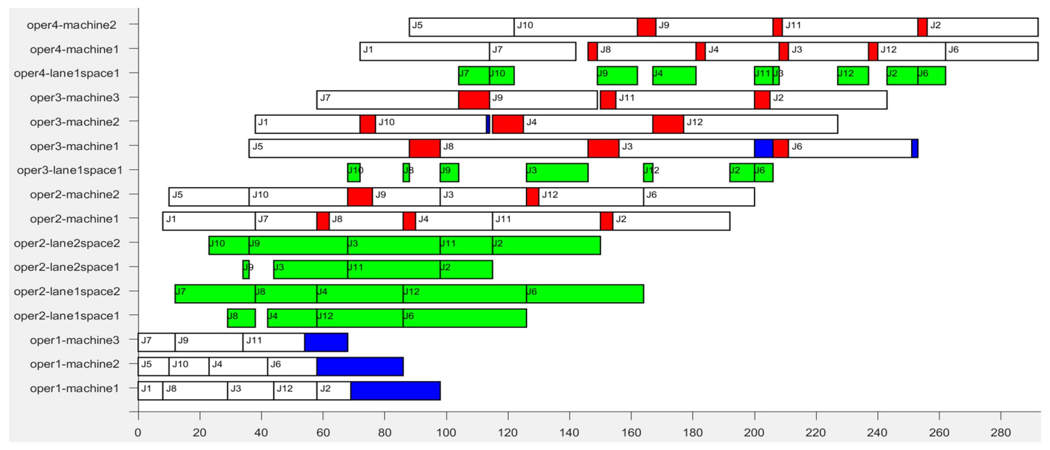
2. Gantt chart analysis of scheduling result

Figure 4 is the Gantt chart of the scheduling result of scheme 8, with time axis as the abscissa and machine of each stage as the ordinate. The green part indicates the residence time of the bus in the buffer. The red part indicates the setup times when the successively-processed buses are with different properties. The blue part denotes the blocking time of the bus on the machine after the completion of the process. The processing route of $J_3$ was $\left\{W{S}_{1,1},b_{2,2,1},b_{2,2,2},W{S}_{2,2},b_{3,1,1},W{S}_{3,1},b_{4,1,1},W{S}_{4,1}\right\}$. In Figure 4, we can see that at time $t$ = 44, $J_3$ completed the processing on machine $W{S}_{1,1}$ of stage $Ope{r}_1$ (the competition time of $J_3$ was 44, namely $C3,1$ = 44). At this time, the first lane $B{s}_{2,1}$ of buffer $B{u}_2$ had two jobs waiting to be processed ($J_8$ and $J_4$), that is to say, $W{A}_{2,1}\left(t\right)=\left\{J_8,J_4\right\}$, $card\left(W{A}_{2,1}\left(t\right)\right)$ = 2. The second lane $B{s}_{2,2}$ of buffer $B{u}_2$ had one job waiting to be processed ($J_9$), that is to say, $W{A}_{2,2}\left(t\right)=\left\{J_9\right\}$, $card\left(W{A}_{2,2}\left(t\right)\right)$ = 1. The capacity of lane $B{s}_{2,1}$ was 2 ($K_{2,1}$ = 2), $card\left(W{A}_{2,1}\left(t\right)\right)\le K_{2,1}$. And the capacity of lane $B{s}_{2,2}$ was 2 ($K_{2,2}$ = 2), $card\left(W{A}_{2,2}\left(t\right)\right)\le K_{2,2}$. Both of them satisfy the constraint of Equation (10) of the limited buffers. At this time, based on the RCMQB rule which regulates the job’s access to the buffer, we can obtain $Mc{a}_{3,2}\left(t\right)=\left\{B{s}_{2,2}\right\}$ from Equation (26). The $J_3$ was assigned to space $b_{2,2,1}$ in lane $B{s}_{2,2}$ of stage $Ope{r}_2$, waiting to be processed at stage $Ope{r}_2$. The entry time of the bus into the buffer ($T{e}_{3,2}$) was equal to $C3,1$, which satisfied the constraint of Equation (8) of limited buffers.

At time $t$ = 68, $J_9$ left the space $b_{2,2,2}$ in lane $B{s}_{2,2}$, and the departure time out of the buffer ($T{l}_{9,2}$) was 68. At the same time, $J_3$ was assigned to the space $b_{2,2,2}$, waiting to be processed on the machine of stage $Ope{r}_2$. At time $t$ = 98, $T{l}_{3,2}$ = 98, $J_3$ also departed from the buffer, and $T{l}_{9,2}<T{l}_{3,2}$, satisfying the constraint of Equation (13). From the Gantt chart drawn from scheduling results, it can be seen that the constraint of Equation (12) was always met during the use of multi-queue limited buffers.

Further analysis of the process that $J_3$ left the buffer is as follows. When $t$ = 98, machine $W{S}_{2,2}$ completed the processing of $J_9$, so that machine $W{S}_{2,2}$ was available. At this time, $J_{12}$ on space $b_{2,1,2}$ in lane $B{s}_{2,2}$ was waiting for processing, and $J_3$ on space $b_{2,2,2}$ was also waiting for processing. According to the bus’s property information in Table 3, in regard to machine $W{S}_{2,2}$, if we choose to process $J_{12}$, the setup time ($T{s}_{12,2,2}$) will be equal to $Ts{p}_{2,2}$, namely $T{s}_{12,2,2}$ = $Ts{p}_{2,2}$ = 4; if we choose to process $J_3$, the setup time ($T{s}_{3,2,2}$) will be 0, namely $T{s}_{3,2,2}$ = 0. In accordance with the SST rule that controls the job leaving the buffer, $J_3$ was chosen to process.

3. Analysis of scheduling evolution

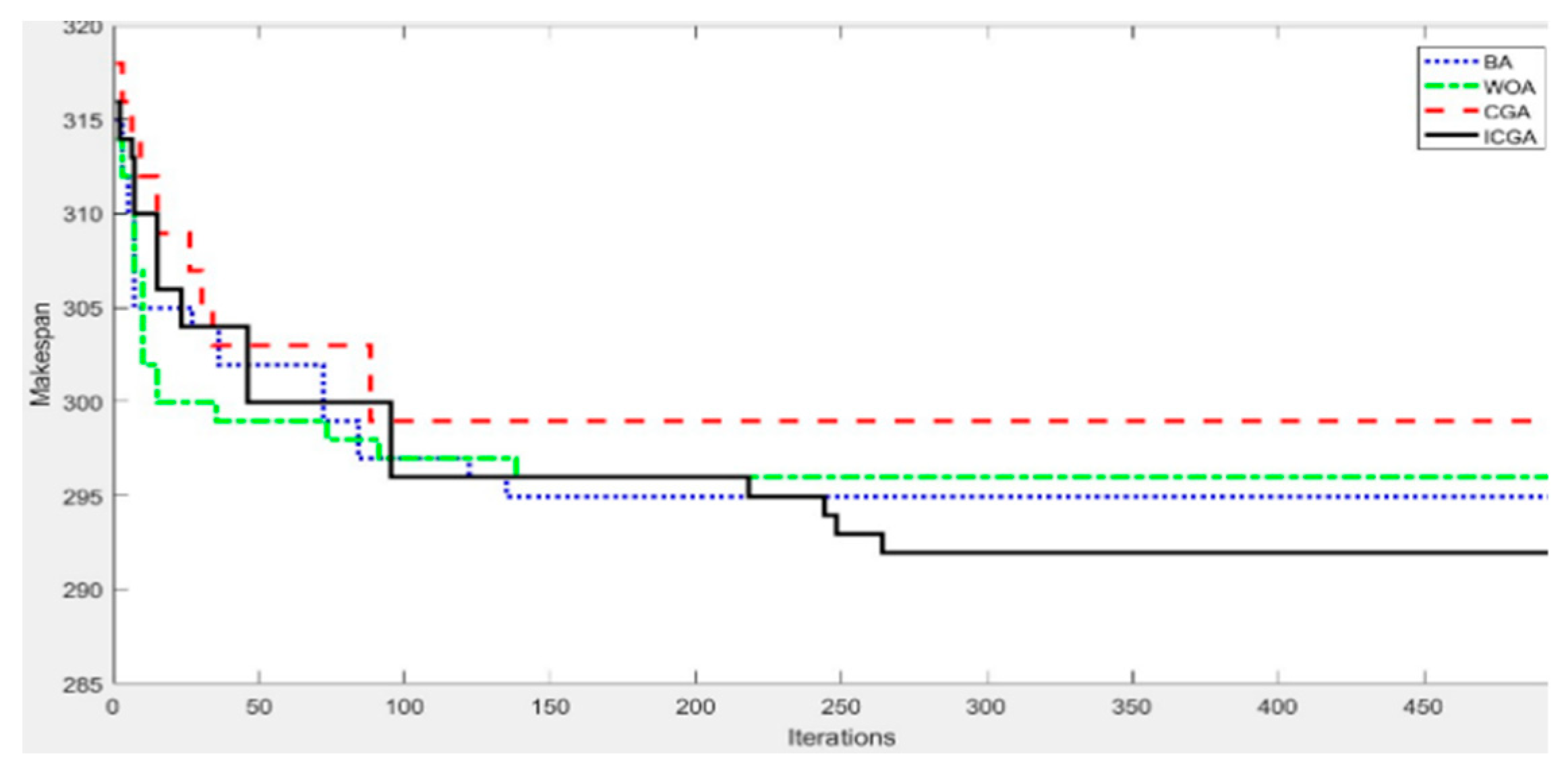
Figure 5 shows the relationship between fitness value and training iterations of schemes 5–8. As can be seen, the BA and WOA converged quickly at the initial stage of the evolution. This is mainly due to the fact that the initial numbers of population of the BA and WOAs ($NP$ = 30) were much larger than that of the CGA and ICGAs ($NP$ = 4). This means a relatively strong ability for searching the solution space. However, with the increase in evolutional iterations, the search ability of the BA and the WOA gradually deterioratesdand they fell into the local extremum in the 135th and 139th generations, respectively. Although the CGA should be good at fast search, the distribution of probability values in the probabilistic model all decreased with evolution, and thus and the search performance on the solution space decreased. The algorithm stopped evolving at the 87th generation, falling into the local extremum. On the other hand, the ICGA had the similar fast search performance as the CGA during the initial stage and encountered evolutionary stagnation at the 94th generation. But as evolution continues, the ICGA started the mapping operation to reactivate the algorithm’s evolutionary ability and found for the optimal solution in the 263th generation.

Figure 6 shows the relationship between fitness value and running time of schemes 5–8. As can be seen from the figure, the running speed of CGA and ICGA was very fast, but the CGA fell into the local extremum at 4 s. The optimization speed of the BA was the slowest among the four algorithms, and its optimal solution was 299 during the 35 s running time. From the figure, we can also see that the fitness value of the ICGA was the best among the four algorithms at the same CPU time. And the time used by the ICGA to get the same fitness value was the least among the four algorithms. The ICGA maintained the advantage that the CGA can converge quickly in the early stage of evolution. In the later stage of evolution, when falling into the local extremum, the ICGA improved the diversity of individuals in the population by mapping the original probabilistic model to a new probabilistic model, so that the algorithm could jump out of the local extremum and continue to evolve.

4. Statistical analysis of scheduling results

Figure 7 shows the makespan $C_{max}$ of schemes 5–8 running 10 times separately. For scheme 7, the average value of makespan $C_{max}$ in 10 tests was 298.1, which was the worst among the four schemes. Although scheme 5 could sometimes obtain better results, the results obtained in 10 tests were not stable enough and were with large fluctuations, easily falling into the local extremum sometimes. Its average value of 10 tests was 295.2. Compared with the other three schemes, the results obtained by the scheme 6 were relatively stable. However, its average result was poor, at 296.3. The average value of the test results of scheme 8 was 292.3, which was the best of all the schemes. The fluctuations of the curve indicate that the magnitude of the change in the results of scheme 8 in 10 tests is small. This shows that when solving multi-queue limited buffers scheduling problems in a flexible flow shop with setup times, compared with the CGA, the ICGA has not only greatly improved the optimization performance, but also improved the stability of the optimization results.

6. Conclusions

This study explored the multi-queue limited buffers scheduling problems in a flexible flow shop with setup times in a bus manufacturer. The study proposed an ICGA for global optimization to better improve the global optimization results, aiming at the shortcomings of the CGA that it is easy to fall into the local extremum and rapidly stops evolving. This algorithm employed the probability density function of the Gaussian distribution to map the original probabilistic model to a new probabilistic model so as to enhance the evolutionary vigor of the CGA. The job was processed on the specified online sequence in accordance with the individual decoding. Considering the impact of multi-queue limited buffers, the problems of the job into and out of the buffer during the subsequent scheduling were emphasized. When the job enters the buffer, the remaining capacity of buffers should be taken into account to reduce machining blocking and stagnation. When the job leaves the buffer and is assigned to the machine at the next stage, it is influenced by the setup times. In this study, the setup time of the machine was calculated based on the change in the properties of successively processed jobs. The SST rule was used to reduce the setup times. Finally, the findings of simulation experiments proved that combining the ICGA with local dispatching rules could better solve the multi-queue limited buffers scheduling problems in a flexible flow shop with setup times.

References

- Zhao, F.Q.; Tang, J.X.; Wang, J.B.; Jonrinaldi, J. An improved particle swarm optimization with a linearly decreasing disturbance term for flow shop scheduling with limited buffers. Int. J. Comput. Integr. Manuf. 2014, 27, 488–499. [Google Scholar] [CrossRef]
- Ventura, J.A.; Yoon, S.H. A new genetic algorithm for lot-streaming flow shop scheduling with limited capacity buffers. J. Intell. Manuf. 2013, 24, 1185–1196. [Google Scholar]
- Han, Z.H.; Sun, Y.; Ma, X.F.; Lv, Z. Hybrid flow shop scheduling with finite buffers. Int. J. Simul. Process Model. 2018, 13, 156–166. [Google Scholar]
- Zeng, M.; Long, Q.Y.; Liu, Q.M. Cellular automata variation particles warm optimization algorithm for batch scheduling. In Proceedings of the 2012 Second International Conference on Intelligent System Design and Engineering Application, Sanya, Hainan, China, 6–7 January 2012; IEEE: New York, NY, USA, 2012. [Google Scholar]
- Zhang, P.W.; Pan, Q.K.; Liu, J.Q.; Duan, J.H. Hybrid artificial bee colony algorithms for flowshop scheduling problem with limited buffers. Comput. Integr. Manuf. Syst. 2013, 19, 2510–2511. [Google Scholar]
- Zhang, S.C.; Wong, T.N. Studying the impact of sequence-dependent set-up times in integrated process planning and scheduling with E-ACO heuristic. Int. J. Prod. Res. 2016, 54, 4815–4838. [Google Scholar] [CrossRef]
- Shen, L.; Dsuzere, P.; Neufeld, J.S. Solving the flexible job shop scheduling problem with sequence-dependent setup times. Eur. J. Oper. Res. 2018, 265, 503–516. [Google Scholar] [CrossRef]
- Tran, T.T.; Araujo, A.; Bech, J.C. Decomposition methods for the parallel machine scheduling problem with setups. INFORMS J. Comput. 2016, 28, 83–95. [Google Scholar] [CrossRef]
- Vallada, E.; Ruiz, R. A genetic algorithm for the unrelated parallel machine scheduling problem with sequence dependent setup times. Eur. J. Oper. Res. 2011, 211, 612–622. [Google Scholar] [CrossRef] [Green Version]
- Benkalai, I.; Rebaine, D.; Gagné, C.; Baptiste, P. Improving the migrating birds optimization metaheuristic for the permutation flow shop with sequence-dependent set-up times. Int. J. Prod. Res. 2017, 55, 6145–6157. [Google Scholar] [CrossRef]
- An, Y.J.; Kim, Y.D.; Choi, S.W. Minimizing makespan in a two-machine flowshop with a limited waiting time constraint and sequence-dependent setup times. Comput. Oper. Res. 2016, 71, 127–136. [Google Scholar]
- Lenstra, J.K.; Kan, A.; Brucker, P. Complexity of machine scheduling problems. Stud. Integer Program. 1977, 1, 343–362. [Google Scholar]
- Harik, G.R.; Lobo, F.G.; Goldberg, D.E. The compact genetic algorithm. IEEE Trans. Evol. Comput. 1999, 3, 287–297. [Google Scholar] [CrossRef] [Green Version]
- Rafael, D.S.; Carlos, E.L.; Heitor, L. Template matching in digital images using a compact genetic algorithm with elitism and mutation. J. Circuits Syst. Comput. 2010, 19, 91–106. [Google Scholar]
- Sharifi, R.; Anvari-Moghaddam, A. A Flexible Responsive Load Economic Model for Industrial Demands. Processes 2019, 7, 147. [Google Scholar] [CrossRef]
- Tran, V.; Ramkrishna, D. Simulating Stochastic Populations. Direct Averaging Methods. Processes 2019, 7, 132. [Google Scholar] [CrossRef]
- Gao, Z.W.; Saxen, H.; Gao, C.H. Data-Driven Approaches for Complex Industrial Systems. IEEE Trans. Ind. Inform. 2013, 9, 2210–2212. [Google Scholar] [CrossRef]
- Gao, Z.W.; Ding, S.X.; Cecati, C. Real-time Fault Diagnosis and Fault Tolerant. IEEE Trans. Ind. Electron. 2015, 62, 3752–3756. [Google Scholar] [CrossRef]
- Han, Z.H.; Zhu, Y.H.; Ma, X.F.; Chen, Z.L. Multiple rules with game theoretic analysis for flexible flow shop scheduling problem with component altering times. Int. J. Model. Identif. Control 2016, 26, 1–18. [Google Scholar] [CrossRef]
- Yang, X.S. A new metaheuristic bat-inspired algorithm. In Nature Inspired Cooperative Strategies for Optimization; Springer: Berlin, Germany, 2010; pp. 65–74. [Google Scholar]
- Mirjalili, S.; Lewis, A. The whale optimization algorithm. Adv. Eng. Softw. 2016, 95, 51–67. [Google Scholar] [CrossRef]
- Luo, Q.F.; Zhou, Y.Q.; Xie, J.; Ma, M.; Li, L.L. Discrete bat algorithm for optimal problem of permutation flow shop scheduling. Sci. World J. 2014, 2014. [Google Scholar] [CrossRef]
- Zhang, J.J.; Li, Y.G. An improved bat algorithm and its application in permutation flow shop scheduling problem. Adv. Mater. Res. 2014, 1049, 1359–1362. [Google Scholar] [CrossRef]
- Jiang, T.H.; Zhang, C.; Zhu, H.Q.; Gu, J.C.; Deng, G.L. Energy-efficient scheduling for a job shop using an improved whale optimization algorithm. Mathematics 2018, 6, 220. [Google Scholar] [CrossRef]
- Neron, E.; Baptiste, P.; Gupta, J. Solving hybrid flow shop problem using energetic reasoning and global operations. Omega 2001, 29, 501–511. [Google Scholar] [CrossRef]
- Santos, D.L.; Hunsucker, J.L.; Deal, D.E. Global lower bounds for flow shop with multiple processors. Eur. J. Oper. Res. 1995, 80, 112–120. [Google Scholar] [CrossRef]
- Kim, M.K.; Narasimhan, R. Designing Supply Networks in Automobile and Electronics Manufacturing Industries: A Multiplex Analysis. Processes 2019, 7, 176. [Google Scholar] [CrossRef]
Figure 1.
Model for the multi-queue limited buffers scheduling problems in a flexible flow shop.
Figure 2.
The flowchart of ICGA.
Figure 3.
Trend chart of the algorithm’s performance impacted by each parameter.
Figure 4.
Gantt chart of the scheduling result of the ICGA.
Figure 5.
Relationship between fitness value and training iterations of schemes 5–8.
Figure 6.
Relationship between fitness value and Running time of schemes 5–8.
Figure 7.
Results of 10 instance tests.