Distinct and Quantitative Validation Method for Predictive Process Modelling in Preparative Chromatography of Synthetic and Bio-Based Feed Mixtures Following a Quality-by-Design (QbD) Approach


Abstract
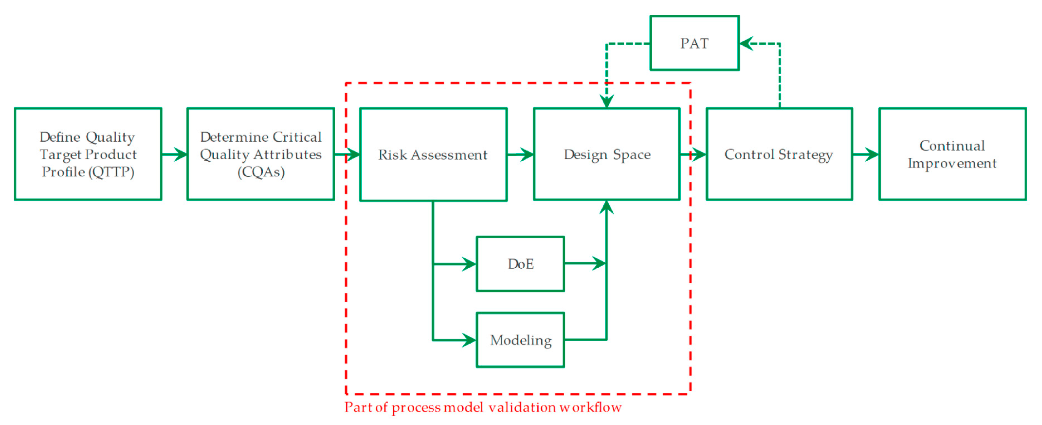
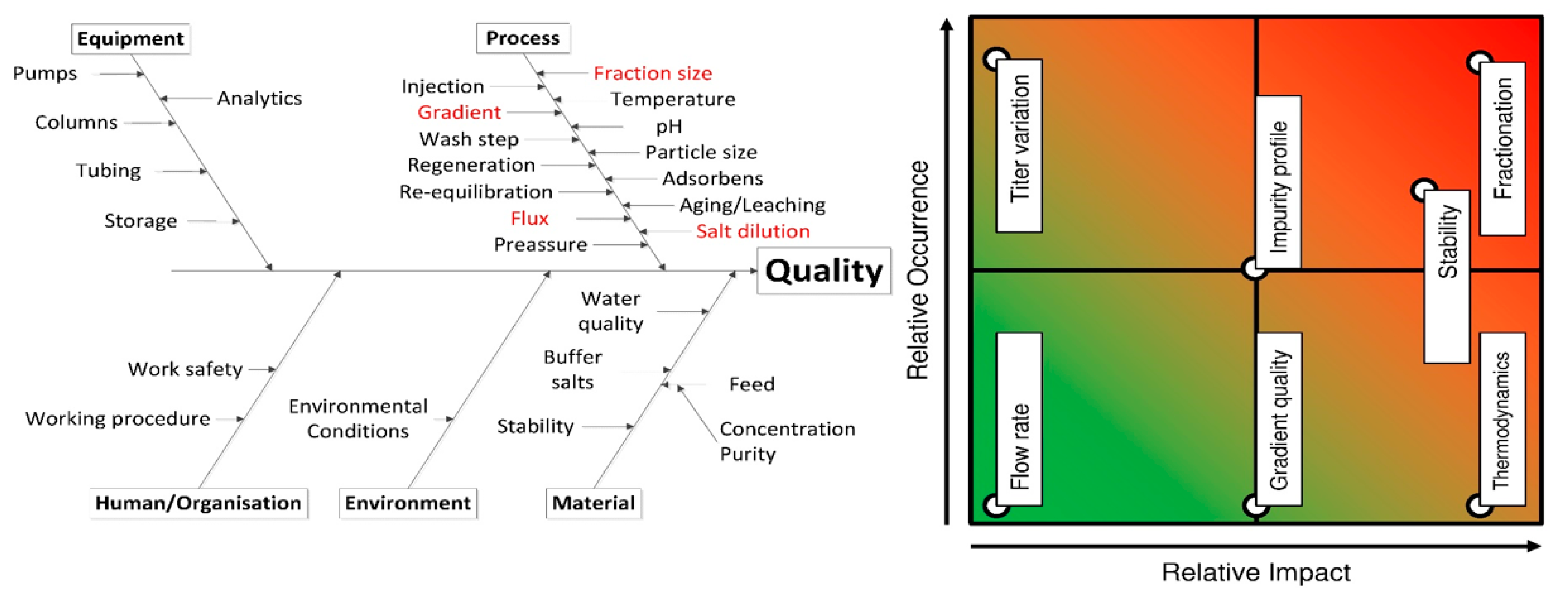
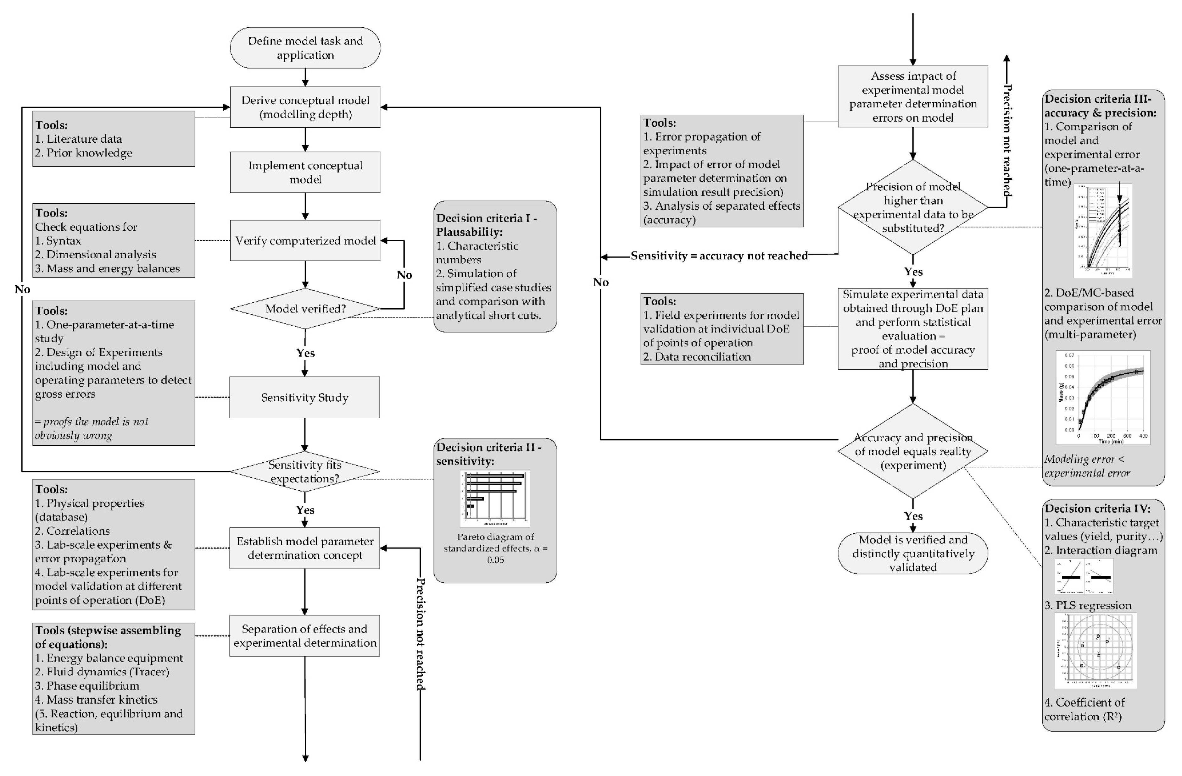
:1. Introduction
2. Modeling Chromatography: General Rate Model
3. Materials and Methods
3.1. Feed Mixtures, Buffers, and Stationary Phases
3.2. Instruments and Devices
3.3. Analytics
3.4. Experimental Validation Runs
3.5. Software Tools
4. Model Parameter Determination
4.1. Voidage, Porosity, and Axial Dispersion Coefficient
4.2. Mass Transfer Coefficient
4.3. Pore Diffusion Coefficient
4.4. Adsorption Isotherm
5. Process Model Development and Validation: Case Studies
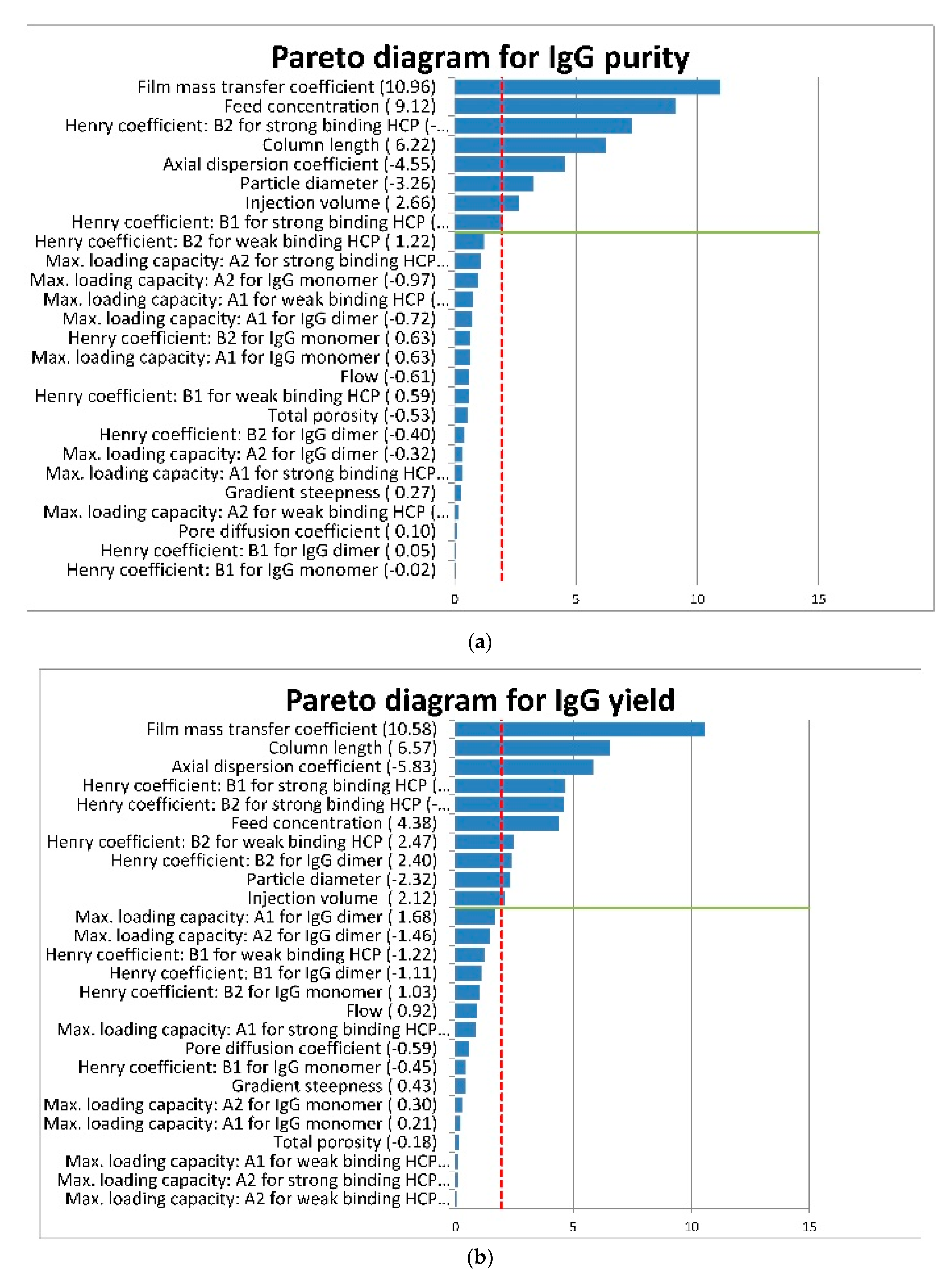
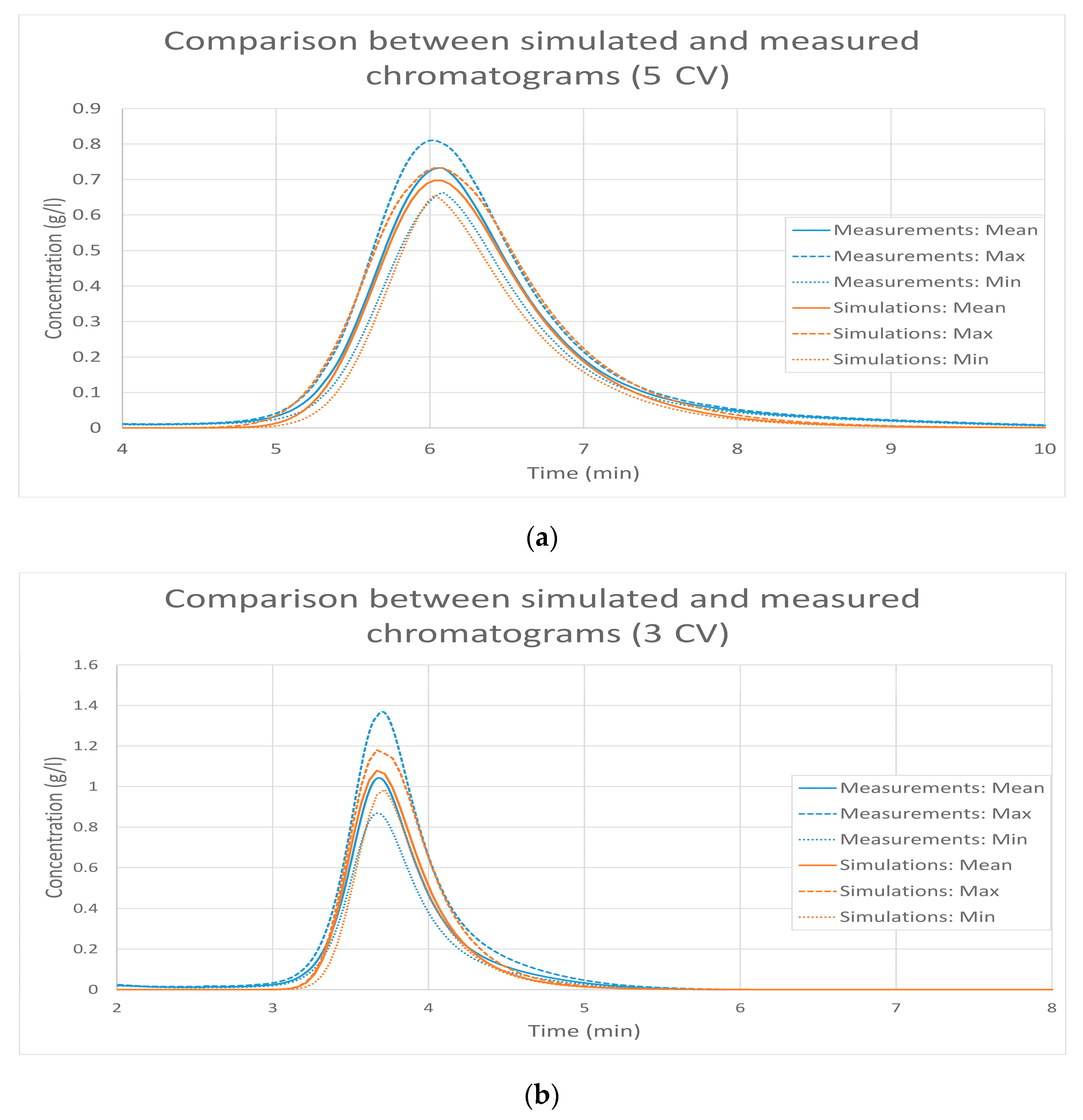
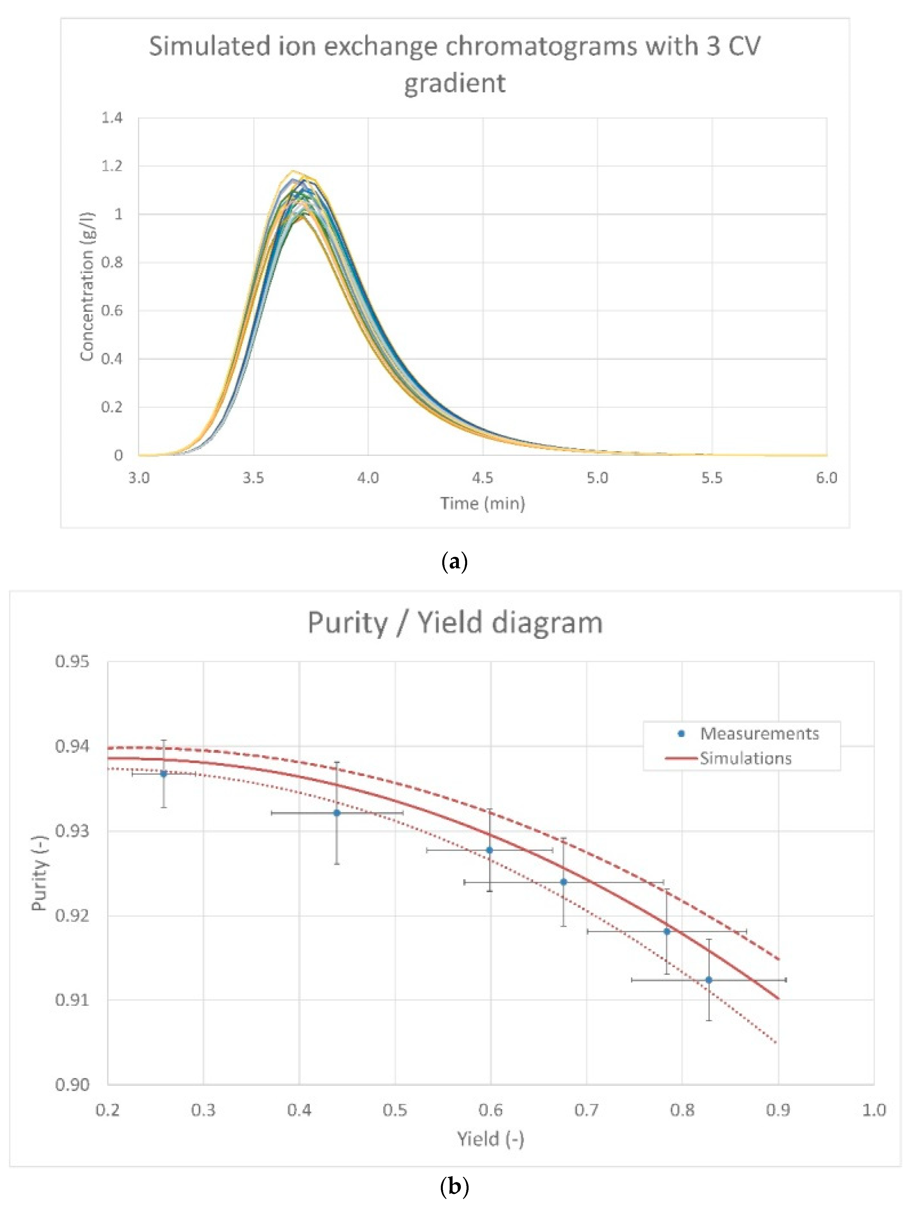
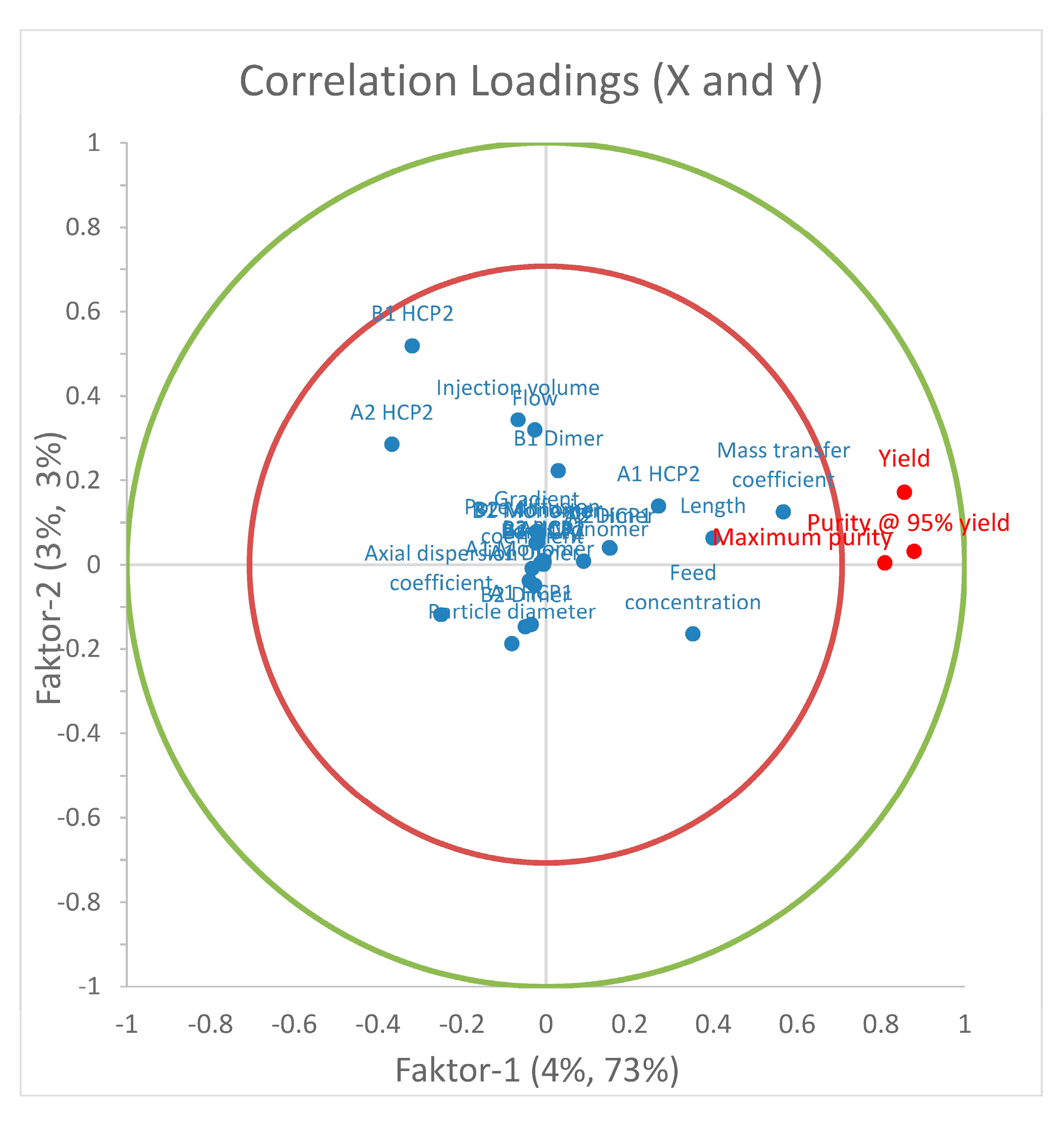
5.1. First Case Study: General Rate Model for Monoclonal Antibody Purification
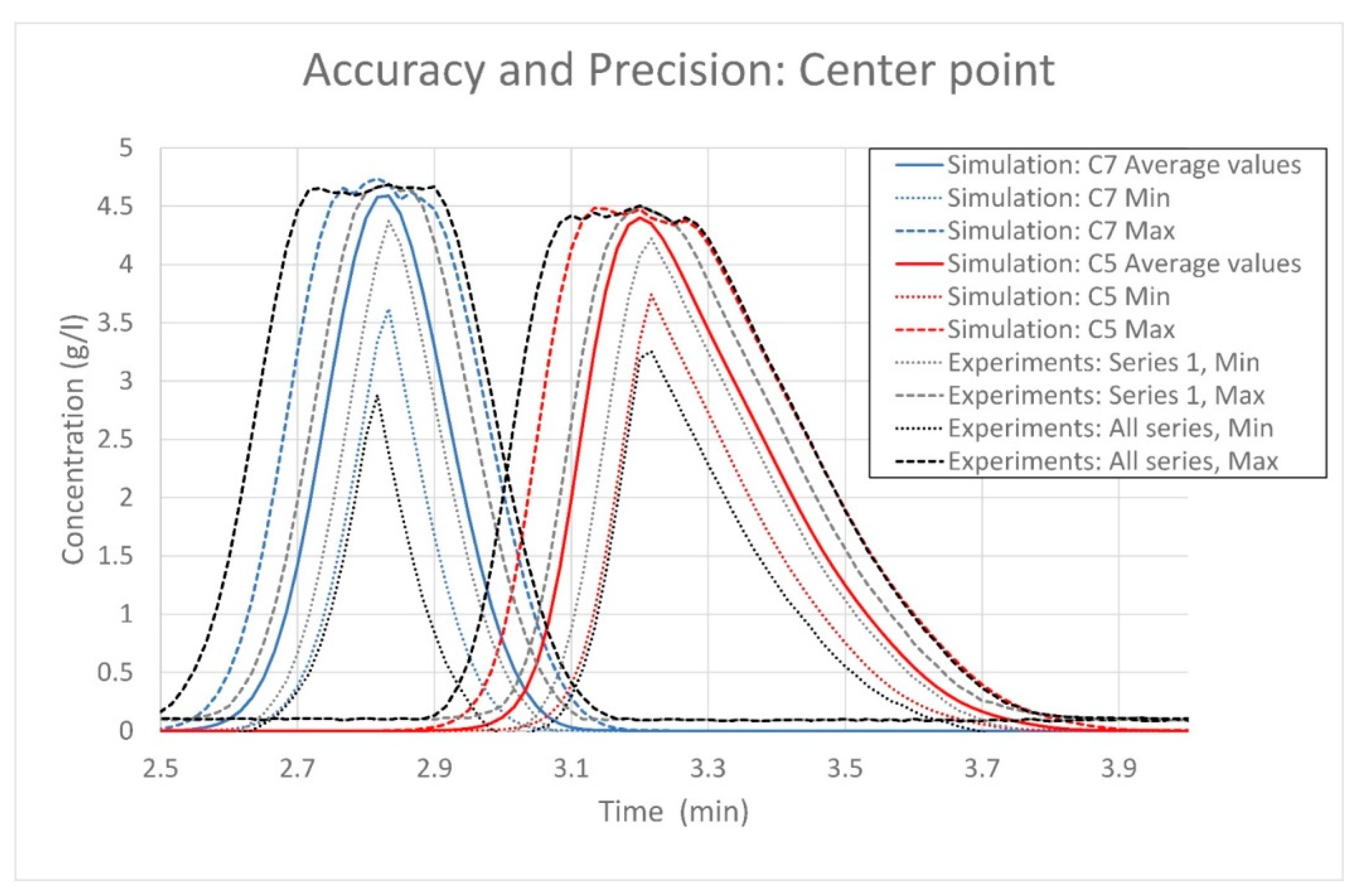
5.2. Second Case Study: Lumped Pore Diffusion Model for Continuous Chromatography of Cycloheptanone and Cyclopentanone
6. Discussion and Conclusions
Author Contributions
Funding
Acknowledgments
Conflicts of Interest
Abbreviations
| (-) | Parameter to calculate maximum loading in dependence of modifier concentration | |
| (g/L) | Parameter to calculate maximum loading in dependence of modifier concentration | |
| (L/mol) | Parameter to calculate Henry coefficient in dependence of modifier concentration | |
| (-) | Parameter to calculate Henry coefficient in dependence of modifier concentration | |
| C5 | Cyclopentanone | |
| C7 | Cycloheptanone | |
| CHO | Chinese Hamster Ovary (cells) | |
| (g/L) | Concentration of component i | |
| (g/L) | Concentration of component i inside the pores | |
| CV | Column volume | |
| (cm²/s) | Axial dispersion coefficient | |
| Deff | (cm²/s) | Effective diffusion coefficient |
| DoEs | Design-of-experiments | |
| (cm²/s) | Molecular diffusion coefficient | |
| (cm) | Particle diameter | |
| Dp,i | (cm²/s) | Pore diffusion coefficient |
| DS,i | (cm²/s) | Surface diffusion coefficient |
| (-) | Porosity | |
| (-) | Voidage | |
| Hi | (-) | Henry coefficient of component i |
| HCP | Host cell protein | |
| IgG | Immunoglobulin G | |
| Ki | (L/g) | Langmuir coefficient of component i |
| (cm/s) | Effective mass transport coefficient | |
| kf | (cm/s) | Mass transport coefficient |
| l | (cm) | Length |
| mAb | Monoclonal antibody | |
| PAT | Process Analytical Technology | |
| (-) | Peclet number | |
| PLS | Partial least squares (regression) | |
| qi | (g/L) | Loading of component i |
| QbD | Quality-by-design | |
| qmax,i | (g/L) | Maximum loading capacity of component i |
| r | (cm) | Radius |
| Re | (-) | Reynolds number |
| (cm) | Particle radius | |
| (-) | Sherwood number | |
| SEC | Size exclusion chromatography | |
| t | (s); (min) | Time |
| (s); (min) | Mean residence time | |
| (cm/s) | Interstitial velocity | |
| v | (cm/s) | Velocity |
| (mL/min) | Volumetric flow | |
| (mL) | Volume of column | |
| (mg/(cm × s)) | Dynamic viscosity | |
| (g/L) | Density | |
| (s²) | Variance | |
| (-) | Tortuosity parameter | |
| (-) | Hindrance coefficient |
References
- Strube, J. Technische Chromatographie: Auslegung, Optimierung, Betrieb und Wirtschaftlichkeit; Univ., Habil.-Schr.—Dortmund, 1999, Als Manuskript Gedruckt; Shaker: Aachen, Germany, 2000; ISBN 3826568974. [Google Scholar]
- Dünnebier, G.; Engell, S.; Klatt, K.-U.; Schmidt-Traub, H.; Strube, J.; Weirich, I. Modeling of simulated moving bed chromatographic processes with regard to process control design. Comput. Chem. Eng. 1998, 22, S855–S858. [Google Scholar] [CrossRef]
- Rodrigues, R.C.; Araújo, J.M.; Eusébio, M.F.; Mota, J.P. Experimental assessment of simulated moving bed and varicol processes using a single-column setup. J. Chromatogr. A 2007, 1142, 69–80. [Google Scholar] [CrossRef] [PubMed]
- Mota, J.P.B.; Araújo, J.M.M. Single-column simulated-moving-bed process with recycle lag. AIChE J. 2005, 51, 1641–1653. [Google Scholar] [CrossRef]
- Baur, D.; Angarita, M.; Müller-Späth, T.; Steinebach, F.; Morbidelli, M. Comparison of batch and continuous multi-column protein a capture processes by optimal design. Biotechnol. J. 2016, 11, 920–931. [Google Scholar] [CrossRef] [PubMed]
- Aumann, L.; Melter, L.; Ströhlein, G.; Morbidelli, M.; Müller-Späth, T. Chromatographic separation of three monoclonal antibody variants using multicolumn countercurrent solvent gradient purification (MCSGP). Biotechnol. Bioeng. 2008, 100, 1166–1177. [Google Scholar]
- International Council for Harmonisation of Technical Requirements for Pharmaceuticals for Human Use. Quality Risk Management Q9, 2005 (Step 4 Version). Available online: https://www.ich.org/fileadmin/Public_Web_Site/ICH_Products/Guidelines/Quality/Q9/Step4/Q9_Guideline.pdf (accessed on 17 January 2018).
- International Council for Harmonisation of Technical Requirements for Pharmaceuticals for Human Use. Pharmaceutical Quality System Q10, 2008 (Step 4 Version). Available online: Available online: http://www.ich.org/fileadmin/Public_Web_Site/ICH_Products/Guidelines/Quality/Q10/Step4/Q10_Guideline.pdf (accessed on 17 January 2018).
- International Council for Harmonisation of Technical Requirements for Pharmaceuticals for Human Use. Pharmaceutical Development Q8 (R2), 2009 (Step 4 Version). Available online: https://www.ich.org/fileadmin/Public_Web_Site/ICH_Products/Guidelines/Quality/Q8_R1/Step4/Q8_R2_Guideline.pdf (accessed on 2 January 2015).
- International Council for Harmonisation of Technical Requirements for Pharmaceuticals for Human Use. Development and Manufacturing of Drug Substances Q11, 2013 (Step 4 Version). Available online: http://www.ich.org/fileadmin/Public_Web_Site/ICH_Products/Guidelines/Quality/Q11/Q11_Step_4.pdf (accessed on 17 January 2018).
- Degerman, M.; Westerberg, K.; Nilsson, B. A Model-Based Approach to Determine the Design Space of Preparative Chromatography. Chem. Eng. Technol. 2009, 32, 1195–1202. [Google Scholar] [CrossRef]
- Del Val, I.J.; Kontoravdi, C.; Nagy, J.M. Towards the implementation of quality by design to the production of therapeutic monoclonal antibodies with desired glycosylation patterns. Biotechnol. Prog. 2010, 26, 1505–1527. [Google Scholar] [CrossRef]
- U.S. Food & Drug Administration. Guidance for Industry: Pharmacogenomic Data Submissions. Biotechnol. Law Rep. 2003, 23, 68–86. [Google Scholar] [CrossRef]
- U.S. Food & Drug Administration. Guidance for Industry—Sterile Drug Products Produced by Aseptic Processing—Current Good Manufacturing Practice; FDA: Rockville, MD, USA, 2004.
- U.S. Food & Drug Administration. Guidance for Industry PAT—A Framework for Innovative Pharmaceutical Development, Manufacturing, and Quality Assurance; FDA: Rockville, MD, USA, 2004.
- Peraman, R.; Bhadraya, K.; Reddy, Y.P. Analytical Quality by Design: A Tool for Regulatory Flexibility and Robust Analytics. Int. J. Anal. Chem. 2015, 2015, 868727. [Google Scholar] [CrossRef]
- Schmidt, A.; Strube, J. Distinct and Quantitative Validation Method for Predictive Process Modeling with Examples of Liquid-Liquid Extraction Processes of Complex Feed Mixtures. Processes 2019, 7, 298. [Google Scholar] [CrossRef]
- Guiochon, G.; Felinger, A.; Shirazi, D.G.; Katti, A.M. Fundamentals of Preparative and Nonlinear Chromatography, 2nd ed.; Elsevier Academic Press: Cambridge, MA, USA, 2006. [Google Scholar]
- Gu, T. Mathematical Modeling and Scale-Up of Liquid Chromatography; Springer International Publishing: Cham, Switzerland, 2015. [Google Scholar]
- Beltscheva, D. Linear two-step gradient counter-current chromatography Analysis based on a recursive solution of an equilibrium stage model. J. Chromatogr. A 2003, 989, 31–45. [Google Scholar] [CrossRef]
- Van Deemter, J.; Zuiderweg, F.; Klinkenberg, A. Longitudinal diffusion and resistance to mass transfer as causes of nonideality in chromatography. Chem. Eng. Sci. 1956, 5, 271–289. [Google Scholar] [CrossRef]
- Huuk, T.C.; Briskot, T.; Hahn, T.; Hubbuch, J. A versatile noninvasive method for adsorber quantification in batch and column chromatography based on the ionic capacity. Biotechnol. Prog. 2016, 32, 666–677. [Google Scholar] [CrossRef] [PubMed]
- Kumar, V.; Leweke, S.; Von Lieres, E.; Rathore, A.S. Mechanistic modeling of ion-exchange process chromatography of charge variants of monoclonal antibody products. J. Chromatogr. A 2015, 1426, 140–153. [Google Scholar] [CrossRef] [PubMed]
- Pirrung, S.M.; Van Der Wielen, L.A.M.; Van Beckhoven, R.F.W.C.; Van De Sandt, E.J.A.X.; Eppink, M.H.M.; Ottens, M. Optimization of biopharmaceutical downstream processes supported by mechanistic models and artificial neural networks. Biotechnol. Prog. 2017, 33, 696–707. [Google Scholar] [CrossRef] [PubMed]
- Shekhawat, L.K.; Chandak, M.; Rathore, A.S. Mechanistic modeling of hydrophobic interaction chromatography for monoclonal antibody purification: Process optimization in the quality by design paradigm. J. Chem. Technol. Biotechnol. 2017, 92, 2527–2537. [Google Scholar] [CrossRef]
- Wang, G.; Briskot, T.; Hahn, T.; Baumann, P.; Hubbuch, J. Root cause investigation of deviations in protein chromatography based on mechanistic models and artificial neural networks. J. Chromatogr. A 2017, 1515, 146–153. [Google Scholar] [CrossRef]
- Westerberg, K.; Broberg Hansen, E.; Degerman, M.; Budde Hansen, T.; Nilsson, B. Model-Based Process Challenge of an Industrial Ion-Exchange Chromatography Step. Chem. Eng. Technol. 2012, 35, 183–190. [Google Scholar] [CrossRef]
- Kucera, E. Contribution to the theory of chromatography: Linear non-equilibrium elution chromatography. J. Chromatogr. 1965, 19, 237–248. [Google Scholar] [CrossRef]
- Gu, T. Mathematical Modeling and Scale-up of Liquid Chromatography. In Mathematical Modeling and Scale-Up of Liquid Chromatography; Springer: Berlin/Heidelberg, Germany, 1995. [Google Scholar]
- Felinger, A.; Guiochon, G. Comparison of the Kinetic Models of Linear Chromatography. Chromatographia 2004, 60, S175–S180. [Google Scholar] [CrossRef]
- Zobel-Roos, S. Entwicklung, Modellierung und Validierung von Integrierten Kontinuierlichen Gegenstrom-Chromatographie-Prozessen, 1st ed.; Shaker: Düren, Germany, 2018; ISBN 3844061878. [Google Scholar]
- Juza, M. Development of an high-performance liquid chromatographic simulated moving bed separation from an industrial perspective. J. Chromatogr. A 1999, 865, 35–49. [Google Scholar] [CrossRef]
- Sixt, M.; Uhlenbrock, L.; Strube, J. Toward a Distinct and Quantitative Validation Method for Predictive Process Modelling—On the Example of Solid-Liquid Extraction Processes of Complex Plant Extracts. Processes 2018, 6, 66. [Google Scholar] [CrossRef]
- Sobol, I.M. Global sensitivity indices for nonlinear mathematical models and their Monte Carlo estimates. Math. Comput. Simul. 2001, 55, 271–280. [Google Scholar] [CrossRef]
- Saltelli, A.; Ratto, M.; Tarantola, S.; Campolongo, F. Update 1 of: Sensitivity Analysis for Chemical Models. Chem. Rev. 2012, 112, 1–21. [Google Scholar] [CrossRef] [PubMed]
- Lamboni, M.; Makowski, D.; Lehuger, S.; Gabrielle, B.; Monod, H. Multivariate global sensitivity analysis for dynamic crop models. Field Crop. Res. 2009, 113, 312–320. [Google Scholar] [CrossRef]
- Altenhöner, U.; Meurer, M.; Strube, J.; Schmidt-Traub, H. Parameter estimation for the simulation of liquid chromatography. J. Chromatogr. A 1997, 769, 59–69. [Google Scholar] [CrossRef]
- Kornecki, M.; Strube, J. Accelerating Biologics Manufacturing by Upstream Process Modelling. Processes 2019, 7, 166. [Google Scholar] [CrossRef]
- Kaczmarski, K.; Cavazzini, A.; Szabelski, P.; Zhou, D.; Liu, X.; Guiochon, G. Application of the general rate model and the generalized Maxwell–Stefan equation to the study of the mass transfer kinetics of a pair of enantiomers. J. Chromatogr. A 2002, 962, 57–67. [Google Scholar] [CrossRef]
- Kaczmarski, K.; Gubernak, M.; Zhou, D.; Guiochon, G. Application of the general rate model with the Maxwell–Stefan equations for the prediction of the band profiles of the 1-indanol enantiomers. Chem. Eng. Sci. 2003, 58, 2325–2338. [Google Scholar] [CrossRef]
- Piątkowski, W.; Antos, D.; Kaczmarski, K. Modeling of preparative chromatography processes with slow intraparticle mass transport kinetics. J. Chromatogr. A 2003, 988, 219–231. [Google Scholar] [CrossRef]
- Carta, G.; Jungbauer, A. Protein Chromatography: Process Development and Scale-Up; WILEY-VCH: Weinheim, Germany, 2010; ISBN 978-3-527-31819-3. [Google Scholar]
- Seidel-Morgenstern, A. Experimental determination of single solute and competitive adsorption isotherms. J. Chromatogr. A 2004, 1037, 255–272. [Google Scholar] [CrossRef] [PubMed]
- Asnin, L. Adsorption models in chiral chromatography. J. Chromatogr. A 2012, 1269, 3–25. [Google Scholar] [CrossRef] [PubMed]
- Blümel, C.; Kniep, H.; Seidel-Morgenstern, A. Measuring Adsorption Isotherms Using a Closed-Loop Perturbation Method to Minimize Sample Consumption. In Proceedings of the 6th International Conference of Fundamentals of Adsorption–FOA 6, Presqu’ile de Giens, France, 24–28 May 1998; Elsevier: Amsterdam, The Netherlands, 1998; pp. 449–454. [Google Scholar]
- Cavazzini, A.; Felinger, A.; Guiochon, G. Comparison between adsorption isotherm determination techniques and overloaded band profiles on four batches of monolithic columns. J. Chromatogr. A 2003, 1012, 139–149. [Google Scholar] [CrossRef]
- Ching, C.B.; Chu, K.H.; Ruthven, D.M. A study of multicomponent adsorption equilibria by liquid chromatography. AIChE J. 1990, 36, 275–281. [Google Scholar] [CrossRef]
- Gamba, G.; Rota, R.; Storti, G.; Carra, S.; Morbidelli, M. Absorbed solution theory models for multicomponent adsorption equilibria. AIChE J. 1989, 35, 959–966. [Google Scholar] [CrossRef]
- Hu, X.; Do, D.D. Comparing various multicomponent adsorption equilibrium models. AIChE J. 1995, 41, 1585–1592. [Google Scholar] [CrossRef]
- Heinonen, J.; Landa, H.O.R.; Sainio, T.; Seidel-Morgenstern, A. Use of Adsorbed Solution theory to model competitive and co-operative sorption on elastic ion exchange resins. Sep. Purif. Technol. 2012, 95, 235–247. [Google Scholar] [CrossRef]
- Emerton, D.A. Profitability in the Biosimilars Market: Can You Translate Scientific Excellence into a Healthy Commercial Return? BioProcess Int. 2013, 11, 6–23. [Google Scholar]
- Erto, A.; Lancia, A.; Musmarra, D. A modelling analysis of PCE/TCE mixture adsorption based on Ideal Adsorbed Solution Theory. Sep. Purif. Technol. 2011, 80, 140–147. [Google Scholar] [CrossRef]
- Myers, A.L.; Prausnitz, J.M. Thermodynamics of mixed-gas adsorption. AIChE J. 1965, 11, 121–127. [Google Scholar] [CrossRef]
- Costa, E.; Calleja, G.; Marrón, C.; Jiménez, A.; Pau, J. Equilibrium adsorption of methane, ethane, ethylene, and propylene and their mixtures on activated carbon. J. Chem. Eng. Data 1989, 34, 156–160. [Google Scholar] [CrossRef]
- Brooks, C.A.; Cramer, S.M. Steric mass-action ion exchange: Displacement profiles and induced salt gradients. AIChE J. 1992, 38, 1969–1978. [Google Scholar] [CrossRef]
- Langmuir, I. The adsorption of gases on plane surfaces of glass, mica and platinum. J. Am. Chem. Soc. 1918, 40, 1361–1403. [Google Scholar] [CrossRef]
- Gronemeyer, P.; Strube, J. Entwicklung einer Methode zur Integration von Upstream und Downstream Processing am Beispiel der Herstellung monoklonaler Antikörper. Ph.D. Thesis, Technische Universität Clausthal, Clausthal-Zellerfeld, Germany, 2017. [Google Scholar]
- Zobel-Roos, S.; Mouellef, M.; Siemers, C.; Strube, J. Process Analytical Approach towards Quality Controlled Process Automation for the Downstream of Protein Mixtures by Inline Concentration Measurements Based on Ultraviolet/Visible Light (UV/VIS) Spectral Analysis. Antibodies 2017, 6, 24. [Google Scholar] [CrossRef]
- Dephillips, P.; Lenhoff, A.M. Pore size distributions of cation-exchange adsorbents determined by inverse size-exclusion chromatography. J. Chromatogr. A 2000, 883, 39–54. [Google Scholar] [CrossRef]
- Goto, M.; McCoy, B.J. Inverse size-exclusion chromatography for distributed pore and solute sizes. Chem. Eng. Sci. 2000, 55, 723–732. [Google Scholar] [CrossRef]
- Levenspiel, O. Chemical Reaction Engineering, 3rd ed.; Wiley: New York, NY, USA, 1999; ISBN 9780471254249. [Google Scholar]
- Chung, S.F.; Wen, C.Y. Longitudinal dispersion of liquid flowing through fixed and fluidized beds. AIChE J. 1968, 14, 857–866. [Google Scholar] [CrossRef]
- Dwivedi, P.N.; Upadhyay, S.N. Particle-Fluid Mass Transfer in Fixed and Fluidized Beds. Ind. Eng. Chem. Process. Des. Dev. 1977, 16, 157–165. [Google Scholar] [CrossRef]
- Williamson, J.E.; Bazaire, K.E.; Geankoplis, C.J. Liquid-Phase Mass Transfer at Low Reynolds Numbers. Ind. Eng. Chem. Fundam. 1963, 2, 126–129. [Google Scholar] [CrossRef]
- Wilson, E.J.; Geankoplis, C.J. Liquid Mass Transfer at Very Low Reynolds Numbers in Packed Beds. Ind. Eng. Chem. Fundam. 1966, 5, 9–14. [Google Scholar] [CrossRef]
- Forrer, N. Antibody Purification with Ion-Exchange Chromatography Dissertation; Eidgenössische Technische Hochschule: Zürich, Switzerland, 2008. [Google Scholar]
- Young, M.E.; Carroad, P.A.; Bell, R.L. Estimation of diffusion coefficients of proteins. Biotechnol. Bioeng. 1980, 22, 947–955. [Google Scholar] [CrossRef]
- McCoy, M.; Kalghatgi, K.; Regnier, F.E.; Afeyan, N. Perfusion chromatography—Characterization of column packings for chromatography of proteins. J. Chromatogr. A 1996, 743, 221–229. [Google Scholar] [CrossRef]
- Samuelsson, J.; Arnell, R.; Fornstedt, T. Potential of adsorption isotherm measurements for closer elucidating of binding in chiral liquid chromatographic phase systems. J. Sep. Sci. 2009, 32, 1491–1506. [Google Scholar] [CrossRef] [PubMed]
- Ahuja, S. (Ed.) Handbook of Bioseparations; Academic Press: San Diego, CA, USA, 2000; ISBN 9780080507798. [Google Scholar]
- Camperi, S.A.; del Cañizo, A.A.; Wolman, F.J.; Smolko, E.E.; Cascone, O.; Grasselli, M. Protein adsorption onto tentacle cation-exchange hollow-fiber membranes. Biotechnol. Prog. 1999, 15, 500–505. [Google Scholar] [CrossRef] [PubMed]
- Desta, M.B. Batch Sorption Experiments: Langmuir and Freundlich Isotherm Studies for the Adsorption of Textile Metal Ions onto Teff Straw (Eragrostis tef) Agricultural Waste. J. Thermodyn. 2013, 2013, 1–6. [Google Scholar] [CrossRef]
- Lan, Q.; Bassi, A.S.; Zhu, J.X.; Margaritis, A. A modified Langmuir model for the prediction of the effects of ionic strength on the equilibrium characteristics of protein adsorption onto ion exchange/affinity adsorbents. Chem. Eng. J. 2001, 81, 179–186. [Google Scholar] [CrossRef]
- Dose, E.V.; Jacobson, S.; Guiochon, G. Determination of isotherms from chromatographic peak shapes. Anal. Chem. 2002, 63, 833–839. [Google Scholar] [CrossRef]
- Felinger, A.; Cavazzini, A.; Guiochon, G. Numerical determination of the competitive isotherm of enantiomers. J. Chromatogr. A 2003, 986, 207–225. [Google Scholar] [CrossRef]
- Jönsson, J.Å.; Lökvist, P. Determination of adsorption isotherms from chromatographic measurements, using the peak maxima method. J. Chromatogr. A 1987, 408, 1–7. [Google Scholar]
- Jacobson, J.M.; Frenz, J.H.; Horvath, C.G. Measurement of competitive adsorption isotherms by frontal chromatography. Ind. Eng. Chem. Res. 1987, 26, 43–50. [Google Scholar] [CrossRef]
- Helfferich, F. Travel of molecules and disturbances in chromatographic columns: A paradox and its resolution. J. Chem. Educ. 1964, 41, 410. [Google Scholar] [CrossRef]
- Mihlbachler, K.; Kaczmarski, K.; Seidel-Morgenstern, A.; Guiochon, G. Measurement and modeling of the equilibrium behavior of the Tröger’s base enantiomers on an amylose-based chiral stationary phase. J. Chromatogr. A 2002, 955, 35–52. [Google Scholar] [CrossRef]
- Muralidharan, P.K.; Ching, C.B. Determination of Multicomponent Adsorption Equilibria by Liquid Chromatography. Ind. Eng. Chem. Res. 1997, 36, 407–413. [Google Scholar] [CrossRef]
- Chen, T.-W.; Pinto, N.G.; Van Brocklin, L. Rapid method for determining multicomponent Langmuir parameters for displacement chromatography. J. Chromatogr. A 1989, 484, 167–185. [Google Scholar] [CrossRef]
- Helfferich, F.G. The h-and ω-transformations in multicomponent fixed-bed ion exchange and adsorption: Equivalent mathematics, different scope. Chem. Eng. Sci. 1991, 46, 3320–3323. [Google Scholar] [CrossRef]
- Jen, S.; Pinto, N.G. Modification of the h-root method for the determination of multicomponent Langmuir coefficients in liquid chromatography. J. Chromatogr. A 1994, 662, 396–400. [Google Scholar] [CrossRef]
- Lapizco-Encinas, B.H.; Pinto, N.G. Determination of adsorption isotherms of proteins by H-root method: Comparison between open micro-channels and conventional packed columns. J. Chromatogr. A 2005, 1070, 201–205. [Google Scholar] [CrossRef]
- Zobel-Roos, S.; Thiess, H.; Gronemeyer, P.; Ditz, R.; Strube, J.; Zobel-Roos, S.; Subramanian, G. Continuous Chromatography as a Fully Integrated Process in Continuous Biomanufacturing. In Continuous Biomanufacturing—Innovative Technologies and Methods; Wiley: Hoboken, NJ, USA, 2017; pp. 369–392. [Google Scholar]
- Zobel-Roos, S.; Stein, D.; Strube, J. Evaluation of Continuous Membrane Chromatography Concepts with an Enhanced Process Simulation Approach. Antibodies 2018, 7, 13. [Google Scholar] [CrossRef]
- Wiesel, A.; Schmidt-Traub, H.; Lenz, J.; Strube, J. Modelling gradient elution of bioactive multicomponent systems in non-linear ion-exchange chromatography. J. Chromatogr. A 2003, 1006, 101–120. [Google Scholar] [CrossRef]
- Helling, C.; Strube, J. Modeling and Experimental Model Parameter Determination with Quality by Design for Bioprocesses. Biopharm. Prod. Technol. 2012, 1, 409–443. [Google Scholar]
- Zobel, S.; Helling, C.; Ditz, R.; Strube, J. Design and Operation of Continuous Countercurrent Chromatography in Biotechnological Production. Ind. Eng. Chem. Res. 2014, 53, 9169–9185. [Google Scholar] [CrossRef]
- Kornecki, M.; Mestmäcker, F.; Zobel-Roos, S.; De Figueiredo, L.H.; Schlüter, H.; Strube, J. Host Cell Proteins in Biologics Manufacturing: The Good, the Bad, and the Ugly. Antibodies 2017, 6, 13. [Google Scholar] [CrossRef]
- Gottschalk, U. Process Scale Purification of Antibodies, 2nd ed.; Gottschalk, U., Ed.; John Wiley & Sons Inc.: Hoboken, NJ, USA, 2017; ISBN 9781119126935. [Google Scholar]
- Brestrich, N.; Briskot, T.; Osberghaus, A.; Hubbuch, J. A tool for selective inline quantification of co-eluting proteins in chromatography using spectral analysis and partial least squares regression. Biotechnol. Bioeng. 2014, 111, 1365–1373. [Google Scholar] [CrossRef] [PubMed]


| Process Parameters | Design Range | Unit | Purity IgG | Yield IgG | Rationale |
|---|---|---|---|---|---|
| Temperature | 15 to 25 | °C | No | No | No impact in this range, thus not included in this study. |
| Length | 5 to 15 | cm | Low | Low | Reasonable range for potential use in small-scale batch purifications or continuous chromatography. |
| Diameter | 1 | cm | No | No | The diameter itself is of less importance. Resulting velocity changes are represented with flow changes. |
| Flow | 1.5 to 2.5 | mL/min | Low | Low | Reasonable range for this column dimensions and for the use in preparative chromatography. |
| Gradient | 3 to 7 | CV | High | High | In continuous chromatography (e.g., iCCC (integrated CounterCurrent Chromatography) or MCSGP (Multicolumn Countercurrent Solvent Gradient Purification)), quality/yield trade-off is avoided. Speed beats batch separation performance. |
| Feed concentration | 4.2 to 5.6 | g/L | Low | Low | Feed variation results from upstream batch variation. |
| Injection volume | 25 to 75 | µL | Low | Low | |
| Total porosity | 0.93 to 0.97 | - | Medium | Medium | When the stationary phase is already chosen, than the variation in said parameters should be low. Reasons for variation might be, for example, packing quality, swelling due to salt concentration, or batch variations in adsorber material production. |
| Particle diameter | 20 to 40 | µm | Medium | Medium | |
| Axial dispersion coefficient | 0.0005 to 0.005 | cm²/s | Medium | Medium | |
| Mass transfer coefficient | 0.0002 to 0.02 | 1/s | Medium | Medium | |
| Pore diffusion coefficient | 1.3 × 10⁻⁸ to 1.3 × 10⁻⁶ | cm²/s | Medium | Medium | |
| Isotherm parameters | 3% variation | - | High | High | Isotherm parameters underlie diversified influences (e.g., adsorber material or eluent composition). |
| Factor | Unit | Mean Value | Error | Source | |
|---|---|---|---|---|---|
| Absolute | Relative | ||||
| Length | cm | 5 | ±0.025 | ±0.5% | Data sheet |
| Flow | mL/min | 0.5 | ±0.01 | ±2.0% | Data sheet |
| Feed concentration | g/L | 4.8 | ±0.6 | ±12.5% | Repeatability (DF) |
| Injection volume | µL | 99 | ±2 | ±2% | Data sheet |
| Total porosity | - | 0.95 | ±0.001 | ±0.11% | Repeatability |
| Particle diameter | µm | 30 | 0 | 0% | Same column |
| Axial dispersion coefficient | cm²/s | 2.75 × 10⁻³ | 0 | 0% | Correlation |
| Mass transport coefficient | 1/s | 2.0 × 10⁻³ | 0 | 0% | Correlation |
| Pore diffusion coefficient | cm²/s | 1.3 × 10⁻⁷ | 0 | 0% | Correlation |
| Gradient | CV | 5 | ±0.1 | ±2.0% | Data sheet |
| Isotherm parameter | All assumed with ±3% | ||||
| Process Outputs: | Product Quality | Process Performance | Rationale | ||||
|---|---|---|---|---|---|---|---|
| Process Parameters | Design Range | Unit | Purity C7 | Purity C5 | Yield C7 | Yield C5 | |
| Temperature | 15 to 25 | °C | No | No | No | No | No impact in this range, thus not included in this study. |
| Length | 5 to 15 | cm | High | High | High | High | Reasonable range for potential use in continuous, especially simulated moving-bed chromatography. |
| Diameter | - | cm | No | No | No | No | The diameter itself is of less importance. Resulting velocity changes are represented with flow changes. |
| Flow | 10 to 15 | mL/min | Medium | Medium | Low | Low | Reasonable range for this column dimensions and for the use in preparative chromatography. |
| Eluent composition | - | - | No | No | No | No | Eluent composition has impact on the isotherms, thus is included in isotherm parameter variation. |
| Feed concentration | 50 to 75 | g/L | Low | Low | Low | Low | In this case study, combined feed concentration and injection volume are relatively low, thus the impact should be low, although this might be completely different for other separations. |
| Injection volume | 50 to 150 | µL | Low | Low | Low | Low | |
| Total porosity | 0.812 to 0.898 | - | Medium | Medium | Medium | Medium | When the stationary phase is already chosen, than the variation in said parameters should be low. Reasons for variation might be, for example, packing quality or batch variations in adsorber material production. |
| Particle diameter | 18 to 22 | µm | Medium | Medium | Medium | Medium | |
| Axial dispersion coefficient | 0.0007 to 0.00013 | cm²/s | Medium | Medium | Medium | Medium | |
| Mass transport coefficient | 0.007 to 0.013 | 1/s | Medium | Medium | Medium | Medium | |
| Henry coefficient C7 | 5.5 to 7.5 | - | High | High | High | High | Isotherm parameters underlie diversified influences, for example, adsorber material or eluent composition. |
| Henry coefficient C5 | 8 to 10 | - | High | High | High | High | |
| Langmuir coefficient C7 | 0.0041 to 0.0076 | L/g | High | High | High | High | |
| Langmuir coefficient C5 | 0.035 to 0.066 | L/g | High | High | High | High | |
| Parameter | Unit | Mean Value | Error | Origin | |
|---|---|---|---|---|---|
| Absolute | Relative | ||||
| Flow | mL/min | 12.5 | ±1.25 | ±2% | Data sheet |
| Length | cm | 10 | No change, only one column used | ||
| Diameter | cm | 1.6 | No change, only one column used | ||
| Feed concentration | g/L | 62.5 | ±1.25 | ±2% | HPLC Analysis |
| Voidage | - | 0.855 | ±0.0009 | ±0.1% | Reproducibility |
| Axial dispersion coefficient | cm²/s | 1 × 10⁻⁴ | ±5 × 10⁻⁶ | ±5% | Error propagation |
| Mass transfer coefficient | 1/s | 1 × 10⁻² | ±5 × 10⁻⁴ | ±5% | Error propagation |
| Henry coefficient C7 | - | 6.58 | ±0.2 | ±3% | Error propagation |
| Langmuir coefficient C7 | L/g | 5.8 × 10⁻³ | ±1.8 × 10⁻⁴ | ±3% | Error propagation |
| Henry coefficient C5 | - | 9.0 | ±0.27 | ±3% | Error propagation |
| Langmuir coefficient C5 | L/g | 5.1 × 10⁻² | ±1.5 × 10⁻³ | ±3% | Error propagation |
© 2019 by the authors. Licensee MDPI, Basel, Switzerland. This article is an open access article distributed under the terms and conditions of the Creative Commons Attribution (CC BY) license (http://creativecommons.org/licenses/by/4.0/).
Share and Cite
Zobel-Roos, S.; Mouellef, M.; Ditz, R.; Strube, J. Distinct and Quantitative Validation Method for Predictive Process Modelling in Preparative Chromatography of Synthetic and Bio-Based Feed Mixtures Following a Quality-by-Design (QbD) Approach. Processes 2019, 7, 580. https://0-doi-org.brum.beds.ac.uk/10.3390/pr7090580
Zobel-Roos S, Mouellef M, Ditz R, Strube J. Distinct and Quantitative Validation Method for Predictive Process Modelling in Preparative Chromatography of Synthetic and Bio-Based Feed Mixtures Following a Quality-by-Design (QbD) Approach. Processes. 2019; 7(9):580. https://0-doi-org.brum.beds.ac.uk/10.3390/pr7090580
Chicago/Turabian StyleZobel-Roos, Steffen, Mourad Mouellef, Reinhard Ditz, and Jochen Strube. 2019. "Distinct and Quantitative Validation Method for Predictive Process Modelling in Preparative Chromatography of Synthetic and Bio-Based Feed Mixtures Following a Quality-by-Design (QbD) Approach" Processes 7, no. 9: 580. https://0-doi-org.brum.beds.ac.uk/10.3390/pr7090580