A Retrofit Hierarchical Architecture for Real-Time Optimization and Control Integration


1
State Key Laboratory of Industrial Control Technology, Institute of Cyber-Systems and Control, Zhejiang University, Yuquan Campus, Hangzhou 310027, China
2
Department of Chemical Engineering, Queen’s University, 19 Division St., Kingston, ON K7L 3N6, Canada
*
Author to whom correspondence should be addressed.
Processes 2020, 8(2), 181; https://0-doi-org.brum.beds.ac.uk/10.3390/pr8020181
Submission received: 9 December 2019
/
Revised: 25 January 2020
/
Accepted: 29 January 2020
/
Published: 5 February 2020
(This article belongs to the Special Issue Process Optimization and Control)
Abstract
:To achieve the optimal operation of chemical processes in the presence of disturbances and uncertainty, a retrofit hierarchical architecture (HA) integrating real-time optimization (RTO) and control was proposed. The proposed architecture features two main components. The first is a fast extremum-seeking control (ESC) approach using transient measurements that is employed in the upper RTO layer. The fast ESC approach can effectively suppress the impact of plant-model mismatch and steady-state wait time. The second is a global self-optimizing control (SOC) scheme that is introduced to integrate the RTO and control layers. The proposed SOC scheme minimizes the global average loss based on the approximation of necessary conditions of optimality (NCO) over the entire operating region. A least-squares regression technique was adopted to select the controlled variables (CVs) as linear combinations of measurements. The proposed method does not require the second order derivative information, therefore, it is numerically more reliable and robust. An exothermic reaction process is presented to illustrate the effectiveness of the proposed method.
1. Introduction
The effectiveness of optimal operation has been widely recognized, and becomes more important when considering environmental impact and market competition in the chemical industry [1,2]. The hierarchical architecture (HA) of chemical processes includes the real-time optimization (RTO) layer and the control layer, which operate on different time scales and have different tasks, respectively [3,4]. In the RTO layer, daily operation has been optimized based on a steady-state process model. This layer is usually also divided into a site-wide optimization layer and local optimization layer. The control layer is located below the RTO layer and it aims to ensure system stability, reject various disturbances, and maintain the controlled variables (CVs) at the desired set-points. This layer can be further divided into a supervisory control layer and a regulatory control layer. The objective of the supervisory control layer is to satisfy the operational constraints, e.g., those configured within multivariable model predictive controllers (MPC), whereas the objective of the regulatory control layer is to stabilize the actual plant with proportional integral-derivative (PID) controllers. These layers are connected through different set-points, which are passed from the higher layers to the lower layers.
The performance of the chemical processes tends to decay with time under various uncertainties and disturbances (e.g., equipment damage, raw material fluctuation, daily weather fluctuation and market demand change). Once such uncertainties or disturbances exist, the current operating strategy is no longer optimal. Thus, determining how to make better use of resources and energy to achieve optimal operation has become an important issue in the chemical industry. Depending on how this is realized, the approaches for achieving optimal operation of chemical processes can be classified into three categories, namely, the model-free approach, the online model-based approach and the offline model-based approach.
For the model-free approach, several measurement-based methods have been developed that avoid using an explicit process model. Necessary conditions of optimality (NCO) tracking [5], hill-climbing control [6] and extremum-seeking control (ESC) [7] belong in this category. These approaches use the input excitation to estimate the steady-state gradient from the cost measurement without the need for rigorous process models. Consequently, the advantage is that they can handle plant-model mismatch and unexpected disturbances. Nonetheless, these approaches need to wait for the process to settle down and reach a new steady state before estimating the gradient, therefore the convergence rate is slow. The concept of ESC is relatively old and can be traced back almost 100 years [8]. It has recently gained increased attention since the stability problem was proven by Krstic and Wang [9]. In recent years, there has been several advancements in ESC approaches such as the least-square-based ESC [10,11], discrete-time ESC [12], sliding-mode ESC [13], Newton-based ESC [14], etc. A common step included in all of these approaches is to drive the estimated steady-state gradient to zero under some specific control law.
The online model-based approach relies on measurements collected online together with the process model. Depending on the type of optimization problem, the online model-based approach can be further classified as steady-state real-time optimization (SRTO) [15] and dynamic real-time optimization (DRTO) [16] or economic model predictive control (EMPC) [17]. Due to the steady-state wait time for SRTO and computation complexity of DRTO and EMPC, the convergence rate for the online model-based approach is also slow. SRTO requires several preprocessing steps, such as steady-state detection, data reconciliation, parameter estimation and model adaptation before it can be used. A major improvement can be obtained in the data reconciliation step [18]. Recently, DRTO and EMPC have become more attractive due to their better performance in handling input and output constraints in comparison with SRTO. Both DRTO and EMPC use the dynamic model to predict future optimal input trajectories.
Of all of the offline model-based approaches, self-optimizing control (SOC) has been demonstrated to be the most attractive one. The concept of SOC was first proposed by Skogestad [4] to design the control structure. A set of offline selected CVs are said to be self-optimizing if by keeping them at constant set-points through a simple feedback control, the process operation automatically approaches optimum despite disturbances and uncertainties. In the past two decades, various methods of SOC have been reported. Instead of using individual measurements as CVs [19], using linear combinations of measurements as CVs has been proved to result in better performance [20]. Alstad [21] devised a null space method to select the linear combinations of measurements to achieve optimal operation around the nominal point. This method evolved into an extended null space method [22] to reduce the impact of implementation error. Meanwhile, Kariwala proposed an eigenvalue decomposition-based SOC method to minimize the local average loss and the local worst-case loss [23,24]. On this basis, a series of branch and bound-based methods were developed to fast screen the CV candidates [25,26,27,28]. A mixed-integer quadratic programming method was also proposed for measurements subset selection [29]. These methods are all based on linearized models around nominal operating points and thus they are only locally valid. More recently, the local SOC method has been advanced to the global method, which is based on the simulation data over the entire operating space. Some artificial intelligence techniques are also employed for the global SOC method [30,31]. For more detailed information about the SOC method, readers are referred to an overview of the state-of-the-art and open issues in the development of SOC by Jaschke [32].
The hierarchical architecture (HA) incorporating the SOC scheme has been reported in the literature. For example, Jaschke [33] presented a novel control hierarchy to combine the NCO tracking and the local SOC. The NCO tracking approach uses finite difference to periodically update the set-points to reduce the economic loss. Ye [34] developed a controlled variable adaptation-based structure to improve the optimizing performance. A two-layer control architecture integrating the SOC and modifier adaptation (MA) was also provided by Ye [35] to address the plant-model mismatch.
The main contribution of this work is a retrofit hierarchical architecture (HA) for integrating real-time optimization and control. Specifically, a fast extremum-seeking control (ESC) approach using transient measurements is employed in the upper RTO layer and the set-points are updated by driving the estimated steady-state gradient of the cost to zero. The ESC approach can effectively suppress the impact of the plant-model mismatch and steady-state wait time. The lower control layer is configured with a global SOC scheme to select the appropriate CVs and track the set-points delivered from the upper ESC layer. The SOC scheme minimizes the average loss globally and provides a faster reaction to expected disturbances. The proposed methodology inherits the advantages of both the fast ESC approach and the global SOC scheme.
The rest of this paper is arranged as follows: Section 2 introduces a fast extremum-seeking control (ESC) approach using transient measurements. Section 3 presents the concept of a global self-optimizing control (SOC) for CV selection. Section 4 devises a retrofit hierarchal architecture (HA) integrating real-time optimization (RTO) and control. An exothermic reaction process is used to investigate the advantages of the proposed methodologies in Section 5. Finally, the conclusions are summarized in Section 6.
2. Fast ESC Using Transient Measurements
The objective of the ESC scheme is to estimate the gradient of the cost function and drive it to zero under a specified control law (usually simple integral action). It can handle the plant-model mismatch or any other unexpected disturbances since it is a model-free adaptive control approach. The performance of this approach depends purely on the accuracy of the gradient estimation. Nevertheless, the drawbacks of this approach are that the convergence rate is slow and the cost function value is required. Hence, it fits better in the upper RTO layer.
An excitation signal (e.g., the sinusoidal signal or pseudo-random binary sequence signal) is commonly added to provide sufficient excitation for the gradient estimation in the ESC scheme. However, it requires a clear time scale separation between the process dynamics, excitation signal and convergence to the optimum [9]. Typically, the excitation signal that is chosen is 10 times slower than the plant dynamics such that the plant behaves like a static map. Furthermore, the selected integral gain is usually small enough such that the convergence to the optimum is another 10 times slower than the excitation signal, which means the overall convergence rate is about 100 times slower than the plant dynamics. This is unacceptable and impractical for real-time optimization of most processes. In order to address the steady-state wait time, which is caused by the local linear static map assumption, an alternative solution is to explicitly include the plant dynamics in the ESC approach. In this section, we introduce a fast ESC approach using transient measurements to significantly improve the convergence rate.
A local linear dynamic model, the auto regression exogenous (ARX) model was used as an effective way to include the plant dynamics. In the meantime, incorporating the plant dynamics in the gradient estimation removes the static map assumption, therefore, one does not need the time scale separation between the plant dynamics and the excitation signal. This results in a significantly faster convergence rate compared to the conventional ESC approach, which is also shown in the simulation results in Section 5.
For simplicity of derivation, we considered a nonlinear single input single output process, where the objective is to drive the cost Q to its optimal value by adjusting the input u.
The following assumptions should be met.
Assumption 1.
The plant cost Q can be measured or calculated.
Assumption 2.
The process can be represented as a combination of a nonlinear time invariant part and a linear stable time invariant dynamic part.
Assumption 3.
The nonlinear time invariant part is sufficiently smooth and continuously differentiable such that it has a unique optimal solution.
Assumption 4.
The set of active constraints do not change with disturbances and they are perfectly controlled.
One can use the transient measurements to estimate the gradient from the cost. A sliding window strategy containing the last N samples of data is used to fit the following ARX model:
where t denotes the current time, denotes the white noise signal, and denotes the order of the ARX model. The last N transient measurements of data are used to estimate the ARX parameters based on the linear least-squares method:
where represents the vector of the last (Nn) cost data, which is given by
and represents the characteristic vector, which is given by
where .
The analytical solution of problem (2) is given by
Introducing the notation, and where denotes the unit shift operator. Once the ARX parameters are estimated, a local linear dynamic model can be obtained in the form:
The steady-state gradient around the current operating point can then be estimated by
where the notation “^” means the estimated value, once is estimated, a simple integral controller can be used to drive the gradient to zero and update the controlled input. In discrete time, this can be expressed as
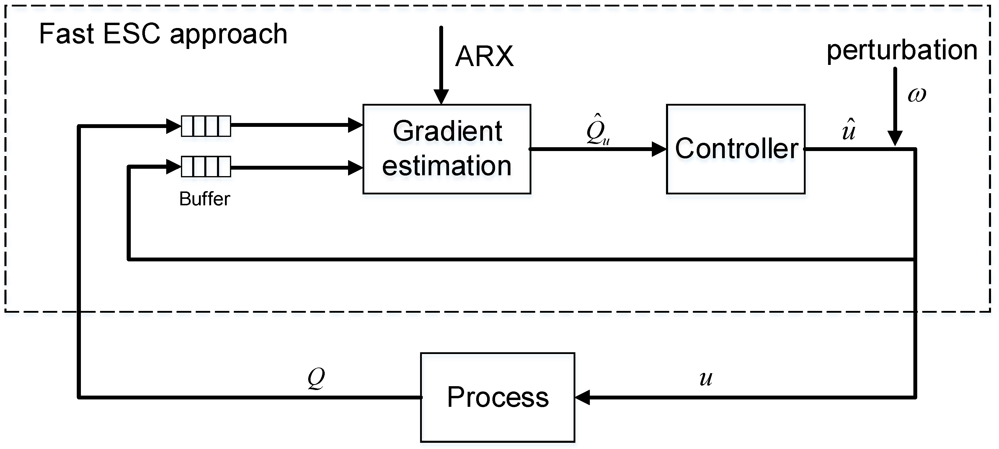
where denotes the integral gain and denotes the sample time. It is also necessary to add the perturbation signal (e.g., pseudo-random binary sequence signal) to the input for sufficient excitation, which yields The block diagram of the fast ESC approach is shown in Figure 1. The buffers are used to store the last N transient measurements of data.
In this section, a fast ESC approach was proposed using transient measurements, which is based on identifying a local linear ARX model around the current operating point. The steady-state gradient can be estimated from the identified ARX model. By using transient measurements, one can effectively eliminate the time scale separation between the plant dynamics and the excitation signal. This results in a significantly faster convergence rate compared to the classical ESC approach, which is also shown in the simulation results in Section 5. Additionally, the proposed approach can be extended to a multivariable system where each input should have a particular excitation signal to estimate the gradient, and the controller is a simple decentralized integral control framework.
3. Global SOC for CVs Selection
3.1. Basic Concept of SOC
The concept of SOC was first proposed to design control structures by selecting the appropriate measurement combination as the CVs. A set of offline selected CVs are said to be self-optimizing if by keeping them at constant set-points through a simple feedback control, the process operation automatically approaches optimum despite disturbances and uncertainties. Usually, the model-based approach has better convergence than the model-free approach, thus it fits better to integrate the RTO and control layers. Consider the following steady-state optimization problems:
where denotes the scalar cost function, denotes the manipulate variables (MVs), denotes the disturbance variables, denotes the theoretical measurements, which are calculated from the steady-state measurement model , denotes the constraints corresponding to the operating limits and product qualities (e.g., temperature limit, flow limit and product concentrations, etc.).
For the SOC method, the controlled variables (CVs) are selected as
where (with ) are the selected CVs, represents the selection matrix and denotes the available measurements, which are corrupted by the measurement noise . The steady-state measurement model is linearized around the nominal point as follows:
where denotes the steady-state gain matrix of with respect to and denotes the steady-state gain matrix of with respect to . Then, the loss function is defined as
where and denote the optimal cost function value and the optimal manipulated variables for a given disturbance , respectively. The ultimate goal is to keep the CVs at their desired set-points delivered from the upper layer by adjusting MVs . Meanwhile, the loss function for the expected disturbance and measurement noise is minimized.
For the SOC method [21,29], the CVs selection problem can be converted to minimize the average loss in the form of selection matrix as
where is the augmented matrix and denotes the Frobenius norm, and represent the diagonal matrices with the expected magnitudes of the disturbance and the measurement noise, respectively. represents the optimal sensitive matrix, denotes the Hessian matrix of with respect to .
The analytical solution to problem (13) can be derived:
It should be noted that the above results are derived on the basis of linearization around the nominal optimal point, therefore this method is only locally valid around the nominal optimal point. It may lead to large steady-state loss if the process moves far away from the nominal condition in the presence of various disturbances and uncertainties. Over time, the increase in the steady-state loss may no longer be acceptable and re-optimization is required to get the new optimal set-points. The aforementioned method belongs in the local SOC category [20,21,22]. To overcome the drawbacks of the local SOC method, in the next section, a new SOC method is developed based on the approximation of the necessary conditions of optimality (NCO) over the entire operating region, such that it is globally sound. We call it the global SOC method.
3.2. Global SOC
A global SOC method was developed to circumvent the drawbacks of the local method by using the simulation data over the entire operating space. Reconsidering the steady-state optimization problems (9), the first order NCO, which is also known as the Karush−Kuhn−Tucker (KKT) conditions should hold:
where denotes the Lagrange multipliers, the constraints with equality hold are the active constraints, which is denoted as , and it can be separated from the above equations, then the NCO can be reformulated as two parts [7]:
where denotes the projected gradient, it can be further compressed as dimensions using singular value decomposition [30] as
where denotes the compressed projected gradient, and is the right singular vector of , . According to Equation (17), the compressed NCO will change depending on which constraints are active, this means the CVs will change when the constraints transform from inactive and active. For the proposed SOC, to focus on the main contribution, we must assume that the set of active constraints do not change with disturbances and they are perfectly controlled at zero, which consumes the same number of degrees of freedom. In order to address the issue of changes in the active set, several approaches, e.g., split range control [36] and constraint handling approach [37] have been proposed recently. How to handle the changes in the active set is a topic worthy of investigation in our future work.
In the meantime, if the CVs, are perfectly controlled at the desired setpoint , we can redefine the CVs as with zero value. It should be noted that with all active constraints implemented, the compressed gradient with respect to the remaining degrees of freedom is in the unconstrained subspace and their value will always be zero under optimal conditions. On this basis, the controlled variables should be selected as close to as possible. The approximation to the compressed projected gradient should be over the entire operating region such that the method is globally valid. Naturally, the CVs can be selected as an approximation of using the least-squares regression technique. At the current sampling time t, the jth approximated NCO, can be represented as the linear form:
where denotes the current measurements vector, denotes the parameters to be estimated, and N denotes the total number of samples over the entire operating region. Define
where denotes the real value of jth compressed NCO calculated from the process simulation model offline. The regression parameters can be determined by solving the least-squares regression problem:
The analytical solution of problem (20) is given by
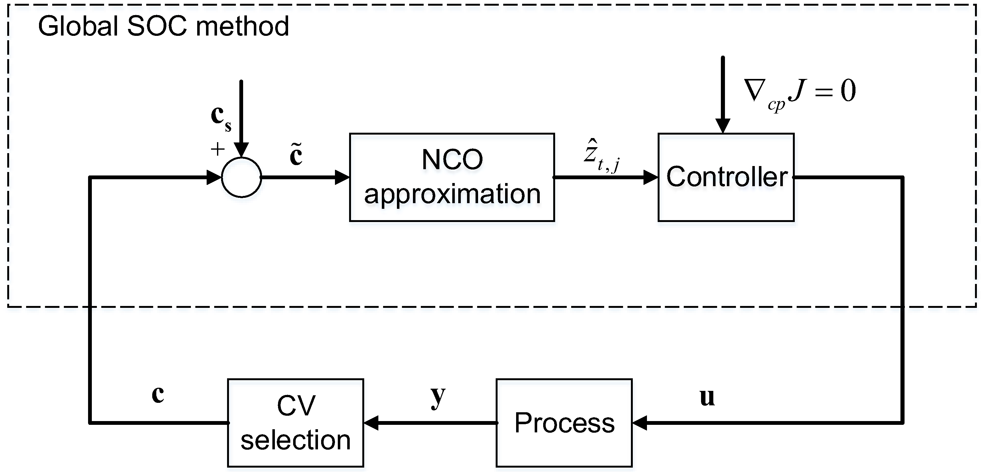
The block diagram of the global SOC method is shown in Figure 2.
In this section, a global SOC method was proposed for the selection of CVs that is based on the approximation of necessary conditions of optimality (NCO) over the entire operating region. The selected CVs are globally valid compared to the local SOC method. Additionally, the proposed method does not require the second order derivative information, therefore it is numerically more reliable and robust. In the next section, a retrofit hierarchical architecture (HA) combining the fast ESC and global SOC is proposed and elaborated.
4. A Retrofit HA Integrating RTO and Control
Considering the differences between ESC and SOC, in general, the former is a model-free scheme that requires the cost measurements to estimate the gradient information based on the local linear least-squares method. In contrast, SOC is a CVs selection scheme that needs no cost measurement, but rather the process simulation model offline to minimize economic loss compared to optimal operation. Furthermore, the SOC scheme can quickly reject the expected disturbances since it works in a feedback fashion, whereas the ESC scheme can handle plant-model mismatch or other unexpected disturbances.
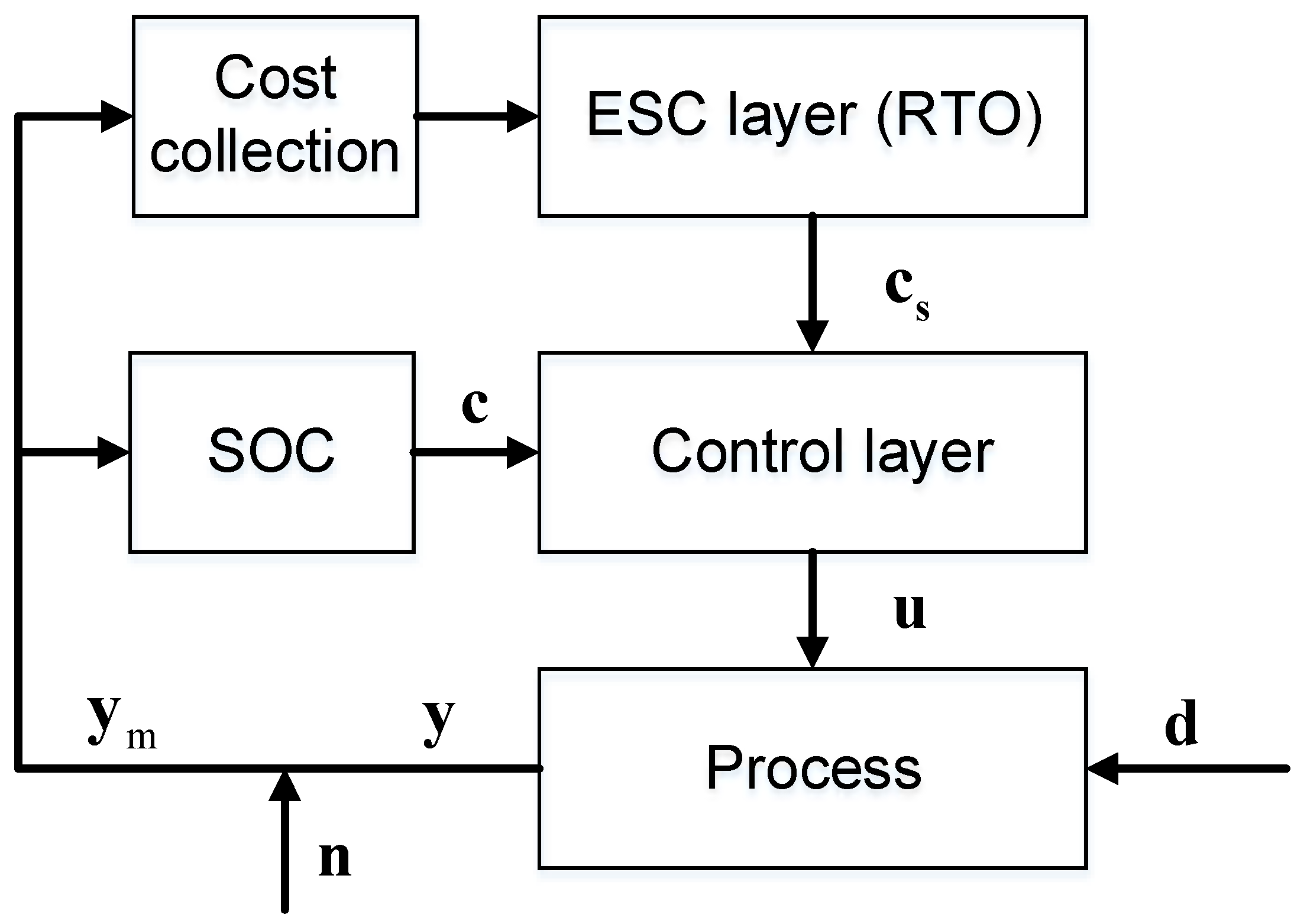
To include both merits from the ESC and SOC schemes, a retrofit HA for RTO and control integration is proposed in this section. Since the time scale in the RTO layer and control layer is different, the ESC scheme fits better in the slower RTO layer to improve the economic performance, while the SOC scheme fits better to integrate the RTO and control layers at a higher frequency. The proposed HA is shown in Figure 3.
The proposed HA contains the following features:
- (1)
- An ESC scheme is employed in the upper layer as an alternative to online model-based real-time optimization techniques. The computational burden is reduced since it is a data-driven approach based on the local linear least-squares method. In addition, incorporating the plant dynamics during the gradient estimation removes the time scale separation between the plant dynamics and the excitation signal, which leads to a faster convergence compared to the classical ESC approach. More importantly, the ESC layer can handle the plant-model mismatch and reduce the steady-state loss by adjusting the set-points.
- (2)
- A SOC scheme is configured with the lower control layer, which can significantly benefit the ESC layer. It should be noted that there are some inherent shortcomings in the ESC scheme. Any a priori information about the process is ignored and the convergence rate is slow in the presence of expected disturbances. The proposed hierarchical architecture combining the ESC and SOC circumvent the above shortcomings of ESC. More precisely, when the expected disturbances occur, the SOC scheme can make a fast adjustment such that the loss is under an acceptable level, whereas in the case where the plant-model mismatch or other unexpected disturbances enter into the process, the action is mainly attributed to the upper ESC layer and the true optimum will be achieved.
- (3)
- Convergence (stability) analysis is another important issue. In this part, we discuss the convergence issue. As mentioned in Section 2, although the fast ESC scheme effectively eliminates the time scale separation between the plant dynamics and the excitation signal, the integral adaptation gain of the ESC scheme must be selected as small to ensure a clear time scale separation between the dither and convergence to the optimum. To this end, there are two time scales in the ESC layer, namely, fast (plant dynamics and dither) and slow (convergence to the optimum). In the proposed retrofit HA, the SOC scheme configured with the lower control layer belongs to the fast time scale [9]. The convergence (stability) results from the least-squares based ESC [10] require a smooth control action parameterized by a performance parameter, which is used by the ESC controller. In the proposed HA, the smooth control action is given by the SOC scheme and the performance parameter is the set-points passed from the ESC layer. In conclusion, the existing convergence results from reference [10] can be applied to the proposed HA under two conditions: (a) the control layer configured with SOC is closed-loop stable; (b) the product of integral adaptation gain and the length of the moving window must be small enough. It is intuitive that a small value of the product guarantees the measurements used for gradient estimation is in the small neighborhood of the current operating point. The gradient estimation error can be bounded if the selected moving window length N is sufficiently small, which allows the chosen integral gain to be large (since only the product should be small), leading to arbitrary, fast convergence. However, in the general case, the adaptation gain should be chosen small such that the performance remains close to the steady state when seen from the upper ESC layer. The detailed convergence (stability) proof which relies on the Lyapunov–Razumikhin theorem can be found in reference [10].
In summary, the SOC scheme not only stabilizes the process, but also drives the process to a near optimal region with an acceptable steady-state loss, whereas when the loss becomes unacceptable or plant-model mismatch occurs, the ESC layer will take actions by adjusting the set-points to reduce them. The major properties show that the model-free ESC and the model-based SOC concepts are complementary rather than competitive.
The procedures for the implementation of a retrofit HA are summarized as follows:
- Collect the last N transient measurements of cost data and input data (also known as the set-points to the lower control layer).
- Estimate the steady-state gradient around the current operating point based on Equations (5) and (7).
- Keep the steady-state gradient at the zero value under an integral control action and update the set-points to the lower control layer.
- Determine and sample the entire operating space using independently generated inputs, disturbances and random noises.
- Calculate the compressed NCO, zj and matrix Y from a process simulation model offline.
- Fit the CVs and calculate the regression parameters by linear least-squares Formula (21).
- Keep the selected CVs at the zero value under a simple feedback control law and update the MVs to the lower plant layer as the process input.
5. Case Study
5.1. Process Description
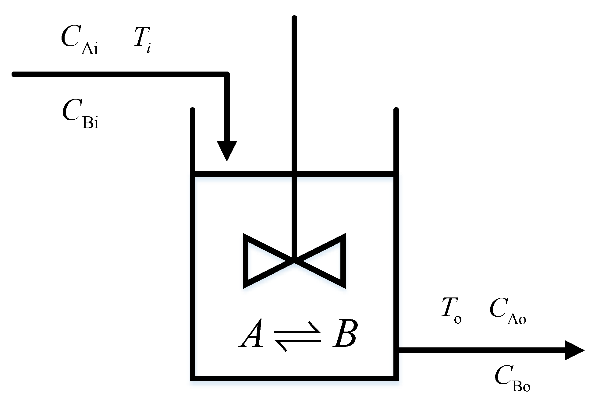
The continuous stirred tank reactor (CSTR) with a reversible exothermic reaction has been extensively investigated [30,33]. A schematic diagram of the CSTR is shown in Figure 4.
According to the law of conservation of mass and energy, the following ordinary differential equations can be obtained to model the dynamic behavior of the system [30]:
where denote the inlet A concentration, inlet B concentration and inlet stream temperature, respectively, and denote the outlet A concentration, outlet B concentration and outlet stream temperature, respectively, is the residence time. r represents the reaction rate, which is defined as
The manipulated variables u, disturbance variables d and measurement variables y of the exothermic reaction process are
The measurement noise is ±0.01 (mol∙L−1) for concentrations and , and ±0.1 K for temperatures and . The state-input constraints are
The objective is to minimize the cost function , which is defined as
where the first term of represents the cost of heating the input stream and the second term is the negative profit of the desired product B.
The nominal values for the exothermic reaction process are listed in Table 1.
To illustrate the effectiveness of the proposed method, first, we applied the fast ESC scheme alone to control the exothermic reaction process and compared it with the classical ESC scheme [9], with a special focus on the convergence time to the optimum. Then, we adopted the global SOC scheme alone to control the process and compared it with the local SOC scheme [20], with a special focus on the average loss over the entire operating space. Finally, we used a retrofit HA combining the fast ESC and global SOC to control the process and compared it with the ESC scheme alone, the SOC scheme alone, simultaneously under the same disturbance conditions, which demonstrates the superiority of the proposed methodology.
5.2. Fast ESC Scheme
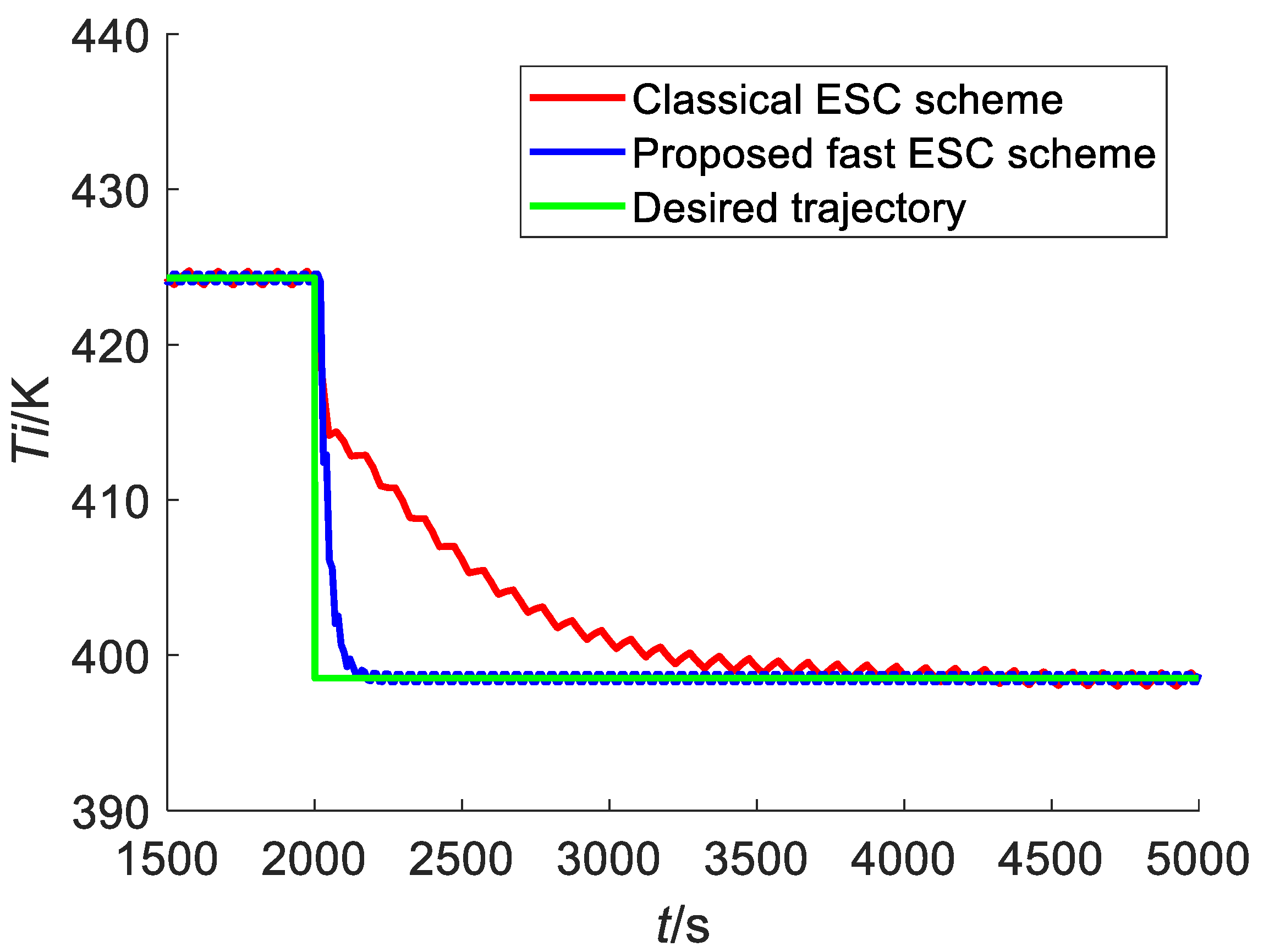
In this subsection, the fast ESC scheme proposed in Section 2 is compared with a classical ESC scheme [9] to control the exothermic reaction process. An additional sinusoidal signal with an amplitude of 0.5 K and a time period of 40 s is added to the classical ESC scheme, and an additional pseudo-random binary sequence signal with an amplitude of 0.5 K is added to the fast ESC scheme, the measurements are assumed to be available with the sample time of 10 s, the adaptation gains of are 0.3 and 2 for the classical ESC and the proposed fast ESC, respectively. The total simulation time is 5000 s with disturbances from 1 (mol∙L−1) to 0.6 (mol∙L−1) and from 0 (mol∙L−1) to 0.4 (mol∙L−1) at time t = 2000 s. The comparison of the input variables using both schemes is shown in Figure 5.
It can be clearly seen that both ESC schemes converge to the same steady-state input value, which is 398.53 K, however, the classical ESC scheme has a significantly slower convergence compared to the proposed fast ESC scheme due to the steady-state wait time. The proposed ESC scheme converges to the optimum within 200 s, whereas the classical ESC scheme takes more than 2000 s to converge. This example clearly shows the effectiveness of the proposed fast ESC over classical ESC.
5.3. Global SOC Scheme
In this subsection, the global SOC scheme proposed in Section 3.2 is compared with a local SOC scheme [20]. In this case, there is only one degree of freedom, such that only one CV needs to be selected. All four measurements are included in the CV function. In the local SOC scheme, the process model is used offline to calculate the optimal sensitive matrix .
The matrices and are evaluated at the nominal point, which is shown as
The diagonal matrices with the expected magnitudes of the disturbance and the measurement noise , which yields,
The analytical solution of the selection matrix for the local SOC scheme is with the average loss . We also investigated the condition without measurement noises, the result is with the average loss .
In the global SOC scheme, the input variables are divided equally into 10 parts and the total sample number is . From the offline calculation, the matrix in Equation (19) can be obtained, but the result is not given due to the space limitation. The selection matrix for the global SOC scheme can be calculated by Formula (21), which is with the average loss . Similarly, the result without measurement noise is with the average loss . For a clear comparison, the average loss, maximum loss and standard deviation for the above four scenarios are listed in Table 2.
From the above results, we can clearly see that compared to the local SOC scheme, the average loss, maximum loss and standard deviation for the global SOC scheme has been significantly reduced, e.g., the average losses are reduced by 87.6% with measurement noise and 86.3% without measurement noise, respectively. It should also be noted that the losses and standard deviations with measurement noise are larger than that without noise. This example clearly shows the superiority of the proposed global SOC over the local SOC in the sense that the selected CVs are globally valid.
5.4. A Retrofit HA Combining the Fast ESC and Global SOC
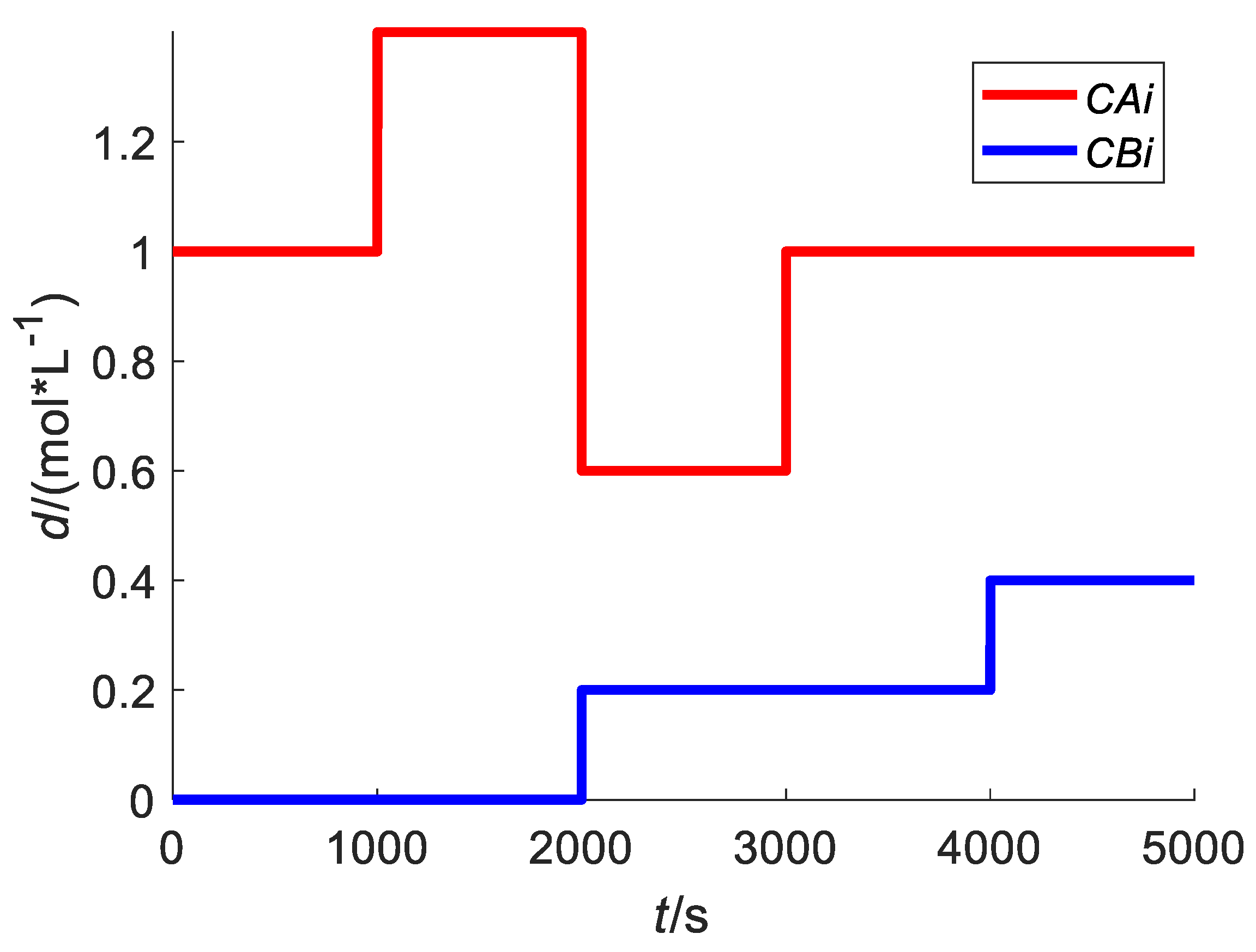
In this subsection, a retrofit HA combining the fast ESC and global SOC is considered. An additional pseudo-random binary sequence signal with an amplitude of 0.5 K is added to the input signal, the measurements are assumed to be available with a sample time of 25 s, the adaptation gains are 0.12 and 3 for the fast ESC scheme and the global SOC scheme, respectively. The expected disturbance scenarios are designed as after 1000 s at the nominal value with a step change of 0.4 (mol∙L−1) that occurs in the inlet A concentration. At t = 2000 s, a step change of −0.8 (mol∙L−1) occurs in the inlet A concentration and a step change of 0.2 (mol∙L−1) occurs in the inlet B concentration. At t = 3000 s, a step change of 0.4 (mol∙L−1) occurs in the inlet A concentration. At t = 4000 s, a step change of 0.2 (mol∙L−1) occurs in the inlet B concentration as shown in Figure 6.
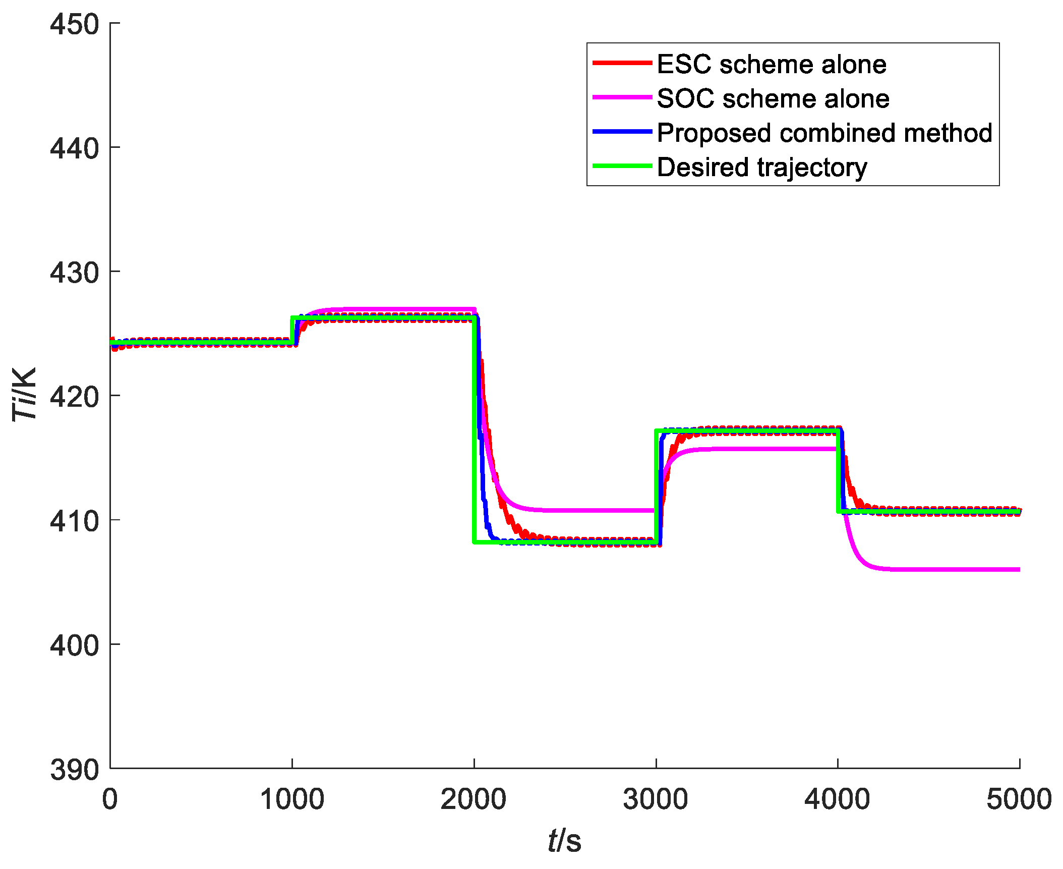
A comparison of the input variables using the fast ESC scheme alone (at the same conditions as in Section 5.2), the global scheme alone (at the same conditions as in Section 5.3) and the proposed combined method is shown in Figure 7.
It can be clearly seen that both the ESC scheme and combined method converge to the same steady-state value, which is 424.29 k for 0~1000 s, 426.27 k for 1000~2000 s, 408.2 k for 2000~3000 k, 417.17 k for 3000~4000 k and 410.67 k for 4000~5000 k, respectively. However, steady-state losses differ between the SOC scheme and the other two schemes. The steady-state losses for the SOC scheme are 0.11 k for 0~1000 s, 0.68 k for 1000~2000 s, 2.54 k for 2000~3000 k, 1.47 k for 3000~4000 k and 4.68 k for 4000~5000 k. It was also clearly shown that for 2000–3000 s and 3000–4000 s, the convergence rate of the combined method is faster than the other two schemes.
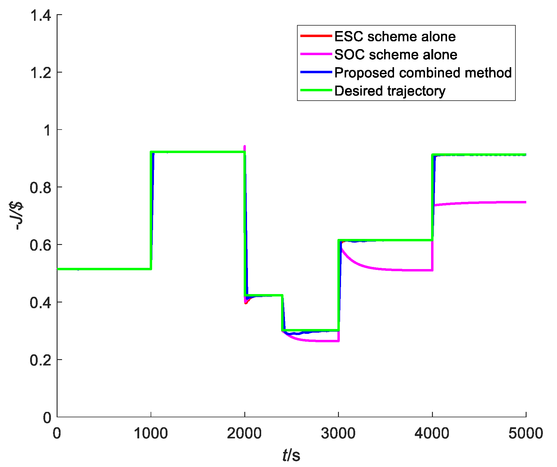
In addition, it is also necessary to compare the profits among the three methods in the presence of plant-model mismatch (structural uncertainty). Considering the plant-model mismatch, more specifically, a step change of 3% in the activation energy E1 (structural mismatch) occurs at time 2400 s, a comparison of the profits (negative cost ) of these methods is shown in Figure 8.
It was shown that the plant-model mismatch reduces the desired profit value from 0.4237 to 0.3022 at time 2400 s. The reason is that the structural uncertainty reduces the reaction rate for the exothermic process. Nonetheless, the combined method and the ESC scheme alone performed similarly in terms of the profit and both outperform the SOC scheme alone, which was anticipated since they both inherit the good features of the model-free approach, and more importantly, as we see from Figure 7, the combined method provides moderate and smoother input usage than the ESC scheme alone. The above results demonstrate the superiority of the proposed methodology.
6. Conclusions
The main contribution of this work is a retrofit HA for real-time optimization and control integration, which demonstrates that ESC and SOC are complementary rather than competitive. The features of the proposed HA can be summarized as follows. (1) A fast ESC scheme using transient measurements that is employed in the upper RTO layer, which can effectively suppress the impact of plant-model mismatch and steady-state wait time. The time scale separation between the plant dynamics and the excitation signal was removed by using transient measurements during the gradient estimation. (2) A global SOC scheme is configured with the control layer to select the appropriate CVs, which provide a moderate reaction to expected disturbances and maintain the process in a near optimal region. The selected CVs are globally valid compared to the local SOC method since it is based on the approximation of NCO over the entire operating space. (3) A linear least-squares regression technique is adopted in both the ESC and SOC schemes, which does not require the second order derivative information, therefore it is numerically more reliable and robust.
An exothermic reaction process was investigated to illustrate the effectiveness of the proposed methodology. The results show that the proposed method inherits the advantages of each individual method, i.e., quickly rejecting disturbances whose characteristics are known, and converging to the optimal operating point in the presence of unknown disturbances. Future work may consider more sophisticated and realistic cases such as the issue of the calculation of the ARX model with measurement noise in the process industry, and how to deal with the changes in the active set is also worthy of further investigation.
Author Contributions
Conceptualization, X.L. and X.L; methodology, X.L.; software, X.L.; validation, X.L., L.X. and H.S.; data curation, X.L.; writing—original draft preparation, X.L.; writing—review and editing, X.L., L.X. and X.L.; supervision, L.X. and H.S.; funding acquisition, H.S. All authors have read and agreed to the published version of the manuscript.
Funding
This research was funded by the National Key Research and Development Program of China (grant numbers: 2016YFB0303404), and the National Natural Science Foundation of China (grant numbers: 61533013).
Acknowledgments
The authors gratefully acknowledge the anonymous reviewers for the insightful comments and suggestions, which improved the quality of this paper to a large extent. Additionally, the first, second, and fourth authors gratefully acknowledge financial support from the National Key Research and Development Program of China (grant numbers: 2016YFB0303404), and the National Natural Science Foundation of China (grant numbers: 61533013).
Conflicts of Interest
The authors declare no conflict of interest.
Abbreviations
The following abbreviations are used in this manuscript:
| HA | Hierarchical Architecture |
| RTO | Real-Time Optimization |
| ESC | Extremum-Seeking Control |
| SOC | Self-Optimizing Control |
| NCO | Necessary Conditions of Optimality |
| CVs | Controlled Variables |
| MPC | Model Predictive Controllers |
| PID | Proportional Integral-Derivative |
| SRTO | Steady-state Real-Time Optimization |
| DRTO | Dynamic Real-Time Optimization |
| EMPC | Economic Model Predictive Control |
| MA | Modifier Adaptation |
| ARX | Auto Regression Exogenous |
| MVs | Manipulate Variables |
| KKT | Karush−Kuhn−Tucker |
| CSTR | Continuous Stirred Tank Reactor |
References
- Mercangoz, M.; Doyle, F.J., III. Real-time optimization of the pulp mill benchmark problem. Comput. Chem. Eng. 2008, 32, 789–804. [Google Scholar] [CrossRef]
- Engell, S. Feedback control for optimal process operation. J. Process Control 2007, 17, 203–219. [Google Scholar] [CrossRef]
- Skogestad, S. Control structure design for complete chemical plants. Comput. Chem. Eng. 2004, 28, 219–234. [Google Scholar] [CrossRef]
- Skogestad, S. Plantwide control: The search for the self-optimizing control structure. J. Process Control 2000, 10, 487–507. [Google Scholar] [CrossRef]
- François, G.; Srinivasan, B.; Bonvin, D. Use of measurements for enforcing the necessary conditions of optimality in the presence of constraints and uncertainty. J. Process Control 2005, 15, 701–712. [Google Scholar] [CrossRef] [Green Version]
- Kumar, V.; Kaistha, N. Hill-climbing for plantwide control to economic optimum. Ind. Eng. Chem. Res. 2014, 53, 16465–16475. [Google Scholar] [CrossRef]
- Chachuat, B.; Srinivasan, B.; Bonvin, D. Adaptation strategies for real-time optimization. Comput. Chem. Eng. 2009, 33, 1557–1567. [Google Scholar] [CrossRef]
- Tan, Y.; Moase, W.H.; Manzie, C. Extremum seeking from 1922 to 2010. In Proceedings of the 29th Chinese Control Conference (CCC), Beijing, China, 29–31 July 2010; IEEE: New York, NY, USA, 2010; pp. 14–26. [Google Scholar]
- Krstic, M.; Wang, H.H. Stability of extremum seeking feedback for general nonlinear dynamic systems. Automatica 2000, 36, 595–601. [Google Scholar] [CrossRef]
- Hunnekens, B.G.B.; Haring, M.A.M.; van de Wouw, N. A dither-free extremum-seeking control approach using 1st-order least-squares fits for gradient estimation. In Proceedings of the 53rd IEEE Conference on Decision and Control, Los Angeles, CA, USA, 15–17 December 2014; IEEE: New York, NY, USA, 2014; pp. 2679–2684. [Google Scholar]
- Chioua, M.; Srinivasan, B.; Guay, M. Performance improvement of extremum seeking control using recursive least square estimation with forgetting factor. IFAC PapersOnLine 2016, 49, 424–429. [Google Scholar] [CrossRef]
- Choi, J.Y.; Krstic, M.; Ariyur, K.B. Extremum seeking control for discrete-time systems. IEEE Trans. Autom. Control 2002, 47, 318–323. [Google Scholar] [CrossRef]
- Fu, L.; Özgüner, Ü. Extremum seeking with sliding mode gradient estimation and asymptotic regulation for a class of nonlinear systems. Automatica 2011, 47, 2595–2603. [Google Scholar] [CrossRef]
- Ghaffari, A.; Krstić, M.; NešIć, D. Multivariable Newton-based extremum seeking. Automatica 2012, 48, 1759–1767. [Google Scholar] [CrossRef]
- Krishnamoorthy, D.; Foss, B.; Skogestad, S. Real-Time Optimization under Uncertainty Applied to a Gas Lifted Well Network. Processes 2016, 4, 52. [Google Scholar] [CrossRef] [Green Version]
- Darby, M.L.; Nikolaou, M.; Jones, J. RTO: An overview and assessment of current practice. J. Process Control 2011, 21, 874–884. [Google Scholar] [CrossRef]
- Ellis, M.; Durand, H.; Christofides, P.D. A tutorial review of economic model predictive control methods. J. Process Control 2014, 24, 1156–1178. [Google Scholar] [CrossRef]
- Camara, M.; Soares, R.; Feital, T. Numerical aspects of data reconciliation in industrial applications. Processes 2017, 5, 56. [Google Scholar] [CrossRef] [Green Version]
- Larsson, T.; Hestetun, K.; Hovland, E. Self-optimizing control of a large-scale plant: The Tennessee Eastman process. Ind. Eng. Chem. Res. 2001, 40, 4889–4901. [Google Scholar] [CrossRef]
- Halvorsen, I.J.; Skogestad, S.; Morud, J.C. Optimal selection of controlled variables. Ind. Eng. Chem. Res. 2003, 42, 3273–3284. [Google Scholar] [CrossRef]
- Alstad, V.; Skogestad, S. Null space method for selecting optimal measurement combinations as controlled variables. Ind. Eng. Chem. Res. 2007, 46, 846–853. [Google Scholar] [CrossRef]
- Alstad, V.; Skogestad, S.; Hori, E.S. Optimal measurement combinations as controlled variables. J. Process Control 2009, 19, 138–148. [Google Scholar] [CrossRef]
- Kariwala, V. Optimal measurement combination for local self-optimizing control. Ind. Eng. Chem. Res. 2007, 46, 3629–3634. [Google Scholar] [CrossRef]
- Kariwala, V.; Cao, Y.; Janardhanan, S. Local self-optimizing control with average loss minimization. Ind. Eng. Chem. Res. 2008, 47, 1150–1158. [Google Scholar] [CrossRef]
- Kariwala, V.; Skogestad, S. Branch and bound methods for control structure design. Comput. Aided Chem. Eng. 2006, 21, 1371. [Google Scholar]
- Cao, Y.; Kariwala, V. Bidirectional branch and bound for controlled variable selection: Part I. Principles and minimum singular value criterion. Comput. Chem. Eng. 2008, 32, 2306–2319. [Google Scholar] [CrossRef] [Green Version]
- Kariwala, V.; Cao, Y. Bidirectional branch and bound for controlled variable selection. Part II: Exact local method for self-optimizing control. Comput. Chem. Eng. 2009, 33, 1402–1412. [Google Scholar] [CrossRef] [Green Version]
- Kariwala, V.; Cao, Y. Bidirectional branch and bound for controlled variable selection Part III: Local average loss minimization. IEEE Trans. Ind. Inf. 2010, 6, 54–61. [Google Scholar] [CrossRef] [Green Version]
- Yelchuru, R.; Skogestad, S. Convex formulations for optimal selection of controlled variables and measurements using mixed integer quadratic programming. J. Process Control 2012, 22, 995–1007. [Google Scholar] [CrossRef]
- Ye, L.; Cao, Y.; Li, Y. Approximating necessary conditions of optimality as controlled variables. Ind. Eng. Chem. Res. 2012, 52, 798–808. [Google Scholar] [CrossRef]
- Ye, L.; Cao, Y.; Yuan, X. Global approximation of self-optimizing controlled variables with average loss minimization. Ind. Eng. Chem. Res. 2015, 54, 12040–12053. [Google Scholar] [CrossRef]
- Jaschke, J.; Cao, Y.; Kariwala, V. Self-optimizing control–A survey. Annu. Rev. Control 2017, 43, 199–223. [Google Scholar] [CrossRef] [Green Version]
- Jaschke, J.; Skogestad, S. NCO tracking and self-optimizing control in the context of real-time optimization. J. Process Control 2011, 21, 1407–1416. [Google Scholar] [CrossRef]
- Ye, L.; Cao, Y.; Ma, X. A novel hierarchical control structure with controlled variable adaptation. Ind. Eng. Chem. Res. 2014, 53, 14695–14711. [Google Scholar] [CrossRef]
- Ye, L.; Miao, A.; Zhang, H. Real-time optimization of gold cyanidation leaching process in a two-layer control architecture integrating self-optimizing control and modifier adaptation. Ind. Eng. Chem. Res. 2017, 56, 4002–4016. [Google Scholar] [CrossRef]
- Lersbamrungsuk, V.; Srinophakun, T.; Narasimhan, S. Control structure design for optimal operation of heat exchanger networks. AIChE J. 2008, 54, 150–162. [Google Scholar] [CrossRef]
- Hu, W.; Umar, L.M.; Kariwala, V.; Xiao, G. Local self-optimizing control with input and output constraints. In Proceedings of the 18th World Congress of the International Federation of Automatic Control (IFAC), Milano, Italy, 28 August–2 September 2011; IEEE: Helsinki, Finland, 2011; pp. 9850–9855. [Google Scholar]
Figure 1.
A block diagram of the fast extremum-seeking control (ESC) approach.

Figure 2.
A block diagram of the global self-optimizing control (SOC) method.

Figure 3.
The proposed hierarchical architecture.

Figure 4.
A schematic diagram of the continuous stirred tank reactor.

Figure 5.
A comparison of the input variables using classical ESC and the proposed fast ESC.

Figure 6.
Disturbance scenarios.

Figure 7.
A comparison of the input variables using the ESC scheme alone, the SOC scheme alone and the proposed combined method.
Figure 7.
A comparison of the input variables using the ESC scheme alone, the SOC scheme alone and the proposed combined method.

Figure 8.
A comparison of the profits using the ESC scheme alone, the SOC scheme alone, and the proposed combined method.
Figure 8.
A comparison of the profits using the ESC scheme alone, the SOC scheme alone, and the proposed combined method.


Table 1.
Nominal values for the exothermic reaction process.
| Variable | Nominal Value | Unit |
|---|---|---|
| CAo | 0.498 | mol∙L−1 |
| CBo | 0.502 | mol∙L−1 |
| To | 426.803 | K |
| CAi | 1 | mol∙L−1 |
| CBi | 0 | mol∙L−1 |
| Ti | 424.292 | K |
| F | 1 | mol∙min−1 |
| τ | 60 | s |
Table 2.
Economic loss comparison.
| Scenarios | Average Loss | Maximum Loss | Standard Deviation |
|---|---|---|---|
| local SOC with noise | 10.0355 | 90.6237 | 14.7173 |
| local SOC without noise | 8.6377 | 65.3685 | 12.6398 |
| global SOC with noise | 1.2439 | 8.5157 | 1.3853 |
| global SOC without noise | 1.1834 | 6.2701 | 1.2041 |
© 2020 by the authors. Licensee MDPI, Basel, Switzerland. This article is an open access article distributed under the terms and conditions of the Creative Commons Attribution (CC BY) license (http://creativecommons.org/licenses/by/4.0/).
Share and Cite
MDPI and ACS Style
Li, X.; Xie, L.; Li, X.; Su, H. A Retrofit Hierarchical Architecture for Real-Time Optimization and Control Integration. Processes 2020, 8, 181. https://0-doi-org.brum.beds.ac.uk/10.3390/pr8020181
AMA Style
Li X, Xie L, Li X, Su H. A Retrofit Hierarchical Architecture for Real-Time Optimization and Control Integration. Processes. 2020; 8(2):181. https://0-doi-org.brum.beds.ac.uk/10.3390/pr8020181
Chicago/Turabian StyleLi, Xiaochen, Lei Xie, Xiang Li, and Hongye Su. 2020. "A Retrofit Hierarchical Architecture for Real-Time Optimization and Control Integration" Processes 8, no. 2: 181. https://0-doi-org.brum.beds.ac.uk/10.3390/pr8020181
Note that from the first issue of 2016, this journal uses article numbers instead of page numbers. See further details here.