Gray-box Soft Sensors in Process Industry: Current Practice, and Future Prospects in Era of Big Data


1
Department of Chemical and Materials Engineering, National University of Sciences and Technology, Islamabad 44000, Pakistan
2
US Pakistan Center for Advanced Studies in Energy, National University of Sciences and Technology, Islamabad 44000, Pakistan
3
Department of Systems Science, Kyoto University, Kyoto 606-8501, Japan
4
Department of Chemical, Polymer and Composite Materials Engineering, University of Engineering and Technology, Lahore (New Campus) 39021, Pakistan
*
Author to whom correspondence should be addressed.
Processes 2020, 8(2), 243; https://0-doi-org.brum.beds.ac.uk/10.3390/pr8020243
Submission received: 18 December 2019
/
Revised: 21 January 2020
/
Accepted: 10 February 2020
/
Published: 20 February 2020
(This article belongs to the Special Issue Advanced Methods in Process and Systems Engineering)
Abstract
:Virtual sensors, or soft sensors, have greatly contributed to the evolution of the sensing systems in industry. The soft sensors are process models having three fundamental categories, namely white-box (WB), black-box (BB) and gray-box (GB) models. WB models are based on process knowledge while the BB models are developed using data collected from the process. The GB models integrate the WB and BB models for addressing the concerns, i.e., accuracy and intuitiveness, of industrial operators. In this work, various design aspects of the GB models are discussed followed by their application in the process industry. In addition, the changes in the data-driven part of the GB models in the context of enormous amount of process data collected in Industry 4.0 are elaborated.
1. Introduction
Industrial evolution in terms of automation and control has been classified into four major eras, i.e., Industry 1.0, 2.0, 3.0 and 4.0. The introduction of mechanical production facilities led to the first industrial revolution termed as Industry 1.0 which span through an era from the second half of the eighteenth century till the last quarter of the nineteenth century. The second industrial revolution, termed Industry 2.0, started in the 1870s on the emergence of electricity applications and proper management of labor. The digitization introduced around the 1970s helped use advanced electronics and information technology for process automation, which formed the era of Industry 3.0. The current (r)evolution, termed Industry 4.0, is driven by the emergence of concepts, such as cloud-computing, smart sensors, internet of things (IoT), big data analytics, augmented reality, and human–machine interfaces [1,2,3,4,5,6,7,8].
Process sensors also evolved from purely mechanical indicators used in the era of Industry 1.0 to smart sensors of Industry 4.0. In this context, Sensors 4.0 has been coined colloquially to Industry 4.0 [9]. Smart sensors are sensing devices that are equipped with digital features for data processing, storage and efficient transformation of data [10,11,12]. Smart sensors automatized the zero correction, calibration, and scaling of the measured signals by using microprocessors, in contrast to meticulous design, testing, and debugging faced by the conventional analog sensors [13,14,15,16]. The sensing platform of a smartphone is the best example of smart sensing environment; it integrates multiple sensors and makes use of multi-sensory signals based on gyroscopes, accelerators, pressure, and magnetometers sensors. These sensors simultaneously do weather monitoring, step counting, screen orientation, gaming, etc.
The use of smart sensors in the process industry has been demonstrated in several studies [17,18,19,20,21], where internet of things (IoT) devices are used to collect enormous amount of data from process equipment such hydraulic pumps, reactors, heat exchangers, etc. Considering the massive amount of data, data processing is performed before it is passed on for analysis and decision making regarding the process operations.
The data processing methods have to handle the big volume, high frequency, variety and veracity of the data coming from the IoT devices [22,23]. The preprocessing techniques include data wrangling, visualization, sparsity and regularization, optimization, reducing dimensionality, measuring distance, representation learning, and sequential learning [24,25,26,27].
The data collected through the hardware sensors, i.e., thermo-couples, manometers, etc., have been used for monitoring and control of the process. However, three decades ago, the idea of using the data for the development of predictive models emerged [28]. These predictive models were termed soft sensors. The term soft sensor is a combination of two words; “software”, which refers to the fact that the models are usually computer programs, and “sensors” because they serve the same purpose as that of the hardware sensors. Soft sensors are capable of estimating process states that are difficult to measure through hardware sensors due to large measurement delays, technological limitations or high investment costs. Even if hardware sensors can be used, operators have found soft sensors superior to hardware sensors; the soft sensors stabilize operation, reduce energy and materials consumption, and cross-check the performance of an online hardware sensor [29]. Soft sensors can also be used in parallel with the hardware sensor to give additional information [30,31]. The soft sensors are classified into three major categories based on their underlying models namely white-box (WB), black-box (BB) and gray-box (GB) models. WB models are based on process knowledge while the BB models are developed using data collected from the process. The WB models are descriptive and easy for industry operators to interpret. However, they have certain limitations, sometimes they are unable to grasp the true dynamics of a complex industrial process and their prediction accuracy is accompanied by a substantial amount of errors. The BB models, on the other hand, are more accurate in prediction than the WB models, however, they are less intuitive in nature. The GB models integrate the WB and BB models for addressing the concerns, i.e., accuracy and intuitiveness, of industrial operators.
Applications of GB models are found in a variety of domains in process industries such as design, estimation, control, and monitoring. They are applied across the process industries such as iron and steel making [32,33,34,35,36], food processing [37,38,39], oil and gas processing [40,41,42,43,44], chemical, biochemical, and pharmaceutical [45,46,47,48,49,50,51,52,53,54], power plants [55,56,57], water treatment [58,59,60], material processing and energy materials [61,62,63,64] and industrial robots [65,66,67].
The aim of the current study is to do a comprehensive review of the fundamentals of GB soft sensors, their applications in the process industry and prospects in the era of big data analytics; to the best of the authors’ knowledge, no extensive review that addresses all such dimensions is reported in the literature. GB soft sensors application in selected process industries were investigated. The industries were ranked in terms of using GB soft sensors in their process. The pattern in the objectives of the application, the trends in the type of GB model as well as the type of BB methods were analyzed. Finally, the prospects and challenges of GB soft sensors in the era of big data are elaborated.
Section 2 describes fundamentals of soft sensors. The design types of GB models and methodology adopted in this paper are discussed in Section 3 and Section 4, respectively. Applications of GB models in the process industry and their prospects in the era of industry 4.0 are discussed in Section 5 followed by conclusions in Section 6.
2. Fundamentals of Soft Sensors
The fundamentals of three types of soft sensors based on their underlying model, i.e., WB, BB, and GB, are briefly discussed in this section.
The WB models are also referred to as the first principle, “mechanistic”, “analytical”, “phenomenological”, “physical”, “fundamental”, and “parametric” models that describe the underlying laws of science and engineering which govern the process(es) [68]. The WB models rely on natural characteristics, i.e., reaction kinetics, thermodynamics, and fluid properties, and conservation laws, such as mass, energy, and momentum of the target process [69]. The WB models transform the process of knowledge into mathematical formulations [70]. The WB model equations get a form of ordinary or partial differential-algebraic equations with properly defined initial and boundary conditions. Analytical methods or numerical methods are applied to solve the equations keeping in view the complexity of the problem. Some parameters of the WB models can be based on real data to a minor extent [71,72]. For example, Fick’s law, Fourier’s law, Darcy’s law, and ideal gas law are categorized into WB models, but they were initially derived through empirical correlations, based on experimental data. The attempts to efficiently develop process models through simulator, a WB modeling environment, started back in the 1950s. However, the emergence of Process Systems Engineering later in the 1980s intensified the integration of process simulations in the loop of computer-aided design, process control, and optimization [73,74]. The WB models face some challenges such as non-linearity [75,76], uncertainties [77,78], multi-scale (time and physical dimensions) [79], high dimensionality [80], and time delay [81].
The BB models are used to describe complex processes that are difficult for the WB model to handle [82]. Other names used for BB models are “data-based”, “non-parametric”, and “empirical” models [68]. The BB term refers to black-box behaviors of merely mapping the I/O data and its mathematical structure is not necessarily based on natural characteristics of the process [83]. The lack of physical meaning of the BB model structures is considered its disadvantage but this feature also makes the researchers able to model a process in spite of their unawareness of underlying process dynamics [83,84]. With increasing complexities of modeling tasks, emergence of high-speed computing and demand of less complicated and efficient process sensing, a paradigm shift from WB to BB methods, such as artificial neural network (ANN), partial least squares (PLS), support vector machine (SVM), principle component analysis (PCA), and random forests (RF) have been applied [28,82,85]. However, the BB models are expensive in terms of the computational load and time than the WB models. Besides, realizing optimal structure design, accurate parametric values, and lesser intuitiveness have been the major challenges they face [86].
The GB models which emerged in the field of control and system theory in the 1990s combine the WB and the BB techniques [87,88,89]. The GB models are also named “semi-analytical”, “semi-physical”, “semi-parametric”, and “hybrid” models [68]. The hybrid term also represents the integration of two BB models. Thus, all GB models can be referred to as hybrid models, but all hybrid models may not be GB models. The GB models have been used in modeling a variety of processes since its inception [90,91]. GB modeling strategy compensates for the deficiencies of the standalone WB and BB models by adding both accuracy, reliability, and intuitiveness [90].
3. Types of GB Models
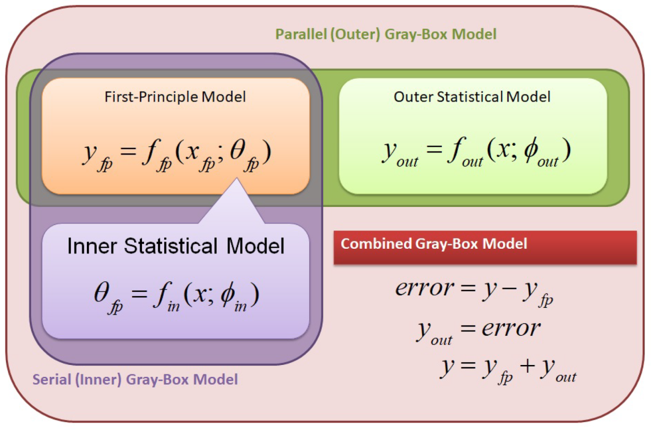
GB models are classified into three categories: parallel, serial and combined gray-box models. A schematic view of GB models’ classification is shown in Figure 1.
The parallel GB model uses BB model to compensate error of a WB model. The BB model in the parallel GB modeling framework is referred as the outer statistical model as it does not affect the internal structure of a WB model. Likewise, the parallel GB approach overcomes the limitations caused by the structure of the first-principle model. The general format of parallel GB mode is represented by the following equation [34]:
where and are vectors of parameters of the WB and BB models, respectively. The is a subset of , and is the prediction of y by using the parallel GB model.
In the parallel GB model, the error of the WB model is compensated, however, parameters of the WB model are kept constant. This simplification sometimes deteriorates the performance of the WB model because some parameters may strongly depend on process conditions. Therefore, the serial GB model is used to update the parameters as functions of process conditions. The serial GB models have higher intuitiveness because the important physical parameters are identified and related to process variables. The serial GB model is represented by the following equation:
where is the vector of the estimated parameters, and is the prediction of y by the serial GB model.
In order to utilize both the internal and external use of the BB models with the WB models, a combined GB model is developed by combing the parallel GB modeling and the serial GB modeling features. In the combined GB model, a prediction error of a serial GB model is compensated by an outer BB model. The combined GB model consists of the WB model, the inner BB model to estimate parameters, and the outer BB model to compensate the prediction error. The combined GB mode is represented by the following equation.
where is a vector of parameters and is the prediction of y through the combined GB model.
4. Methodology
Application of GB soft sensors in iron and steel making, food processing, oil and gas processing, chemical, biochemical, and pharmaceutical, power plants, and sub-processes such as water treatment, material processing, energy materials, and industrial robots were analyzed. In addition, application of GB soft sensors to miscellaneous theoretical case studies of process equipment were investigated. These case studies were lumped into two categories, i.e., reactive systems and heating systems. Google scholar database was used to collect reported studies on GB soft sensors application in the selected process industries in the last fifteen years, i.e., 2005-2019. The industries were ranked in terms of the use of GB soft sensors in their process. The pattern in the objectives, i.e., quality estimation, fault diagnosis, control, etc., of using the GB soft sensors was also investigated. In addition, the type of GB as well as the type of BB methods, i.e., ANN, RF, SVM, etc., were also ranked in terms of their application. Finally, the prospects and challenges of GB soft sensors in the era of big data are elaborated.
5. Current Practice in Process Industry
5.1. Iron and Steelmaking
Sohlberg et al. [32] developed a serial GB model for estimation of exit concentration of hydrochloric acid of the pickling process. Taylor series expansion was used in integration with WB model of the process. In a study by Barrios et al. [33], a parallel GB model was developed for entry temperature estimation of secondary scale breaker (SB). Fuzzy Inference System (FIS) was used for the estimation of the error of the WB model of the process. Okura et al. [92] used a parallel GB model for the estimation of molten steel temperature in a continuous casting process. Partial least squares (PLS) and random forests (RF) were used as BB models. Ahmad et al. [34] developed parallel, serial, and combined GB models to predict and control molten steel temperature in a continuous casting process where RF was used as a BB model. In another study by Ahmad et al. [35], a combined GB model was integrated with a bootstrap filter to predict the probability distribution of molten steel temperature in a continuous casting process under uncertainty. Barrios et al. [36] used ANN-based parallel GB model to estimate scale breaker entry temperature.
5.2. Food Processing
Cubillos et al. [37] developed a serial GB for estimation and control of moisture content in a direct fish-meal rotary dyer where ANN was used as a BB model. Vieira et al. [38] developed a serial GB model for prediction and control of the moisture content of milk powder produced in a spouted bed dryer. ANN was used as BB technique. Saltık et al. [39] used a serial GB for estimation of membrane fouling for an ultrafiltration membrane unit in a whey separation process. Exponential static membrane resistance function was used for the identification of parameters of the WB model of the process.
5.3. Chemical, Biochemical, and Pharmaceutical
Prada-Moraga et al. [45] developed a serial GB for estimation of the growth rate of biomass in a fermentation process. A mixed-integer optimization algorithm Automatic Learning of Algebraic Models (ALAMO) was used to identify the structure and parameters of the model. Wang et al. [46] applied serial GB model of marine alkaline protease fermentation to predict biomass concentration, substrate concentration and relative enzyme activity. Multi-I/O least squares support vector machine (MLSSVM) integrated with an artificial bee colony optimization algorithm was used as a black-box model. Niu et al. [47] applied a parallel GB model for the prediction of substrate concentration, cell concentration, and product concentration of nosiheptide fed-batch fermentation. Least-squares support vector machines were used as a BB model for compensation of error of the WB model of the process. Wu et al. [93] developed a parallel GB method for modeling and control of polymer molecular weight distribution (MWD) of the petrochemical industry. A recurrent neural network (RNN) and an orthogonal polynomial feed-forward neural network (OPFNN) were combined to model the shape of MWD. Johansen et al. [48] investigated the use of a serial GB model to design a control scheme for screw speed of plasticating twin-screw extruder (TSE) of a petrochemical plant. Autoregressive moving average exogenous (ARMAX) structure was used as a BB part of the GB model. Liu et al. [49] proposed a serial GB modeling for prediction and control of melt viscosity of product of a polymer extrusion process of a petrochemical plant. Genetic algorithm was integrated with the WB model to develop the GB model. Everett et al. [50] developed a serial GB model to predict the non-linear behavior of mold cooling. ANN was used to approximate the parameters of state-space model (SSM) of the process. Zahedi et al. [51] used a serial GB model for yield prediction of an extraction process. A neuro-fuzzy technique was used as a black box model for the estimation of Sh number. Cubillos et al. [52] investigated the feasibility of using a serial GB model for Real Time Optimization (RTO) of a Williams-Otto reactor. ANN and GA were integrated with the first-principle model of the reactor to efficiently predict and control the reactor temperature and the flow rate of the component. Pitarc et al. [53] proposed a serial GB model for prediction of overall heat transfer coefficient of heat exchangers in an evaporation plant. Data reconciliation (DR) and polynomial constrained regression approaches were used as BB models. Liu et al. [54] used a serial GB model for estimation of mycelia concentration, sugar concentration and chemical potency of the fermentation process of the pharmaceutical industry where ANN was used as a BB model.
5.4. Power Plants
Zhao et al. [55] developed a serial GB model for estimation of boiler thermal efficiency and NOx concentration of furnace outlet in a coal power plant. Boiler thermal efficiency and NOx concentration of furnace outlet were the outputs of the model. The fast recursive algorithm was used as a BB model. Arahal et al. [56] used a serial GB model to predict and control the temperature of a thermal storage tank of a solar power plant. Simultaneous Perturbation Stochastic Approximation (SPSA) technique was used for parameter identification. Barszcz et al. [57] used a serial GB approach for anomaly detection and control of feed water conditions, i.e., temperature, pressure, flow rate, etc., of a heat exchanger of a coal power plant. ANN was used as a BB model.
5.5. Oil and Gas Processing
Møller et al. [40] investigated the use of a serial GB model for slugging oscillation of a valve control system in the offshore process. Extended Kalman Filter (EKF) was used as a BB model. Onel et al. [41] used a serial GB model for prediction of reactor output composition of steam methane reforming (SMR) microchannel reactor. The non-linear fitting model was used as a BB model. Bram et al. [42] developed a serial GB model to estimate and control the rejected flow rate of a hydro cyclone. The model parameters were estimated through a least-squares method. In a study by Lotfalipour et al. [43], a serial GB model was developed for prediction of CO2 emission in plant-wide facility of oil and gas rig. The least-squares estimation sequence is used as BB technique. Durrani et al. [44] used a serial GB strategy that was devised by integrating ANN with Aspen HYSYS model of crude distillation unit (CDU). ANN was used to estimate parameters, i.e., cut-point temperature, of the CDU model.
5.6. Water Treatment
Stentoft et al. [58] developed a serial GB model for prioritizing aeration in economical schedule in wastewater treatment plants. The genetic algorithm (GA) was integrated with stochastic differential equations, based on the WB model of the process. Stentoft et al. [59] used the serial modeling framework to predict ammonium nitrate concentrations in a small recirculating Water Resource Recovery Facilities (WRRFs). Extended Kalman Filter (EKF) was used for parameters estimation. Dragoi et al. [60] used serial, parallel and combined GB models to predict dissolution rate of solute, i.e., sodium carbonate, urea, and sodium bicarbonate. ANN was used as BB model.
5.7. Material Processing and Energy Materials
Li et al. [61] developed a serial GB model for estimating the possibility of the datum in materials authorization (RMA) process in a TFT-LCD industry. The fuzzy membership function (MF) value was used as a representative of the possibility of the datum. Ordinary least square method was used for parameters estimation. Rad et al. [62] applied a serial GB model for prediction and control of temperature of a thermotronic system. Simulink Design Optimization Tool (SDO) was used for parameter identification. Masoudinejad et al. [63] investigated the use of a serial GB model of a photovoltaic (PV) cell for low illuminance indoor lighting conditions in a material handling and warehousing. Internal parameters were identified using a least squares method. Liu et al. [64] used a serial GB model for estimating the irradiation angle of sensor prototype in solar energy harvesting industrial facility. A simple least-squares method was used to predict the parameters of the WB model.
5.8. Industrial Robot
Wernholt et al. [65] developed a serial GB model for prediction of motor angular speed of an industrial robot. Weighted logarithmic least squares were used as a BB model. Knoblach et al. [94] used a serial GB model for prediction and control of the motor velocity of an industrial robot. Weighted logarithmic least squares (WLLS) was used as a BB model. Ayala et al. [66] used a serial GB for prediction of the deflection of a piezoelectric micromanipulator through ANN with data acquired in a laboratory setup. Wernholt et al. [67] investigated the use of GB model for prediction and control of the machine position of a robot. Weighted nonlinear least squares and weighted logarithmic least squares were used for parameter estimation.
5.9. Miscellaneous
5.9.1. Reactive Systems
In a study by Acuña et al. [95], Least-Square Support Vector Machine (LS-SVM) was used to develop a serial GB model for prediction of the degree of progress of reaction of a Continuous Stirred Tank Reactor (CSTR). In another study by Acuña et al. [96], serial GB model was developed for prediction of the degree of progress of the reaction in CSTR. Least-square support vector machine and genetic algorithms were used for enhancing the performance of the WB model of the CSTR. Porru et al. [97] developed a serial GB model for prediction of product composition of a heterogeneous gas-solid reactor. ANN and extended Kalman filter (EKF) was integrated with the WB model of the reactor. Xiong et al. [98] investigated the use of a parallel GB model for prediction and control of heat release inside a simulated exothermic batch reactor. ANN was used for compensation of error of the WB model of the reactor. Hourfar et al. [99] used a serial GB model that was developed for prediction and control of the temperature of the nonlinear CSTR benchmark process. ANN was used to estimate parameters of the WB model of the CSTR. Zanardo et al. [100] developed a serial GB model for prediction of molar flow rates of NOx and NH3 at the outlet of a Selective Catalytic Reduction (SCR). Auto-regressive with eXogenous Input (ARXIs) was used for parameter identification. Acuña et al. [101] used a MATLAB toolbox for the design, construction and validation of a serial GB models of a CSTR. ANN model was used for the estimation of parameters of the WB model. Barkman [102] developed a serial GB model to estimate concentration distributions in the context of modeling a reaction-advection-diffusion system and was evaluated on a one-dimensional and a two-dimensional instance of the reaction system. ANN was used to estimate the parameter of the reaction model.
5.9.2. Heat Treatment Processes
Pearson et al. [103] devised a serial GB model approach for three classes of block-oriented models: Wiener models, Hammerstein models, and the feedback block-oriented models. The approach was illustrated for prediction and control of heat release inside the reactor distillation column where the least square method was used to estimate parameters of the model. Weyer et al. [104] used a serial GB model for fault diagnosis, i.e., settled material breaking away from the heat transfer surface, of a heat exchanger. The recursive least-squares identification method was used as BB model. Miao et al. [105] developed a serial GB model for the prediction of outlet temperatures of plate heat exchangers. A parameter identification method was established through the Taylor series. Cubillos et al. [106] developed a serial GB model to estimate heat losses and control of the temperature of the combustion chamber of a pilot-scale vibrating fluidized dryer. ANN was used for parameters estimation. Farooq et al. [107] developed a serial GB model to predict the temperature of stratified virtual layers in a boiler. The nonlinear least-squares optimization method and trust-region reflective algorithm were used for the estimation of the WB model’s parameters. Aprile et al. [108] devised a serial GB model for prediction of gas utilization efficiency and the heating capacity of a water-source gas-driven absorption heat pump. Linear interpolation was used for parameter identification. Sossan et al. [109] developed a serial GB model for predictive control (MPC) of electricity consumption of a refrigeration system. Stochastic differential equations (SDEs) estimated by maximum likelihood estimation (MLE) was used as a BB model. Petersen et al. [110] investigated the use of a serial GB modeling for prediction of the residual moisture, the temperature, and the particle size in each stage for complete drying process in a multi-stage spray dryer. The WB model’s parameters were identified using the least-squares method. De-Moor et al. [111] used a serial GB strategy for the prediction of mass concentration and temperature within an imperfectly mixed fluid. The total least square method was used to identify parameters of the WB model.
5.10. Application Summary
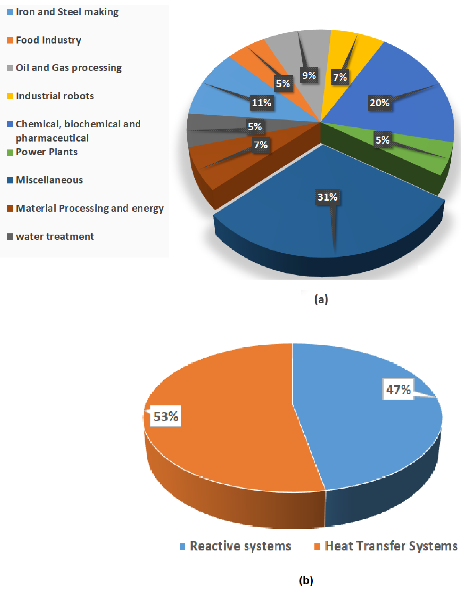
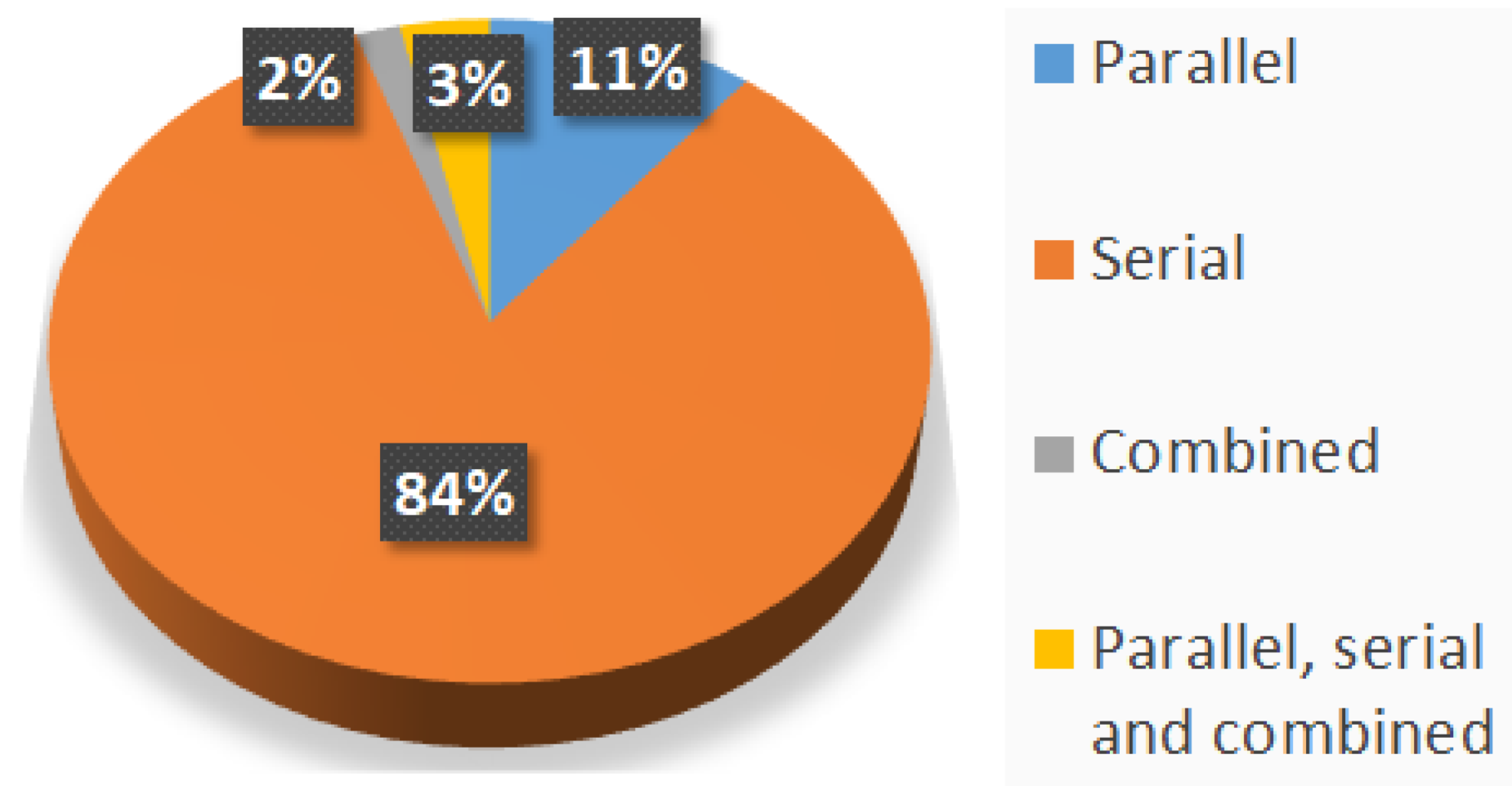
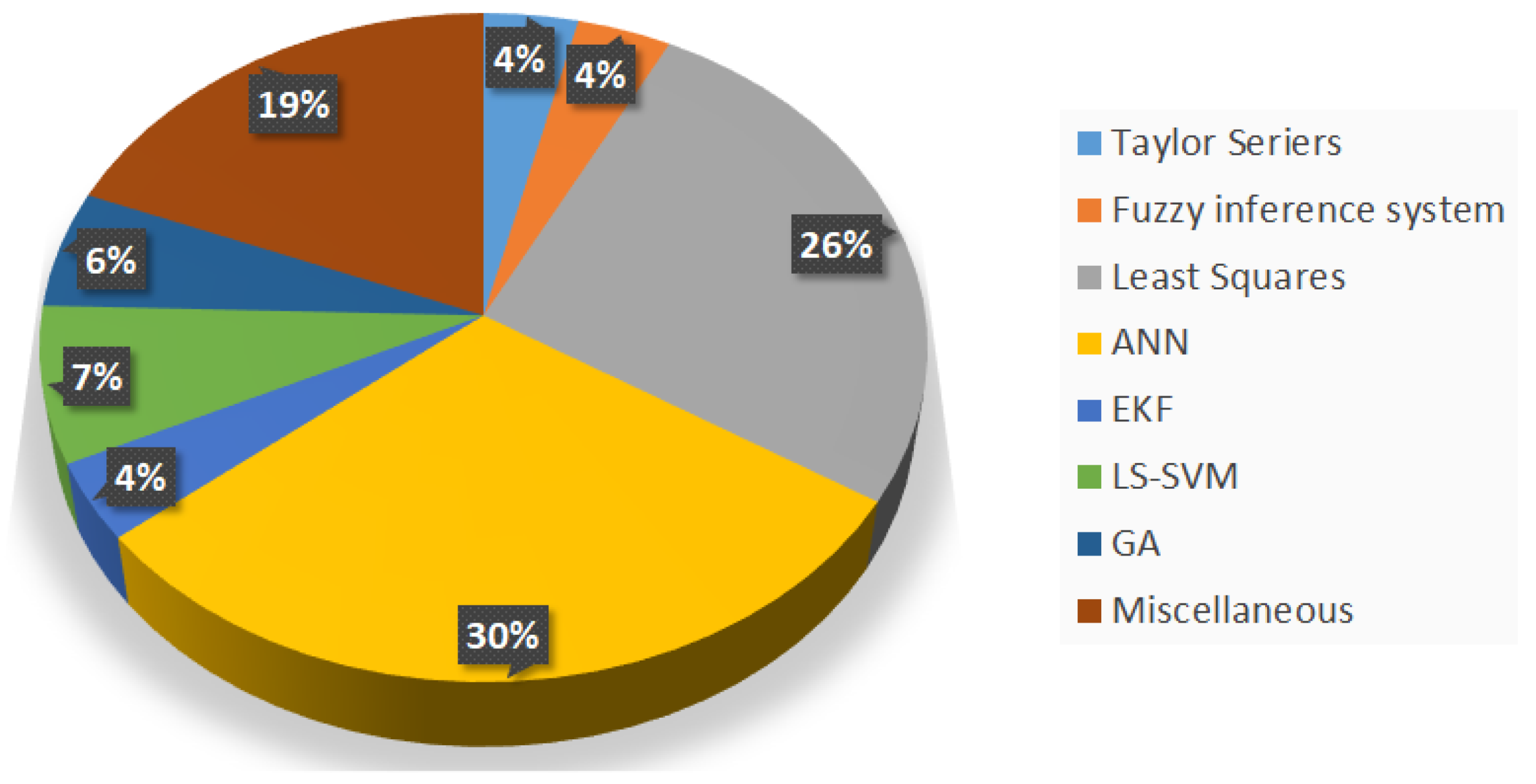
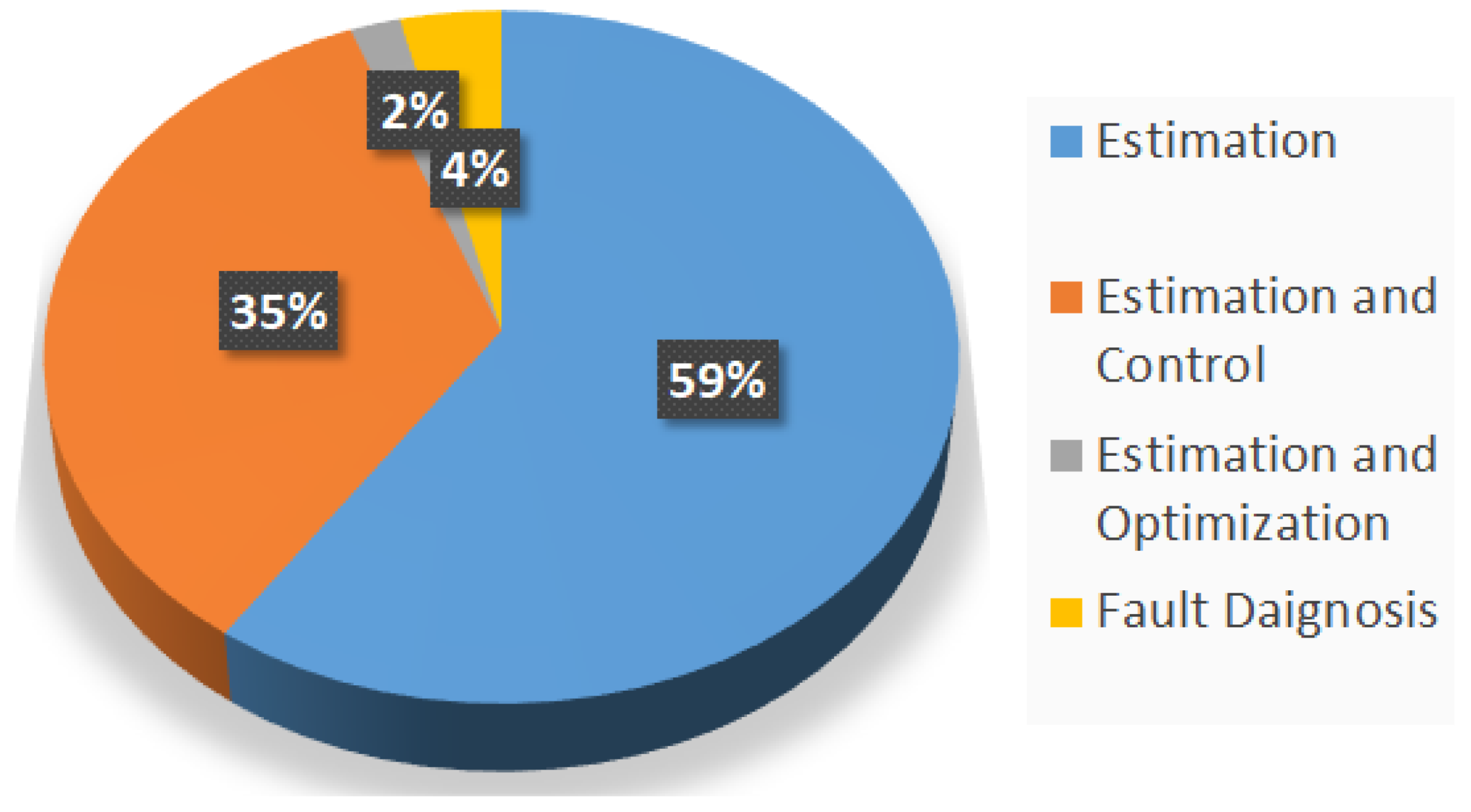
Extracts from the reviewed papers are summarized in Table 1, Table 2 and Table 3. The percentage distribution of GB models in terms of the type of process industries is shown in Figure 2. The chemical, biochemical and pharmaceutical industry collectively have a share of 20% followed by iron and steel at 11%, oil and gas processing at 9%, materials process and energy materials at 7%, industrial robots at 7%, food industry at 5%, power plants at 5%, and water treatment at 5%. The miscellaneous studies have a collective share of 31% with further breakdown into heat transfer systems at 57% followed by reactive systems at 47%. The percentage share of types of GB sensors, i.e., parallel, serial and combined, is shown in Figure 3. The serial GB models get a share of 84% followed by parallel GB at 11% and combined GB models at 2%. Of all the cases, 3% used all three types of GB models. The percentage share of BB methods used in the GB design is plotted in Figure 4. ANN and it’s variants have the highest share of 30% followed by LS methods at 26%, LS-SVM at 7%, GA at 6%, EKF at 4%, Taylor series at 4%, and fuzzy inference at 4%; other methods collectively get a share of 19% however their individual share is 1% or lesser. Percentage in terms of types of application is shown in Figure 5. Estimation (only) got the highest share of 59% followed by estimation and control at 35%, fault diagnosis at 4% and estimation and optimization at 2%.
5.11. Prospects and Challenges in Industry 4.0
The data gathered in industrial processes will exponentially increase with the emergence of IoT devices. The big data gives a challenge in the form of ‘Four Vs’: volume, velocity, variety, and veracity. The huge volume of datasets may require storing and processing capacity [23]. The speed through which data is collected by the integrated smart sensors of industry 4.0 will need infrastructural change. In addition to volume and velocity, the cyber manufacturing could generate variety of data based on monitoring different parts of the system, measure different phases of the process, which can be sampled at very different frequencies. The undesired samples collected due to the highly speedy sensors add veracity to the database. This type of data is not representative of the process and create an extremely heterogeneous data structure. In this context, outliers, missing data, noises, delays and data synchronism will need to be addressed [22]. To use the big data in process inference, i.e., monitoring, control, optimization, data processing methods need to be applied in the initial phase. These methods include data wrangling, visualization, sparsity and regularization, optimization, reducing dimensionality, measuring distance, representation learning, and sequential learning [24,25,26,27].
With the emergence of big data in the process industry, the GB model will need to be equiped for effectively dealing with the new scenario. The WB modeling part of the GB will mostly remain the same; however, the data-driven part will be affected by the massive amount of process data. In this context, several studies have been reported on soft sensor design based on big data, i.e., taken from IoT sensors, [17,18,19,20,21]. Although these studies were based on BB soft sensors, they are summarized here to understand the additional tasks in developing the BB part of the GB soft sensors in the context of the big data.
Klusch et al. [20] developed an IoT sensing system for a hydraulic aggregate consisting of an oil tank and electric motor pump. Eighteen sensors were used to monitor physical parameters such as pressure, air and oil temperature, and vibration, etc., of the oil pump in the aggregate. A stream of 50,000 data samples from 18 sensors per minute was collected. Feature reduction and annotation were performed on the basis of statistic and semantic components of the system. Then, an integration of statistical, probabilistic and semantic data analysis was used for fault detection and diagnosis of the system.
He et al. [18] developed an IoT-enabled manufacturing technology testbed (MTT) system based on temperature sensors. The sensing system comprised of 28 IoT temperature sensors attached to a CSTR plus corresponding data acquisition, transmission and storage systems. The IoT-enabled MTT made it possible to measure the real temperature distribution without assuming ideal mixing. It was observed that the IoT sensors exhibit noisy or spiky behavior at the steady state. In addition, the sensor readings fall at fixed grids and most of the IoT sensors show different levels of persistent bias. A variation in sample collection interval was also noted. Then, a statistics pattern analysis (SPA) was developed to deal with the big data related issues and effectively perform fault detection and diagnosis of the system.
Shah et al. [17] developed an IoT testbed for a multi-stage centrifugal pumping system. Non-invasive IoT vibration sensors were attached to centrifugal pumping system. The veracity of the data, i.e., unequal sampling intervals, significant noise and missing values, and its impact on data analytics was investigated. It was found that the use of Lomb’s algorithm can effectively handle the data veracity. Furthermore, they devised a method of dealing with the challenge of volume and velocity. Finally, a framework of process monitoring based on data-driven predictive models for flow rate inside the pipe and speed of the pump motor was devised.
Syafrudin et al. [19] attached IoT-based sensors to the desk of a workstation in the assembly line to sense temperature, accelerometer, humidity, and gyroscope sensors. The massive data collected through the sensors were saved in the MongoDB database. An outlier detection approach was devised using the clustering technique. Then data-based fault classification of the assembly line was developed. In addition, a history of the temperature, accelerometer, humidity, and gyroscope data were displayed to the manager in real-time via a web-based monitoring system.
6. Conclusions
GB models are developed through the integration of WB and BB models. GB models have been getting the attention of researchers due to their higher intuitiveness than the BB models and high estimation accuracy than the standalone WB models. GB models are further classified into three categories namely parallel, serial and combined GB models. In the parallel GB models, BB models are used to compensate the error of WB models of the process. In the serial GB models, BB models are used to estimate parameters of the WB model. The combined GB sensors integrate the parallel and serial GB models to realize higher prediction accuracy. Applications of GB models in the process industry have been reported in iron and steel making, food processing, power plants, chemical, biochemical, pharmaceutical, water treatment, oil and gas processing, material processing, energy materials, and industrial robot.
Chemical, biochemical and pharmaceutical industry have a collective share of 20% followed by iron and steel at 11%, oil and gas processing at 9%, materials process and energy materials at 7%, industrial robots at 7%, food industry at 5%, power plants at 5%, and water treatment at 5%. In terms of percentage share of types of GB sensors, the serial GB models got a share of 84% followed by parallel GB at 11% and combined GB models at 2%. Of all cases, 3% used all three types of GB models. In terms of percentage share of BB methods used in the GB design, ANN and it’s variants have the highest percentage share of 30% followed by LS methods at 26%, LS-SVM at 7%, GA at 6%, EKF at 4%, Taylor series at 4%, and fuzzy inference at 4%. In terms of percentage of types of application, estimation (only) got the highest share of 59% followed by estimation and control at 35%, fault diagnosis at 4%, estimation and optimization at 2%.
To use the big data in process inference, i.e., monitoring, control, optimization, data processing methods need to be applied in the initial phase before development of data-based or GB models. The data pre-processing methods include data wrangling, visualization, sparsity and regularization, optimization, reducing dimensionality, measuring distance, representation learning, and sequential learning. These data preprocessing techniques are required in realizing highly efficient BB models. However, GB models, being dependent on BB models, will also need these techniques if a GB model is to be applied to Industry 4.0.
Author Contributions
Conceptualization, I.A.; methodology, I.A.; formal analysis, I.A.; investigation, I.A.; A.A.; writing—original draft preparation, I.A.; A.A.; writing—review and editing, I.I.C.; M.K. All authors have read and agreed to the published version of the manuscript.
Funding
This research received no external funding.
Conflicts of Interest
The authors declare no conflict of interest.
Abbreviations
The following abbreviations are used in this manuscript:
| ALAMO | Automatic learning of algebraic models |
| ANN | Artificial neural network |
| ARMAX | Autoregressive moving average exogenous |
| ARXIs | Auto-regressive with exogenous |
| BB | Black-box |
| CDU | Crude distillation unit |
| CSTR | Continuous stirred tank reactor |
| DR | Data reconciliation |
| EKF | Extended Kalman Filter |
| FIS | Fuzzy inference system |
| GA | Genetic algorithm |
| GB | Gray-box |
| IoT | Internet of things |
| LS | Least squares |
| LS-SVM | Least squares support vector machine |
| MF | Membership function |
| MLE | Maximum likelihood estimation |
| MLSSVM | Multi-I/O least squares support vector machine |
| MPC | Model for predictive control |
| MTT | Manufacturing technology testbed |
| MWD | Molecular weight distribution |
| OPFNN | Orthogonal polynomial feed forward neural network |
| PCA | Principle component analysis |
| PLS | Partial least squares |
| PV | Photovoltaic |
| RF | Random forests |
| RNN | Recurrent neural network |
| RTO | Real time optimization |
| SB | Scale breaker |
| SCR | Selective catalytic reduction |
| SDEs | Stochastic differential equations |
| SDO | Simulink design optimization tool |
| SMR | Steam methane reforming |
| SPA | Statistics pattern analysis |
| SPSA | Simultaneous perturbation stochastic approximation |
| SSM | State space model |
| SVM | Support vector machine |
| TSE | Twin screw extruder |
| WB | White-box |
| WLLS | Weighted logarithmic least squares |
| WRRFs | Water resource recovery facilities |
References
- Oztemel, E.; Gursev, S. Literature review of Industry 4.0 and related technologies. J. Intell. Manuf. 2020, 31, 127–182. [Google Scholar] [CrossRef]
- Jiang, Y.; Yin, S.; Kaynak, O. Data-driven monitoring and safety control of industrial cyber-physical systems: Basics and beyond. IEEE Access 2018, 6, 47374–47384. [Google Scholar] [CrossRef]
- Joly, M.; Odloak, D.; Miyake, M.Y.; Menezes, B.C.; Kelly, J.D. Refinery production scheduling toward Industry 4.0. Front. Manag. Eng. 2017, 37, 1877–1882. [Google Scholar] [CrossRef]
- Khan, A.; Turowski, K. A Perspective on Industry 4.0: From Challenges to Opportunities in Production Systems. In Proceedings of the IoTBD, Rome, Italy, 23–25 April 2016; pp. 441–448. [Google Scholar]
- Candanedo, I.S.; Nieves, E.H.; González, S.R.; Martín, M.T.S.; Briones, A.G. Machine learning predictive model for industry 4.0. In International Conference on Knowledge Management in Organizations; Springer: Berlin, Germany, 2018; pp. 501–510. [Google Scholar]
- Zheng, P.; Wang, H.; Sang, Z.; Zhong, R.Y.; Liu, Y.; Liu, C.; Mubarok, K.; Yu, S.; Xu, X. Smart manufacturing systems for Industry 4.0: Conceptual framework, scenarios, and future perspectives. Front. Mech. Eng. 2018, 13, 137–150. [Google Scholar] [CrossRef]
- Rüßmann, M.; Lorenz, M.; Gerbert, P.; Waldner, M.; Justus, J.; Engel, P.; Harnisch, M. Industry 4.0: The future of productivity and growth in manufacturing industries. Boston Consult. Group 2015, 9, 54–89. [Google Scholar]
- Weyrich, M.; Ebert, C. Reference architectures for the internet of things. IEEE Softw. 2016, 33, 112–116. [Google Scholar] [CrossRef]
- Schütze, A.; Helwig, N.; Schneider, T. Sensors 4.0–smart sensors and measurement technology enable Industry 4.0. J. Sensors Sens. Syst. 2018, 7, 359–371. [Google Scholar] [CrossRef]
- Tameh, T.A.; Sawan, M.; Kashyap, R. Smart integrated optical rotation sensor incorporating a fly-by-wire control system. IEEE Trans. Ind. Electron. 2017, 65, 6505–6514. [Google Scholar] [CrossRef]
- Martinez-Figueroa, G.D.J.; Morinigo-Sotelo, D.; Zorita-Lamadrid, A.L.; Morales-Velazquez, L.; Romero-Troncoso, R.D.J. Fpga-based smart sensor for detection and classification of power quality disturbances using higher order statistics. IEEE Access 2017, 5, 14259–14274. [Google Scholar] [CrossRef]
- Cloete, N.A.; Malekian, R.; Nair, L. Design of smart sensors for real-time water quality monitoring. IEEE Access 2016, 4, 3975–3990. [Google Scholar] [CrossRef]
- Maciá-Pérez, F.; Mora-Gimeno, F.J.; Marcos-Jorquera, D.; Gil-Martínez-Abarca, J.A.; Ramos-Morillo, H.; Lorenzo-Fonseca, I. Network intrusion detection system embedded on a smart sensor. IEEE Trans. Ind. Electron. 2010, 58, 722–732. [Google Scholar] [CrossRef] [Green Version]
- Hu, Y.; Zhang, S.; Yan, Y.; Wang, L.; Qian, X.; Yang, L. A smart electrostatic sensor for online condition monitoring of power transmission belts. IEEE Trans. Ind. Electron. 2017, 64, 7313–7322. [Google Scholar] [CrossRef]
- Alahi, M.E.E.; Xie, L.; Mukhopadhyay, S.; Burkitt, L. A temperature compensated smart nitrate-sensor for agricultural industry. IEEE Trans. Ind. Electron. 2017, 64, 7333–7341. [Google Scholar] [CrossRef]
- Lin, F.; Wang, A.; Zhuang, Y.; Tomita, M.R.; Xu, W. Smart insole: A wearable sensor device for unobtrusive gait monitoring in daily life. IEEE Trans. Ind. Inform. 2016, 12, 2281–2291. [Google Scholar] [CrossRef]
- Shah, D.; Wang, J.; He, Q.P. An Internet-of-things Enabled Smart Manufacturing Testbed. IFAC-PapersOnLine 2019, 52, 562–567. [Google Scholar] [CrossRef]
- He, Q.P.; Wang, J.; Shah, D.; Vahdat, N. Statistical process monitoring for IoT-Enabled cybermanufacturing: opportunities and challenges. IFAC-PapersOnLine 2017, 50, 14946–14951. [Google Scholar] [CrossRef]
- Syafrudin, M.; Alfian, G.; Fitriyani, N.; Rhee, J. Performance Analysis of IoT-Based Sensor, Big Data Processing, and Machine Learning Model for Real-Time Monitoring System in Automotive Manufacturing. Sensors 2018, 18, 2946. [Google Scholar] [CrossRef] [PubMed] [Green Version]
- Klusch, M.; Meshram, A.; Schuetze, A.; Helwig, N. iCM-Hydraulic: Semantics-empowered condition monitoring of hydraulic machines. In Proceedings of the 11th International Conference on Semantic Systems, Vienna, Austria, 15–17 September 2015; pp. 81–88. [Google Scholar]
- He, Q.P.; Wang, J. Statistical process monitoring as a big data analytics tool for smart manufacturing. J. Process Control 2018, 67, 35–43. [Google Scholar] [CrossRef]
- Hodas, N.O.; Lerman, K. The simple rules of social contagion. Sci. Rep. 2014, 4, 4343. [Google Scholar] [CrossRef] [Green Version]
- Shvachko, K.; Kuang, H.; Radia, S.; Chansler, R. The hadoop distributed file system. In Proceedings of the MSST, Incline Village, NV, USA, 3–7 May 2010; Volume 10, pp. 1–10. [Google Scholar]
- Bengio, Y.; Courville, A.; Vincent, P. Representation learning: A review and new perspectives. IEEE Trans. Pattern Anal. Mach. Intell. 2013, 35, 1798–1828. [Google Scholar] [CrossRef]
- Anandkumar, A.; Hsu, D.J.; Janzamin, M.; Kakade, S.M. When are overcomplete topic models identifiable? uniqueness of tensor tucker decompositions with structured sparsity. In Advances in Neural Information Processing Systems 26; Curran Associates, Inc.: Red Hook, NY, USA, 2013; pp. 1986–1994. [Google Scholar]
- Kalal, Z.; Mikolajczyk, K.; Matas, J. Tracking-learning-detection. IEEE Trans. Pattern Anal. Mach. Intell. 2011, 34, 1409–1422. [Google Scholar] [CrossRef] [PubMed] [Green Version]
- Scott, S.L.; Blocker, A.W.; Bonassi, F.V.; Chipman, H.A.; George, E.I.; McCulloch, R.E. Bayes and big data: The consensus Monte Carlo algorithm. Int. J. Manag. Sci. Eng. Manag. 2016, 11, 78–88. [Google Scholar] [CrossRef] [Green Version]
- Kadlec, P.; Gabrys, B.; Strandt, S. Data-driven soft sensors in the process industry. Comput. Chem. Eng. 2009, 33, 795–814. [Google Scholar] [CrossRef] [Green Version]
- Kano, M.; Fujiwara, K. Virtual sensing technology in process industries: Trends and challenges revealed by recent industrial applications. J. Chem. Eng. Jpn. 2013, 46, 1–17. [Google Scholar] [CrossRef] [Green Version]
- Kaneko, H.; Arakawa, M.; Funatsu, K. Development of a new soft sensor method using independent component analysis and partial least squares. AIChE J. 2009, 55, 87–98. [Google Scholar] [CrossRef]
- Sun, K.; Liu, J.; Kang, J.L.; Jang, S.S.; Wong, D.S.H.; Chen, D.S. Soft Sensor Development with Nonlinear Variable Selection Using Nonnegative Garrote and Artificial Neural Network. In Computer Aided Chemical Engineering; Elsevier: Amsterdam, The Netherlands, 2014; Volume 33, pp. 883–888. [Google Scholar]
- Sohlberg, B. Hybrid grey box modelling of a pickling process. Control Eng. Pract. 2005, 13, 1093–1102. [Google Scholar] [CrossRef]
- Barrios, J.A.; Cavazos, A.; Leduc, L.; Ramírez, J. Fuzzy and fuzzy grey-box modelling for entry temperature prediction in a hot strip mill. Mater. Manuf. Process. 2011, 26, 66–77. [Google Scholar] [CrossRef]
- Ahmad, I.; Kano, M.; Hasebe, S.; Kitada, H.; Murata, N. Gray-box modeling for prediction and control of molten steel temperature in tundish. J. Process Control 2014, 24, 375–382. [Google Scholar] [CrossRef] [Green Version]
- Ahmad, I.; Kano, M.; Hasebe, S.; Kitada, H.; Murata, N. Prediction of molten steel temperature in steel making process with uncertainty by integrating gray-box model and bootstrap filter. J. Chem. Eng. Jpn. 2014, 47, 827–834. [Google Scholar] [CrossRef] [Green Version]
- Barrios, J.A.; Torres-Alvarado, M.; Cavazos, A.; Leduc, L. Neural and Neural Gray-Box modeling for entry temperature prediction in a hot strip mill. J. Mater. Eng. Perform. 2011, 20, 1128–1139. [Google Scholar] [CrossRef]
- Cubillos, F.A.; Vyhmeister, E.; Acuña, G.; Alvarez, P.I. Rotary dryer control using a grey-box neural model scheme. Dry. Technol. 2011, 29, 1820–1827. [Google Scholar] [CrossRef]
- Vieira, G.N.A.; Freire, F.B.; Freire, J.T. Control of the moisture content of milk powder produced in a spouted bed dryer using a grey-box inferential controller. Dry. Technol. 2015, 33, 1920–1928. [Google Scholar] [CrossRef]
- Saltık, M.B.; Özkan, L.; Jacobs, M.; van der Padt, A. Dynamic modeling of ultrafiltration membranes for whey separation processes. Comput. Chem. Eng. 2017, 99, 280–295. [Google Scholar] [CrossRef]
- Møller, J.K.; Goranović, G.; Poulsen, N.K.; Madsen, H. Physical-stochastic (greybox) modeling of slugging. Ifac-Papersonline 2018, 51, 197–202. [Google Scholar] [CrossRef]
- Onel, O.; Niziolek, A.M.; Butcher, H.; Wilhite, B.A.; Floudas, C.A. Multi-scale approaches for gas-to-liquids process intensification: CFD modeling, process synthesis, and global optimization. Comput. Chem. Eng. 2017, 105, 276–296. [Google Scholar] [CrossRef]
- Bram, M.V.; Hansen, L.; Hansen, D.S.; Yang, Z. Grey-Box modeling of an offshore deoiling hydrocyclone system. In Proceedings of the 2017 IEEE Conference on Control Technology and Applications (CCTA), Mauna Lani, HI, USA, 27–30 August 2017; pp. 94–98. [Google Scholar]
- Lotfalipour, M.R.; Falahi, M.A.; Bastam, M. Prediction of CO2 emissions in Iran using grey and ARIMA models. Int. J. Energy Econ. Policy 2013, 3, 229–237. [Google Scholar]
- Durrani, M.; Ahmad, I.; Kano, M.; Hasebe, S. An Artificial Intelligence Method for Energy Efficient Operation of Crude Distillation Units under Uncertain Feed Composition. Energies 2018, 11, 2993. [Google Scholar] [CrossRef] [Green Version]
- Prada Moraga, C.D.; Hose, D.; Gutierrez, G.; Pitarch, J.L. Developing Grey-Box Dynamic Process Models. IFAC-PapersOnLine 2013, 51, 523–528. [Google Scholar] [CrossRef]
- Wang, B.; Yu, M.; Zhu, X.; Zhu, L.; Jiang, Z. A Robust Decoupling Control Method Based on Artificial Bee Colony-Multiple Least Squares Support Vector Machine Inversion for Marine Alkaline Protease MP Fermentation Process. IEEE Access 2019, 7, 32206–32216. [Google Scholar] [CrossRef]
- Niu, D.; Jia, M.; Wang, F.; He, D. Optimization of nosiheptide fed-batch fermentation process based on hybrid model. Ind. Eng. Chem. Res. 2013, 52, 3373–3380. [Google Scholar] [CrossRef]
- Johansen, T.A.; Foss, B.A. Representing and learning unmodeled dynamics with neural network memories. In Proceedings of the American Control Conference, Chicago, IL, USA, 24–26 June 1992; pp. 3037–3043. [Google Scholar]
- Liu, X.; Li, K.; McAfee, M.; Nguyen, B.K.; McNally, G.M. Dynamic gray-box modeling for on-line monitoring of polymer extrusion viscosity. Polym. Eng. Sci. 2012, 52, 1332–1341. [Google Scholar] [CrossRef] [Green Version]
- Everett, S.E.; Dubay, R. A sub-space artificial neural network for mold cooling in injection molding. Expert Syst. Appl. 2017, 79, 358–371. [Google Scholar] [CrossRef]
- Zahedi, G.; Azizia, S.; Hatamia, T.; Sheikhattar, L. Gray box modeling of supercritical nimbin extraction from neem seeds using methanol as co-solvent. Open Chem. Eng. J. 2010, 4, 21–30. [Google Scholar] [CrossRef] [Green Version]
- Cubillos, F.; Acuña, G.; Lima, E. Real-time process optimization based on grey-box neural models. Braz. J. Chem. Eng. 2007, 24, 433–443. [Google Scholar] [CrossRef] [Green Version]
- Pitarch, J.L.; Sala, A.; de Prada, C. A Systematic Grey-Box Modeling Methodology via Data Reconciliation and SOS Constrained Regression. Processes 2019, 7, 170. [Google Scholar] [CrossRef] [Green Version]
- Liu, G.; Yu, S.; Mei, C.; Ding, Y. A novel soft sensor model based on artificial neural network in the fermentation process. Afr. J. Biotechnol. 2011, 10, 19780–19787. [Google Scholar]
- Zhao, H.; Shen, J.; Li, Y.; Bentsman, J. Coal-fired utility boiler modelling for advanced economical low-NOx combustion controller design. Control Eng. Pract. 2017, 58, 127–141. [Google Scholar] [CrossRef]
- Arahal, M.R.; Cirre, C.M.; Berenguel, M. Serial grey-box model of a stratified thermal tank for hierarchical control of a solar plant. Sol. Energy 2008, 82, 441–451. [Google Scholar] [CrossRef]
- Barszcz, T.; Czop, P. Estimation of feedwater heater parameters based on a grey-box approach. Int. J. Appl. Math. Comput. Sci. 2011, 21, 703–715. [Google Scholar] [CrossRef]
- Stentoft, P.A.; Guericke, D.; Munk-Nielsen, T.; Mikkelsen, P.S.; Madsen, H.; Vezzaro, L.; Møller, J.K. Model Predictive Control of Stochastic Wastewater Treatment Process for Smart Power, Cost-Effective Aeration. In Proceedings of the 12th IFAC Symposium on Dynamics and Control of Process Systems, Florianópolis, Brazil, 23–26 April 2019. [Google Scholar]
- Stentoft, P.A.; Munk-Nielsen, T.; Vezzaro, L.; Madsen, H.; Mikkelsen, P.S.; Møller, J.K. Towards model predictive control: Online predictions of ammonium and nitrate removal by using a stochastic ASM. Water Sci. Technol. 2019, 79, 51–62. [Google Scholar] [CrossRef] [PubMed] [Green Version]
- Dragoi, E.N.; Horoba, C.A.; Mamaliga, I.; Curteanu, S. Grey and black-box modelling based on neural networks and artificial immune systems applied to solid dissolution by rotating disc method. Chem. Eng. Process. Process Intensif. 2014, 82, 173–184. [Google Scholar] [CrossRef]
- Li, D.C.; Yeh, C.W.; Chen, C.C.; Wang, Y.T. A new grey prediction model for the return material authorization process in the TFT-LCD industry. Int. J. Adv. Manuf. Technol. 2018, 96, 2149–2160. [Google Scholar] [CrossRef]
- Rad, C.R.; Hancu, O.; Lapusan, C. Gray-box modeling and closed-loop temperature control of a thermotronic system. In Proceedings of the 11th IFToMM International Symposium on Science of Mechanisms and Machines, Braşov, Romania, 11–12 November 2013; Springer: Cham, Switzerland, 2014; pp. 197–207. [Google Scholar]
- Masoudinejad, M.; Kamat, M.; Emmerich, J.; ten Hompel, M.; Sardesai, S. A gray box modeling of a photovoltaic cell under low illumination in materials handling application. In Proceedings of the 2015 3rd International Renewable and Sustainable Energy Conference (IRSEC), Marrakech, Morocco, 10–13 December 2015; pp. 1–6. [Google Scholar]
- Liu, G.; Dass, R.; Nguang, S.K.; Partridge, A. Principles, design, and calibration for a genre of irradiation angle sensors. IEEE Trans. Ind. Electron. 2012, 60, 210–216. [Google Scholar] [CrossRef]
- Wernholt, E.; Moberg, S. Frequency-domain gray-box identification of industrial robots. IFAC Proc. Vol. 2008, 41, 15372–15380. [Google Scholar] [CrossRef] [Green Version]
- Ayala, H.V.H.; Habineza, D.; Rakotondrabe, M.; Klein, C.E.; Coelho, L.S. Nonlinear black-box system identification through neural networks of a hysteretic piezoelectric robotic micromanipulator. IFAC-PapersOnLine 2015, 48, 409–414. [Google Scholar] [CrossRef]
- Wernholt, E.; Moberg, S. Nonlinear gray-box identification using local models applied to industrial robots. Automatica 2011, 47, 650–660. [Google Scholar] [CrossRef] [Green Version]
- Zendehboudi, S.; Rezaei, N.; Lohi, A. Applications of hybrid models in chemical, petroleum, and energy systems: A systematic review. Appl. Energy 2018, 228, 2539–2566. [Google Scholar] [CrossRef]
- Wu, Z.; Li, J.; Cai, M.; Lin, Y.; Zhang, W. On membership of black-box or white-box of artificial neural network models. In Proceedings of the 12016 IEEE 11th Conference on Industrial Electronics and Applications (ICIEA), Hefei, China, 5–7 June 2016; pp. 1400–1404. [Google Scholar]
- Hangos, K.M.; Cameron, I.T. Process modelling and model analysis; Academic Press: London, UK, 2001; Volume 4. [Google Scholar]
- Jin, C.; Cusatis, G. New Frontiers in Oil and Gas Exploration; Springer: Berlin, Germany, 2016. [Google Scholar]
- Nelles, O. Nonlinear System Identification: From Classical Approaches to Neural Networks and Fuzzy Models; Springer Science & Business Media: Berin/Hedelberg, Germany, 2013. [Google Scholar]
- Grossmann, I.E.; Westerberg, A.W. Research challenges in process systems engineering. AIChE J. 2000, 46, 1700–1703. [Google Scholar] [CrossRef]
- Chaves, I.D.G.; López, J.R.G.; Zapata, J.L.G.; Robayo, A.L.; Niño, G.R. Process Analysis and Simulation in Chemical Engineering; Springer: Berlin, Germany, 2016. [Google Scholar]
- Bequette, B.W. Nonlinear control of chemical processes: A review. Ind. Eng. Chem. Res. 1991, 30, 1391–1413. [Google Scholar] [CrossRef]
- Guay, M.; McLellan, P.; Bacon, D. Measurement of nonlinearity in chemical process control systems: The steady state map. Can. J. Chem. Eng. 1995, 73, 868–882. [Google Scholar] [CrossRef]
- Krasławski, A. Review of applications of various types of uncertainty in chemical engineering. Chem. Eng. Process. Process Intensif. 1989, 26, 185–191. [Google Scholar] [CrossRef]
- Ahmad, I.; Kano, M.; Hasebe, S. Dimensions and analysis of uncertainty in industrial modeling process. J. Chem. Eng. Jpn. 2018, 51, 533–543. [Google Scholar] [CrossRef]
- Li, J.; Kwauk, M. Exploring complex systems in chemical engineering—the multi-scale methodology. Chem. Eng. Sci. 2003, 58, 521–535. [Google Scholar] [CrossRef]
- Li, G.; Rosenthal, C.; Rabitz, H. High dimensional model representations. J. Phys. Chem. A 2001, 105, 7765–7777. [Google Scholar] [CrossRef]
- Michiels, W.; Niculescu, S.I. Stability, Control, and Computation for Time-Delay Systems: An Eigenvalue-Based Approach; Siam: Philadelphia, PA, USA , 2014; Volume 27. [Google Scholar]
- Cherkassky, V.; Mulier, F.M. Learning from Data: Concepts, Theory, and Methods; John Wiley & Sons: Hoboken, NJ, USA, 2007. [Google Scholar]
- Mokhatab, S.; Poe, W.A. Handbook of Natural Gas Transmission and Processing; Gulf professional publishing: Houston, TX, USA, 2012. [Google Scholar]
- Jank, B. Instrumentation, Control and Automation of Water and Wastewater Treatment and Transport Systems 1993; Elsevier: Amsterdam, The Netherlands, 2016. [Google Scholar]
- Sjöberg, J.; Zhang, Q.; Ljung, L.; Benveniste, A.; Delyon, B.; Glorennec, P.Y.; Hjalmarsson, H.; Juditsky, A. Nonlinear black-box modeling in system identification: A unified overview. Automatica 1995, 31, 1691–1724. [Google Scholar] [CrossRef] [Green Version]
- Suykens, J.A.; Vandewalle, J.P. Nonlinear Modeling: Advanced Black-Box Techniques; Springer Science & Business Media: Berin/Hedelberg, Germany, 2012. [Google Scholar]
- Bohlin, T.; Graebe, S.F. Issues in nonlinear stochastic grey box identification. Int. J. Adapt. Control Signal Process. 1995, 9, 465–490. [Google Scholar] [CrossRef]
- Jørgensen, S.B.; Hangos, K.M. Grey box modelling for control: Qualitative models as a unifying framework. Int. J. Adapt. Control Signal Process. 1995, 9, 547–562. [Google Scholar] [CrossRef]
- Tulleken, H.J. Grey-box modelling and identification using physical knowledge and Bayesian techniques. Automatica 1993, 29, 285–308. [Google Scholar] [CrossRef]
- Bohlin, T.P. Practical Grey-Box Process Identification: Theory and Applications; Springer Science & Business Media: Berin/Hedelberg, Germany, 2006. [Google Scholar]
- Bohlin, T. Interactive system identification: Prospects and pitfalls; Springer Science & Business Media: Berin/Hedelberg, Germany, 2013. [Google Scholar]
- Okura, T.; Ahmad, I.; Kano, M.; Hasebe, S.; Kitada, H.; Murata, N. High-performance prediction of molten steel temperature in tundish through gray-box model. ISIJ Int. 2013, 53, 76–80. [Google Scholar] [CrossRef] [Green Version]
- Wu, H.; Cao, L.; Wang, J. Gray-box modeling and control of polymer molecular weight distribution using orthogonal polynomial neural networks. J. Process Control 2012, 22, 1624–1636. [Google Scholar] [CrossRef]
- Knoblach, A.; Saupe, F. LPV gray box identification of industrial robots for control. In Proceedings of the 2012 IEEE International Conference on Control Applications, Dubrovnik, Croatia, 3–5 October 2012; pp. 831–836. [Google Scholar]
- Acuña, G.; Curilem, M. Time-variant parameter estimation using a SVM Gray-Box model: Application to a CSTR Process. In Proceedings of the 3rd International Conference on Systems and Control, Algiers, Algeria, 29–31 October 2013; pp. 414–418. [Google Scholar]
- Acuña, G.; Möller, H. Indirect training of Gray-Box Models using LS-SVM and genetic algorithms. In Proceedings of the 2016 IEEE Latin American Conference on Computational Intelligence (LA-CCI), Cartagena, Colombia, 2–4 November 2016; pp. 1–5. [Google Scholar]
- Porru, G.; Aragonese, C.; Baratti, R.; Servida, A. Monitoring of a CO oxidation reactor through a grey model-based EKF observer. Chem. Eng. Sci. 2000, 55, 331–338. [Google Scholar] [CrossRef] [Green Version]
- Xiong, Q.; Jutan, A. Grey-box modelling and control of chemical processes. Chem. Eng. Sci. 2002, 57, 1027–1039. [Google Scholar] [CrossRef]
- Hourfar, F.; Salahshoor, K. Adaptive Control of CSTR Using Feedback Linearization Based on Grey-Box Modeling. In Proceedings of the IEEE International Conference on Networking, Sensing and Control, ICNSC 2008, Sanya, China, 6–8 April 2008; pp. 7–12. [Google Scholar]
- Zanardo, G.; Stadlbauer, S.; Waschl, H.; del Re, L. Grey Box Control Oriented SCR Model. In Proceedings of the 11th International Conference on Engines & Vechicles: ICE 2013, Napoli, Italy, 15–19 September 2013. [Google Scholar]
- Acuña, G.; Pinto, E. Development of a Matlab (R) Toolbox for the Design of Grey-Box Neural Models. Int. J. Comput. Commun. Control 2006, 1, 7–14. [Google Scholar] [CrossRef] [Green Version]
- Barkman, P. Grey-Box Modelling of Distributed Parameter Systems. Master’s Thesis, KTH Royal Institute of Technology, Stockholm, Sweden, 2018. [Google Scholar]
- Pearson, R.K.; Pottmann, M. Gray-box identification of block-oriented nonlinear models. J. Process Control 2000, 10, 301–315. [Google Scholar] [CrossRef]
- Weyer, E.; Szederkényi, G.; Hangos, K. Grey box fault detection of heat exchangers. Control Eng. Pract. 2000, 8, 121–131. [Google Scholar] [CrossRef]
- Miao, Q.; You, S.; Zheng, W.; Zheng, X.; Zhang, H.; Wang, Y. A Grey-Box Dynamic Model of Plate Heat Exchangers Used in an Urban Heating System. Energies 2017, 10, 1398. [Google Scholar] [CrossRef] [Green Version]
- Cubillos, F.A.; Acuña, G. Adaptive control using a grey box neural model: An experimental application. In International Symposium on Neural Networks; Springer: Berlin, Germany, 2007; pp. 311–318. [Google Scholar]
- Farooq, A.A.; Afram, A.; Schulz, N.; Janabi-Sharifi, F. Grey-box modeling of a low pressure electric boiler for domestic hot water system. Appl. Therm. Eng. 2015, 84, 257–267. [Google Scholar] [CrossRef]
- Aprile, M.; Scoccia, R.; Toppi, T.; Motta, M. Gray-box entropy-based model of a water-source NH3-H2O gas-driven absorption heat pump. Appl. Therm. Eng. 2017, 118, 214–223. [Google Scholar] [CrossRef]
- Sossan, F.; Lakshmanan, V.; Costanzo, G.T.; Marinelli, M.; Douglass, P.J.; Bindner, H. Grey-box modelling of a household refrigeration unit using time series data in application to demand side management. Sustain. Energy Grids Netw. 2016, 5, 1–12. [Google Scholar] [CrossRef] [Green Version]
- Petersen, L.N.; Poulsen, N.K.; Niemann, H.H.; Utzen, C.; Jørgensen, J.B. A grey-box model for spray drying plants. IFAC Proc. Vol. 2013, 46, 559–564. [Google Scholar] [CrossRef]
- De Moor, M.; Berckmans, D. Building a grey box model to model the energy and mass transfer in an imperfectly mixed fluid by using experimental data. Math. Comput. Simul. 1996, 42, 233–244. [Google Scholar] [CrossRef]
Figure 1.
Generalized framework grey-box (GB) modeling [34].
Figure 1.
Generalized framework grey-box (GB) modeling [34].

Figure 2.
GB models in process industries in term of percentage share; (a) collective, (b) miscellaneous.
Figure 2.
GB models in process industries in term of percentage share; (a) collective, (b) miscellaneous.

Figure 3.
Percentage share of types of GB sensors, i.e., parallel, serial and combined.

Figure 4.
Percentage share of black-box (BB) methods used in the GB design.

Figure 5.
Percentage in terms of types of application.


Table 1.
GB models application in iron and steel, food processing, chemical, biochemical, and pharmaceutical industries.
Table 1.
GB models application in iron and steel, food processing, chemical, biochemical, and pharmaceutical industries.
| Paper | Industry | Application Category | Process | GB Type | Target | BB Type |
|---|---|---|---|---|---|---|
| [32,33,34,35,36,92] | Iron and steelmaking | estimation and control | “pickling process”, “continuous casting”, “hot strip mill” | “serial”, “parallel”, “combined” | “concentration of hydrochloric acid”, “tundish temperature”, “scale breaker entry temperature”, “drying rate” | “Taylor series”, “PLS and RF”, “ANN” |
| [37,38,39] | Food industry | estimation and control | ‘fish drying process”, “milk drying process”, “whey separation” | serial | “drying rate”, “moisture contents”, “membrane fouling” | “ANN”, “exponential static membrane resistance function” |
| [45,46,47,48,49,50,51,52,53,54,93] | Chemical, biochemical, and pharmaceutical | “estimation and optimization”, “estimation and control” | “fermentation extraction”, “twin screw extruder ”, “extrusion”, “mold cooling”, “acetone-butanol ethanol fermentation process”, “MP fermentation”, “fed-batch fermentation”, “evaporation plant” | “serial”, “parallel” | “mycelia concentration”, “sugar concentration and chemical potency”, “growth rate”, “biomass concentration”, “substrate concentration and relative enzyme activity”, “substrate concentration and product concentration”, “polymerization”, “extraction yield”, “heat-transfer coefficient”, “die melting temperature”, “melt viscosity”, “cavity temperature profile” | “ARMAX”, “GA”, “ANN”, “ALAMO”, “MLSSVM integrated with artificial bee colony optimization algorithm”, “LS-SVM”, “neuro fuzzy network”, “SOS constrained polynomial regression” |
Table 2.
GB modeling application in power plant, oil and gas industry, waste water treatment, and material process and energy materials.
Table 2.
GB modeling application in power plant, oil and gas industry, waste water treatment, and material process and energy materials.
| Paper | Industry | Application Category | Process | GB Type | Target | BB Type |
|---|---|---|---|---|---|---|
| [55,56,57] | Power plant | estimation and control | “thermal storage tank”, “feed water heater/ heat exchanger” | serial | “temperature profile and the usable energy stored”, “anomaly identification”, “irradiation angle” | “simultaneous perturbation stochastic approximation”, “ANN”, “fast recursive algorithm” |
| [40,41,42,43,44] | Oil and gas processing | “estimation and control”, “estimation”, “estimation and optimization” | “CDU”, “plant wide”, “hydrocyclone system”, “valve”, “gas-to-liquids processes” | serial | “energy consumption per unit production of diesel”, “CO2 emission”, “flowrate”, “slugging”, “reactor output composition” | “ANN and GA”, “LS cost function”, “EKF”, “non-linear fitting model” |
| [58,59,60] | Water treatment | estimation and control | aeration tank | “serial”, “parallel”, “combined” | “ammonium and nitrate concentration”, “dissolution rate” | “EKF”, “ANN” |
| [61,62,63,64] | Material processing and energy materials | estimation and control | “return materials authorization process”, “thermotronic system”, “photo-voltaic cell” | serial | temperature | “fuzzy membership function”, “SDO”, “LS” |
Table 3.
GB modeling application in industrial robots and miscellaneous cases.
| Paper | Industry | Application Category | Process | GB Type | Target | BB Type |
|---|---|---|---|---|---|---|
| [65,66,67] | Industrial robot | estimation and control | process automation | serial | “motor angular speed”, “deflection of a piezoelectric micromanipulator”, “machine position” | “weighted logarithmic least squares”, “ANN”, “weighted nonlinear least squares and weighted logarithmic least squares” |
| [95,96,97,98,99,100,101,102] | Miscellaneous | estimation and control | “reactive systems” | “serial”, “paralel” | “reacytion rate”, “product composition”, “heat released”, “design of CSTR”, “concentration distributions in the context of modelling a reaction-advection-diffusion system” | “LS-SVM”, “ANN and EKF”, “ARXIs”, |
| [103,104,105,106,107,108,109,110,111] | Miscellaneous | estmation and control | heat treatment process | serial | “heat release inside the reactor”, “settled material breaking away from the heat transfer surface”, “outlet temperatures of plate heat exchangers”, “temperature of combustion chamber”, “boiler temperature”, “electricity consumption of a refrigeration system”, “spray dryer performance”, “temperature within an imperfectly mixed fluid” | “LS”, “recursive least squares identification”, “taylor series”, “ANN”, “nonlinear least squares optimization”, “linear interpolation”, “MLE” |
© 2020 by the authors. Licensee MDPI, Basel, Switzerland. This article is an open access article distributed under the terms and conditions of the Creative Commons Attribution (CC BY) license (http://creativecommons.org/licenses/by/4.0/).
Share and Cite
MDPI and ACS Style
Ahmad, I.; Ayub, A.; Kano, M.; Cheema, I.I. Gray-box Soft Sensors in Process Industry: Current Practice, and Future Prospects in Era of Big Data. Processes 2020, 8, 243. https://0-doi-org.brum.beds.ac.uk/10.3390/pr8020243
AMA Style
Ahmad I, Ayub A, Kano M, Cheema II. Gray-box Soft Sensors in Process Industry: Current Practice, and Future Prospects in Era of Big Data. Processes. 2020; 8(2):243. https://0-doi-org.brum.beds.ac.uk/10.3390/pr8020243
Chicago/Turabian StyleAhmad, Iftikhar, Ahsan Ayub, Manabu Kano, and Izzat Iqbal Cheema. 2020. "Gray-box Soft Sensors in Process Industry: Current Practice, and Future Prospects in Era of Big Data" Processes 8, no. 2: 243. https://0-doi-org.brum.beds.ac.uk/10.3390/pr8020243
Note that from the first issue of 2016, this journal uses article numbers instead of page numbers. See further details here.