Collaborative Control Applied to BSM1 for Wastewater Treatment Plants
by
 , , and
Keidy Morales-Rodelo
1,*, 
Mario Francisco
1,
Hernan Alvarez
2,
Pastora Vega
1 and
and
Silvana Revollar
1,* 1
Process Supervision and Control Research Group, Departamento de Informática y Automática, Facultad de Ciencias, Universidad de Salamanca, 37008 Salamanca, Spain
2
Kalman Research Group, Departamento de Procesos y Energía, Facultad de Minas, Universidad Nacional de Colombia, Medellín 050041, Colombia
*
Authors to whom correspondence should be addressed.
Processes 2020, 8(11), 1465; https://0-doi-org.brum.beds.ac.uk/10.3390/pr8111465
Submission received: 12 October 2020
/
Revised: 5 November 2020
/
Accepted: 11 November 2020
/
Published: 16 November 2020
(This article belongs to the Section Process Control and Monitoring)
Abstract
:This paper describes a design procedure for a collaborative control structure in Plant Wide Control (PWC), taking into account the existing controllable parameters as a novelty in the procedure. The collaborative control structure includes two layers, supervisory and regulatory, which are determined according to the dynamics hierarchy obtained by means of the Hankel matrix. The supervisory layer is determined by the main dynamics of the process and the regulatory layer comprises the secondary dynamics and controllable parameters. The methodology proposed is applied to a wastewater treatment plant, particularly to the Benchmark Simulation Model No 1 (BSM1) for the activated sludge process, comparing the results with the use of a Model Predictive Controller in the supervisory layer. For determining controllable parameters in the BSM1 control, a new specific oxygen mass transfer model in the biological reactor has been developed, separating the volumetric mass transfer coefficient into two controllable parameters, and a.
1. Introduction
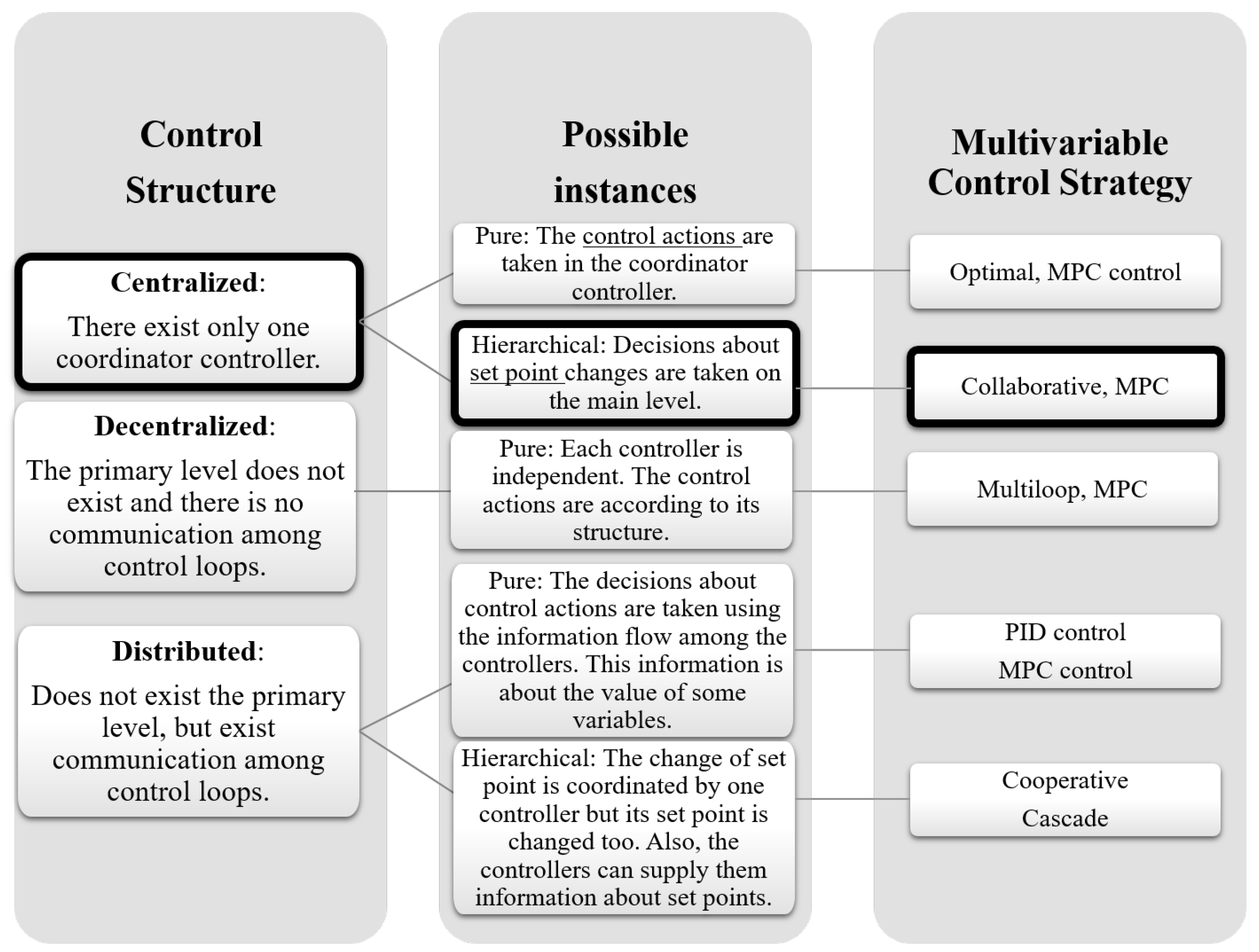
The plantwide control (PWC) approach is the most widely used solution for optimization and control of large-scale processes. This methodology provides a link between the systems and strategies necessary to control a large scale chemical plant comprised by different interacting units [1]. PWC has been a very active research field due to the significant improvements to the operation of industrial processes [2]. There are different approaches, broadly classified in centralized, decentralized, and distributed control. In Figure 1, a general arrangement for PWC methodologies is presented, and more details are given in [3].
The simplest approach is a centralized control structure, where a unique coordinator controller either selects the set points for other controllers in the lower layer or sends information directly to the final control elements (FCE) [4]. In a hierarchical structure, the coordinator controller is typically an optimization based controller, and PID controllers are in the lower level, which focuses on plant behavior and its dynamic interactions [5,6]. The optimization based controller can be an economic one including costs in the objective function, or a standard Model-based predictive controller (MPC). The lower level typically consists of several independent PID control loops but multiple MPC control loops can also be considered. Model-based predictive control (MPC) is a powerful strategy frequently used in Decentralized and Distributed control structures. The MPC algorithm performs an optimization at each sampling time to obtain the optimal values of the manipulated inputs [7]. This advanced control strategy considers an objective function that includes tracking errors and control efforts properly balanced and constraints on control and input variables in the formulation of the optimization problem.
Despite of the large amount of MPC successful applications, especially in the process industries [8], they have some drawbacks, such as the computational load required to solve the optimization problems involved, in particular when the prediction model is nonlinear. Another drawback is the difficulty for tuning the controller parameters, which is often performed by a trial and error procedure. Therefore, in this work, collaborative control is proposed as a practical multivariable control strategy for implementing a hierarchical centralized control structure, and it is compared to the use of MPC as an alternative strategy. In this strategy, the key point is the determination of a dynamics hierarchy using the Hankel matrix that gives the impact of the inputs on the plant states. The main dynamics is located in the upper layer and the rest of control handles can be used as collaborative regulatory controllers aiming to achieve the global objective. Collaborative characteristics imply a direct relation among all secondary dynamics and main dynamics in order to regulate the main dynamic, unlike in common MPC strategies.
Therefore, two levels are considered in the collaborative hierarchical structure: a supervisory layer where the coordinator controller provides set points for the regulatory layer [5], and the regulatory layer comprised by the controllers receiving this information. Usually, local PID controllers are employed in the lower level, each one associated with one process unit. However, it is important to highlight that collaborative control is different from cooperative control. Collaboration occurs when individuals from different species work together for a common goal, while cooperation concept implies that individuals from the same species are working for the same objective. Thus, the conditions for the implementation of collaborative control strategies are commonly found in chemical processes, where each subsystem (e.g., reaction units, separation processes, transportation) pursues a common objective, the final product, even though dynamics of the different subsystems are different (e.g., temperature, concentration, level). On the other hand, classic examples of cooperative control are found in robotics applications, where a team of robots with similar characteristics work for a common goal.
The concept of collaboration is considered in different fields of knowledge. The measurement of collaborative intelligence in knowledge based service planning is studied in [9] who identify measures to achieve the best collaboration between different enterprises. The application of collaborative control in a robotic wheelchair is addressed in [10] introducing a collaborative control mechanism that assists users when they require some help. In [11], a collaborative control strategy is used for teleoperation systems, where the human is modeled as a collaborator in a multidisciplinary team. They say that in “collaborative control model a human operator and a robot are peers who work together, collaborating to perform tasks and to achieve common goals”.
Although few applications of collaborative control in chemical processes are found, some works have employed this strategy for hierarchical control with good results. In [12], a multilayer architecture is considered to control a continuous bioethanol process. They use two kinds of PWC schemes and compare single layer with multilayer structures. In [6], a collaborative control structure with communication between the process units and a coordinator controller is presented. In this methodology, the Hankel matrix is used to classify the different dynamics. Similar approaches can be found in [12,13,14]. The works of [15,16,17] explore the possibility of introducing some kind of sensitivity terms in the objective function for the optimization of large-scale process. Although all these works demonstrate the potential of collaborative control strategy, some further improvement could be achieved including controllable parameters in the control structure.
The main contribution of the collaborative control strategy proposed in this work is the possibility of exploiting the manipulation of some process parameters to improve the overall process performance. The capabilities of the collaborative control strategy are improved introducing one or more process controllable parameters into the strategy as additional control handles. Another contribution of this work is the application of this methodology to wastewater treatment plants (WWTP), especially to the activated sludge process. The Benchmark Simulation Model No. 1 (BSM1) is selected to represent the activated sludge process, and this is a recognized benchmark plant designed for the evaluation of different control methodologies. There are many applications of centralized linear and nonlinear MPC strategies to WWTP control, some of them in a hierarchical framework [18,19,20,21,22]. However, to the authors’ knowledge, no collaborative control applications to WWTP have been found in the literature.
Finally, it is important to mention that all works about WWTP control use (volumetric oxygen mass transfer coefficient) in the reactor model as a unique manipulated variable, while, in this work, a more realistic model for liquid–gas mass transfer has been developed, adding some controllable parameters to the process. Particularly, the controllable parameters have been computed increasing the degrees of freedom of the process of oxygen transference by separating the volumetric mass transfer coefficient into the liquid phase mass transfer coefficient () and the specific area for mass transfer (a).
This paper is organized as follows: Section 2 presents the collaborative control strategy together with the methodology. In Section 3, the MPC as alternative methodology for the supervisory layer is presented. The case study, the Benchmark Simulation Model No. 1 (BSM1) and the mass transfer model development is described in Section 4. The application of the methodology to BSM1 is described in Section 5, and Section 6 and Section 7 show the results and conclusions.
2. Collaborative Control Strategy
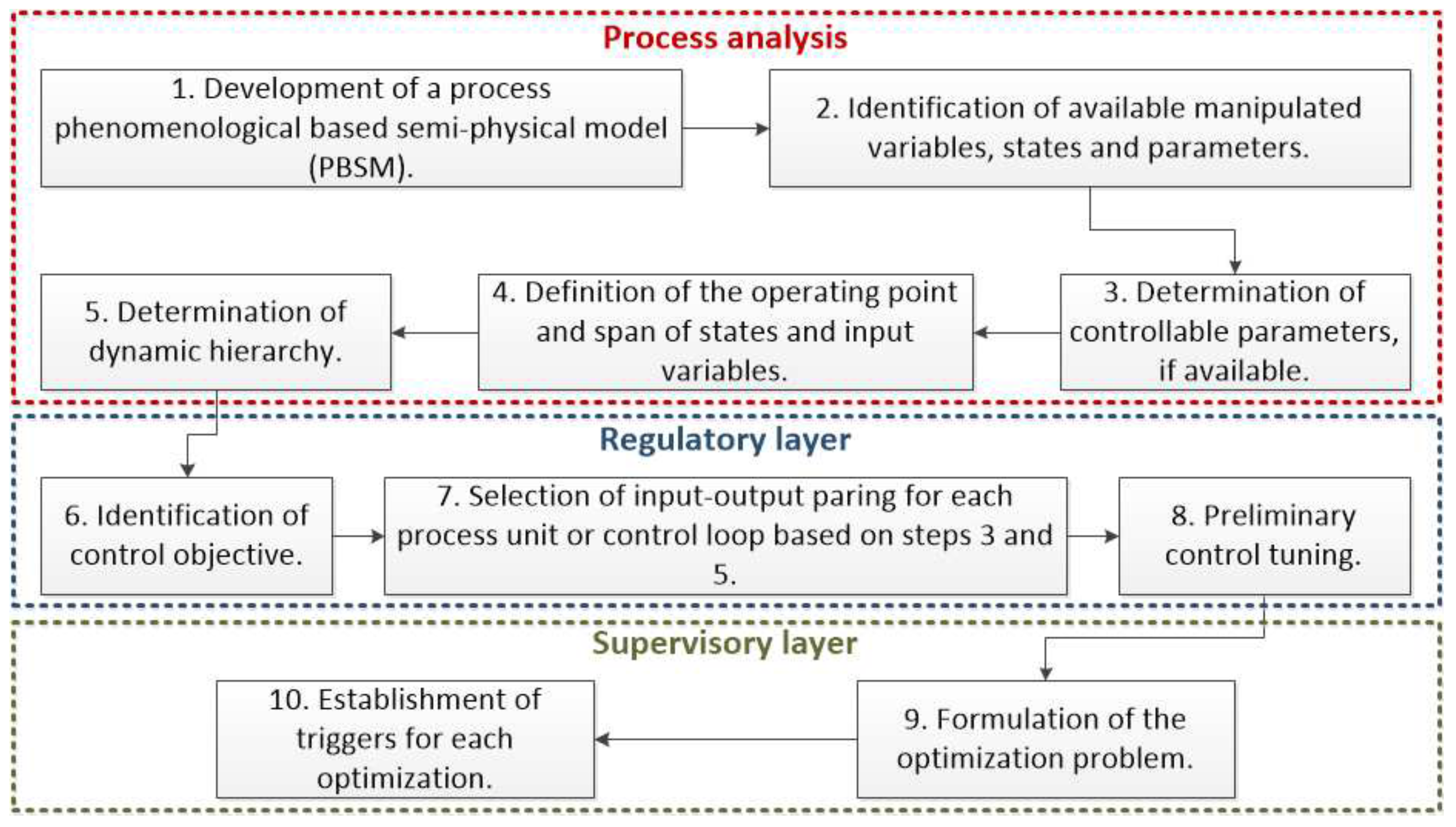
In the following, the methodology to develop a collaborative control proposed is described. In summary, collaborative control is a multivariable control strategy useful for processes with very different dynamic effects. All of the individual control loops work together, in spite of each one having different effects on the process and dynamic behavior. Figure 2 illustrates the proposed methodology.
The common practice in control is to take the process states as controlled variables, considering that all states can be measured. In this work, some process parameters, called controllable parameters, are additional controlled variables, which can be directly manipulated through available control actions. They give extra degrees of freedom to the process control adding more control loops. This option of control structure is particularly interesting where the process is strongly affected by the changes on some parameters, although sometimes this fact is not evident due to some process model simplifications.
The methodology proposal is formed by three stages. The first one is the process analysis, aiming to get a full knowledge of the process. This implies obtaining a mathematical description of the process, a model. The second stage consists of designing the regulatory control layer. This stage distributes PID control loops over the whole plant, following the decentralized control approach. These PID controllers act on tracking mode on secondary dynamics, or over controllable parameters. Only one PID in regulatory mode acts over the the main dynamic of the process. Finally, the third stage designs the supervisory control layer using an optimization problem formulated for including information regarding the main and the secondary dynamic, and the controllable parameters as an additional and new part. Following the procedure of [6], but including some modifications, each stage is explained in the next subsections.
2.1. Process Analysis
This obtains a phenomenological based semi-physical model for the treated process. Manipulated variables, states, and parameters are determined and a set of controllable parameters is established in accordance with a process dynamic response. Finally, the dynamic hierarchy is stated for the given process operation point.
Step 1: Obtaining a phenomenological based semi-physical model (PBSM) for the treated process. Developing a PBSM for the process is the first step for designing the proposed collaborative control structure. It should be noted that, if a PBSM is not available, the model can be obtained following the proposal presented in [23,24].
Step 2: Determinate available manipulated variables, states and parameters. For the treated process, the available manipulated variables u and the state variables x are stated from the mathematical model. During model simulation, it is possible to consider any variable or parameter as measured. However, in a real process, the available information depends on installed instruments or designed observers for these variables or parameters.
Step 3: Determinate the controllable parameters. If controllable parameters can be used in the process, this step determines the parameters to be considered as controllable ones. These parameters give the possibility of being controlled and fulfill the characteristics previously mentioned. That set of parameters are used to implement the collaborative control approach proposed here.
Step 4: Define the operating point and span of states and input variables. The real operation of the process is analyzed in this step. The stationary states of the process and its operation conditions are chosen. Such values will be used to determine the main dynamic reference value, the only fixed set point. In this step, the span of process states and input variables is defined in accordance with process operative conditions.
Step 5: Determine the dynamic hierarchy. This is the final step of process analysis, which results in being crucial for the collaborative control structure due to the result obtained defining the design of the supervisory layer. For this, the procedure proposed by [6,25] is used here. This procedure is based on singular value decomposition (SVD) of the Hankel matrix of the process, using the state impactability index ().
The Hankel matrix, H, is the input–output behavior of the process, establishing a relation between a sequence of past inputs and a sequence of future outputs of the process [6]. H is defined by the following Equation:
The SVD of Hankel matrix, showed in Equation (2), allows for calculating a measure for the dynamic effect of each process variable over process response and to determine the input—output pairings.
The state impactability index, presented in (3), is the impact of the manipulated inputs u of the process (taken as a whole) over the k-th process output variable :
where and are found using a SVD of the Hankel matrix H of the process model. p is defines as the number of non-negative singular values, n the number of state variables, the i-th singular value and and the orthonormalized eigenvectors and , respectively. In this way, is used to determine the main and secondary dynamics. Then, the main dynamic will be the state with higher . The rest of states will be the secondary dynamics.
In summary, the Hankel matrix is calculated in order to determine the dynamics hierarchy in the system and to select the dynamics for the supervisory layer. This procedure is performed offline, and no further results are obtained using calculations based on the Hankel matrix, which prevents obtaining unreliable results due to a large matrix condition number. In fact, the condition number is usually large, allowing for the division of dynamics between regulatory and supervisory layers.
2.2. Regulatory Layer Design
This task is dedicated to analyzing each one of the individual closed loops to be implemented on the plant. Such control loops include those controllers designed at the commissioning of the process to operate in regulatory mode, following the common practice in decentralized control strategy. Collaborative control strategy changes the secondary dynamic controllers from their regulatory mode to operate in tracking mode. These loops should track the set point given by the coordinator controller. In this level, the current proposal uses PID controllers due to this control strategy being easy to implement and understand.
Step 6: Identification of control objective. It consists of defining the control objective for the process as a whole and establishing the control objective of the pieces of equipment forming the process. The control objective is determined in accordance with hierarchical dynamics defined in Step 5 using Equation (3). In this sense, main dynamic is related directly with the main control objective of the process. It should be noted that it is possible to require additional control loops, which will be determined as it is declared in the following step.
Step 7: Selection of input–output pairing for control loop at each process unit, based on steps 3 to 5. In congruence with the control objectives of the process, this step states the control loops included in the regulatory layer. It is possible to use diverse strategies to determinate an adequate input–output pairings. For example, the RGA approach [26] or the SVD of the Hankel matrix as in [6].
Step 8: Preliminary control tuning. To finish the design of regulatory layer, the tuning of each proposed individual controller is executed here. For this task, any available tuning method for single-input/single-output (SISO) loops can be used, considering that any interaction among control loops should be considered on the supervisory layer. Nevertheless, these controllers should be individually evaluated regarding their performance, previously to design the supervisory layer.
2.3. Supervisory Layer Design
This step states an optimization problem considering the main and secondary dynamics, and the selected controllable parameters. The decision variables are the reference points for each one of the regulatory individual controllers. The values of such reference points look for reaching the global control objective through the minimization of main dynamic error, which is the only one variable with a control loop operating in regulatory mode.
Step 9: Formulation of the optimization problem. It is considered that the performance of regulatory level is good using fixed set points, but it is not enough regarding desired objectives of the plant wide control (PWC). The supervisory layer has a direct relation with the main dynamic and the stated optimization, with a direct collaboration of secondary dynamics and controllable parameters in order to fulfill the objectives of the plant as a whole. It should be noted that the effect of every secondary dynamic and controllable parameter over the main dynamic is exploited using the dynamics relations described in the process model. In this way, the set points of the control loops of secondary dynamics and controllable parameters are degrees of freedom in this optimization problem [6]. The optimization problem is formulated as:
where are the controlled variables and are the controlled parameters. , , and correspond to weights, which operates as tuning factors, represents the set point of the main dynamic () of the process, and is the value of at the steady-state that would be achieved if the process reached its steady-state over all the values determined by the optimization and the rest of states finished at the current value. corresponds to a sensitivity function of main dynamic regarding changes on i-th secondary dynamic at the current values of the process state, corresponds to the sensitivity function of main dynamic to changes on k-th controllable parameter at the current values of the process state. , , and represent limit values stated for the set points of secondary dynamics and controllable parameters, looking for guaranteeing the stability of the process. , , and indicate the maximum and minimum possible changes to apply in the references of secondary dynamics and controllable parameters.
| S. t. |
The term represents the effect of every secondary dynamic over the main dynamic and it is calculated using the Equation (5), with for the i-th secondary dynamic. Note that because one of the process dynamics is the main one:
In addition, the new sensitivity added to the cost function proposed in [27], which is related to the main dynamic and the controllable parameters, is formulated using the Equation (6).
It is noted that the stability of the plant as a whole is assumed as guaranteed provided all the local controllers are stable. Therefore, the design of these controllers should guarantee their stability, considering that the variations on their set point are limited by operation conditions, transport parameters, capabilities of the final control elements, and physical and chemistry properties, looking for guaranteeing that the control actions of local controller are into the stable region of the process plant considered as a whole. The superiority of the collaborative proposal consist on using PID as local controllers. In this way, a wide list of PID design techniques guaranteeing closed loop stability are available in published works.
Additionally, some characteristics of the objective function are: (i) The effect of disturbances is considered because the sensitivities and are computed at each sampling time; (ii) The sensitivities are algebraic expressions; for this reason, they are calculated with current measurements. In this sense, the measurements include the dynamic time evolution of the system, and a multi-step prediction as in Model Predictive Control is not necessary; and (iii) the process model is transformed considering explicit differentiation, while the process information is maintained [6].
Step 10: Establishment of triggers. This step determines some triggers for the optimization problems. When the main dynamic is near enough to its set point, the collaborative action is not required, being the main dynamic control loop which provides all control effort. Therefore, either the maximum set point deviation for the main dynamic, or the maximum cost value deviation in some number of past time steps, are useful as particular triggers [6].
3. Model Predictive Control (MPC)
In order to assess the results provided for the methodology proposed in this paper, an MPC has been considered in the supervisory layer, in particular, a centralized nonlinear MPC that provides the set points for the secondary layer, with the following objective function:
| S. t. | |
Here, and are the outputs and control variables, are the reference signals, , , are tuning matrices to guarantee stability and to weight the outputs and the control movements, respectively, is the control horizon, and are the initial and final prediction horizons, , , , , , and are bounds to be imposed on the system variables [28].
It should be noted that the MPC uses a receding horizon strategy with an internal prediction model. The control actions are calculated to minimise an index involving set point and predictions deviations in addition with the control movements over two horizons. In this work, the MPC scheme is based on the use of the following nonlinear discrete time prediction model:
where k is the current sampling point, and are the future control moves at time , with measurements up to time k.
4. BSM1 Process Description Including the Mass Transfer Model
The simulation benchmark used in this work is presented below together with some specific modeling of some process belonging to the aerobic section. In particular, phenomenological based semi-physical models, based on conservation principles, with constitutive and assessment equations for model parameters are used [23].
A plant for water treatment (WWTP) is formed by three main sections beginning with the primary treatment, which is included to reduce suspended solids and large pollutants, preparing wastewater for a secondary treatment. This last one comprises anoxic and aerobic zones. The last step is the tertiary treatment, for additional improvement of the effluent quality [29].
4.1. BSM1 Model
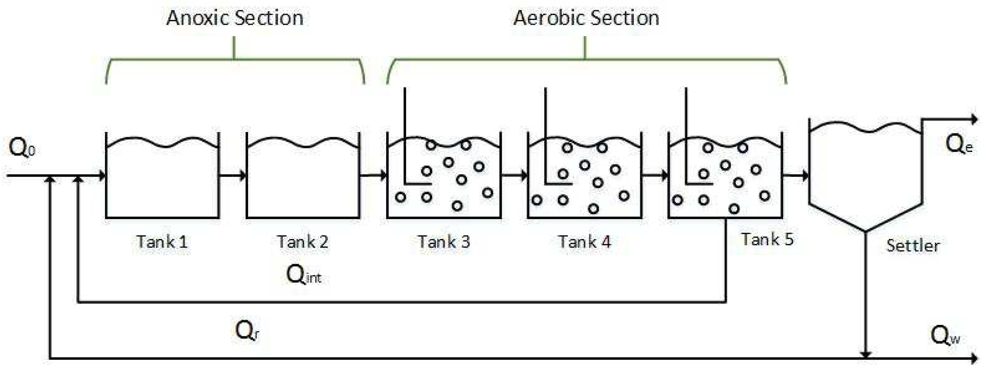
The BSM1 is a well known simulation benchmark for the biological process taking place in secondary treatment of WWTPs. It includes some influent sets for different weather conditions (dry, storm, and rain weather) and defines some performance indexes. The plant layout comprises two anoxic reactors where no dissolved oxygen is present (only bonded oxygen is possible), and three aerobic reactors (Figure 3). Finally, a secondary settler separate sludge from the clean water [30,31].
The aeration in the aerobic tanks are required for nitrification process and it is also relevant to determine the microorganisms metabolic route to degrade pollutants [31]. Therefore, the oxygen concentration is a key variable that must be maintained at a proper level. Note that that oxygen transfer rate depends mainly on reactor geometry, aerators arrangement, sludge characteristics, stir rate and air flow characteristics as a dispersed phase.
The BSM1 model has thirteen states: soluble and particulate inert organic matter (, ), readily and slowly biodegradable substrate (, ), active heterotrophic and autotrophic biomass (, ), particulate products from biomass decay (), dissolved oxygen (), nitrite and nitrate nitrogen (), plus nitrogen (), soluble and particulate biodegradable organic nitrogen (, ).
Then, mass balances are obtained for each state, forming the mathematical model presented below, where the subindexes represent the BSM1 state and the reactor number, respectively, w represents mass fractions, is mass rate in the flow k, V is the tank volume, and are the oxygen and the oxygen saturation concentration, respectively, is the reaction rate, and is total mass for component i:
- Mass balance for reactor number one:
- From the second anoxic reactor to the fifth reactor (second reactor as an example):
- Special case for oxygen (fifth reactor as an example):
The main constitutive equations for this mathematical model are all the reaction rates and the mass transfer equation. The reaction rates are conformed by biological processes and other parameters, and the details are given in [31]. The accuracy of the BSM1 model considered as a case study to apply the methodology proposed is based on the wide use of this benchmark in the literature in the last decade, and its recognition by practitioners in the wastewater treatment field. There are a large amount of research work supporting its validity, and there are also some extensions, such as BSM2, enlarging the activated sludge process with the primary and sludge treatment in a WWTP. Moreover, this benchmark is based on the well known ASM1 model (Activated Sludge Model No 1), developed by [30].
It is important to describe the operational objectives of BSM1, which are considered to evaluate the performance of the methodology proposed [31]. Particularly, in this work, pumping energy (PE), aeration energy (AE), and effluent quality (EQ) are evaluated. Additionally, ISE (Integral of Squared Error) and IAE (Integral of Absolute Error) are considered:
where is the period of observation, is the initial time, and are the internal and purge recycling flows, is the oxygen saturation concentration, is the volume of reactor k, is the volumetric oxygen mass transfer coefficient, are weighting factors for the different types of pollutants, represents the suspended solids, is the effluent chemical oxygen demand, is the Kjeldahl nitrogen concentration, is nitrite and nitrate concentration, is the biological oxygen demand, and is the effluent flow.
4.2. Mass Transfer Model
The mass transfer coefficient represents a constitutive equation of the model, although this coefficient is not modeled in detail in BSM1. There it is only represented by a volumetric oxygen mass transfer coefficient (), and it is calculated only with dependence on the temperature and some other empirical parameters. Particularly, it is represented by Equation (17):
where T is temperature in the system and , F and are some empirical parameters. Obviously, this expression for does not represent faithfully the real process because it does not describe other physical phenomena with a paramount influence on the mass transference, such as the size of bubbles and the gas hold up [32,33]. Moreover, in real practice, it is not possible to manipulate the because it does not represent a physical handle. In fact, is the product between the liquid phase mass transfer coefficient () and the specific interfacial area (a). In order to understand the gas—liquid mass transfer procedure, it is necessary to separate these parameters because they are differently affected by manipulated variables. In this work, an improved model for has been developed and it is presented below.
The bubble formation is an equilibrium between gas pressure (expanding the bubble) and superficial tension (aiming to burst the bubble). This formation takes place in two steps [34], the expansion step and the detachment step. Note that the equilibrium not only depends on the physico-chemical properties of the materials, but also on the energy applied to stir the fluid [35]. The bubble formation is relevant because the size and quantity of bubbles define the oxygen transfer in the aerobic reactors. Bubble diameter, is obtained by (18) [36], where is the orifice diameter of the diffuser membrane (m), is the surface tension (), is the difference of the liquid and gas densities (kg/m), and g is the gravity:
is calculated according to:
where is the liquid density, considered here as pure water density, and the gas density, obtained using the ideal gas equation with the internal pressure of the bubble :
with the molecular weight of the gas, R the Ritcher constant, and is the gas temperature. The bubble internal pressure () is calculated in (21) with the gas injection pressure and the gas drop pressure in the diffuser orifice:
where is the injection pressure and the drop pressure in the diffuser orifice [37]:
with the gas flow rate through the orifice and the orifice constant (). This constant is a function of gas flow rate, density (), and viscosity (), orifice plate thickness (L), and orifice diameter (). It is evaluated with the following expression:
where is a dimensionless constant:
with the Fanning friction factor. For laminar flow, this factor is obtained as:
where is the Reynold number.
Then, the mass transfer coefficient is obtained considering the liquid-phase mass transfer coefficient and the gas-liquid interfacial area a separately. As this coefficient quantifies the velocity of species movement across an interphase [38], it is useful to estimate the mass transfer rate. The dependence on the presence of pollutants is very high [38,39]. Moreover, considers the effects of the liquid movement around the gas bubbles and the specific area a reflects the behavior of the bubbles [40]. In [32,41], some empirical correlations to obtain are given. In this case, Kawase correlation has been selected because it has been applied in similar conditions to BSM1, and it complies with the required operation range for BSM1 [32]:
where is the gas diffusivity in liquid (m/s), the liquid viscosity ( /cdot s), the superficial gas velocity (m/s) and g the gravity constant (m/s). The superficial gas velocity is obtained as volumetric flow rate () passing through the active cross sectional area of the diffuser. In turn, this area represents the empty spaces of diffuser, calculated from the membrane porosity. The diffusers chosen in this work are membrane type (wastewater treatment plant El Marin in Salamanca, Spain), due to its high available active area (). Then, the superficial gas velocity is:
As for the specific area (a), it can be obtained as the interfacial area (gas-fluid) per unit of volume [42]. Then, a is obtained according to (28) given by [43], where the bubbles are considered as spheres [44]:
where is the gas hold-up and is the bubble diameter. The gas hold-up can be seen as the gas retention in the fluid. More precisely, is affected by the diameter of the diffuser orifice, liquid density, superficial gas velocity, and surface tension [45]. There are many empirical expressions to obtain because it affects the mass transfer directly [46]. One of them is [32], where different systems and fluids have been considered. Here, the physical conditions are similar because a column was considered to represent a vertical slide of an activated sludge reactor. However, according to the operating conditions and the of mass transfer taken place, the following equation is chosen:
5. Application of the Methodology to BSM1
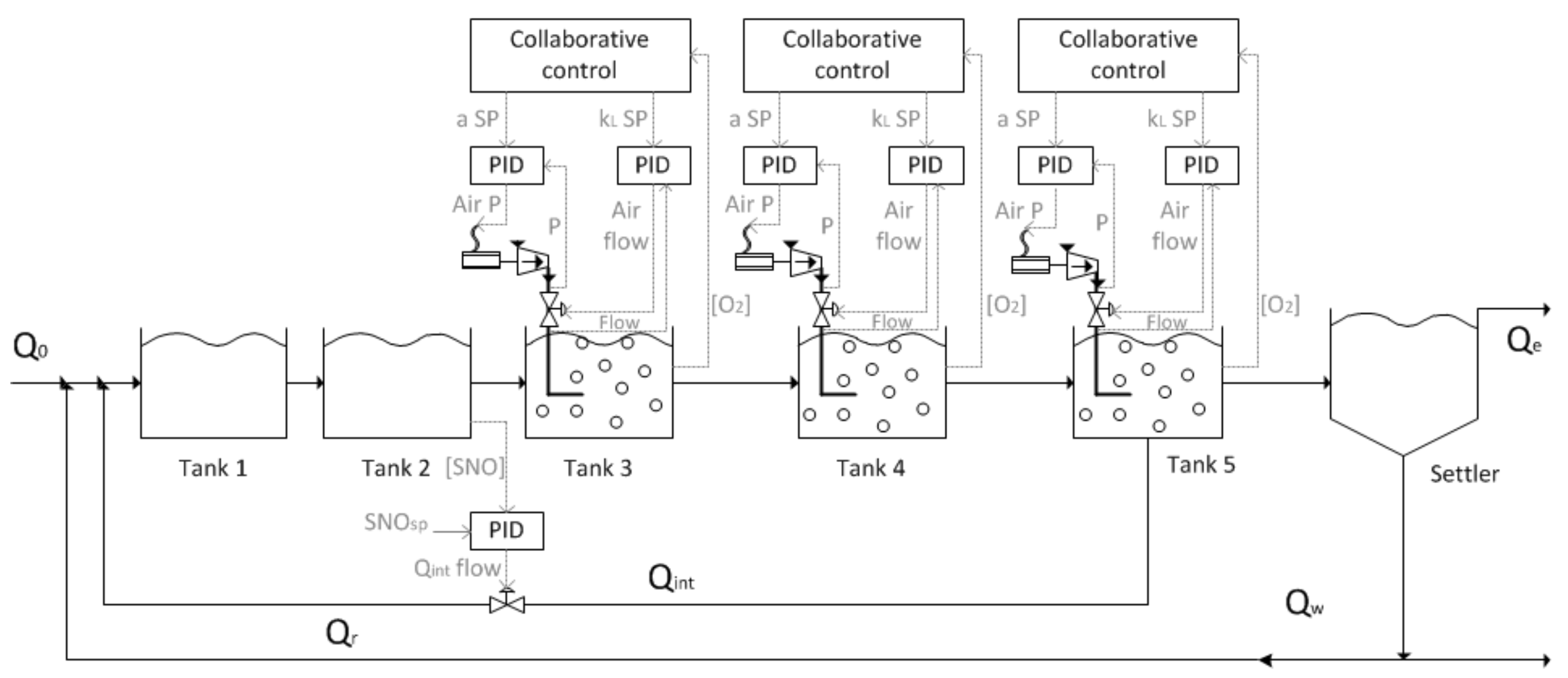
The collaborative control strategy previously described is applied to BSM1 oxygen control in this section. Note that, for the oxygen mass transfer, separated expressions for and a are considered.
Step 1.Development of a PBSM. The wastewater treatment plant is simulated in accordance with BSM1 model equations where a high variability of the influent dynamic characteristics (flow and concentration variables) is implemented [31]. It should be highlighted that proposed collaborative control approach is focused on the aerobic section, for this reason, the mass transfer model presented previously is required.
Step 2.Manipulated variables, states and parameters. According to BSM1, the states considered are thirteen, corresponding to the compounds studied in BSM1. Moreover, there exist many parameters in this process: kinetic and stoichiometric parameters, physicochemical properties as density and viscosity, temperature, design parameters as volume, diffuser specifications, and finally and a. The manipulated variables are related with recirculation flows ( and ), inlet flow (), air flow () and air injection pressure ().
Step 3.Selection of Controllable parameters. In BSM1, among other existing parameters, and a in the aerobic reactors are controllable ones because they are process parameters that can be directly manipulated using a control action. In this sense, and a can be controlled by air flow () and air injection pressure () in each reactor, respectively.
Step 4.Operation conditions and range of variation of states and inputs. The operation conditions are fixed by BSM1 conditions. In this way, the set point for oxygen concentration and total nitrogen concentration are taken form [31]. In this sense, in the second anoxic reactor, the reference for the nitrite+nitrate concentration is stated in 1 g/m. The oxygen concentration in aerobic section is 1.63, 2.47 and 2 g/m in the third, fourth and fifth reactor, respectively.
Step 5.Dynamic hierarchy. The design of the collaborative control structure requires the definition of the dynamic hierarchy. This is determined in accordance with the state impactability index . The state () presenting the highest defines the main dynamic while the rest of the states are the secondary ones. The values are shown in Table 1. According to the values presented in the table, the process main dynamic is the oxygen concentration being the secondary ones defined by the other variables considered in the table.
Step 6.Control objective. The oxygen concentration is the main dynamic in each reactor; consequently, the collaborative control objective is to regulate the oxygen concentration on a prescribed value defined by the set point. For this reason, the oxygen concentration is regulated using the collaborative control strategy while nitrite + nitrate concentration is controlled by means of an independent PID controller. In addition, other process goal is to fulfill the environmental regulations by keeping the total nitrogen, COD, TSS, and oxygen concentrations below some well established legal limits.
Step 7.Input–output pairing. The control methodology is implemented in the three aerated reactors. In this sense, the system has two controllable parameters in each reactor, and a. The main goal of the coordinator control implemented in the supervisory level is to control the oxygen concentration, this being a fixed objective. Moreover, a pair of simple controllers, in the lower level, cooperate to fulfill this goal. These two simple control loops are related to the parameters and a. The first ones changes the air flow and the second the pressure of the injected air to control and a, respectively (see Figure 4). As mentioned before, to keep nitrite and nitrate concentration at a prescribed value given by the set point, an independent PID controller is used, where the manipulated variable is the internal recycling flow.
Step 8.Preliminary control tuning. The preliminary control tuning is focused in a regulatory layer. PIDs controllers are tuning using the values given by the Ziegler–Nichols method as seeds, but with a further fine manual tuning. The PIDs controllers are implemented using:
being the manipulated variable at time , the proportional gain, the difference between set point and process output variable at time . is the integral time, the derivative time, and is the sampling time. Table 2 presents the corresponding values for the current application.
Step 9.Optimization problem. Supervisory layer is based on one optimization problem. In this sense, Equation (4) is implemented taking into account the dynamic hierarchy established in step 5. The optimization problem is reduced to Equation (31). In this case, only controllable parameters are in the objective function and secondary dynamics are not taken into account because they do not have available manipulate variables in order to achieve the control objective:
| s. t. |
The tuning parameters used are , and , with values 1, 1 and 0.1, respectively. It is important to highlight that is the stationary value of oxygen concentration variable when the lower layer control loops maintain the and a at the values evaluated by solving the optimization problem previously stated, keeping the rest of process states at their current values. By solving the optimization problem defined above, the set points for and a are evaluated and the PIDs manipulate the corresponding control variables to respond to set point changes. Note that and are calculated by means of Equations (32) and (33). These expressions were obtained from the process model (BSM1) as follows:
Step 10.Triggers of optimization. In this case, deviations greater than 5% on the main dynamic ( concentration) were defined as optimization triggers.
6. Results and Discussion
In this section, some results of collaborative control applied to BSM1 are presented and compared with the use of an MPC strategy in the supervisory layer. The controller structure for collaborative control is shown in Figure 4. In the case of the MPC controller, the controlled variables are the oxygen concentration in the fifth reactor and the nitrate+nitrite concentration in the second reactor, while the set points of , and the internal recycling flow are the manipulated variables. Then, the MPC controller structure is analogous to the collaborative control one, except for the case of dissolved oxygen in reactors 3 and 4, which have been removed from the MPC structure by simplicity. Note that, in both strategies, there are PID local controllers for regulation in the lower layer, with , and as manipulated variables. For all simulations, the dry weather influent of BSM1 has been considered, having a daily peak of flow and pollutants that is somehow reflected in all concentrations throughout the plant. The simulation time is eight days.
Regarding the MPC tuning, although there are many tuning methodologies available, in this paper, the focus is on the new collaborative control strategy developed, and therefore the MPC tuning has been performed systematically only by trial and error. As for PID tuning, the Ziegler–Nichols method has been applied, with a further fine-tuning to prevent aggressive behavior. This is the current industry practice, taking Ziegler–Nichols settings as seed parameters but applying a trial and error procedure to obtain the final tuning.
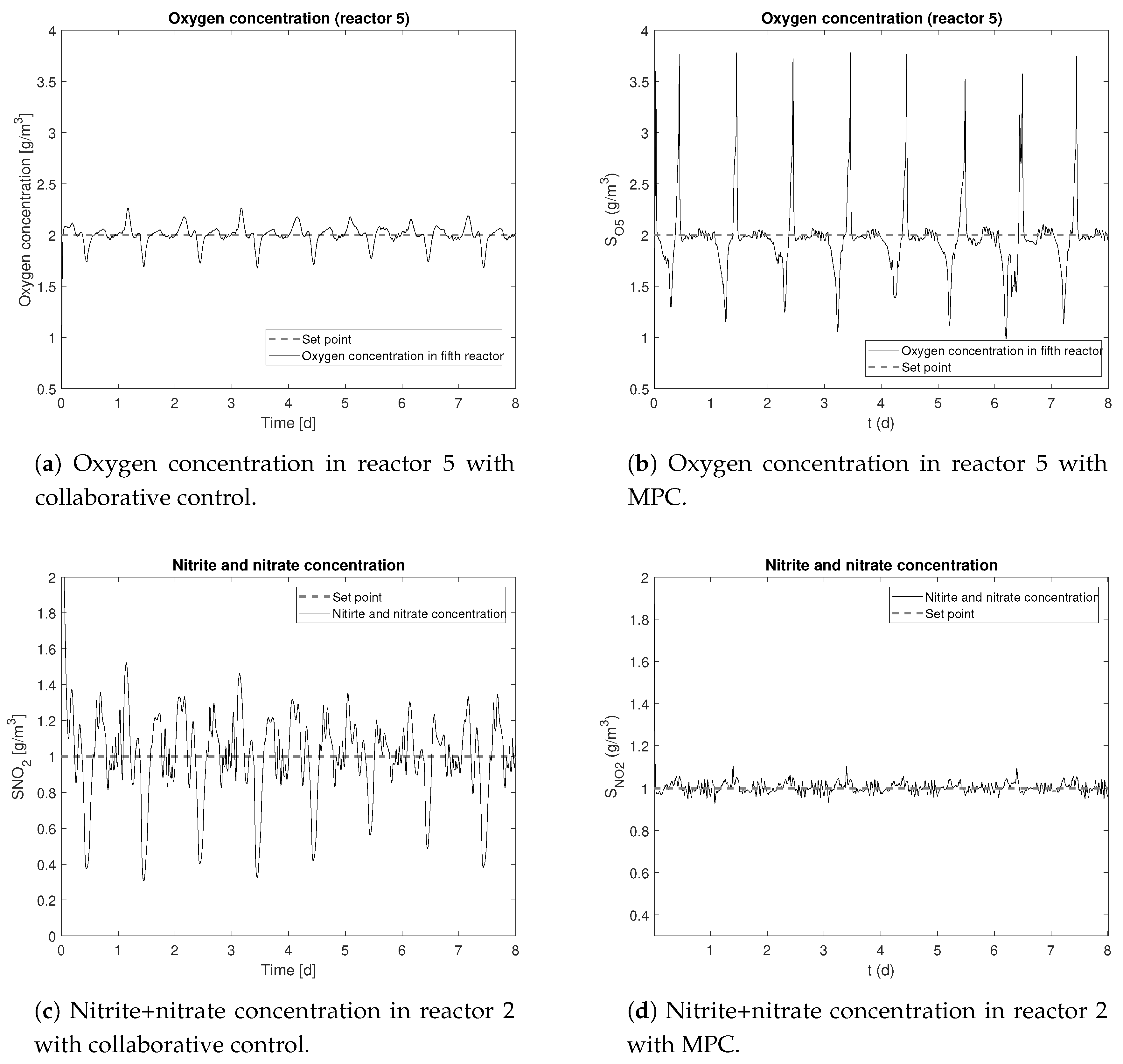
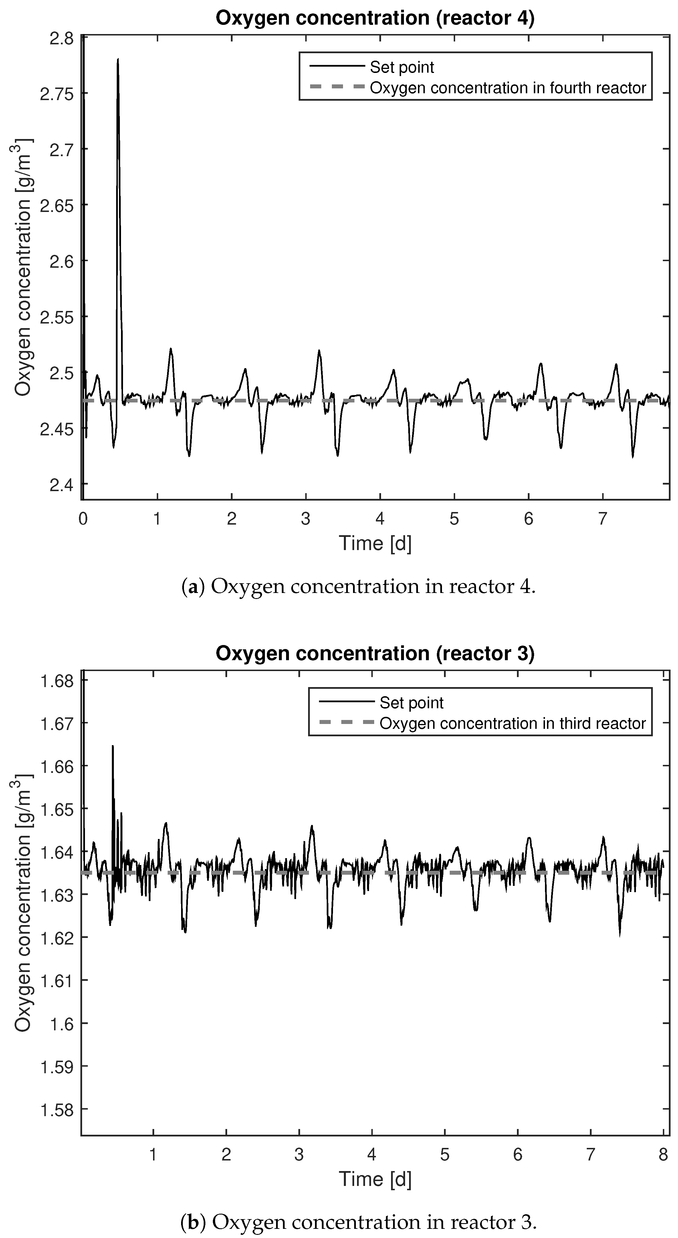
In Figure 5, the dynamic evolution of the controlled variables for both strategies is presented, specifically the oxygen concentration in the fifth reactor and the nitrite+nitrate concentration in the second reactor, showing good set point tracking with some periodic oscillations due to the daily high variability of the plant influent. Although MPC presents better tracking for nitrite+nitrate concentration, collaborative control presents better behavior for oxygen concentration because this is the main dynamics in this strategy. Moreover, in collaborative control, the PID for nitrite+nitrate concentration is independent of the collaborative loops. In Figure 6, the oxygen concentration in the third and fourth reactors using collaborative control is presented, also with good tracking.
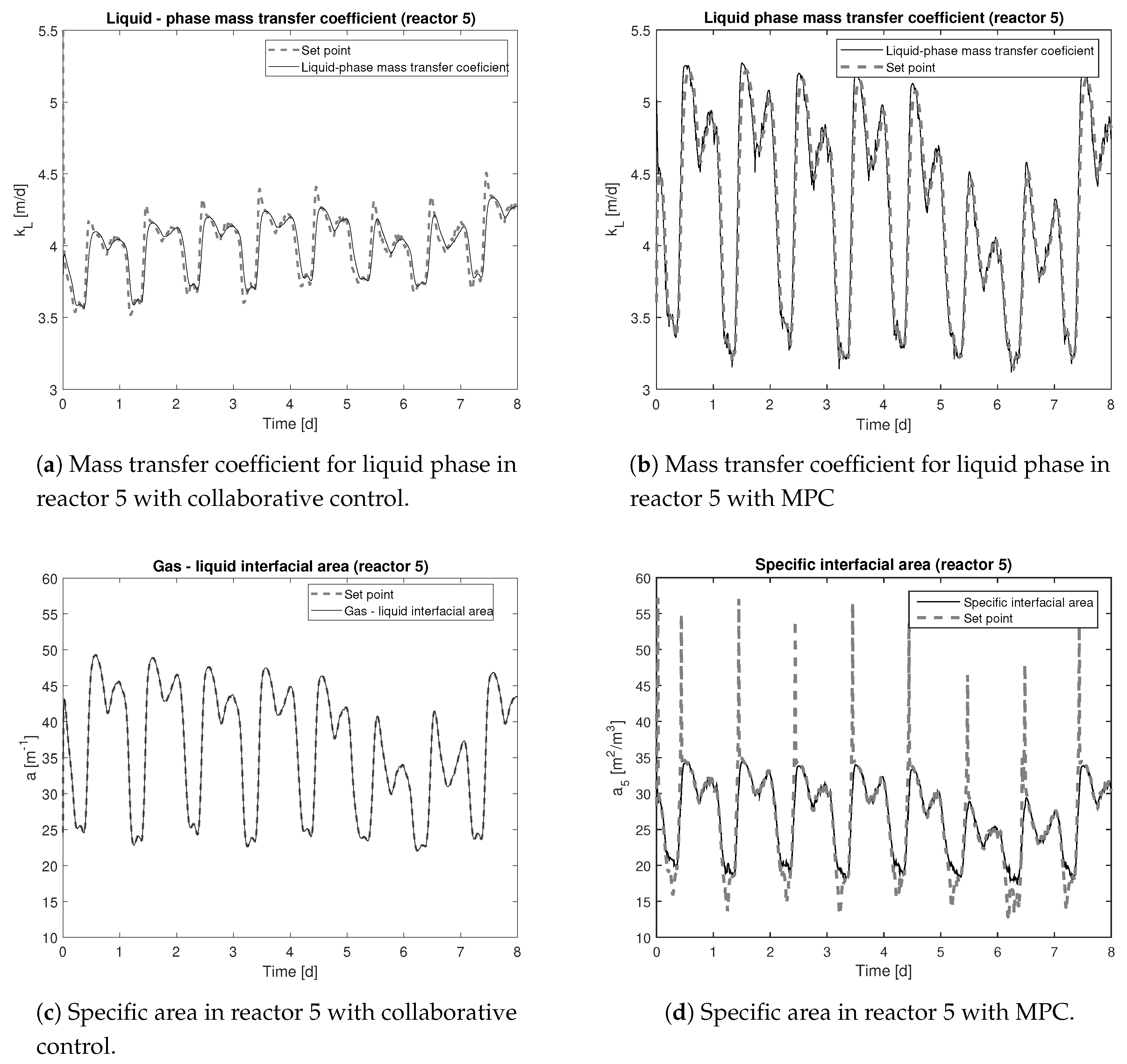
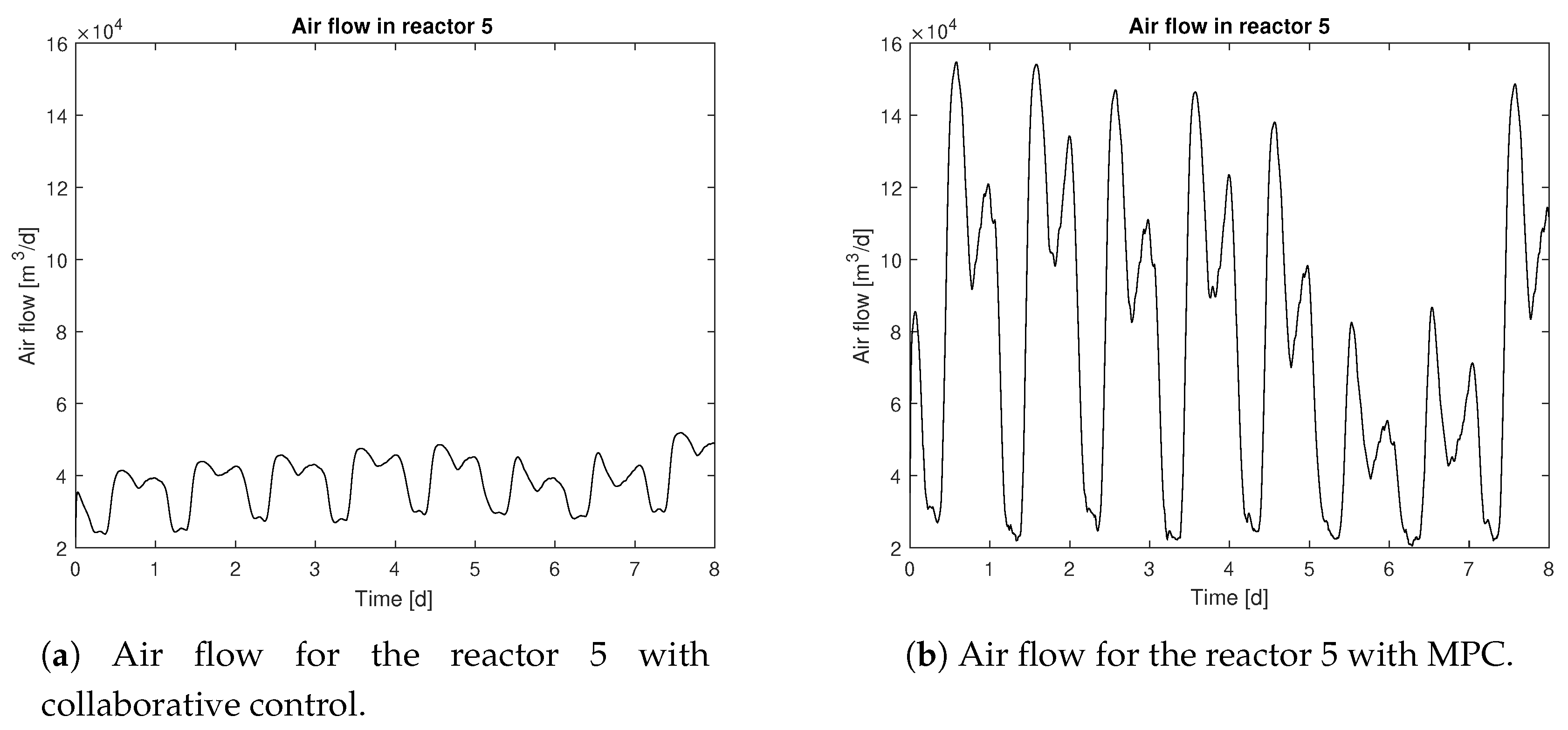
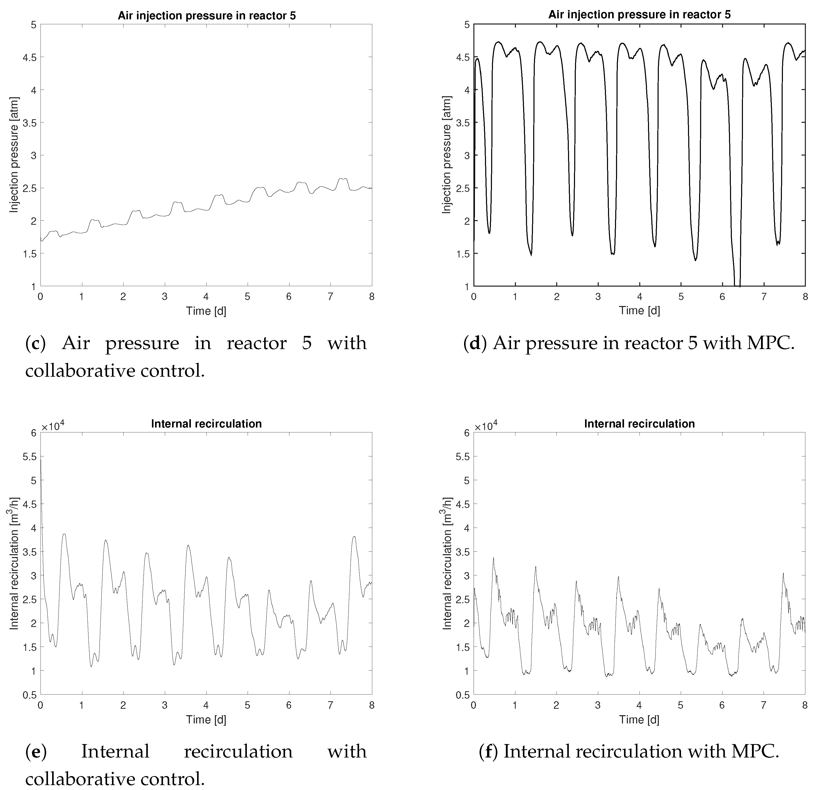
The set point tracking of controllable parameters (Figure 7) is also good, following the references given by the supervisory layer. Additionally, in Figure 8, the control actions , are presented. Note that the set points provided by the MPC are more aggressive than those provided by the collaborative control, due to a more frequent update performed by the MPC optimization problem, while in collaborative control only the optimization triggers command the set point change by solving Equation (31). Finally, the internal recirculation flow is similar for both strategies, due to the relative independence of control loop in the second reactor for collaborative control strategy.
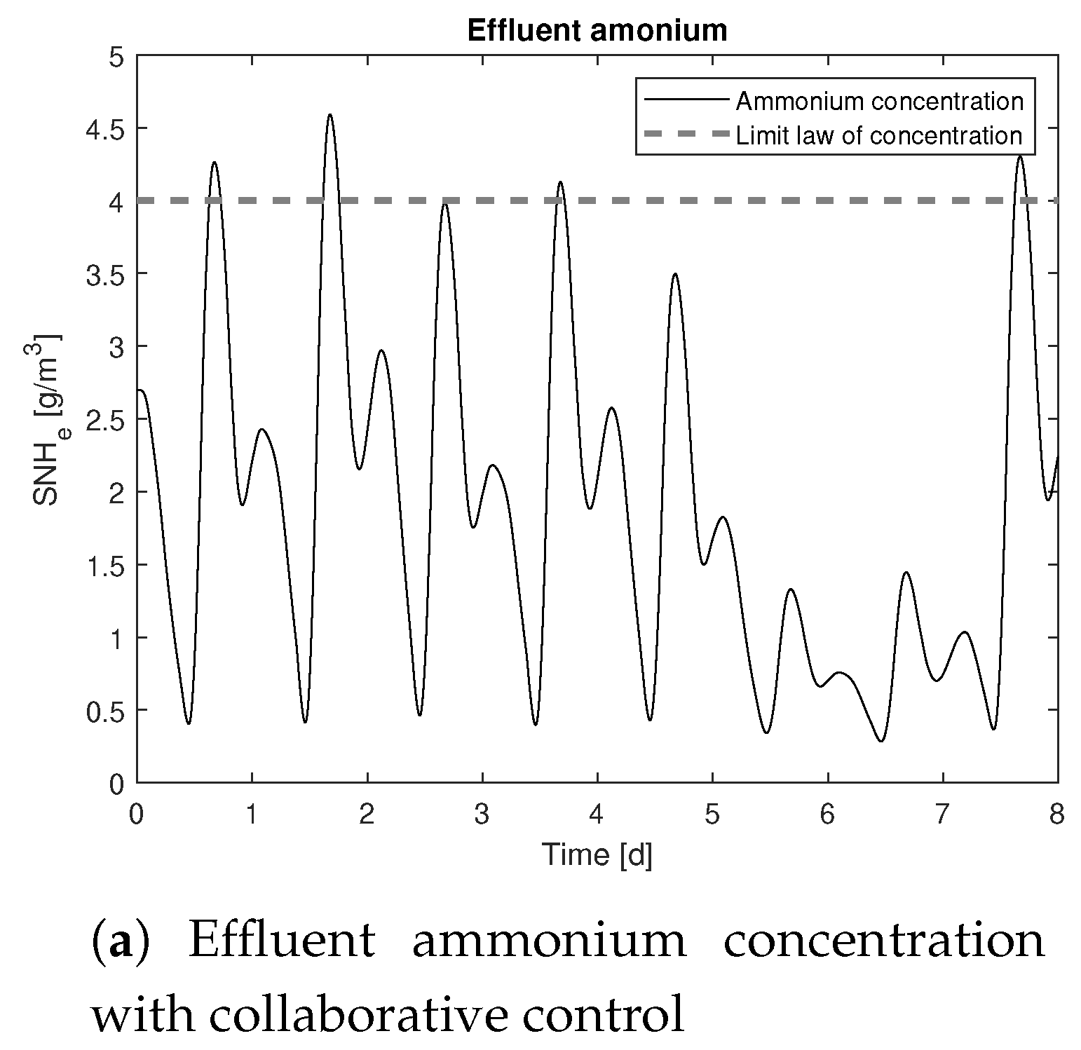
In Figure 9, the ammonium in the effluent is presented, where, in the case of collaborative control, some violations of the legal limit of 4 mg/L can be seen, but only in very short periods of time. On the other hand, for the MPC, there are no violations of the limit, but at the expense of larger variations in the oxygen concentration (Figure 5b) required in the biological processes to decrease the effluent ammonium concentration.
For a better comparison of the proposed methodologies, Table 3 presents the following performance indexes: ISE and IAE for oxygen set point tracking, energy for pumping (PE), energy for aeration (AE), and the quality of the effluent (EQ). Moreover, these indexes are compared with [18], where an economic oriented MPC controller and a default PI strategy without supervisory layer [31] is implemented, in order to evaluate the general performance of the methodology proposed in our work. From these indices, it can be seen that collaborative control strategy presents better ISE and IAE than MPC controller for oxygen control, as can also be seen in figures with the dynamic evolution of this concentration. On the other hand, PE and AE are better in MPC due to smaller control actions required by the supervisory layer in this case. Finally, EQ is shown here as an additional index for performance, though it has not been included directly in the methodology. Although the EQ value for collaborative control is a bit higher than for the MPC structure, it is still acceptable, particularly if it is compared to [18].
7. Conclusions
This paper proposes a novel collaborative control structure taking into account in its design the plant dynamical characteristics, establishing a dynamic hierarchy by using the Hankel matrix of the process model and the control of specific parameters by means of simple PID control loops, which is especially attractive for industrial applications. The methodology proposed has been tested in the control of a specific process of wastewater treatment plant, particularly using the BSM1 benchmark.
The good results obtained for set point tracking show the efficiency of the proposed methodology, when it is compared to other structures reported in the literature such as the ones based on MPC. The method complexity and the computational load reductions are some of the most remarkable characteristics, in comparison with MPC, which makes the presented proposal very suitable to be applied to large-scale processes. This computational reduction is mainly due to the fact that the calculation of inputs and states predictions over some time horizon is not further needed. In the proposed methodology, the decision variables are evaluated without solving the complete model at each sampling time.
Although it might be possible to achieve better performance with the MPC due to higher complexity of the optimization problem, the results obtained should be evaluated considering the difficulties with MPC tuning. In fact, one of the main advantages of the collaborative control strategy is the simplicity, including an easier tuning because only weights and must be selected. Note also the particular difficulties in considering BSM1 process as a case study due to remarkable different dynamics (nitrogen, oxygen) and disturbances. Moreover, the inclusion of the nitrate+nitrite concentration as a controlled variable within the multivariable MPC framework further increases its complexity and therefore its performance is worsened.
The collaborative control outperforms the conventional MPC/PID control structure depending obviously on the process considered because both methodologies have their advantages and drawbacks. Anyway, a general criterion to apply the collaborative control is that it may be valuable for industrial complex processes with difficult dynamics, where the use of other prediction-based controllers (such as MPC) need a time-consuming tuning and an optimization routine executed each sampling time.
Finally, it is important to mention that the use of a detailed model for the mass transference is also a novelty of the work. The advantage compared to other simpler models is the improved description of the real phenomenon making the choice of controllable parameters easier. In addition to this, it represents the relationship between controllable parameters and manipulated variables in a straightforward way, increasing the degrees of freedom to control the process. The validation of this mass transfer has been performed in comparison with the model proposed in [31], with adequate results.
Author Contributions
K.M.-R., M.F., and H.A. conceived and designed the general approach; K.M.-R. and H.A. performed the simulations; M.F. and H.A. contributed to the simulation interpretations; writing—review and editing, M.F., H.A., and S.R.; supervision, P.V.; K.M.-R., M.F. and H.A. wrote the paper. All authors have read and agreed to the published version of the manuscript.
Funding
This work has received financial support from the Spanish Government through the MICINN project PID2019-105434RB-C31 and the Samuel Solórzano Foundation through project FS/20-2019.
Conflicts of Interest
The authors declare no conflict of interest.
References
- Kariwala, G.P.R.V. Plantwide Control: Recent Developments and Applications; John Wiley & Sons: Hoboken, NJ, USA, 2012; p. 494. [Google Scholar]
- Zumoffen, D.A.R. Oversizing analysis in plant-wide control design for industrial processes. Comput. Chem. Eng. 2013, 59, 145–155. [Google Scholar] [CrossRef] [Green Version]
- Shaoyuan, L.; Zheng, Y. Distributed Model Predictive Control for Plant-Wide Systems, 1st ed.; John Wiley & Sons: Hoboken, NJ, USA, 2016; pp. 1–13. [Google Scholar]
- Scattolini, R. Architectures for distributed and hierarchical Model Predictive Control—A review. J. Process Control 2009, 19, 723–731. [Google Scholar] [CrossRef]
- Skogestad, S. Control structure design for complete chemical plants. Comput. Chem. Eng. 2004, 28, 219–234. [Google Scholar] [CrossRef]
- Moscoso-Vasquez, H.M.; Monsalve-Bravo, G.M.; Alvarez, H. Model-based supervisory control structure for plantwide control of a reactor-separator-recycle plant. Ind. Eng. Chem. Res. 2014, 53, 20177–20190. [Google Scholar] [CrossRef]
- Maciejowski, J.M. Predictive Control: With Constraints; Prentice Hall: Upper New Jersey River, NY, USA, 2002. [Google Scholar]
- Qin, S.J.; Badgwell, T.A. A survey of industrial model predictive control technology. Control Eng. Pract. 2003, 11, 733–764. [Google Scholar] [CrossRef]
- Devadasan, P.; Zhong, H.; Nof, S.Y. Expert systems with applications Collaborative intelligence in knowledge based service planning. Expert Syst. Appl. 2013, 40, 6778–6787. [Google Scholar] [CrossRef]
- Carlson, T.; Demiris, Y.; Member, S. Collaborative control for a robotic wheelchair: Evaluation of performance, Attention, and Workload. IEEE Trans. Syst. Man Cybern. Part B 2011, 42, 876–888. [Google Scholar] [CrossRef] [Green Version]
- Fong, T.; Grange, S.; Thorpe, C.; Baur, C. Multi-robot remote driving with collaborative control. In Proceedings of the 10th IEEE International Workshop on Robot and Human Interactive Communication, Paris, France, 18–21 September 2001; pp. 237–242. [Google Scholar] [CrossRef] [Green Version]
- Ochoa, S.; Wozny, G.; Repke, J.U. Plantwide optimizing control of a continuous bioethanol production process. J. Process. Control 2010, 20, 983–998. [Google Scholar] [CrossRef] [Green Version]
- Marquez, A.; Gomez, C.; Deossa, P.; Espinosa, J.J. Hierarchical control of large scale systems: A zone control approach. In Proceedings of the 13th IFAC Symposium on Large Scale Complex Systems: Theory and Applications, Shanghai, China, 7–10 July 2013; Volume 13, pp. 438–443. [Google Scholar]
- Dang, P.; Banjerdpongchai, D. Design of integrated real-time optimization and model predictive control for distillation column. In Proceedings of the 2011 8th Asian Control Conference (ASCC), Kaohsiung, Taiwan, 15–18 May 2011; Volume 1, pp. 988–993. [Google Scholar]
- Marti, R.; Sarabia, D.; Navia, D.; De Prada, C. Coordination of distributed model predictive controllers using price-driven coordination and sensitivity analysis. In Proceedings of the 10th IFAC International Symposium on Dynamics and Control of Process Systems, Mumbai, India, 18–20 December 2013; Volume 10, pp. 215–220. [Google Scholar] [CrossRef] [Green Version]
- Scheu, H.; Marquardt, W. Sensitivity-based coordination in distributed model predictive control. J. Process Control 2011, 21, 715–728. [Google Scholar] [CrossRef]
- Kadam, J.V.; Marquardt, W. Sensitivity-Based Solution Updates in Closed-Loop Dynamic Optimization. In Proceedings of the 7th IFAC Symposium on Dynamics and Control of Process Systems 2004 (DYCOPS -7), Cambridge, CA, USA, 5–7 July 2004; Volume 37, pp. 947–952. [Google Scholar] [CrossRef]
- Revollar, S.; Vega, P.; Vilanova, R.; Francisco, M. Optimal Control of Wastewater Treatment Plants Using Economic-Oriented Model Predictive Dynamic Strategies. Appl. Sci. 2017, 7, 813. [Google Scholar] [CrossRef]
- Zhang, A.; Yin, X.; Liu, S.; Zeng, J.; Liu, J. Chemical Engineering Research and Design Distributed economic model predictive control of wastewater treatment plants. Chem. Eng. Res. Des. 2018, 141, 144–155. [Google Scholar] [CrossRef]
- Holenda, B.; Domokos, E.; Rédey, Á.; Fazakas, J. Dissolved oxygen control of the activated sludge wastewater treatment process using model predictive control. Comput. Chem. Eng. 2008, 32, 1270–1278. [Google Scholar] [CrossRef]
- Rojas, J.D.; Flores-Alsina, X.; Jeppsson, U.; Vilanova, R. Application of multivariate virtual reference feedback tuning for wastewater treatment plant control. Control Eng. Pract. 2012, 20, 499–510. [Google Scholar] [CrossRef]
- Vega, P.; Revollar, S.; Francisco, M.; Martín, J.M. Integration of set point optimization techniques into nonlinear MPC for improving the operation of WWTPs. Comput. Chem. Eng. 2014, 68, 78–95. [Google Scholar] [CrossRef]
- Hoyos, E.; López, D.; Alvarez, H. A phenomenologically based material flow model for friction stir welding. Mater. Des. 2016, 111, 321–330. [Google Scholar] [CrossRef]
- Lema-Perez, L.; Muñoz-Tamayo, R.; Garcia-Tirado, J.; Alvarez, H. Informatics in Medicine Unlocked on parameter interpretability of phenomenological-based semiphysical models in biology. Inform. Med. Unlocked 2019, 15, 100158. [Google Scholar] [CrossRef]
- Monsalve-Bravo, G.M.; Moscoso-vasquez, H.M.; Alvarez, H. Scaleup of Batch Reactors Using Phenomenological-Based Models. Ind. Eng. Chem. Res. 2014, 53, 9439–9453. [Google Scholar] [CrossRef]
- Arkun, Y.; Downs, J. A general method to calculate input–output gains and the relative gain array for integrating processes. Comput. Chem. Eng. 1990, 14, 1101–1110. [Google Scholar] [CrossRef]
- Moscoso-Vásquez, H.M. A Design Procedure for a Supervisory Control Structure in Plantwide Control. Master’s Thesis, Universidad Nacional de Colombia, Bogotá, Colombia, 2013. [Google Scholar]
- Francisco, M.; Skogestad, S.; Vega, P. Model predictive control for the self-optimized operation in wastewater treatment plants: Analysis of dynamic issues. Comput. Chem. Eng. 2015, 82, 259–272. [Google Scholar] [CrossRef] [Green Version]
- Ramalho, R.S. Tratamiento de Aguas Residuales; Editorial Reverté: Barcelona, Spain, 1996. [Google Scholar]
- Henze, M.; Gujer, W.; Mino, T.; Van Loosdrecht, M. Activated Sludge Models ASM1, ASM2, ASM2d and ASM3; IWA Publishing: London, UK, 2000; pp. 5–37. [Google Scholar]
- Alex, J.; Benedetti, L.; Copp, J.; Gernaey, K.V.; Jeppsson, U.; Nopens, I.; Pons, M.; Rieger, L.; Rosen, C.; Steyer, J.P.; et al. Benchmark simulation model no. 1 (BSM1). Ind. Electr. Eng. Autom. 2008, TEIE-7229, 1–62. [Google Scholar]
- Dudle, J. Mass transfer in bubble columns: A comparasion os correlations. Water Res. 1995, 29, 1129–1138. [Google Scholar] [CrossRef]
- Bouaifi, M.; Hebrard, G.; Bastoul, D.; Roustan, M. A comparative study of gas hold-up, bubble size, interfacial area and mass transfer coefficients in stirred gas-liquid reactors and bubble columns. Chem. Eng. Process. Process. Intensif. 2001, 40, 97–111. [Google Scholar] [CrossRef]
- Ramakrishnan, S.; Kumar, R.; Kuloor, N. Studies in bubble formation—I bubble formation under constant flow conditions. Chem. Eng. Sci. 1969, 24, 731–747. [Google Scholar] [CrossRef]
- Müller-Fischer, N.; Suppiger, D.; Windhab, E.J. Impact of static pressure and volumetric energy input on the microstructure of food foam whipped in a rotor-stator device. J. Food Eng. 2007, 80, 306–316. [Google Scholar] [CrossRef]
- Prieve, D. Unit Operation of Chemical Engineering; Carnegie Mellon University Press: Pittsbugh, PA, USA, 2000; pp. 199–247. [Google Scholar]
- Yang, G.Q.; Luo, X.; Lau, R.; Fan, L.S. Bubble formation in high-pressure liquid—Solid suspensions with plenum pressure fluctuation. AIChE J. 2000, 46, 2162–2174. [Google Scholar] [CrossRef]
- Olsen, J.E.; Dunnebier, D.; Davies, E.; Skjetne, P.; Morud, J. Mass transfer between bubbles and seawater. Chem. Eng. Sci. 2017, 161, 308–315. [Google Scholar] [CrossRef]
- Higbie, R. The rate of absorption of a pure gas into a still liquid during short periods of exposure. AIChE J. 1935, 31, 365–389. [Google Scholar]
- Nedeltchev, S. Theoretical prediction of mass transfer coefficients in both gas-liquid and slurry bubble columns. Chem. Eng. Sci. 2017, 157, 169–181. [Google Scholar] [CrossRef]
- Manjrekar, O.N.; Hamed, M.; Dudukovic, M.P. Chemical Engineering Research and Design Gas hold-up and mass transfer in a pilot scale bubble column with and without internals. Chem. Eng. Res. Des. 2018, 135, 166–174. [Google Scholar] [CrossRef]
- Al-Ahmady, K.K. Analysis of oxygen transfer performance on sub-surface aeration systems. Int. J. Environ. Res. Public Health 2006, 3, 301–308. [Google Scholar] [CrossRef] [Green Version]
- Krishna, R.; Van Baten, J.M. Mass transfer in bubble columns. Catal. Today 2003, 79–80, 67–75. [Google Scholar] [CrossRef]
- Kawase, Y.; Halard, B.; Moo-Young, M. Theoretical prediction of volumetric mass transfer coefficients in bubble columns for Newtonian and non-newtonian fluids. Chem. Eng. Sci. 1987, 42, 1609–1617. [Google Scholar] [CrossRef]
- Akita, K.; Yoshida, F. Gas holdup and volumetric mass—Transfer coefficient in bubble columns—Effects of liquid properties. Ind. Eng. Chem. Process. Des. Dev. 1973, 12, 76–80. [Google Scholar] [CrossRef]
- Jin, B.; Yin, P.; Lant, P. Hydrodynamics and mass transfer coefficient in three-phase air-lift reactors containing activated sludge. Chem. Eng. Process. Process. Intensif. 2006, 45, 608–617. [Google Scholar] [CrossRef]
Figure 1.
Classification of plant-wide control architectures.

Figure 2.
Design methodology for the proposed collaborative control strategy.

Figure 3.
BSM1 plant layout for a wastewater treatment plant.

Figure 4.
Collaborative control structure for complete plant.

Figure 5.
Evolution of controlled variables for collaborative control and MPC.

Figure 6.
Evolution of controlled variables for collaborative control.

Figure 7.
Comparison of controllable parameters for collaborative control and MPC.

Figure 8.
Comparison of manipulated variables for collaborative control and MPC.


Figure 9.
Effluent ammonium concentration.


Table 1.
State impactability index values.
| State | Index Value |
|---|---|
| Soluble inert organic mater | |
| Readily biodegradable sustrate | |
| Particulate inert organic matter | |
| Slowly biodegradable substrate | |
| Active heterotrophic biomass | |
| Active autotrophic biomass | |
| Particulate products arising from biomass decay | |
| Oxygen | 48.73 |
| Nitrate and nitrite nitrogen | |
| NH4 + NH3 nitrogen | |
| Soluble biodegradable organic nitrogen | |
| Particulate biodegradable organic nitrogen | |
| Alkalinity |
Table 2.
PID parameters for the lower level of the collaborative control structures shown in Figure 4.
Table 2.
PID parameters for the lower level of the collaborative control structures shown in Figure 4.
| Control Loop | |||
| P | [days] | [days] | |
| Reactor 3 | 0.008 | 0.0001 | 0.001 |
| Reactor 4 | 0.009 | 0.0001 | 0.001 |
| Reactor 5 | 0.0008 | 0.0001 | 0.001 |
| Control Loop | |||
| P | [days] | [days] | |
| Reactor 3 | 60 | 0.0001 | 0.006 |
| Reactor 4 | 5 | 0.00005 | 0.006 |
| Reactor 5 | 600 | 0.0001 | 0.006 |
| Nitrite + Nitrate Control Loop | |||
| P | [days] | [days] | |
| Reactor 2 | 30 | 0.00009 | 0.006 |
Publisher’s Note: MDPI stays neutral with regard to jurisdictional claims in published maps and institutional affiliations. |
© 2020 by the authors. Licensee MDPI, Basel, Switzerland. This article is an open access article distributed under the terms and conditions of the Creative Commons Attribution (CC BY) license (http://creativecommons.org/licenses/by/4.0/).
Share and Cite
MDPI and ACS Style
Morales-Rodelo, K.; Francisco, M.; Alvarez, H.; Vega, P.; Revollar, S. Collaborative Control Applied to BSM1 for Wastewater Treatment Plants. Processes 2020, 8, 1465. https://0-doi-org.brum.beds.ac.uk/10.3390/pr8111465
AMA Style
Morales-Rodelo K, Francisco M, Alvarez H, Vega P, Revollar S. Collaborative Control Applied to BSM1 for Wastewater Treatment Plants. Processes. 2020; 8(11):1465. https://0-doi-org.brum.beds.ac.uk/10.3390/pr8111465
Chicago/Turabian StyleMorales-Rodelo, Keidy, Mario Francisco, Hernan Alvarez, Pastora Vega, and Silvana Revollar. 2020. "Collaborative Control Applied to BSM1 for Wastewater Treatment Plants" Processes 8, no. 11: 1465. https://0-doi-org.brum.beds.ac.uk/10.3390/pr8111465
Note that from the first issue of 2016, this journal uses article numbers instead of page numbers. See further details here.