Subspace Based Model Identification for an Industrial Bioreactor: Handling Infrequent Sampling Using Missing Data Algorithms

Abstract

This manuscript addresses the problem of modeling an industrial (Sartorius) bioreactor using process data. In the context of the Sartorius Bioreactor, it is important to appropriately address the problem of dealing with a large number of variables, which are not always measured or are measured at different sampling rates, without taking recourse to simpler interpolation- or imputation-based approaches. To this end, a dynamic model for the Sartorius Bioreactor is developed via appropriately adapting a recently presented subspace model identification technique, which in turn uses nonlinear iterative partial least squares (NIPALS) algorithms to gracefully handle the missing data. The other key contribution is evaluating the ability of the identification approach to provide insight into the process by computing interpretable variables such as metabolite rates. The results demonstrate the ability of the proposed approach to model data from the Sartorius Bioreactor.

1. Introduction

Bioreactors are an important part of many different industries ranging from environmental engineering to bio-pharmaceuticals. Several factors influence the productivity of a bioreactor including mass transfer, heat transfer and concentration of the biocatalyst used to produce the final product [1]. One such bio-pharmaceutical product is monoclonal antibodies, which is the focus of the present work. In this process, one of the key objectives is to maximize the volume specific production of the antibody. While the desired product can be characterized in many ways, the Sartorius Bioreactor is designed to produce the specific protein through a careful manipulation of bioreactor properties. The volumetric production of the monoclonal antibodies is influenced by several parameters such as feed concentrations and cell growth that must be appropriately modeled and controlled.

Many parameters determine the cell growth, death and protein production dynamics. Glucose is a key nutrient for cell growth providing the necessary source of energy and biomass formation; however, excess glucose can lead to production of lactate, leading to increased cell death. Glutamine behaves similarly to glucose, acting as a nutrient promoting cell growth especially in cases of fast cell growth. Both lactate and ammonia have detrimental effects on cell growth with the latter being more potent [2]. External factors such as temperature and pH play an important role in maximizing the effects of the various nutrients on cell growth. Increasing the temperature up to a certain threshold increases cell growth due to increased system dynamics, after which a temperature shift midway through the batch is used to increase antibody production [3,4]. The effects of pH are more complicated since the effects of lactate and ammonia are dependent on the pH levels therefore a shift in the pH is also often necessary in later stages of the batch [2]. The complex effects of these metabolites and external factors in batch product leads to a challenging modeling and control problem.

While detailed first principles equations for bioreactors exist in general, and for the Satorius Bioreactor in particular [2], the associated parameter estimation problem is quite a challenging one. There have been several implementations of parameter estimation techniques and other mathematical approaches for first principles modeling of industrial-scale growth [5,6,7,8,9,10], including one used by Sartorius [2], however, further contributions to these methods remain the subject of another work. The focus in the present manuscript is on leveraging data to build data driven dynamic models. There are several challenges with the measurements available from the bioreactor. While some of the process variables can be measured continuously using online sensors (i.e., temperature and pH) other variables (i.e., metabolites) require sampling and separate tests. This results in an infrequent sampling problem where only some observations are available frequently while the rest are not, leading to instances of ‘missing data’. To account for the missing observations, existing modeling approaches must either interpolate the missing values or use a method to align the available measurements. Interpolating values is not a reliable approach when dealing with highly nonlinear dynamics. Additionally, using only the available measurements to build a model ignores the continuous measurements available between the sampling intervals. Note that each of the metabolite concentrations must be measured independently requiring several samples to be taken in order to get a full range of measurements. This is not practical in a bioreactor, therefore measurements are only taken a couple of times a day, leading to many missing data. Additional factors that must be accounted for are that, due to the negative effects of excess glucose, the Sartorius Bioreactor operation involves discrete additions after levels drop below a certain threshold. This discrete addition leads to a discontinuous glucose profile which must be appropriately accounted for. Furthermore, since cell growth relies on a host of parameters and peaks during batch operation, the length of each batch is a design choice and can be variable, and the data driven and modeling approach must be able to handle batches of varying lengths.

Due to the reasons stated above, many of the existing approaches for data-driven modeling are not directly suitable to solve the current identification problem. When attempting to analyze industrial batch data containing missing observations, a common data-driven technique used is partial least squares (PLS) which works on the principle of projection to latent space [11]. In this technique, process data from multiple batches are taken and projected into a lower-dimensional subspace (latent variable space). This ensures that the relationships between the correlated input and output space variables is maintained and is characterized by the independent latent variables [12]. PLS techniques are capable of handling missing data since they utilize the covariance structure between the input and output variables from the original variable space. This inherent ability is one of the key properties that make PLS techniques suitable for modeling batch processes. The application of PLS techniques to batch process modeling has been previously explored and one successful approach is to utilize batchwise unfolding of the data [12,13]. Process data from each batch are unfolded into a single PLS observation that is subsequently related to quality variables. This approach can be applied to on-line process data by utilizing data imputation techniques to make predictions on the missing data observations. While this approach has been well-documented in handling industrial batch data, it is not readily suitable for the current problem since it requires batch alignment in order to account for varying batch duration (although techniques such as dynamic time warping or using alignment variables exist). More importantly, this approach inherently does not distinguish between inputs and outputs—thus all variables are treated in the same fashion, in turn requiring special modifications to recognize the distinctions between process inputs and outputs.

Another technique that is suitable for building dynamic process models is subspace identification [14,15,16,17], which has been adapted for handling batch data [18]. Note that subspace identification is different from PLS because it explicitly distinguishes between input and output variables [14,15,16,17]. Another suitable modeling approach is to use an input output representation of the system. The identified model is equivalent to the subspace identification model through a transformation. The key difference between the two approaches is that subspace identification allows for an explicit determination of the number of states during the identification procedure. Subspace identification consists of two distinct steps: identifying a state trajectory from historical input and output batch data and using a least squares solution to determining the system matrices of a Linear Time Invariant (LTI) system. To achieve these outcomes, subspace identification utilizes a range of techniques including canonical variate analysis [19,20], numerical algorithms [21] and multivariate output error state space algorithms [22]. One common technique to subspace identification is singular value decomposition (SVD) of the matrices [14,16]. However, SVD requires matrices to be full-rank making it unsuitable for handling batch data with missing observations [23]. Thus, subspace identification by itself is unable to handle the metabolite rates with missing measurements coming from the infrequent sampling rates.

As a result of these considerations, a missing data subspace modeling approach using PCA and PLS steps was recently developed [24]. Specifically, the addition of PCA and PLS steps to the subspace identification approach allows for the missing observations to be accounted for. While the use of PCA and PLS techniques is not a novel introduction to model identification (see [25,26]) the reduced latent variable space is marginally affected by missing data. The first step in the approach is to use latent variable methods (PCA followed by PLS) to identify a reduced dimensional space for the variables which accounts for missing observations. The second step replaces SVD with PCA, to handle missing observations, to identify the states of the system whereupon traditional subspace approaches can be utilized. The approach in [24], however, does not directly handle discrete additions (of glucose), and thus is not directly applicable. Another recent result [27] that explicitly handles discrete additions is not applicable due to two reasons—-the first is that the results in [27] do not handle missing data, and the second is that a direction application of the approach in [27] coupled with the missing data approach of Patel et al. [24] would lead to batches with almost no data, in turn making the approach inapplicable. Finally, while the results in [24,27] provide a modeling framework, the resultant subspace models do not necessarily provide insight into the process dynamics and could be improved by augmenting with tools to enable easier access to the practitioner.

Motivated by the above considerations, the present manuscript adapts the missing data approach of Patel et al. [24] to specifically handle the discrete addition nature of the Sartorius Bioreactor along with the missing data in the metabolite measurements and develops a data driven dynamic model that also predicts variables that can be much better interpreted by the practitioner. The approach is designed to handle batch data with variable batch length without the need for batch alignment techniques. This approach is utilized to identify two LTI models of the system: one for the concentrations and the other, to provide more insight into the process dynamics, for the metabolite rates. The rest of the paper is organized as follows. Section 2 presents the bioreactor process and overview of traditional subspace identification. In Section 3, an application of the proposed approach to the Sartorius Bioreactor is presented. Finally, concluding remarks are made in Section 5.

2. Preliminaries

A brief overview of the bioreactor process is presented in this section followed by the missing data subspace identification approach for batch processes.

2.1. Bioreactor Process Description

The Sartorius Bioreactor is operated as a fed-batch reactor with nominal or centre point conditions of a pH of 7.1, dissolved oxygen of 60% and a temperature of 36.8 °C. It has a discrete feed input utilized to maintain the glucose concentration in the reactor at 2.5 g/L. After being initialized with a starting cell culture, the process runs for 12 days before the reactor is stopped and the final cell titer is measured. The process has some continuous measurements available such as pH and temperature, but the rest of the measurements are only sampled up to three times a day. The bioreactor has the ability to control temperature, pH and (through discrete additions) the glucose concentrations. The measured outputs are titer, viable cell density (VCD), cell viability, glutamine concentration, lactate concentration, glutamate concentration and ammonia concentration.

Sartorius Bioreactor utilizes a discrete nutrient feed system. Thus, glucose is added to the system in a series of discrete additions in order to maintain the target glucose concentration. The glucose measurement is utilized to determine the glucose addition time, and, at each addition interval, a feed volume (200 mL) with a high glucose concentration is added to the bioreactor, resulting in a sharp (slight) increase in the volume and a larger increase in the glucose concentration. The eventual objective of the model is to be utilized for the purpose of a control strategy such as model predictive control. The utility of the model therefore is in its ability to predict the final protein titer, by using the measured inputs and outputs for up to a given time in the batch, and based on candidate input variables at the end of the batch. Another key objective is to utilize the model to monitor rates of metabolites consumption. These rates provide a useful view into the process and enables making more sense of the model, in turn making the model much more accessible to the practitioner.

3. Dynamic Modeling of the Bioreactor

In this section, first a dynamic model is identified, with the model output being measured variables. In the next subsection, a dynamic model is identified that uses a combination of measured and calculated variables to directly estimate metabolite consumption rates.

3.1. Dynamic Model Identification and Validation Using Measured Outputs

The first model examines the daily metabolite concentrations and their impact on cell titer. In this process, the following measurements are available: glucose concentration (mg/L), temperature setpoint (deg C), pH setpoint, titer (mg/L), viable cell density (VCD) (10 × 10⁻⁵ cells/mL), cell viability (%), glutamine concentration (mg/L), lactate concentration (mg/L), glutamate concentration (mg/L) and ammonia concentration (mg/L). One of the first decisions in developing subspace identification based models is determining the input and output variables that allows for model identification, and it is also in line with process implementation. Thus, pH and the temperature setpoints are selected as two of the input variables. The controller on the process works reasonably well, thus the pH and temperature values pretty closely follow the setpoints. The objective in this work is to determine the effect of these variables on the metabolites and cell titer, not the effect of the pH and temperature setpoints on the pH and temperature. In essence, the temperature and pH directly influence cell growth dynamics and the shifts in the setpoints represents changes in the growth profiles. The other measured variables inside the bioreactor, however, do not cause significant changes in the temperature or pH values and so the measured output values have more noise than useful information and are consequently omitted. Thus only the titer, viable cell density (VCD), cell viability, glutamine concentration, lactate concentration, glutamate concentration and ammonia concentration are chosen as the seven outputs.

Glucose on the other hand poses its own challenge. There are two potential ways to include glucose in the model. The first is to include the glucose addition as an input, and model glucose as an output. In such a scenario, the model would be trying to decipher the effect of glucose addition on the glucose concentration—which is a fairly straightforward mole balance. The other is the effect of the rate of consumption of glucose in its role as a metabolite. While this is possible in principle, every discrete addition of glucose would cause a jump in the glucose measurement, and would in turn cause the states to ‘jump’. Such a discrete addition piece could be modeled using the subspace identification approach in [18], but it would lead to having to split the batch into multiple batches—with each batch comprising the time period between discrete additions. While this would be possible in principle (and reasonable for the process considered in [18]), in the present instance, this would lead to each of the batches having very sparse measurements- thereby comprising mostly missing data. In this case, the recently developed missing data approach [24] would not be directly applicable.

Glucose is therefore considered an input in the present manuscript. From a practical standpoint, it is reasonable because the glucose concentration can be readily measured and modified and thus be an input in a controller implementation. The dataset however poses an interesting challenge in this regard because the measurements of glucose are taken before the glucose addition, but not measured right after the glucose addition. The first measure to handle that includes the computation of the glucose concentration right after the glucose addition. This is the more intuitive part and can be computed readily as follows: $V^{+}{C}_G^{+}=V^{-}{C}_G^{-}+V_{G_{Feed}}{C}_G^{Feed}$, where V is the volume in L, $C_G$ is the concentration of glucose in mg/L and the + and − represent after and before feed addition, respectively

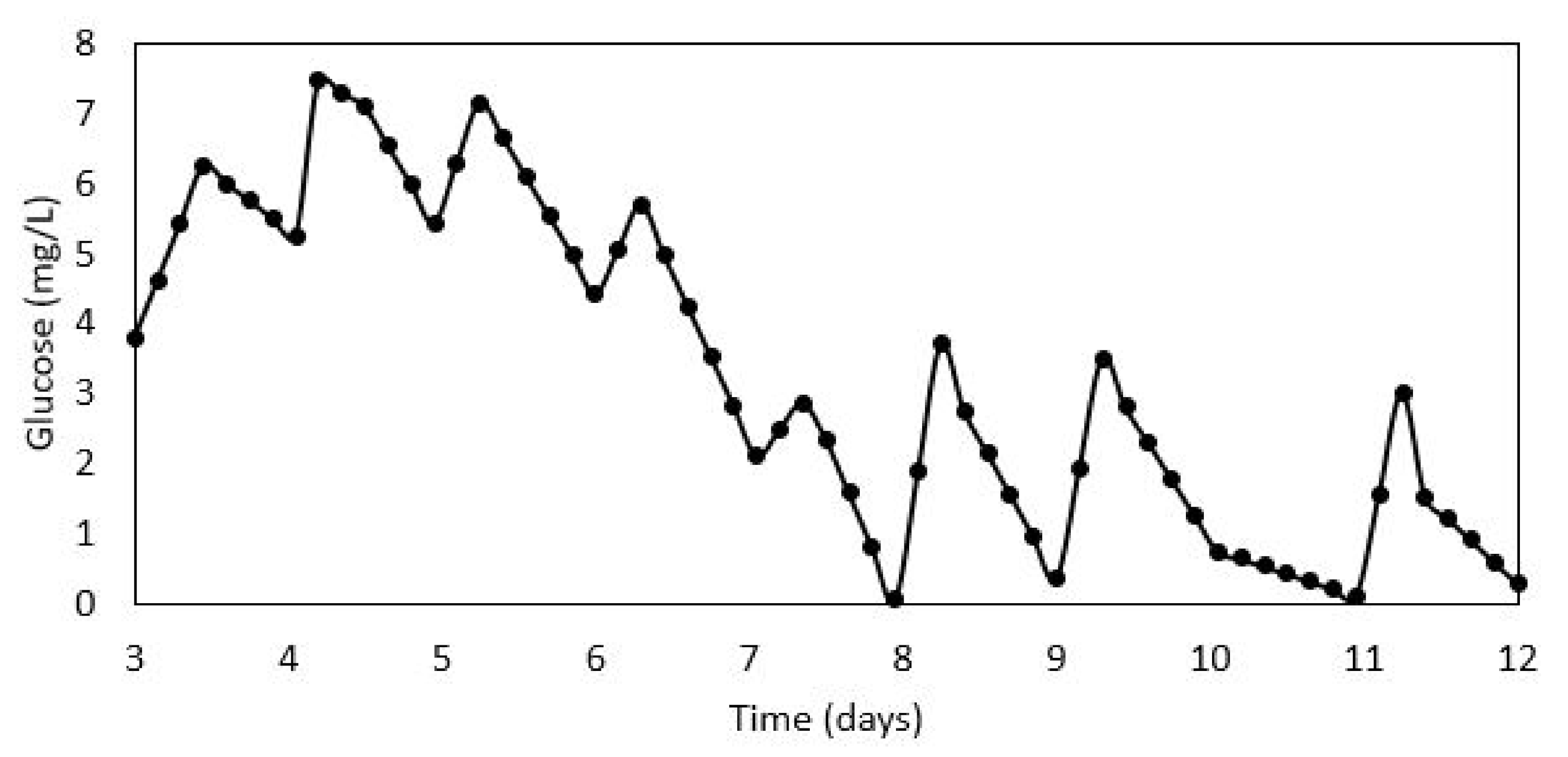
The other more important question is how to utilize the newly computed glucose concentration. Again, there are two alternatives and here one approach is clearly incorrect. The first alternative is to add an additional data point in the batch. Thus, right after the data point before the addition, a new point is added where the value of the glucose measurement is changed, but the value of the other variables is kept the same. While this sounds intuitively right, such a choice would provide the model with false information. In particular, it would suggest to the model that the value of the glucose changed in one sampling time while the others stayed the same. This is counter to what happens in the process in that the value of the glucose jumps instantaneously. 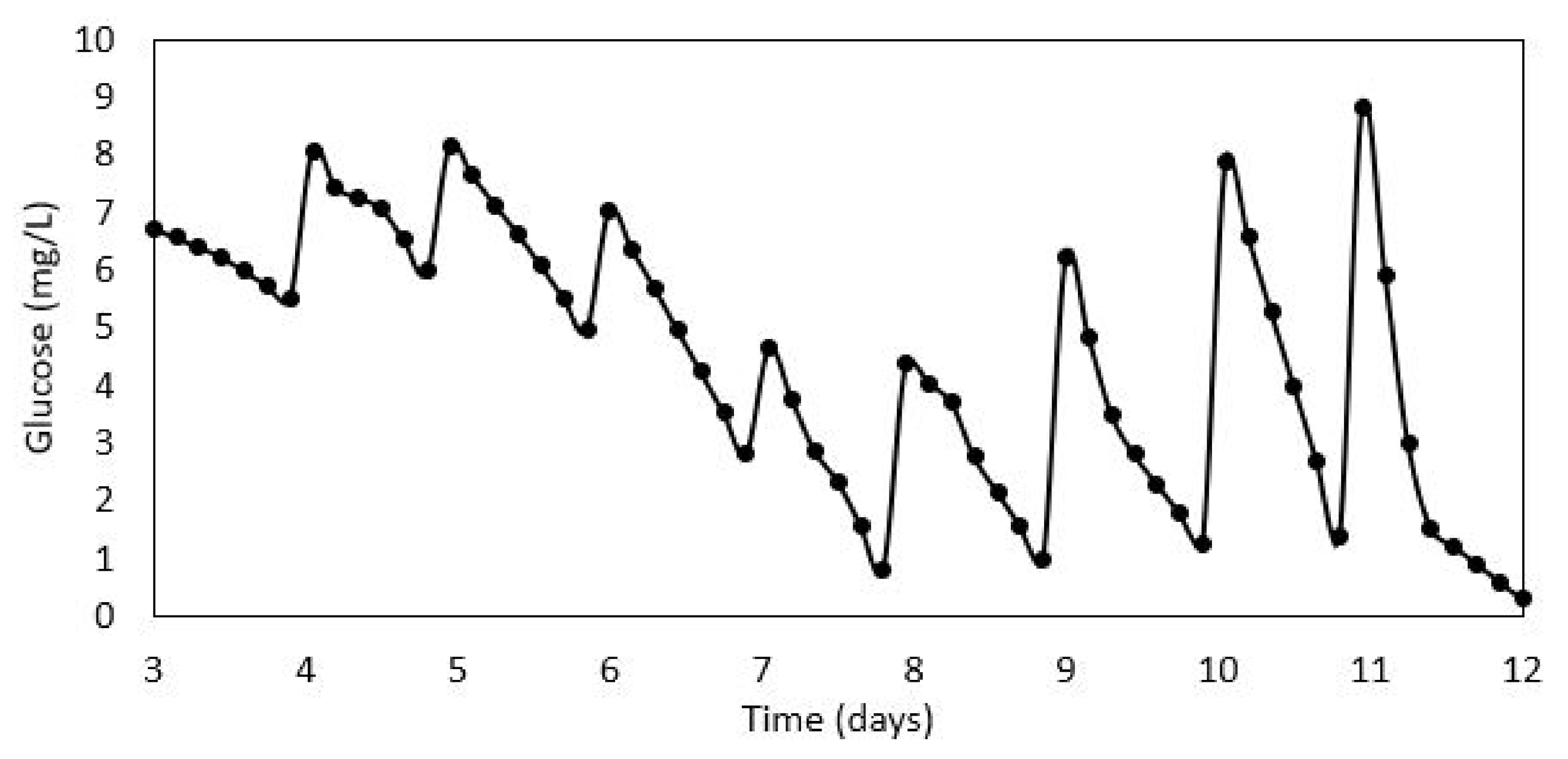The implementation of this approach is shown in Figure 1 and it clearly shows how the concentration in the reactor ‘increases’ between sampling intervals. For example, after Days 3, 6, 7, 8, 9 and 11, the glucose concentration seems to increase slowly over time, which is contrary to what we know happens (i.e., glucose gets consumed). The second and correct adaptation then is to replace the value of the glucose measurement by the newly calculated measurement. As shown in Figure 2, the concentration increases instantly upon glucose addition and the next measured sample shows that the glucose concentration decreases between sampling instances.

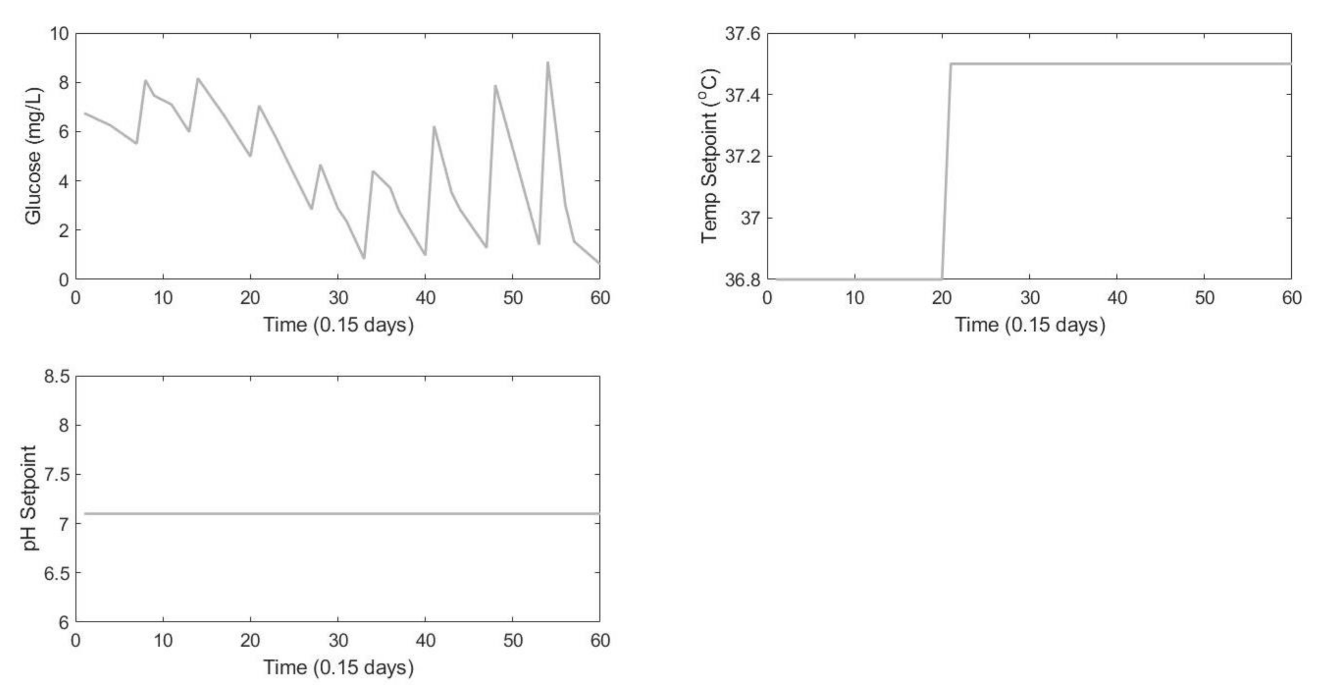
Having determined the right set of inputs and outputs, the training input sequence from one batch is shown below in Figure 3. Note that the temperature and pH setpoints are only moved from the center line values to induce variations in the dataset, reflective of the true process, and as such not all batches have these shifts. To identify the model, data from 11 different batch runs were used for training batches. The training batches were chosen to establish the daily operating conditions of the Sartorius Bioreactor with sufficient variation provided by different temperature and pH setpoint changes providing a reasonably rich dataset.

Remark 1.

We recognize that the use of 11 training batches does limit the ability to accurately validate the model. In future work, as more data become available, the identification can be redone to include more batches. What is perhaps more important to recognize is that the model is good for the data range it is used for in the training. Thus, in conjunction with existing model monitoring techniques [28], one can readily monitor if the model continues to be valid for the batch under consideration. If the monitoring technique reveals that the model predictions are diverging from the observations, the model can be retrained using the new on-line measurements in order to improve model accuracy.

Having handled the discrete nature of the input addition, the data driven modeling approach [24] was subsequently implemented to identify a system model. A state space model of order 3 was identified by ensuring the best model fit during the training stages. The subspace identification approach removes any dependent relationships between the inputs and the outputs; therefore, it is possible to model all of the outputs with only three states using the relationships defined in Equation (1). Note that, while there are several inputs and outputs, the choice in the number of states is determined by the ability of the model to explain the correlations between the past inputs and outputs and the future outputs, and, if some of the outputs observed in the data are co-linear, it might be possible to capture the observed process dynamics using fewer states.

Remark 2.

With regards to the number of states, while it is understood that the process dynamics are nonlinear, what the identified model captures is the process dynamics observed in the training data. In fact, one of the strengths of the subspace identification approach is the ability to determine the number of states in the system (as observed in the data) by utilizing linear algebra based techniques. The first principle model of Karra et al. [2] is an alternate approach to process modeling, one that uses first principles techniques to set up the model structure. In future work, there is the possibility of using the first principles model as a part of a hybrid model structure [29] to better predict the process behavior—such a hybrid model design remains outside the scope of the present work.

The modeling identification procedure [24] used is a combination of subspace identification with PCA and PLS techniques to handle variable batch length missing data problems. The identification approach used in this paper identifies an LTI model as follows: Given s measurements (where s represents the length of the data) of the input $u^{\left(b\right)}\left[k\right]\in {\mathbb{R}}^m$ and the output $y^{\left(b\right)}\left[k\right]\in {\mathbb{R}}^l$ variables from each batch, a model with order n can be identified using the following equations:

$$\begin{array}{c}\hfill \begin{array}{cc}\hfill & {\widehat{\mathbf{x}}}^{\left(b\right)}[k+1]=\mathbf{A}{\mathbf{x}}^{\left(b\right)}\left[k\right]+\mathbf{B}{\mathbf{u}}^{\left(b\right)}\left[k\right],\hfill \\ \hfill & {\mathbf{y}}^{\left(b\right)}\left[k\right]=\mathbf{C}{\widehat{\mathbf{x}}}^{\left(b\right)}\left[k\right]+\mathbf{D}{\mathbf{u}}^{\left(b\right)}\left[k\right],\hfill \end{array}\end{array}$$

(1)

where the objective is to determine the order n, from cross validation, and the system matrices $\mathbf{A}\in {\mathbb{R}}^{n\times n}$, $\mathbf{B}\in {\mathbb{R}}^{n\times m}$, $\mathbf{C}\in {\mathbb{R}}^{l\times n}$, $\mathbf{D}\in {\mathbb{R}}^{l\times m}$.

The system matrices are identified in two stages where first a state sequence is identified and then subsequently the system matrices. The subspace identification approach is carried out using a series of PCA and PLS regressions with non-iterative partial least squares algorithms (NIPALS). The first part of subspace identification is to identify a state trajectory. This is done using PCA by projecting the past inputs and outputs perpendicular to the future inputs. We recognize that the future inputs should be completely independent of any past data, however this step insures we remove any potential correlations as a result of insufficient excitation. Additionally, the future outputs are projected perpendicular to the future inputs. Recognizing that the future outputs are a result of the states and future inputs by removing the correlation between the future inputs the remaining correlation depends on the states. In the next step, PLS is carried out between the newly deflated past inputs and outputs and future outputs. This is done to explain how the past data results in the current states for the future data and to expose the underlying state relationship. Finally, to explicitly identify the state trajectory, where traditional methods [14] utilize singular value decomposition, this approach uses PCA. The end result is a state trajectory that can be used to identify the system matrices using regression techniques. The key use of NIPALS algorithms in these steps gives this approach the ability to handle missing data. For a more detailed explanation of the approach used in this paper, see the work of Patel et al. [24].

Remark 3.

Sartorius has developed a good first principles model of the bioreactor; however, the parameter estimation problem continues to be a focus of future work. That said, the proposed data driven approach could readily be utilized with the first principles model. Thus, a data driven approach which leverages the process data can be utilized to develop a hybrid model for improved prediction power [29].

Remark 4.

One of the considerations when modeling a dynamic process such as cell growth is that there are different phases in cell growth that occur over the course of one batch. The metabolic response of cells to their environment is complex and therefore strongly nonlinear. This response is also widely believed by biologists to be non-Markov (i.e., cells have memory of historical conditions). In these different phases, the process may behave differently making a linear time invariant model an unsuitable choice. To handle this situation, it is possible to treat each different growth phase as a separate smaller batch. This differs from the traditional batch problem since the beginning of each smaller batch represents the end of the previous smaller batch. These smaller batches would then be used as part of the model identification allowing the identified subspace model to appropriately capture the behavior in each phase. As can be seen in the Application Section, the present data driven modeling approach works reasonably well. In future work, as more batches need to be modeled (and the model will likely be utilized for feedback control purposes), such phase-based identification approaches will be pursued. Finally, another direction of generalization would be to determine good initial conditions for the states based on the measured observations. Presently, the states are initialized at a value which is the average of the value for the batches used in training. In future work, an approach can be followed where the subspace model is better initialized for quick convergence of the state observer and the resultant ability to predict starting from early on in the batch.

Remark 5.

Note that one of the advantages of a first principles modeling approach is that it can be more easily extrapolated. Thus if a first principles modeling approach is used, the resultant rate expressions can be utilized to model the operation of the process in a continuous fashion. On the other hand, a data driven model identified using data from batch operation cannot be directly applied to continuous operation. It can serve as a ‘starting point’ and adapted using the monitoring based re-identification approach, and, even more quickly retrained if it is utilized as part of a hybrid modeling strategy via leveraging the extrapolation capability of the underlying first principles model.

3.2. Dynamic Model Validation

This section illustrates the validation procedure for a new batch. Recall that validation is the key step in model identification, by providing a means to evaluate the successes of a developed model. Note that one of the inherent features of any state space based model is the requirement of the knowledge of initial states. If it is a first principles model, where not all the state variables are measured (as is often the case) using the first principles model would require an initial state estimation process step. In the present instance, the model is a linear state space mode, with the states being a realization of the input output dynamics, and thus, by construction, unmeasured. By the same construction, however, the states are observable from the measured outputs, and thus enable the design of a state observer/estimator. Therefore, for a new dataset, an initial state estimate is first computed before prediction is possible. In the present work, a Luenberger observer design is used at the beginning of the batch until the predicted outputs converge with the process outputs. The observer has the following form:

$$\begin{array}{c}\hfill \widehat{\mathbf{x}}[k+1]=\mathbf{A}\widehat{\mathbf{x}}\left[k\right]+\mathbf{B}\mathbf{u}\left[k\right]+\mathbf{L}(\mathbf{y}\left[k\right]-\widehat{\mathbf{y}}\left[k\right])\end{array}$$

(2)

where $\mathbf{L}$ is the observer gain and is chosen to ensure that $(\mathbf{A}-\mathbf{LC})$ is stable.

The missing data problem has specific implication in this regard and needs to be adequately accounted for. Thus, the above observer cannot be ‘implemented’ directly when parts of the output are missing. Specifically, when the output measurement is missing, the term used to update the prediction, $\mathbf{L}(\mathbf{y}\left[k\right]-\widehat{\mathbf{y}}\left[k\right])$, yields an undefined value. To operate the state observer with missing data, this work uses the linearly interpolated value as the process measurement at time k in order to update the states.

Remark 6.

The use of linear interpolation for state estimation is only one of the possible approaches. In addition to multirate state estimation, which is a well documented problem, it possible to build a smaller model without missing data for state estimation. This approach involves building a separate subspace model using the continuous output observations. This model can then be used to estimate the states of the system until they converge and the full model can be used for validation. This approach is not considered in the present manuscript, primarily because of the observed success of the modeling approach, but, with increased data availability and modeling challenges, it could very well be included in future work.

After the states have converged, this is where the identified model’s predictive capabilities are tested with the missing outputs. The remainder of the batch is predicted using the model; however, as the process measurement comes in, the model uses that estimate with the observer in order to update the state estimate at that specific sampling time.

Remark 7.

While the present illustration utilizes linear interpolation for the state estimator, it does not assume any knowledge of the process instead taking measurements as they become available. Linear interpolation is only used to allow for a good state estimate to be obtained which is not a part of validating the identified model’s predictive capabilities. The model is still identified from a dataset with missing values and can be used to predict when process measurements are not available. Note that the model’s predictive capability is not limited to a ‘next step prediction’; the model predicts to the end of the batch and updates the trajectory with each available measurement to predict the final quality more accurately.

To show the effectiveness of the missing data approach on the Sartorius Bioreactor case study, this section identifies a dynamic model used to predict the quality variables and a dynamic model to identify the metabolite rates. These models are built on training data from the Sartorius Bioreactor and then validated on a separate batch. The error is calculated as the normalized prediction error between the predicted model and the true process outputs. Note that the error is only calculated at the points where process measurements are available. The error is calculated as follows:

$$\begin{array}{c}\hfill \begin{array}{c}\hfill PredictionError =\sum \frac{|\widehat{y}-y_{process}|}{predictions}\end{array}\end{array}$$

(3)

where $y_{process}$ represents the process outputs, $\widehat{y}$ represents the predicted outputs and predictions represent the number of available measurements. The identified dynamic model is presented below to show how the output profiles are generated.

$$\begin{array}{c}\hfill \begin{array}{c}\hfill A=\left[\begin{array}{ccc}0.9696& -0.0096& -0.0512\\ 0.0391& 1.0022& 0.0303\\ 0.0314& -0.0308& 0.9724\end{array}\right]\end{array}\end{array}$$

(4)

$$\begin{array}{c}\hfill \begin{array}{c}\hfill B=\left[\begin{array}{ccc}-0.0166& 0.02570& -0.0846\\ 0.01429& -0.0642& 0.3172\\ -0.0311& 0.0115& -0.0385\end{array}\right]\end{array}\end{array}$$

(5)

$$\begin{array}{c}\hfill \begin{array}{c}\hfill C=\left[\begin{array}{ccc}194.8744& 37.6339& 41.8734\\ 0.8548& -0.7058& -0.2336\\ -0.0073& -0.0126& -0.0023\\ 0.0033& 0.0095& -0.0168\\ -0.0363& 0.0219& 0.0483\\ -0.0379& 0.0265& -0.0288\\ 0.0072& 0.0053& 0.0087\end{array}\right]\end{array}\end{array}$$

(6)

$$\begin{array}{c}\hfill \begin{array}{c}\hfill D=\left[\begin{array}{ccc}8.0562& 82.1300& -207.6499\\ -0.0388& -0.1732& 2.8215\\ 0.0006& -0.0028& 0.1480\\ -0.0006& 0.0023& -0.0039\\ -0.00005& 0.0160& -0.0325\\ -0.0007& -0.0171& 0.1315\\ 0.0004& -0.0058& 0.0413\end{array}\right]\end{array}\end{array}$$

(7)

The prediction errors from both the training data and the validation batch are shown in

Table 1. The prediction error between the subspace based model and the process for both the training and validation batches.

Model	Fit Error
Training	0.7930
Validation	1.9696

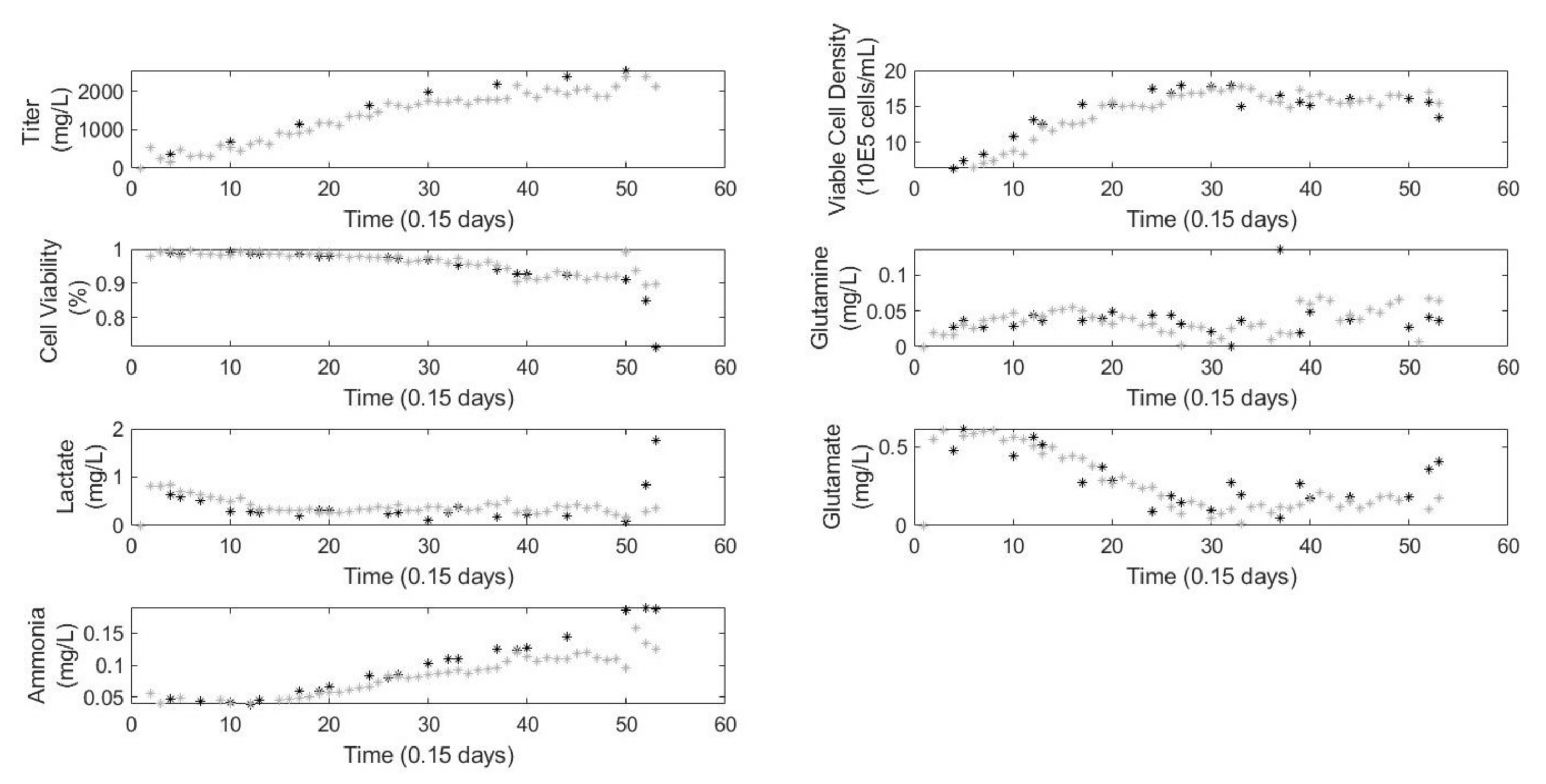
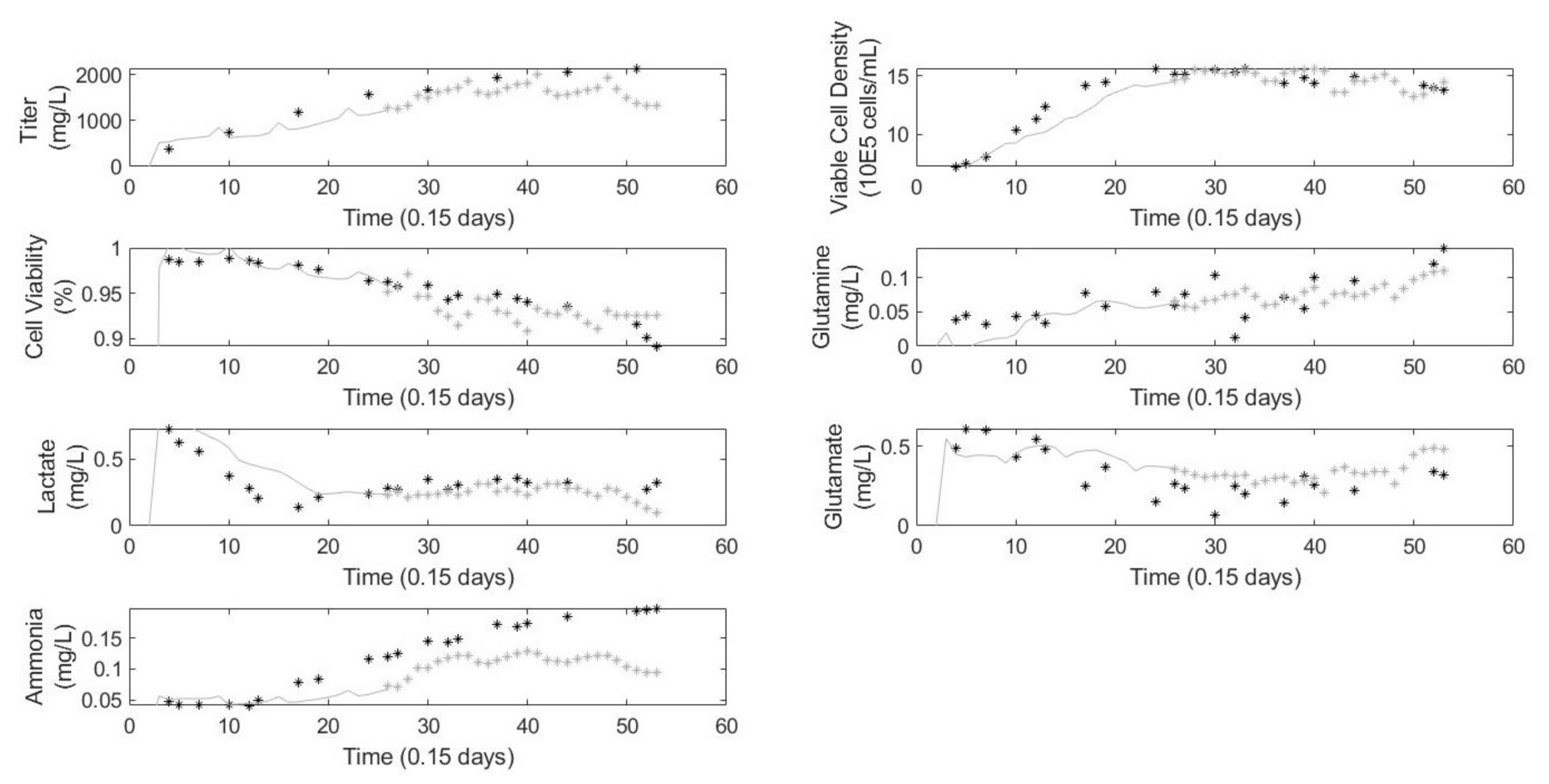
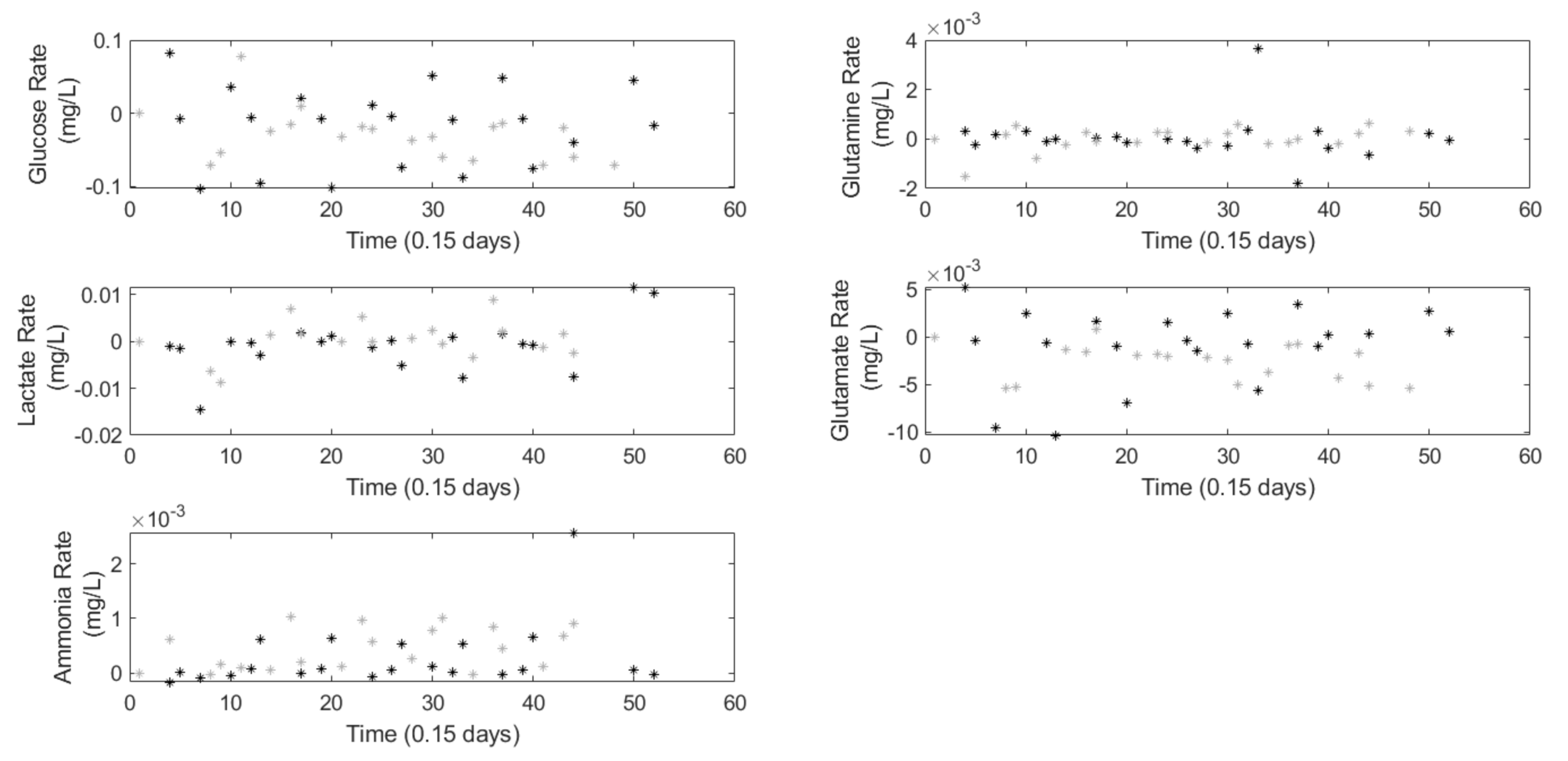
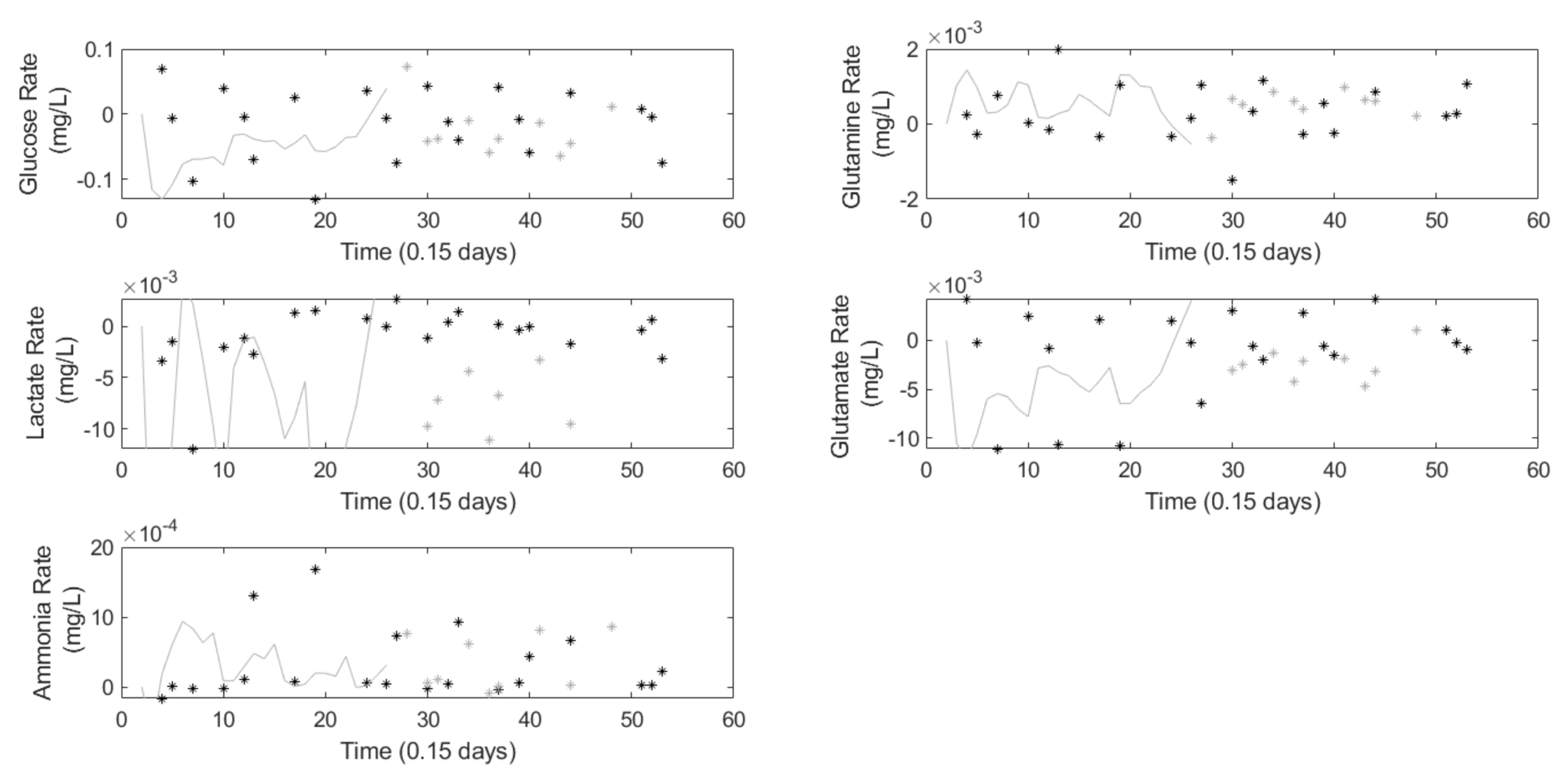
. As expected, the validation error is slightly larger than the training error since the validation batch was not used in model identification. Figure 4 shows the training results and Figure 5 shows the validation results from the quality model. In Figure 4, there are model predictions despite the lack of a process measurement because the model keeps track of the states internally allowing it to make predictions at every time step. As shown in both sets of figures, the model is able to accurately predict the trends in the metabolites and more importantly the viable cell density which shows the cell concentration at the end of the batch. This is the key parameter Sartorius uses in downstream processes, and, despite the large amounts of missing data, the trend was accurately predicted.

4. Metabolite Rate Modeling of the Bioreactor

The metabolite rate model is important for Sartorius in order to see the daily trends in the bioreactor. The goal is to be able to control the reactor overnight based on the end of day predictions. Thus, knowing the trends in the metabolite rates is an important factor when considering what additions need to be before allowing the process to run. In addition to improving the model predictions, knowing the specific metabolite rates is important for ensuring the data driven model matches the physical properties of the system. As described in Section 2.1 the metabolite concentrations have certain effects on the process that must be represented in the data driven model.

4.1. Metabolite Rate Model Identification

The metabolite rates are an important part of the bioreactor process as they determine how the outputs from the dynamic mode change with respect to the viable cell density. Analyzing the metabolite rates is an important part of determining the ideal input conditions required for optimal growth in each stage. The specific metabolite rates are calculated as follows:

$$\begin{array}{cc}\hfill R_{m_t}\left(x_v\right)& =\frac{m_t(t+h)-m_t\left(t\right)}{i{x}_v}\hfill \end{array}$$

(8)

$$\begin{array}{cc}\hfill i{x}_v& =\frac{0.6x_v\left(t\right)+0.4x_v(t+h)}{h}\hfill \end{array}$$

(9)

where $R_{m_t}$ denotes the metabolite rate for a metabolite $m_t$, $x_v$ represents the viable cell density, $i{x}_v$ represents the integrated viable cell density and h represents the sampling interval. The modeling approach calculates metabolite rates using three inputs (glucose concentration, temperature setpoint and pH setpoint) and five outputs (glucose rate, glutamine rate, lactate rate, glutamate rate and ammonia rate), and then builds a model to directly predict the metabolite rates. A metabolite rate model of order 3 was identified based on training fit results. The LTI model is shown below:

$$\begin{array}{c}\hfill \begin{array}{c}\hfill Am=\left[\begin{array}{ccc}0.8655& -0.1089& -0.1605\\ -0.0266& 0.5539& 0.5469\\ -0.0435& -0.4093& 0.7118\end{array}\right]\end{array}\end{array}$$

(10)

$$\begin{array}{c}\hfill \begin{array}{c}\hfill Bm=\left[\begin{array}{ccc}-0.0708& 0.0183& -0.0256\\ -0.0132& 0.1092& -0.5319\\ -0.0915& 0.0259& -0.0620\end{array}\right]\end{array}\end{array}$$

(11)

$$\begin{array}{c}\hfill \begin{array}{c}\hfill Cm=\left[\begin{array}{ccc}0.0048& 0.0191& 0.0061\\ 0.00001& -0.0002& 0.0003\\ 0.0020& 0.0027& -0.0034\\ 0.0006& 0.0015& 0.0004\\ 0.0003& -0.00004& -0.00002\end{array}\right]\end{array}\end{array}$$

(12)

$$\begin{array}{c}\hfill \begin{array}{c}\hfill Dm=\left[\begin{array}{ccc}0.0053& -0.0038& 0.0133\\ 0.0001& -0.0001& 0.0004\\ -0.0006& -0.0005& 0.0024\\ 0.0003& -0.0007& 0.0031\\ 0.00003& 0.00003& -0.0001\end{array}\right]\end{array}\end{array}$$

(13)

4.2. Metabolite Rate Model Validation

The training fit and validation error are shown in

Table 2. The prediction error between the subspace based metabolite rate model and the process for both the training and validation batches.

Model	Fit Error
Training	4.7848
Validation	4.9276

and are similar in magnitude. As shown in Figure 6 for the training data and in Figure 7 for the validation batch, the metabolite rates have a large amount of daily fluctuation. These trends are key to understanding the overnight behavior of the process and the validation fit in Figure 7 shows how the metabolite rate model is able accurately model the rates.

For comparison, the metabolite rates are calculated using the dynamic model, as shown in Figure 8, and compared to the metabolite rates calculated using the measurements. As seen in this figure the rate predictions calculated from the predicted measurements do not match very well with the rates calculated using the measurements themselves. In essence, the errors in the predictions of the variables get much more enlarged when using them in the calculations of the metabolite rate. The calculated rates differ by a magnitude of ten in comparison to the rates calculated based on the measurements. The advantage of directly modeling the metabolite rates is clearly demonstrated as the calculated rate relies on the model predictions of the viable cell density and the metabolites. Thus, small errors in these variables compound resulting in a poor result in the prediction of the metabolite rates. Another drawback of calculating the model parameters is that in the glucose consumption rate. In the modeling approach, glucose is utilized as an input [2]. Therefore, using the calculated parameters to identify the glucose rate is not meaningful when attempting to use this model for control purposes. Given the limitations using calculated rates and the inability to model glucose, the use of a separate model to identify the metabolite rates is necessary.

5. Conclusions

In this study, the problem of identifying a dynamic batch model with large amounts of missing data was solved using a modified subspace identification procedure. The Sartorius Bioreactor problem had multi-rate sampling and also had discrete inputs from the glucose feed additions, which were modeled as instantaneous additions. When comparing the metabolite rate modeling approach to the overall dynamic modeling approach, the results show that modeling the entire process using missing data methods is more accurate. Additionally, the dynamic modeling approach is able to accurately handle the discrete input problem using an instantaneous addition profile. The key is to use the NIPALS algorithms to gracefully handle missing data, allowing for accurate model predictions of the validation batches.

References

1. Van’t Riet, K.; Tramper, J. Basic Bioreactor Design; CRC Press: Boca Raton, FL, USA, 1991. [Google Scholar]
2. Karra, S.; Sager, B.; Karim, M.N. Multi-scale modeling of heterogeneities in mammalian cell culture processes. Ind. Eng. Chem. Res. 2010, 49, 7990–8006. [Google Scholar] [CrossRef]
3. Chusainow, J.; Yang, Y.S.; Yeo, J.H.; Toh, P.C.; Asvadi, P.; Wong, N.S.; Yap, M.G. A study of monoclonal antibody-producing CHO cell lines: What makes a stable high producer? Biotechnol. Bioeng. 2009, 102, 1182–1196. [Google Scholar] [CrossRef] [PubMed]
4. Xie, L.; Wang, D.I. High cell density and high monoclonal antibody production through medium design and rational control in a bioreactor. Biotechnol. Bioeng. 1996, 51, 725–729. [Google Scholar] [CrossRef]
5. Sirois, J.; Perrier, M.; Archambault, J. Development of a two-step segregated model for the optimization of plant cell growth. Control Eng. Pract. 2000, 8, 813–820. [Google Scholar] [CrossRef]
6. Dochain, D.; Perrier, M. Dynamical modelling, analysis, monitoring and control design for nonlinear bioprocesses. In Biotreatment, Downstream Processing and Modelling; Springer: Berlin/Heidelberg, Germany, 1997; pp. 147–197. [Google Scholar]
7. Morel, E.; Tartakovsky, B.; Guiot, S.; Perrier, M. Design of a multi-model observer-based estimator for anaerobic reactor monitoring. Comput. Chem. Eng. 2006, 31, 78–85. [Google Scholar] [CrossRef]
8. Deschenes, J.S.; Desbiens, A.; Perrier, M.; Kamen, A. Multivariable nonlinear control of biomass and metabolite concentrations in a high-cell-density perfusion bioreactor. Ind. Eng. Chem. Res. 2006, 45, 8985–8997. [Google Scholar] [CrossRef]
9. Bernard, O.; Mairet, F.; Chachuat, B. Modelling of microalgae culture systems with applications to control and optimization. In Microalgae Biotechnology; Springer: Cham, Switzerland, 2015; pp. 59–87. [Google Scholar]
10. Mairet, F.; Bernard, O.; Cameron, E.; Ras, M.; Lardon, L.; Steyer, J.P.; Chachuat, B. Three-reaction model for the anaerobic digestion of microalgae. Biotechnol. Bioeng. 2012, 109, 415–425. [Google Scholar] [CrossRef] [Green Version]
11. Hu, B.; Zhao, Z.; Liang, J. Multi-loop nonlinear internal model controller design under nonlinear dynamic PLS framework using ARX-neural network model. J. Process Control 2012, 22, 207–217. [Google Scholar] [CrossRef]
12. MacGregor, J.F.; Jaeckle, C.; Kiparissides, C.; Koutoudi, M. Process monitoring and diagnosis by multiblock PLS methods. AIChE J. 1994, 40, 826–838. [Google Scholar] [CrossRef]
13. Flores-Cerrillo, J.; MacGregor, J.F. Control of batch product quality by trajectory manipulation using latent variable models. J. Process Control 2004, 14, 539–553. [Google Scholar] [CrossRef]
14. Moonen, M.; De Moor, B.; Vandenberghe, L.; Vandewalle, J. On-and off-line identification of linear state-space models. Int. J. Control 1989, 49, 219–232. [Google Scholar] [CrossRef]
15. Qin, S.J. An overview of subspace identification. Comput. Chem. Eng. 2006, 30, 1502–1513. [Google Scholar] [CrossRef]
16. Huang, B.; Ding, S.X.; Qin, S.J. Closed-loop subspace identification: An orthogonal projection approach. J. Process Control 2005, 15, 53–66. [Google Scholar] [CrossRef]
17. Van Overschee, P.; De Moor, B. A unifying theorem for three subspace system identification algorithms. Automatica 1995, 31, 1853–1864. [Google Scholar] [CrossRef]
18. Corbett, B.; Mhaskar, P. Subspace identification for data-driven modeling and quality control of batch processes. AIChE J. 2016, 62, 1581–1601. [Google Scholar] [CrossRef]
19. Larimore, W.E. Statistical optimality and canonical variate analysis system identification. Signal Process. 1996, 52, 131–144. [Google Scholar] [CrossRef]
20. Shang, L.; Liu, J.; Turksoy, K.; Shao, Q.M.; Cinar, A. Stable recursive canonical variate state space modeling for time-varying processes. Control Eng. Pract. 2015, 36, 113–119. [Google Scholar] [CrossRef]
21. Van Overschee, P.; De Moor, B. N4SID: Subspace algorithms for the identification of combined deterministic-stochastic systems. Automatica 1994, 30, 75–93. [Google Scholar] [CrossRef]
22. Verhaegen, M.; Dewilde, P. Subspace model identification part 2. Analysis of the elementary output-error state-space model identification algorithm. Int. J. Control 1992, 56, 1211–1241. [Google Scholar] [CrossRef]
23. Markovsky, I. Exact system identification with missing data. In Proceedings of the 52nd IEEE Conference on Decision and Control, Florence, Italy, 10–13 December 2013; pp. 151–155. [Google Scholar]
24. Patel, N.; Nease, J.; Aumi, S.; Ewaschuk, C.; Luo, J.; Mhaskar, P. Integrating Data-Driven Modeling with First-Principles Knowledge. Ind. Eng. Chem. Res. 2020, 59, 5103–5113. [Google Scholar] [CrossRef]
25. Wang, J.; Qin, S.J. A new subspace identification approach based on principal component analysis. J. Process Control 2002, 12, 841–855. [Google Scholar] [CrossRef]
26. Jiang, Q.; Yan, X.; Huang, B. Performance-driven distributed PCA process monitoring based on fault-relevant variable selection and Bayesian inference. IEEE Trans. Ind. Electron. 2015, 63, 377–386. [Google Scholar] [CrossRef]
27. Corbett, B.; Mhaskar, P. Data-driven modeling and quality control of variable duration batch processes with discrete inputs. Ind. Eng. Chem. Res. 2017, 56, 6962–6980. [Google Scholar] [CrossRef]
28. Kheradmandi, M.; Mhaskar, P. Adaptive Model Predictive Batch Process Monitoring and Control. Ind. Eng. Chem. Res. 2018, 57, 14628–14636. [Google Scholar] [CrossRef]
29. Ghosh, D.; Hermonat, E.; Mhaskar, P.; Snowling, S.; Goel, R. Hybrid modeling approach integrating first-principles models with subspace identification. Ind. Eng. Chem. Res. 2019, 58, 13533–13543. [Google Scholar] [CrossRef]
Figure 1. The glucose input profiles for a training batch using the incorrect assumption of taking measurements whenever they are sampled.
Processes 08 01686 g001
Figure 2. The glucose input profiles for a training batch using the correct approach of updating the glucose concentration instantaneously.
Processes 08 01686 g002
Figure 3. The input profiles for a training batch.
Processes 08 01686 g003
Figure 4. The training fit (grey) from the dynamic model for each output are compared against the process data (black) for a training batch.
Processes 08 01686 g004
Figure 5. The process data (black) is compared with the dynamic model predictions using the state observer (grey solid) until the states converge and then the dynamic model predicts the remainder of the validation batch (grey starred).
Processes 08 01686 g005
Figure 6. The output predictions (grey) from the metabolite model for each output are compared against the process data (black) for one training batch.
Processes 08 01686 g006
Figure 7. The process data (black) is compared with the metabolite rate model predictions using the state observer (grey solid) until the states converge and then the metabolite rate model predicts the remainder of the validation batch (grey starred).
Processes 08 01686 g007
Figure 8. The process data (black) is compared with the model predictions batch (grey starred).
Processes 08 01686 g008