Multiscale Modeling and Recurrent Neural Network Based Optimization of a Plasma Etch Process


College of Control Science and Engineering, Zhejiang University, Hangzhou 310027, China
*
Author to whom correspondence should be addressed.
Processes 2021, 9(1), 151; https://0-doi-org.brum.beds.ac.uk/10.3390/pr9010151
Submission received: 15 December 2020
/
Revised: 7 January 2021
/
Accepted: 11 January 2021
/
Published: 14 January 2021
(This article belongs to the Special Issue Modeling, Control, and Optimization of Batch and Batch-Like Processes)
Abstract
:In this article, we focus on the development of a multiscale modeling and recurrent neural network (RNN) based optimization framework of a plasma etch process on a three-dimensional substrate with uniform thickness using the inductive coupled plasma (ICP). Specifically, the gas flow and chemical reactions of plasma are simulated by a macroscopic fluid model. In addition, the etch process on the substrate is simulated by a kinetic Monte Carlo (kMC) model. While long time horizon optimization cannot be completed due to the computational complexity of the simulation models, RNN models are applied to approximate the fluid model and kMC model. The training data of RNN models are generated by open-loop simulations of the fluid model and the kMC model. Additionally, the stochastic characteristic of the kMC model is presented by a probability function. The well-trained RNN models and the probability function are then implemented in computing an open-loop optimization problem, in which a moving optimization method is applied to overcome the error accumulation problem when using RNN models. The optimization goal is to achieve the desired average etching depth and average bottom roughness within the least amount of time. The simulation results show that our prediction model is accurate enough and the optimization objectives can be completed well.
1. Introduction
Plasma etch has been applied in the manufacturing of integrated circuits (IC) for over 50 years, and becomes even more essential due to the continuous decreasing of the fabricating scale [1,2]. The traditional “failures and corrections” experimental procedure is not enough to maintain and develop the plasma etch technique. In addition, therefore, simulation of plasma etch is an effective way to improve our understanding about the etching process and to help improve the process technique [3,4]. A lot of work has been done to simulate the gas flow and chemical reactions in the plasma chamber, and there are three main types of models: kinetic model, fluid model, and hybrid model. Fluid model is the most commonly used model because of its computational efficiency and flexibility in coupling the electromagnetic fields. Additionally, the complex transport phenomena and reactions which motivate the etching process are simulated by some quite precise approaches, like level set method and kMC method. Level set method is based on solving a Hamilton–Jacobi type equation for a level set function, which has stable, accurate, and efficient performance in dealing with interface evolution problems with sharp corners, change topology, and order of magnitude changes in speed [5,6], while, in order to realize a high resolution simulation of plasma etch process, kMC is the most potential method for which it has both an atom resolution and the ability to deal with relatively long-time scales [7,8,9]. An appropriate modeling methodology is established by the fact that kMC transforms every physical phenomena into stochastically selected events. The key step for kMC method is to attain the probability table of the simulated process through simulations or experiments.
The natural disparate scale between the macroscopic plasma chamber and the microscopic etching process prevent us from simulating the plasma behavior and the etching process concurrently. Continuous models used to simulate plasma are insufficient on the microscopic scale. Meanwhile, the approaches employed on the simulating etching process, like kMC, are too computationally expensive to apply on macroscopic domains. Fortunately, advances in high-performance computing have made it possible to address this issue with the multiscale method. Such methods were developed in particle transformation [10,11], thin film growth [12], braided composites [13], cracked concrete [14], and the plasma-enhanced chemical vapor deposition (PECVD) process [15]. Through the coupling bridges of heat, particle, or energy, the microscopic model and the macroscopic model are computed concurrently in these works. Nevertheless, few works have developed the three-dimensional multiscale model for the plasma etch process. In the earlier work of our group, we have presented a multiscale model for the silicon etch process using Cl/Ar inductive coupled plasma (ICP) [16].
However, this multiscale system is too computationally expensive for long time horizon optimization due to the computational complexity of the fluid model and kMC model. Using data driven models like machine learning models to approximate these computationally expensive models through system identification could be a potential solution. System identification is widely applied in many fields of engineering [17,18]. Machine learning methods were first used in system identification in 1990, and showed great performance in this area [19,20]. Moreover, the machine learning and deep learning methods have grown rapidly in the last 20 years thanks to the development of advanced machine learning algorithms, innovative neural network structures, powerful computers, and open-source software libraries. Among all of these machine learning methods, RNN has been widely applied for approximating nonlinear dynamical systems. RNN was first proposed in the 1980s, when Hopfield networks were first created for pattern recognition [21]. In addition, later, long Short-Term Memory (LSTM) and gated recurrent unit (GRU) were invented to overcome the gradient vanishing problem of RNN [22,23]. What distinguishes RNN from the commonly known feedforward neural networks is the existence of close cycles in the connections topology. These cycles make it possible for RNN to capture the dynamic behavior of the nonlinear system [24]. From literature, a theorem is given that RNN can approximate any dynamic system to arbitrary accuracy [25]. Several works about using RNN to approximate dynamic systems have already been done: taking a discrete-time approach [26] or a continuous time approach [27]. Thus, RNN is a suitable approach to approximate the fluid model and the kMC model in our multiscale system.
Motivated by all of the above, we focus on the development of a multiscale modeling and RNN based optimization framework of the plasma etch process on a silicon substrate with uniform thickness using Cl/Ar ICP. The plasma domain is simulated by a continuous fluid model, which is constructed and computed by COMSOL Multiphysics (for the convenience of writing, the following is called COMSOL). In addition, the etch process is simulated by a kMC model. Then, RNN models are applied to approximate the fluid model and the kMC model in order to reduce the computational complexity. The training data of RNN models are generated by open-loop simulations of the fluid model and the kMC model. Additionally, the stochastic characteristic of the kMC model is described by a probability function. The RNN models and the probability function are then implemented in computing an open-loop optimization problem, in which a moving optimization method is applied to overcome the error accumulation problem when using RNN models. The optimization goal is to achieve the desired average etching depth and average bottom roughness within the least amount of time. The simulation results show that our prediction model is accurate enough and the optimization objectives can be completed well.
The rest of the article is organized as follows: first, the muitiscale modeling process is presented. Then, the prediction model that includes the RNN models and the probability function is presented. In addition, then the optimization problem is elaborated. In the end, the simulation results are shown and discussed.
2. Multiscale Model
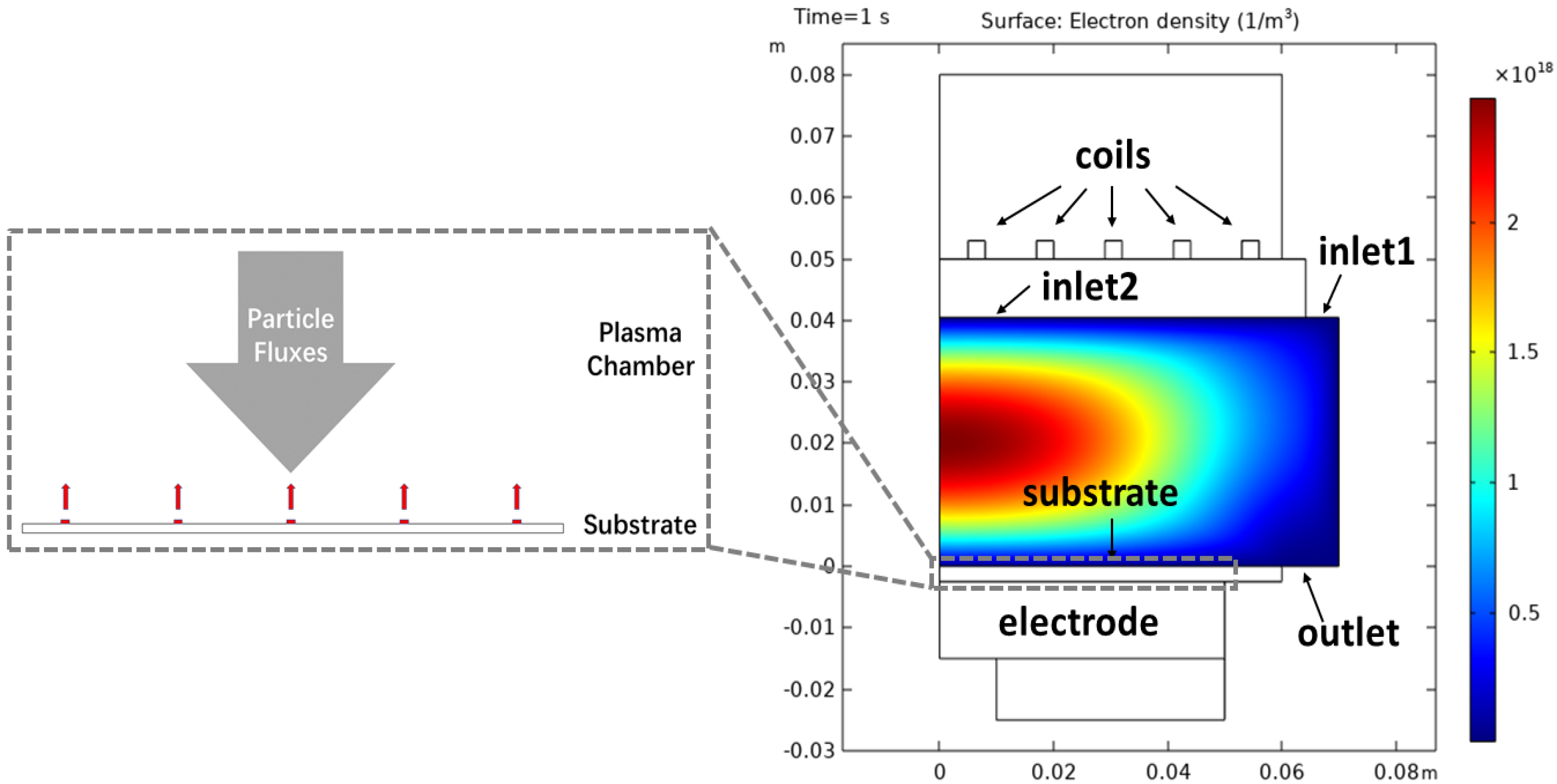
The plasma reactor considered in this work is shown in Figure 1. A two-dimensional model can be used due to the cylindrical symmetry of ICP. The reactive gases enter the chamber through two inlets: the edge inlet (inlet1) and the center inlet (inlet2), and then the top coils generate and maintain the plasma (an electrically neutral mixture of molecules, atoms, ions, electrons, and photons). Ions are accelerated by the bottom electrode and bombard on the substrate, which is placed on top of the electrode. With chemical reactions, ion impact reactions, and particle transportation, the nanoscale etching process occurs on the substrate, and desorbed atoms are pumped out of the plasma domain.
As is shown in Figure 1, the plasma is generated in a macroscopic chamber, while the etching process that occurs on the substrate is at the nano scale. It is quite a necessity to capture both the macroscopic plasma behavior and the microscopic etching behavior. Thus, a multiscale model that consists of two simulation models is presented: the continuous fluid model that describes the gas flow and chemical reactions in plasma chamber is established in COMSOL; and the kMC model that simulates the kinetic behavior of the etching surface is completed through C language. A spatial-temporal discrete method is applied to address the issue of computing the fluid model and the kMC model concurrently. The spatial discrete method is shown in Figure 1. The whole substrate is divided into several parts, and the fluxes data of each parts are considered uniform. In our pre-test, we find that the flux data are quite different in different parts of the substrate. Three is the lowest number that the substrate should be divided for that the discrete parts should reflect the flux data on the middle and two sides of the substrate. Considering the computational efficiency and our model complexity, we choose to divide the whole substrate into five parts. The etch process of each parts is calculated by one kMC model. Furthermore, the data exchanges between the macroscopic model and the microscopic model are operated in every time step . The following sections present both the macroscopic fluid model and the microscopic kMC model.
2.1. Macrosopic Model
Basically, there are three main modules in computing the macroscopic fluid model: the Maxwell equations, the drift–diffusion equations and the heavy species transportation equations (simplified Stefan–Maxwell equations). The electromagnetic field that spread all over the plasma etch equipment is solved through the computing of Maxwell equations. Furthermore, the electron density and the electron energy density are solved through the computing of drift–diffusion equations. In addition, all the heavy species (neutral particles and ions) densities are solved through the computing of heavy species transportation equations. All of these equations are partial differential equations and thus can be solved by the finite-element methods.
Specifically, the gas mixture in plasma chamber would be Cl and Ar. Twelve species and their corresponding reactions are taken into account. Four excitation forms of Cl are included: ClV, Cl(B3PI), Cl(C1PI), and Cl(B3PI+C1PI). ClV is generated by vibration excitations and the latter three are generated by electronic excitations. The excited energy of these four species are 0.068 eV, 2.5 eV, 3.12 eV, and 9.25 eV, respectively. Cl is generated by attachment, and this negative ion owns a very small percentage of all ions. Two ionization reactions are computed and the reaction products are Cl and Cl, respectively. In addition, both of their ionization energies are 11.48 eV—while only one excited form of Ar is considered, which is Ars (excitation energy is 11.5 eV). In addition, one ionic species Ar (ionization energies are 15.8 eV and 4.24 eV) is taken into account. The reactions of these species are divided into three types: electron impact reactions, heavy species reactions, and wall reactions. The excited species and ions are all generated by ion impact reactions, which makes it the most important part in the plasma chemistry. The heavy species reactions happen when two heavy particles impact and react to form a new particle. Wall reactions occur when particles impact on the plasma chamber wall. We note that the latter two types of reactions would transform the excited species and ions to the ground state species. All of the reaction coefficients and reaction rates can be found in [28,29,30,31].
2.2. Microscopic Model
The kMC method applied in this work follows closely our former work [16] and share many similarities with other commonly used Monte Carlo methods. The details will not described again in this article. In addition, in order to show the completeness of the modeling process, we will present the main structure of the kMC model.
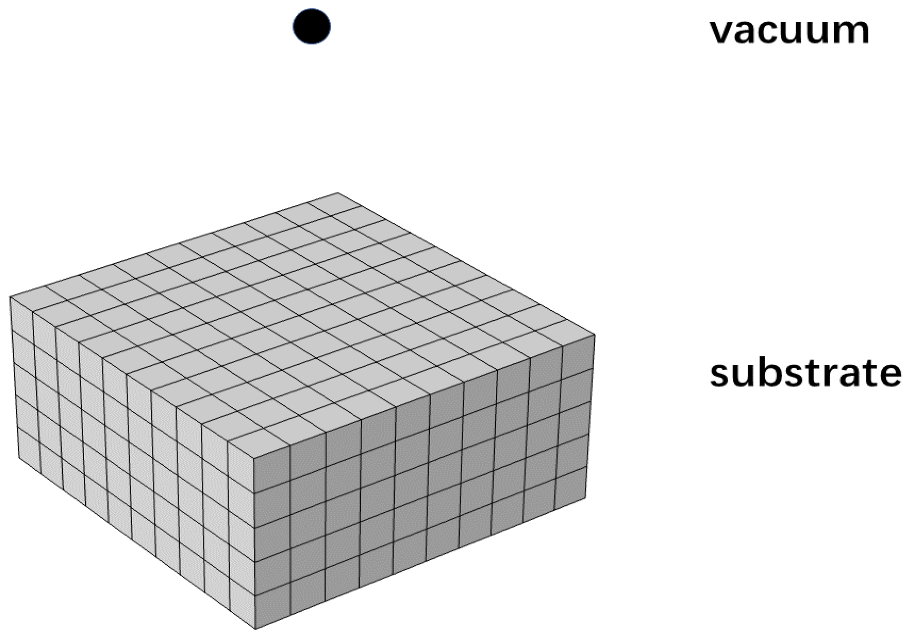
The KMC method uses stochastically selected events to represent all the phenomena of etching process, and realize a kinetic simulation. In Figure 2, we show the simplified schematic diagram of the virtual simulation box. The lattice, representing the substrate, consists of atomic cubic cells, and each of them would only include one atom. The side length of each cube is set as , where is the atomic density of the substrate material. The black sphere above the lattice represents the particles from the plasma region. When it bombards onto the lattice surface, the etching parameters are calculated based on the material type, injection angle, and local coverage type. The atomic kinetic simulation is realized by adding or removing atoms on the lattice. In this work, the substrate material would be silicon. In addition, the resist material can be set as incorruptible since the sputtering rate of etchable resist is relatively low. Specifically, the initial structure of the lattice would be: the size of the microscopic silicon lattice is 100 × 100 × 100 monolayers (ML); the resistive mask is placed above the substrate and the height of the resistive mask would be 50 ML; a 40 × 40 ML surface is uncovered by the resistive mask and is placed in the middle of the whole surface.
2.2.1. Simulation Methods
The particle transportation process in vacuum is computed by the three-dimensional injection trajectories. First, when one particle from plasma injects into the simulation box, the particle type is selected based on the compared results between the flux data from plasma and a random number. In addition, the initial inject location is chosen as a randomly allocated point of the interface between the plasma domain and the simulation box. We note that only one particle would be simulated in one time step, and the transportation process is assumed without any collision, which is commonly assumed in the high vacuum process where the mean free path is large. Then, the angular functions of different fluxes are given, and the incident angles are randomly sampled from these functions. The expressions of these functions are based on in situ plasma measurements and are given in [32,33].
When particles reach the substrate surface, two types of reactions occur. Neutral particles from the plasma domain that have the energy order can participate in the chemical reactions with surface atoms. The chemical reaction probabilities can be found in [31,34], and will stored in a reaction matrix. When a neutral particle reaches one surface cell, the corresponding reaction probability will be found in the reaction matrix and compared to a random number P = rand(0,1). If reactions occur, surface atoms will desorb or be replaced. The ions accelerated by the bottom electrode have the energy order , and will etch the substrate physically, like sputtering and ion-enhanced etching. We note that the physical etching rate is much larger than the chemical etching rate. In our case, the chemical etching rate is nearly zero due to the nonvolatile character of the chemical reaction product, while they can be sufficiently removed by ion enhanced etching. Meanwhile, the surface atoms can also be removed through physical sputtering. The etching yield expressions of ion-enhanced etching and sputtering can be found in [3,35,36]. When an ion impacts on one surface cell, the number of surface atoms that are etched is determined by the average etching field of its neighbor cells and itself.
The injected particle will be reflected to vacuum again if no surface reactions happen until it reacts or moves out of the simulation box. The desorbed etch products, which are generated by surface reactions, will re-emit to the vacuum until they reach the substrate surface or move out of the simulation box. Etch products can deposit on the substrate surface and the deposition probabilities can be found in [31]. The etch products will be reflected to vacuum again if no depositions happen until they deposit or move out of the simulation box.
2.2.2. Numerical Algorithm of the Model
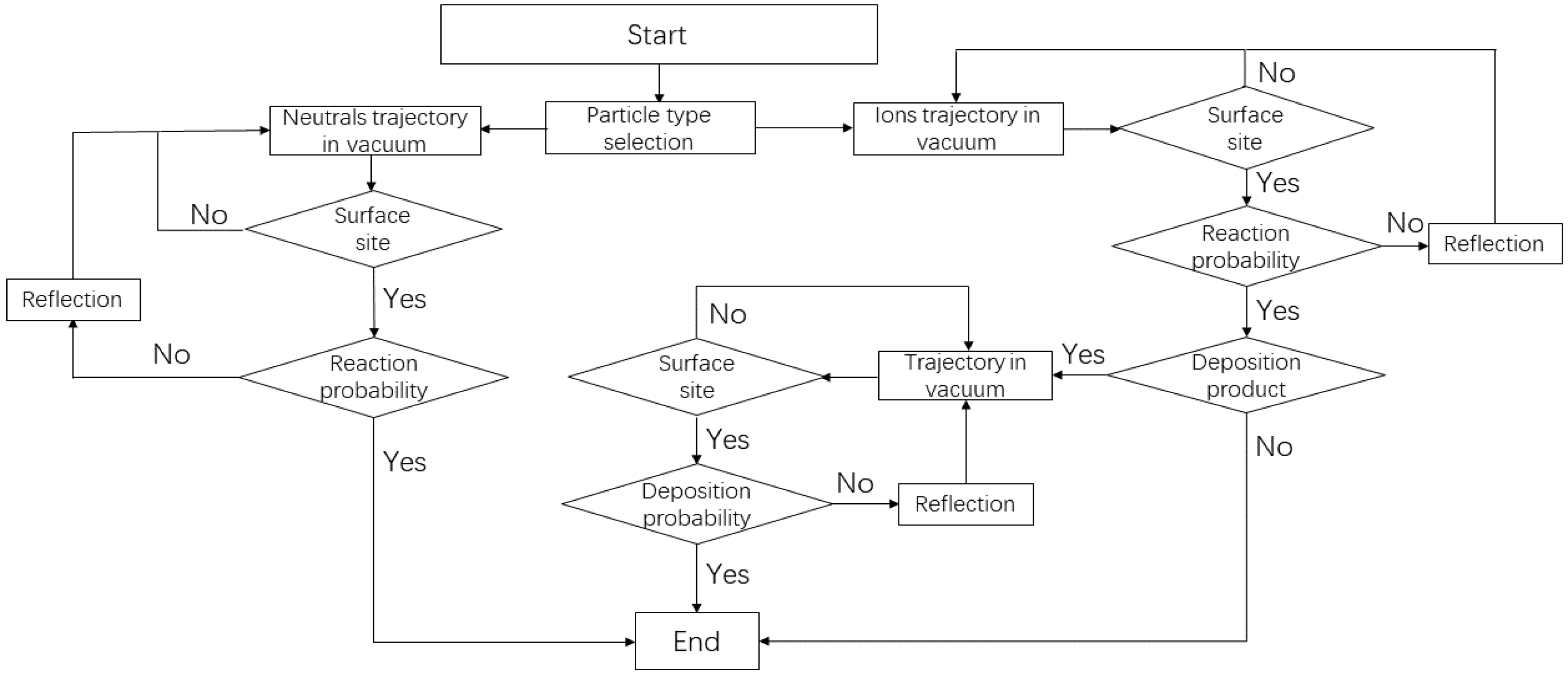
At the beginning of every step, the particle type is selected based on the flux data that come from the plasma model. Then, the injection trajectory is computed based on the selection of the particle initial position and the injection angle. When all the simulative particles and etch products have reacted with surface atoms or moved out of the simulation box, one simulation step ends. A periodic boundary condition is used in the sidewalls of the simulation box. In addition, a perfectly absorbing boundary is applied on the interface between the simulation box and the plasma, which means all particles and etch products would not be computed again when they reach the boundary. The flowchart of the numerical algorithm of the microscopic model is shown in Figure 3.
3. Prediction Model Establishment
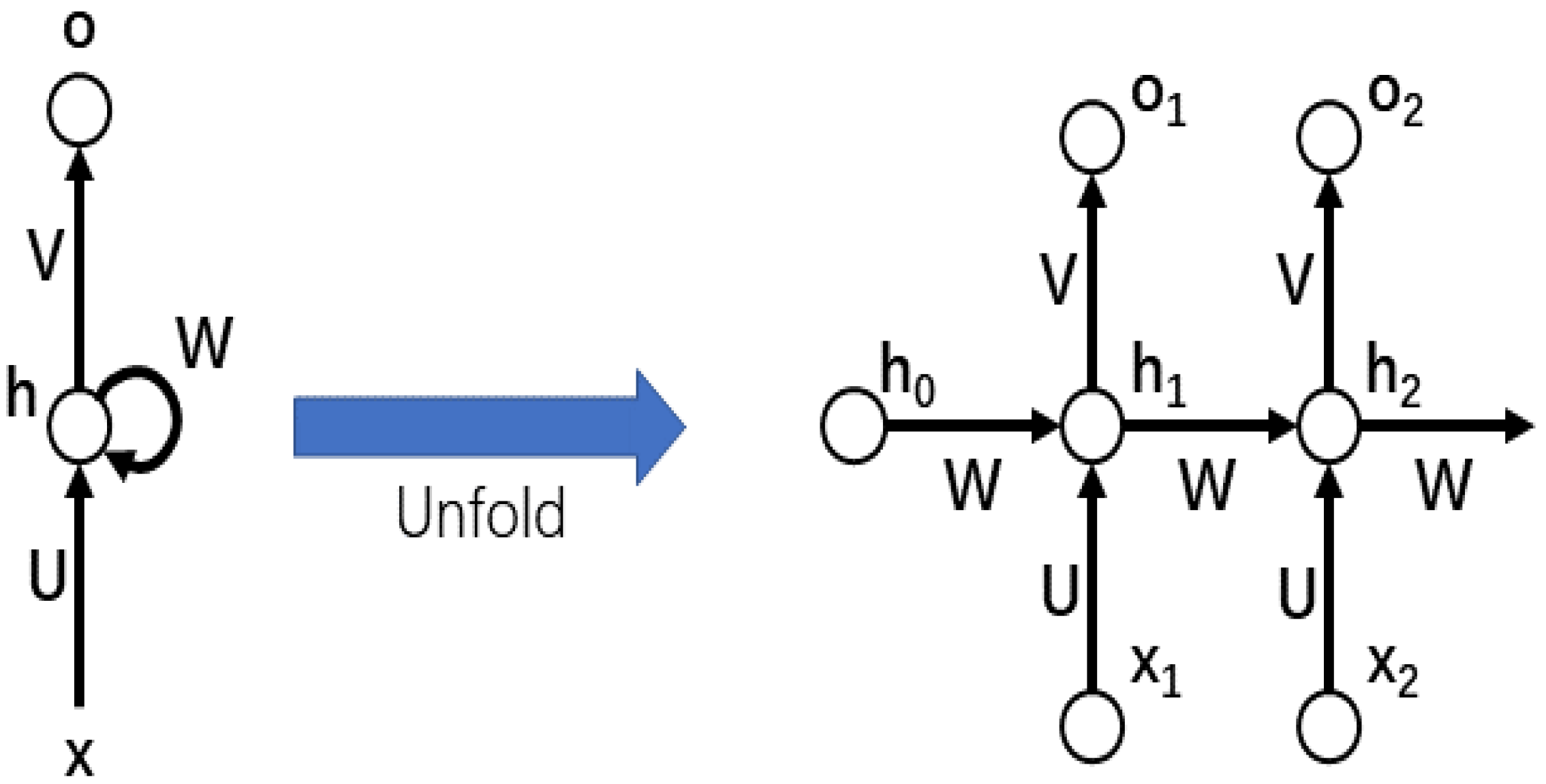
With the fluid model and the kMC model, we have established the multiscale model of the plasma etch process. However, long time horizon prediction and optimization are too computationally expensive by using the fluid model and the kMC model. The fluid model and the kMC model are all nonlinear models with dynamic behaviors, while RNN can also describe nonlinear dynamic behaviors since it has the memory of past states. As is shown in Figure 4, the states derived from past inputs are imported into the next RNN cell, which shows the dynamic behavior. Through the open source software like pytorch and tensorflow, RNN can be easily established. In addition, thanks to the recent development of parallel computing acceleration technique of GPU, the training process of RNN can be quite efficient. Thus, RNN is an appropriate approach to address our issue.
In the following parts, we will present the data generation process and the training process of the applied RNN models. From previous work, the theorem is given in which RNN can approximate any dynamic system to arbitrary accuracy [25]. However, it should be noted that RNN models are nonlinear models without stochastic characteristic, which means that the computation results under the same initial condition and inputs would be constant. Thus, using simple RNN models as the prediction model cannot capture the natural stochastic characteristic of the kMC model. In this article, a probability function is analyzed to describe this important part in the microscopic kMC model. The data for training and analyzing are from the open-loop simulations of the fluid model and the kMC model. In order to capture all the system dynamic behaviors, the open-loop simulations should be operated with a combination of different initial states and input values. In addition, the data are sampled at discrete time steps. Two RNN models will be presented to approximate the fluid model and the kMC model, respectively. To distinguish these two RNN models, the RNN model that approximated the macroscopic fluid model is named RNN, and the other one is named RNN. We will separately illustrate the data generation process and training process of the RNN model and the RNN model.
3.1. Macroscopic Model
3.1.1. Data Generation
As we mentioned in Section 2, the inputs of the fluid model would be: Ar/Cl ratio of the input gas at edge inlet (), Ar/Cl ratio of the input gas at center inlet (), the power of the top coils (), and the bottom electrode bias (). In addition, the outputs would be the particle flux data on the interface of the fluid model and the kMC model, which is noted as (i is the particle type number and k is the location number). The sampling period of the fluid model open-loop simulation would be = 0.2 s. We note that this time step is enough for the plasma states to coverage from any different initial states to the final states. Thus, we only need to consider the selection of the inputs. Specifically, the inputs are selected randomly at the beginning of every time step, and the selection range of each inputs would be: , , 800 W W, 50 V V. The data are finally obtained from an open-loop simulation which includes the 800 sampling periods.
3.1.2. Training Process
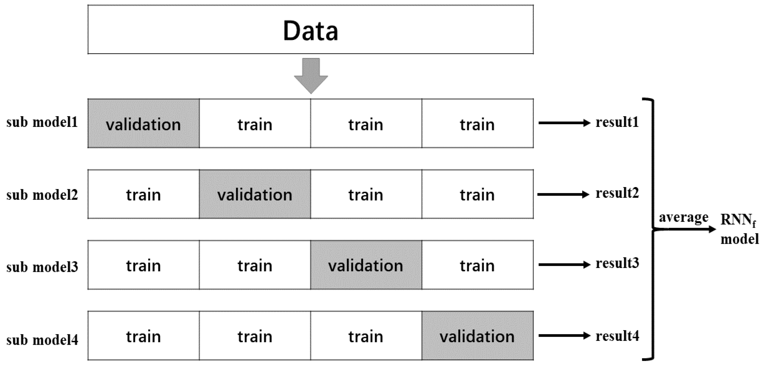
The inputs of RNN would be the values of , , , and at every time step (). The outputs of RNN are the values of after a simulation. The RNN model is constructed by the RNN module of pytorch. The python version is 3.0, the torch version is 1.2.0, and the cuda version is 10.0. The GPU that is used for training is GTX 1080ti. We use the k fold cross validation method to establish four sub RNN models. In addition, an ensemble method is used: the RNN model would be the ensemble of these four sub RNN models. The training process of these four sub RNN models and the RNN model is shown in Figure 5: four sub RNN models are trained, and the RNN model is the average of these four sub models. The validation data are not used for training the sub models. We note that using the ensemble of multiple RNN models can improve the model prediction accuracy and capture more system dynamic behaviors. The parameters of these four sub models like neuron numbers and layer numbers are determined by the grid search method. Specifically, there will be four layers in the recurrent layer and two linear layers as well as one Rectified Linear Unit (ReLU) layer in the output layer. The parameter optimization algorithm is the Adam optimization method. The loss function is mean square error (MSE). In order to avoid the over-fitting problem, the training process would be finished if the loss falls below the desired threshold (which is set to be 10). The inputs and outputs data are normalized by the maximum and minimum values of each variable:
where is the jth variable of the data, and and are the maximum and minimum values of the jth variable.
3.2. Microscopic Model
We note that the kMC model is a nonlinear model with a stochastic feature. While RNN is not suitable to capture the stochastic feature, we use RNN to approximate the expectation of the kMC model. The stochastic feature is described by a probability function that is analysed based on the open-loop simulation data. The following parts will present the establishment process of the RNN model and the probability function.
3.2.1. Data Generation
As we mentioned in Section 2, the inputs of the kMC model are the particle flux data from the plasma model () and the bottom electrode bias (). The outputs of the kMC model should be the surface topology structure of the lattice. Thus, the height data of the 40 × 40 ML uncovered surface sites are sampled as the output data. The sampling period would also be set as t = 0.2 s. Then, the training data are generated through a 150 run open-loop simulation of the kMC model. The initial condition of each simulation is set as the same as the initial condition mentioned in Section 2.2. The operation time is set as 15 s, thus 75 sampling periods are included in each simulation, and the size of the training data would be 150 × 75 = 11,250. At the beginning of each sampling period, the inputs are randomly selected from the pre-tested ranges (these ranges should be consistent with the simulation results of the fluid model).
In order to analyze the stochastic characteristic of the kMC model, multiple run simulation under the same initial condition and inputs should be operated. Thus, we use the same method as above to generate the open-loop data; only the kMC model is operated 100 times instead of one time in each sampling period. A 20 run open-loop simulation is carried out, and the data size would be 40 × 75 × 100 = 300,000.
3.2.2. Training Process
We note that RNN is applied to approximate the expectation of the microscopic model. Thus, the training data should be the average data of multiple runs open-loop simulation under the same initial condition and inputs, while, from pre-experiments, we found that the RNN model trained by using the single run open-loop data and the RNN model trained by using the average of multiple run open-loop data are quite similar. Thus, we can directly use the single run open-loop data to train the RNN model. The inputs of RNN are the values of and at every time step . The initial hidden states of RNN are the initial surface topology structure (the height data of the 40 × 40 mL uncovered sites) of the kMC model. The outputs are the final surface topology structure of the kMC model after a etch process. The parameters of RNN like neuron number and layer number are determined by the grid search method. The neuron numbers of RNN would be much larger than those of RNN because the inner state and output state dimensions of RNN are much larger than those of RNN. Specifically, there is one layer in the recurrent layer and four linear layers as well as three Rectified Linear Unit (ReLU) layers in the output layer. The training and computation time of the RNN model would be relatively long and therefore the ensemble method would not be applied here. The other settings of the training process are the same as the RNN model.
3.2.3. Stochastic Characteristic Analysis
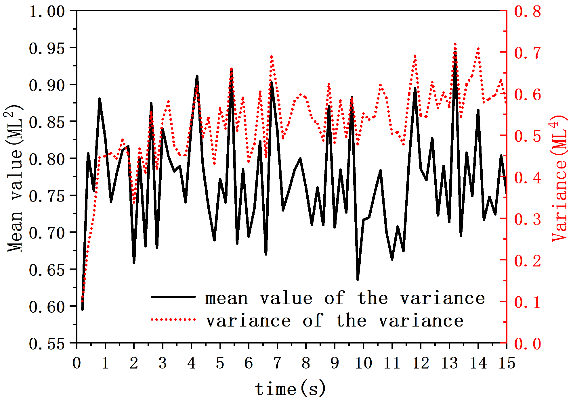
Due to the stochastic characteristic of the kMC method, the height of the lattice surface sites will stochastically oscillate around the expected height. In order to capture this important feature, we analyze the statistical property of the lattice surface height data. The sample data generation process is shown in the previous section. The variances of the height data are computed and most of the variance values are in range (0,5). The statistical properties of the variance are shown in Figure 6. Except a few beginning time steps, the mean values and the variances of the height variance oscillate around a constant value. Thus, we can assume that the variance distributes in range (0,5), and this distribution will not change over time.
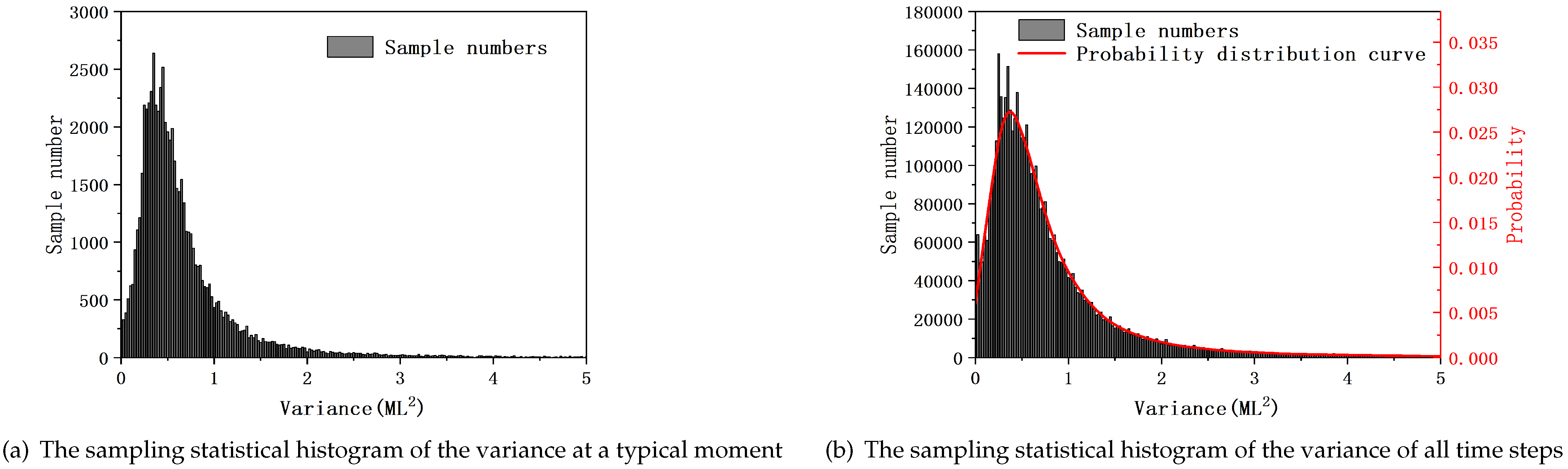
Then, the sampling statistical histogram of the variance at a typical moment and the sampling statistical histogram of the variance of all time steps are shown in Figure 7. The variance range is divided into 200 parts, and the corresponding sample numbers are given. This sampling statistical histogram of all time steps is quite similar to the sampling statistical histogram at a typical moment, which suggests that our previous assumption is reasonable. Then, a probability distribution curve is computed to fit the statistical histogram of all time steps. We note that the probability distribution curve in the figure is quite similar to the probability distribution curve of chi-square distribution, which suggests that the origin distribution of the lattice surface height data might be normal distribution. The probability distribution curve is then used as the variance probability function to simulate the stochastic oscillation of the surface sites. Combined with the RNN model, the prediction model of the kMC model is established and is called RNN.
4. Optimization Computation
The optimization goal is to achieve the desired average etching depth and average bottom roughness within the least amount of time. The RNN models and the probability function developed in the sections above are to predict the plasma state and the etch structure over t ∈ [t,t]. Long time horizon prediction is established by using the previous prediction results as the initial data for the current prediction. We note that the model error between the RNN models and the fluid model as well as the kMC model will accumulate over time and will lead to a huge prediction error at the final time. Thus, computing a single optimization problem from the beginning time step to the final time step will not be enough to compute the real optimization trajectories. Therefore, we apply a moving optimization method to compute the optimization trajectories, which limits the model error in one time step instead of the whole time horizon. In every time step t, an open-loop optimization problem is computed. The optimizing time range is from t to t and the optimized parameters are , , , . The initial condition is from the fluid model and the kMC model. The optimization problem is written below:
where , , and are the weight of the penalty on etching depth, bottom roughness and etching time, respectively; , , , and are the average etching depth at final time, the set average etching depth, the average bottom roughness at final time, and the set average bottom roughness, respectively; is the initial surface topology data (generated from the kMC model); , , , , , are the lowest and the highest bound of the optimized parameters. We note that the optimization problem can be solved in Matlab with the nonlinear programming (NLP) tool box. Specifically, we use the multistart function in Matlab and the solving algorithm is sequential quadratic programming (SQP). The multistart function is able to calculate multiple local solutions with several initial points and select the best solution as the global optimization solution. When the optimization problem is solved, the optimized parameters for the current time step will be stored and the optimization problem is resolved at the next time step. It should be noted that the optimization solution calculated at each time step would not be the real optimal solution due to model error. This error is limited in a single time step and is corrected in the next time step because the results of the fluid model and the kMC model are applied as the initial condition in the optimization problem. However, the global optimization solution is hard to obtain because the solutions at past time steps have already deviated from the global optimal trajectories.
5. Simulations and Results
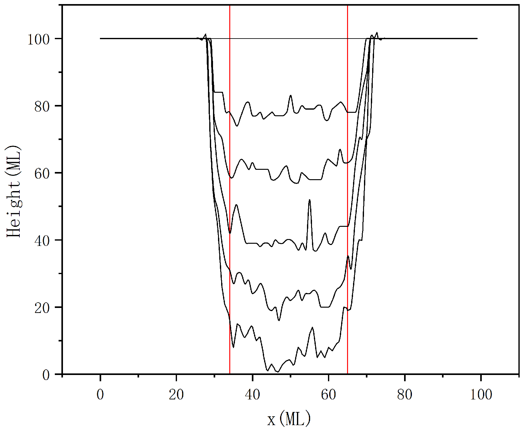
The plasma chemistry and microscopic structure of the etched lattice have been described in Section 2. The work pressure of the plasma chamber is set as 40 mTorr and the chamber temperature is set to be 60 °C. The ICP is excited by means of a ratio frequency (RF) power at 13.56 MHz supplied to the upper coils. Figure 8 shows an open-loop cross section profile evolution that was captured at 0 s, 3 s, 6 s, 9 s, 12 s, and 15 s. The etching depth is defined as the average etching depth (D) of all uncovered surface sites, and its unit is mL. Due to the existence of the resistive mask, the bottom surface is getting narrower over time. The red lines are used to define the range of the bottom surface in order to describe the bottom surface roughness more accurately. The bottom roughness () is defined by variance and its unit would be mL:
where N is the total number of the counted bottom surface sites, is the height of the surface site at position i, and is the average height of all counted bottom surface sites. In the following, we will present the results of the RNN models validation process and the optimization simulation results.
5.1. Validation of RNN Models
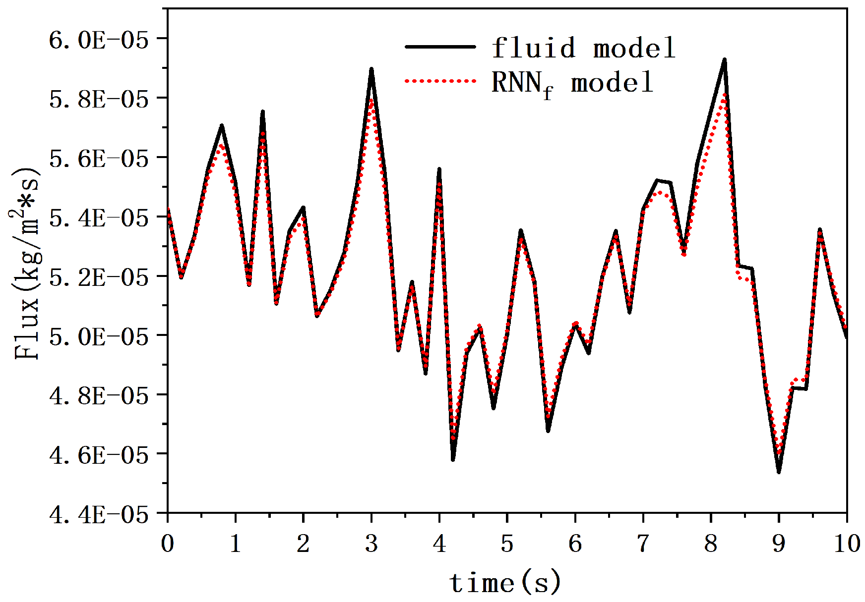
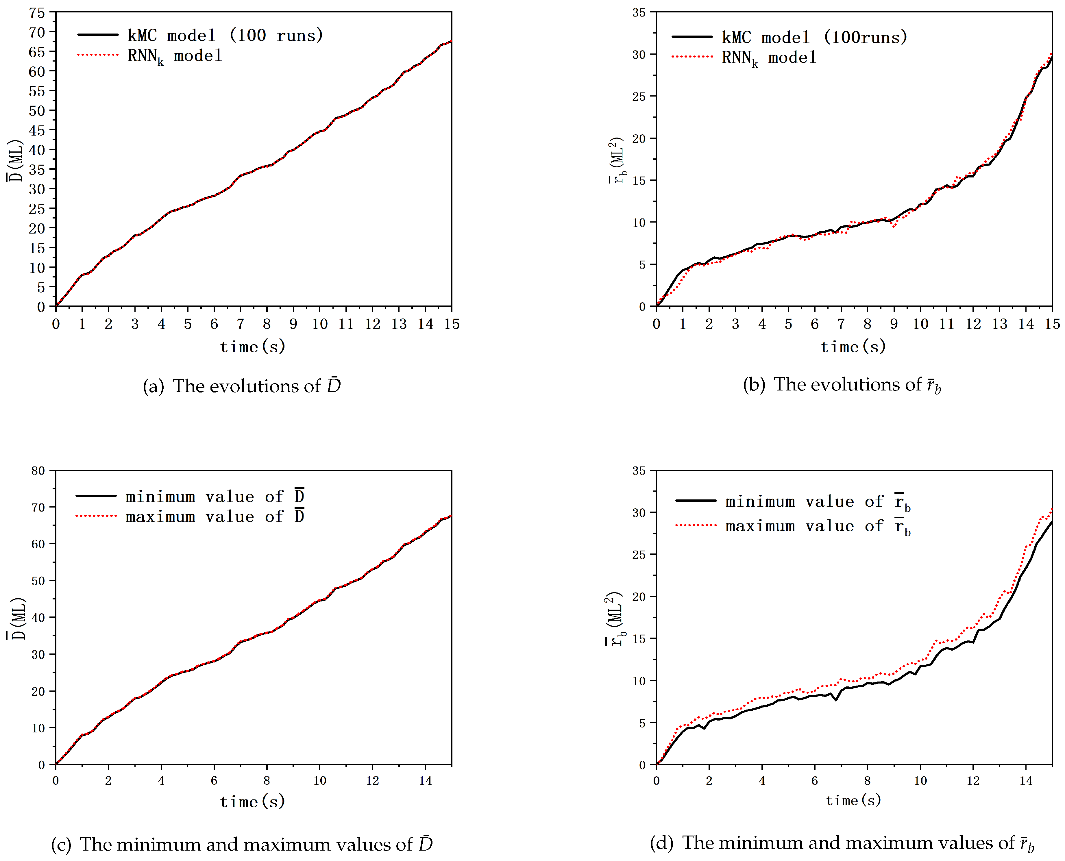
The prediction performance of the RNN models is carried out through the validation process. Figure 9 shows the Cl flux evolutions at location 1. The solid line represents the flux evolution of the fluid model, and the dotted line represents the predicted flux evolution of the RNN model. The flux data are sampled in every 0.2 s, and the model inputs are randomly selected from the selection range. Figure 10 shows the and evolutions and the minimum and maximum values of and among the 100 run kMC model simulations. In Figure 10a,b, the solid line represents and evolutions of the kMC model, and the dotted line represents the predicted and evolutions of the RNN model. In Figure 10c,d, the solid line represents the maximum values and the dotted line represents the minimum values. The and data are sampled in every 0.2 s, and the model inputs are randomly selected from the selection range. It should be noted that the evolutions of the kMC model are computed based on a 100 run simulations in order to obtain the expectation evolution. From (a) and (b), it can be seen that both the evolution trajectories of the RNN model and the RNN model are close to the trajectories of the fluid model and the kMC model, respectively. From (c) and (d), it can be seen that the average bottom roughness is strongly influenced by the stochastic nature of the etching process compared to the results of the average etching depth. From pre-experiments, the computation time of the fluid model and the kMC model in one time step (0.2 s) is about 20 min, while the computation time of the RNN model and the RNN model in one time step is only about 0.14 s. We note that the RNN models are sufficient to apply in the optimization process.
5.2. Optimization Simulations
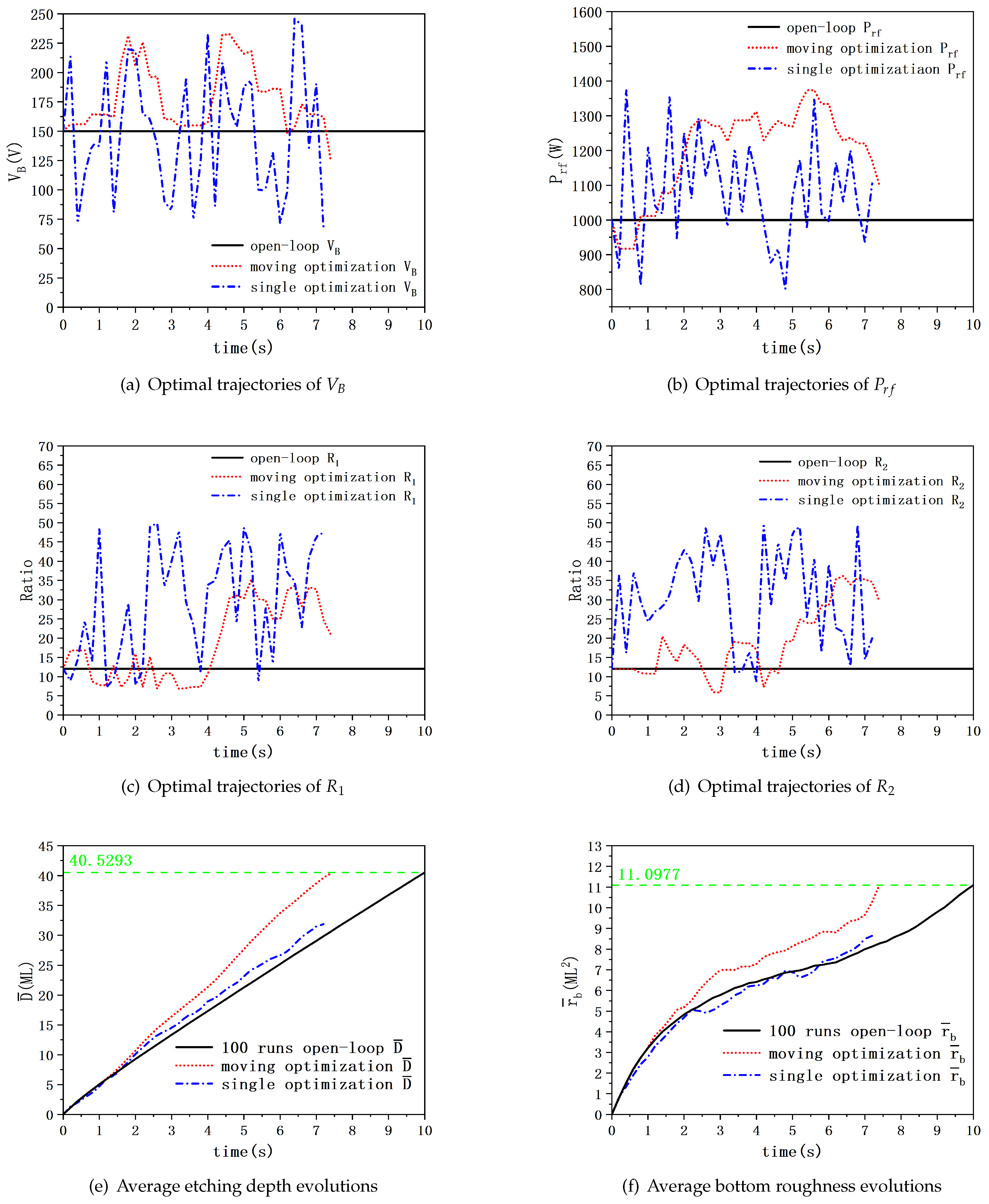
The optimization goal is to achieve the desired average etching depth and average bottom roughness within the least amount of time, and the optimized parameters would be , , , and . From the 100 run simulation, the final average etching depth and average bottom roughness after a 10 s etching process with , , W, V are 40.4293 ML and 11.0977 ML, which are chosen as and . Subsequently, we compute the moving optimization problem to calculate the optimal trajectories and the optimal total etching time. To emphasize the necessity of using the moving optimization method, we will also show the optimization results by solving a single optimization problem from the beginning time step to the final time step.
Figure 11 shows the optimal trajectories of , , , and the evolutions of and . Both results by using the moving optimization method and the single optimization method are shown. The average etching depth and average bottom roughness reach the desired level concurrently at 7.4 s by utilizing the moving optimization method, while the desired objects are not completed at the final time by utilizing the single optimization method. As we mentioned above, the model error will accumulate over time and the error would be so large that we cannot complete the desired objects by solving a single optimization problem. It should be noted that the optimized inputs would be largely modified in one time step when using the single optimization method, and this modification is feasible. Such techniques can be found in [37]. We also note that the optimization results by using the moving optimization problem will not be the global optimal solution due to the existence of the model error. Although the solutions might not be the best, using the moving optimization method can address the model error accumulation problem, and the desired average etching depth and bottom roughness are achieved in a shorter amount of time.
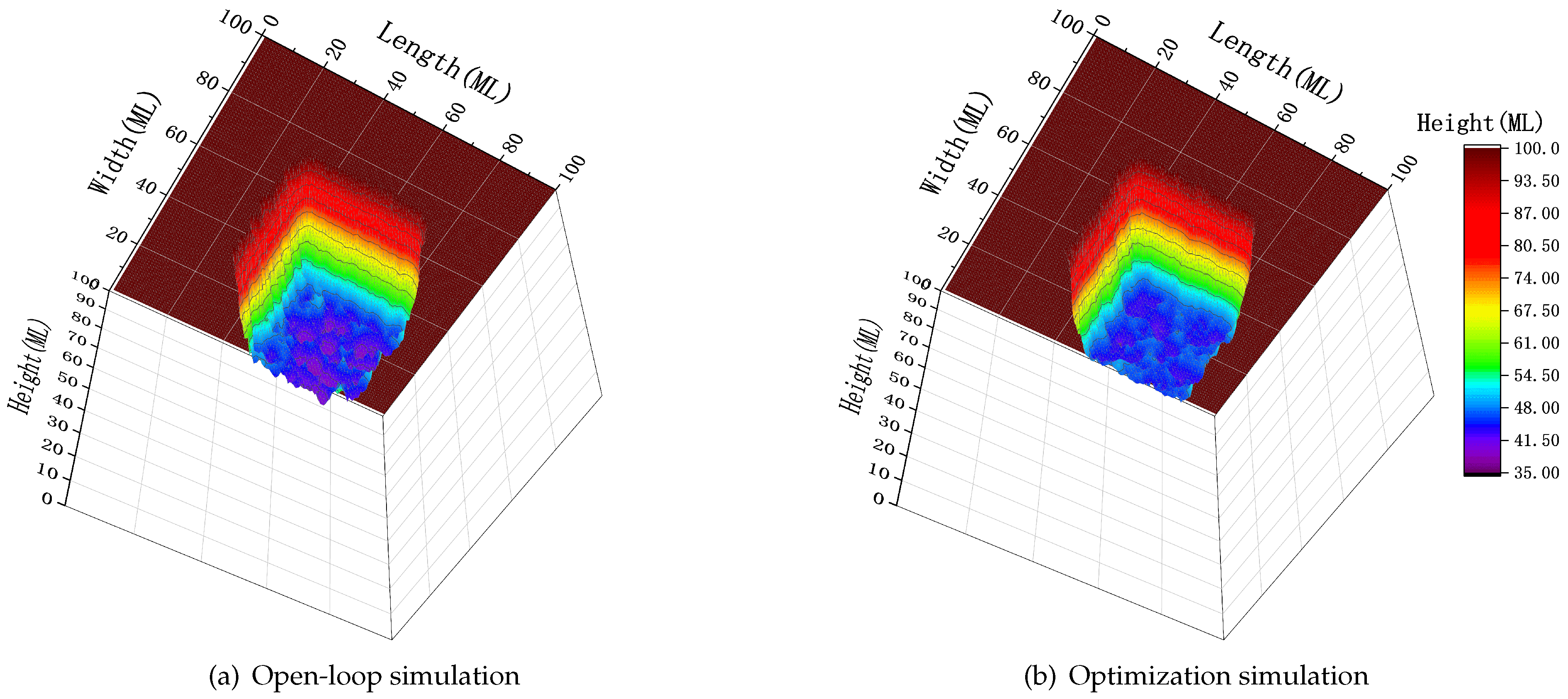
Figure 12 shows the three-dimensional profiles of the lattice at location 1 after a 10 s open-loop simulation and a 7.4 s optimization simulation (moving optimization method). The etching profiles are quite similar considering the natural stochastic characteristic of the etching process. The results show that our prediction model is accurate enough and the desired etching profile can be efficiently achieved in a shorter amount of time by utilizing the moving optimization method.
It should be noted that, although the microscopic processes of the real etch process are the same given a specific etch chemistry, the macroscopic dynamics and reaction kinetics of the plasma are highly equipment dependent with respect to the accuracy needed for real applications. While such high fidelity models are not openly available, equipment vendors typically have their own proprietary plasma models for their plasma processing equipments, and these models can be easily integrated into our multiscale modeling framework when needed.
6. Conclusions
In this work, a multiscale modeling and RNN based optimization framework of the plasma etch process on a three-dimensional substrate with uniform thickness using the inductive coupled plasma (ICP) was proposed. The macroscopic plasma model is simulated by a continuous fluid model and the microscopic etching process is simulated by a kMC model. A spatial-temporal discrete method is applied to compute these two models concurrently. Then, the RNN model and the RNN model are trained based on the open-loop simulation data of the fluid model and the kMC model, in order to reduce the computational complexity of these two models. The stochastic characteristic of kMC model is described by a probability function. Then, long time horizon prediction and optimization are calculated based on the RNN models and the probability function. A moving optimization method is applied to overcome the model error accumulation problem. The optimization goal is to achieve the desired average etching depth and bottom roughness within the least amount of time. In simulations and results, the validation experiments of RNN models are first implemented, and then the simulation results applying the optimized parameters are presented. The results demonstrate that our prediction model is accurate enough and the desired average etching depth and bottom roughness can be achieved in a shorter amount of time.
Author Contributions
Data curation: T.X. and D.N.; methodolog: T.X. and D.N.; software: T.X. and D.N.; supervision: D.N.; writing: T.X. and D.N. All authors have read and agreed to the published version of the manuscript.
Funding
This research was funded by the National Natural Science Foundation of China Grant No. U1609213.
Data Availability Statement
The data presented in this study are available on request from the corresponding author.
Conflicts of Interest
The authors declare no conflict of interest.
Abbreviations
The following abbreviations are used in this manuscript:
| MDPI | Multidisciplinary Digital Publishing Institute |
| DOAJ | Directory of Open Access Journals |
| TLA | Three Letter Acronym |
| LD | Linear Dichroism |
References
- Wu, B.; Kumar, A.; Pamarthy, S. High aspect ratio silicon etch: A review. J. Appl. Phys. 2010, 108, 051101. [Google Scholar] [CrossRef]
- Donnelly, V.; Kornblit, A. Plasma etching: Yesterday, today, and tomorrow. J. Vac. Sci. Technol. A Vacuum Surfaces Film. 2013, 31, 050825. [Google Scholar] [CrossRef] [Green Version]
- Mahorowala, A.P.; Sawin, H.H. Etching of polysilicon in inductively coupled Cl2 and HBr discharges. IV. Calculation of feature charging in profile evolution. J. Vac. Sci. Technol. B Microelectron. Nanometer Struct. Process. Meas. Phenom. 2002, 20, 1084–1095. [Google Scholar] [CrossRef]
- Aydil, E.; Quiniou, B.; Lee, J.; Gregus, J.; Gottscho, R. Incidence angle distributions of ions bombarding grounded surfaces in high density plasma reactors. Mater. Sci. Semicond. Process. 1998, 1, 75–82. [Google Scholar] [CrossRef]
- Sethian, J.A.; Adalsteinsson, D. An overview of level set methods for etching, deposition, and lithography development. IEEE Trans. Semicond. Manuf. 1997, 10, 167–184. [Google Scholar] [CrossRef] [Green Version]
- Sethian, J. Evolution, Implementation, and Application of Level Set and Fast Marching Methods for Advancing Fronts. J. Comput. Phys. 2001, 169, 503–555. [Google Scholar] [CrossRef] [Green Version]
- Chatterjee, A.; Vlachos, D. An overview of spatial microscopic and accelerated kinetic Monte Carlo methods. J. Comput-Aided Mater. 2007, 14, 253–308. [Google Scholar] [CrossRef]
- Gosalvez, M.; Xing, Y.; Sato, K.; Nieminen, R. Atomistic methods for the simulation of evolving surfaces. J. Micromech. Microeng. 2008, 18, 055029. [Google Scholar] [CrossRef]
- Guo, W.; Sawin, H. Review of profile and roughening simulation in microelectronics plasma etching. J. Phys. D Appl. Phys. 2009, 42, 194014. [Google Scholar] [CrossRef]
- Petsev, N.D.; Leal, L.G.; Shell, M.S. Coupling discrete and continuum concentration particle models for multiscale and hybrid molecular-continuum simulations. J. Chem. Phys. 2017, 147, 234112. [Google Scholar] [CrossRef]
- Xiao, S.; Belytschko, T. A bridging domain method for coupling continua with molecular dynamics. Comput. Methods Appl. Mech. Eng. 2004, 193, 1645–1669. [Google Scholar] [CrossRef]
- Varshney, A.; Armaou, A. Multiscale optimization using hybrid PDE/kMC process systems with application to thin film growth. Chem. Eng. Sci. 2005, 60, 6780–6794. [Google Scholar] [CrossRef]
- He, C.; Ge, J.; Qi, D.; Gao, J.; Chen, Y.; Liang, J.; Fang, D. A multiscale elasto-plastic damage model for the nonlinear behavior of 3D braided composites. Compos. Sci. Technol. 2019, 171, 21–33. [Google Scholar] [CrossRef]
- Rodrigues, E.A.; Manzoli, O.L.; Bitencourt, L.A. 3D concurrent multiscale model for crack propagation in concrete. Comput. Methods Appl. Mech. Eng. 2020, 361, 112813. [Google Scholar] [CrossRef]
- Crose, M.; Kwon, J.S.I.; Tran, A.; Christofides, P.D. Multiscale modeling and run-to-run control of PECVD of thin film solar cells. Renew. Energy 2017, 100, 129–140. [Google Scholar] [CrossRef] [Green Version]
- Xiao, T.; Ni, D. Multiscale modeling and neural network model based control of a plasma etch process. Chem. Eng. Res. Des. 2020, 164, 113–124. [Google Scholar] [CrossRef]
- Ning, H.; Jing, X. Identification of partially known nonlinear stochastic spatio-temporal dynamical systems by using a novel partially linear Kernel method. IET Control Theory Appl. 2015, 9, 21–33. [Google Scholar] [CrossRef]
- Charles, P.; Raja, S.; Sura, N.; Mulla, S. System identification based aeroelastic modeling for wing flutter. Aircr. Eng. Aerosp. Technol. 2018, 90, 261–269. [Google Scholar]
- Narendra, K.S.; Parthasarathy, K. Identification and control of dynamical systems using neural networks. IEEE Trans. Neural Netw. 1990, 1, 4–27. [Google Scholar] [CrossRef] [Green Version]
- Aguilar, C.Z.; Aguilar, J.G.; Martinez, V.A.; Ugalde, H.R. Fractional order neural networks for system identification. Chaos Solitons Fractals 2020, 130, 109444. [Google Scholar] [CrossRef]
- Hopfield, J. Neural Networks and Physical Systems with Emergent Collective Computational Abilities. Proc. Ntal. Acad. Sci. USA 2018, 79, 7–19. [Google Scholar]
- Hochreiter, S.; Schmidhuber, J. Long Short-Term Memory. Neural Comput. 1997, 9, 1735–1780. [Google Scholar] [CrossRef] [PubMed]
- Cho, K.; van Merriënboer, B.; Gulcehre, C.; Bahdanau, D.; Bougares, F.; Schwenk, H.; Bengio, Y. Learning Phrase Representations using RNN Encoder–Decoder for Statistical Machine Translation. In Proceedings of the 2014 Conference on Empirical Methods in Natural Language Processing (EMNLP), Doha, Qatar, 25–29 October 2014; pp. 1724–1734. [Google Scholar]
- Lukoševičius, M.; Jaeger, H. Reservoir computing approaches to recurrent neural network training. Comput. Sci. Rev. 2009, 3, 127–149. [Google Scholar] [CrossRef]
- Funahashi, K.; Nakamura, Y. Approximation of dynamical systems by continuous time recurrent neural networks. Neural Netw. 1993, 6, 801–806. [Google Scholar] [CrossRef]
- Jaeger, H.; Haas, H. Harnessing Nonlinearity: Predicting Chaotic Systems and Saving Energy in Wireless Communication. Science 2004, 304, 78–80. [Google Scholar] [CrossRef] [PubMed] [Green Version]
- Trischler, A.P.; D’Eleuterio, G.M. Synthesis of recurrent neural networks for dynamical system simulation. Neural Netw. 2016, 80, 67–78. [Google Scholar] [CrossRef] [PubMed] [Green Version]
- Pitchford, L. LXCat: A web-based, community-wide project on data for modeling low temperature plasmas. Bull. Am. Phys. Soc. 2014, 59, AM2-005. [Google Scholar]
- Stockholm, S. GEC ICP Reactor, Argon Chemistry. 2018, pp. 22–23. Available online: https://www.comsol.com/ (accessed on 14 January 2021).
- Chanson, R.; Rhallabi, A.; Fernandez, M.; Cardinaud, C.; Bouchoule, S.; Gatilova, L.; Talneau, A. Global Model of Cl2/Ar High-Density Plasma Discharge and 2D Monte-Carlo Etching Model of InP. IEEE Trans. Plasma Sci. 2012, 40, 959–971. [Google Scholar] [CrossRef]
- Tinck, S.; Boullart, W.; Bogaerts, A. Investigation of etching and deposition processes on Cl2/O2/Ar inductively coupled plasmas on silicon by means of plasma surface simulations and experiments. J. Phys. D Appl. Phys. 2009, 42, 095204. [Google Scholar] [CrossRef]
- Osano, Y.; Ono, K. An Atomic Scale Model of Multilayer Surface Reactions and the Feature Profile Evolution during Plasma Etching. Jpn. J. Appl. Phys. 2005, 44, 8650. [Google Scholar] [CrossRef]
- Osano, Y.; Mori, M.; Itabashi, N.; Takahashi, K.; Eriguchi, K.; Ono, K. A Model Analysis of Feature Profile Evolution and Microscopic Uniformity during Polysilicon Gate Etching in Cl2/O2 Plasmas. Jpn. J. Appl. Phys. 2006, 45, 8157–8162. [Google Scholar] [CrossRef]
- Agarwal, A.; Kushner, M. Plasma atomic layer etching using conventional plasma equipment. J. Vac. Sci. Technol. A Vacuum Surfaces Film. 2009, 27, 37–50. [Google Scholar] [CrossRef]
- Chiaramonte, L.; Colombo, R.; Fazio, G.; Garozzo, G.; Magna, A.L. A numerical method for the efficient atomistic simulation of the plasma-etch of nano-patterned structures. Comput. Mater. Sci. 2012, 54, 227–235. [Google Scholar] [CrossRef]
- Chang, J.P.; Sawin, H.H. Kinetic study of low energy ion-enhanced polysilicon etching using Cl, Cl2, and Cl+ beam scattering. J. Vac. Sci. Technol. A 1997, 15, 610–615. [Google Scholar] [CrossRef]
- Kanarik, K.J.; Lill, T.; Hudson, E.A.; Sriraman, S.; Tan, S.; Marks, J.; Vahedi, V.; Gottscho, R.A. Overview of atomic layer etching in the semiconductor industry. J. Vac. Sci. Technol. A 2015, 33, 020802. [Google Scholar] [CrossRef] [Green Version]
Figure 1.
The half cross section of the ICP equipment and the spatial discrete method are shown. A computational result of electron density after 1 s is also shown.
Figure 1.
The half cross section of the ICP equipment and the spatial discrete method are shown. A computational result of electron density after 1 s is also shown.

Figure 2.
The simulation box is shown. The black sphere is the particle coming from plasma, which is above the vacuum region and not shown in simulation. Each cubic cell contains only one atom, and the lattice is formed by these cells.
Figure 2.
The simulation box is shown. The black sphere is the particle coming from plasma, which is above the vacuum region and not shown in simulation. Each cubic cell contains only one atom, and the lattice is formed by these cells.

Figure 3.
The flowchart of the simulation numerical algorithm is shown. All sub-events in the flowchart are already discussed.
Figure 3.
The flowchart of the simulation numerical algorithm is shown. All sub-events in the flowchart are already discussed.

Figure 4.
The RNN and its unfold structure are shown, where W is the RNN parameters, h is the hidden state, x is the model inputs, and o is the model outputs.
Figure 4.
The RNN and its unfold structure are shown, where W is the RNN parameters, h is the hidden state, x is the model inputs, and o is the model outputs.

Figure 5.
The training process of the sub models and the RNN model. The validation data are not used for training the sub models.
Figure 5.
The training process of the sub models and the RNN model. The validation data are not used for training the sub models.

Figure 6.
The statistical properties of the variance is shown.

Figure 7.
The sampling statistical histogram of the variance at a typical moment and the sampling statistical histogram of the variance of all time steps are shown. A probability distribution curve is computed to fit the statistical histogram of all time steps.
Figure 7.
The sampling statistical histogram of the variance at a typical moment and the sampling statistical histogram of the variance of all time steps are shown. A probability distribution curve is computed to fit the statistical histogram of all time steps.

Figure 8.
The open-loop cross section profile evolution that was captured at 0 s, 3 s, 6 s, 9 s, 12 s, and 15 s.
Figure 8.
The open-loop cross section profile evolution that was captured at 0 s, 3 s, 6 s, 9 s, 12 s, and 15 s.

Figure 9.
The evolutions of the Cl flux at location 1. The solid line represents the flux evolution of the fluid model, and the dotted line represents the predicted flux evolution of the RNN model.
Figure 9.
The evolutions of the Cl flux at location 1. The solid line represents the flux evolution of the fluid model, and the dotted line represents the predicted flux evolution of the RNN model.

Figure 10.
The evolutions of and are shown in (a,b). The minimum and maximum values of and among the 100 runs kMC model simulations are shown in (c,d).
Figure 10.
The evolutions of and are shown in (a,b). The minimum and maximum values of and among the 100 runs kMC model simulations are shown in (c,d).

Figure 11.
The optimal trajectories of , , , and the evolutions of and . Both the results of the moving optimization method and single optimization method are shown.
Figure 11.
The optimal trajectories of , , , and the evolutions of and . Both the results of the moving optimization method and single optimization method are shown.

Figure 12.
The three-dimensional profiles of the lattice at location 1 after a 10 s open-loop simulation and a 7.4 s optimization simulation.
Figure 12.
The three-dimensional profiles of the lattice at location 1 after a 10 s open-loop simulation and a 7.4 s optimization simulation.

Publisher’s Note: MDPI stays neutral with regard to jurisdictional claims in published maps and institutional affiliations. |
© 2021 by the authors. Licensee MDPI, Basel, Switzerland. This article is an open access article distributed under the terms and conditions of the Creative Commons Attribution (CC BY) license (http://creativecommons.org/licenses/by/4.0/).
Share and Cite
MDPI and ACS Style
Xiao, T.; Ni, D. Multiscale Modeling and Recurrent Neural Network Based Optimization of a Plasma Etch Process. Processes 2021, 9, 151. https://0-doi-org.brum.beds.ac.uk/10.3390/pr9010151
AMA Style
Xiao T, Ni D. Multiscale Modeling and Recurrent Neural Network Based Optimization of a Plasma Etch Process. Processes. 2021; 9(1):151. https://0-doi-org.brum.beds.ac.uk/10.3390/pr9010151
Chicago/Turabian StyleXiao, Tianqi, and Dong Ni. 2021. "Multiscale Modeling and Recurrent Neural Network Based Optimization of a Plasma Etch Process" Processes 9, no. 1: 151. https://0-doi-org.brum.beds.ac.uk/10.3390/pr9010151
Note that from the first issue of 2016, this journal uses article numbers instead of page numbers. See further details here.