Ontology-Based Process Modelling-with Examples of Physical Topologies

Abstract

Reductionism and splitting application domain into disciplines and identify the smallest required model-granules, termed ”basic entity” combined with systematic construction of the behaviour equations for the basic entities, yields a systematic approach to process modelling. We do not aim toward a single modelling domain, but we enable to address specific application domains and object inheritance. We start with reductionism and demonstrate how the basic entities are depending on the targeted application domain. We use directed graphs to capture process models, and we introduce a new concept, which we call ”tokens” that enables us to extend the context beyond physical systems. The network representation is hierarchical so as to capture complex systems. The interacting basic entities are defined in the leave nodes of the hierarchy, making the overall model the interacting networks in the leave nodes. Multi-disciplinary and multi-scale models result in a network of networks. We identify two distinct network communication ports, namely ports that exchange tokens and ports that transfer information of tokens in accumulators. An ontology captures the structural elements and the applicable rules and defines the syntax to establish the behaviour equations. Linking the behaviours to the basic entities defines the alphabet of a graphical language. We use this graphical language to represent processes, which has proven to be efficient and valuable. A set of three examples demonstrates the power of the graphical language. The Process Modelling framework (ProMo) implements the ontology-centred approach to process modelling and uses the graphical language to construct process models.

1. Introduction

The title refers to modelling, implying the generation of what is often referred to as a digital twin, namely, a digital reproduction of a process’ behaviour. The term “model” is used in very different contexts and, correspondingly, has many facets. However, people always model processes for a specific purpose, and most often, the main objective is to generate a simulation with given inputs and a specified process characteristic. Many applications use simulation as an inner loop, with the outer loop defining the main objective, such as optimisation. For example, process design seeks optimal process parameters and optimising control finds an input that optimises an objective. From this perspective, modelling naturally sits at the very front end of the overall process, associated with solving a simulation-related problem, which makes modelling a core activity; therefore, errors in the model are the most costly ones. Thus, it is a natural request to have a systematic approach to modelling that is safe in terms of generating structurally sound models.

We claim that chemical engineering lacks such a systematic model-building process. The closest we have is flowsheeting software which uses customised unit-operation building blocks as its base entities. Readers interested in the historical aspects are referred to [1]. These traditional modelling environments suffer from a couple of problems, which provides the motivation for seeking an alternative, new approach. Let us give a couple of observation-based reasons.

1.1. Why We Need a Systematic Modelling Approach

Incompleteness: Published models tend to be incomplete, in the sense that, usually, the authors do not provide all relevant information leading to the given input/output behaviour. As an example, the publication [2] describes a non-trivial decanting two-liquid-phase reactor. On page two is a simple figure that shows the process schematically. On page three, one finds the mathematical model, which consists of eleven equations. It is left to the knowledgable reader to interpret these equations and determine which one describes which element in the process. If the exercise is used to analyse these equations, close to one hundred equations are obtained, which explain the nature of the description and assumptions in detail. The number of equations is somewhat puzzling, considering the low structural complexity, and a strong indication that the modeller hid many details or is not aware of them. The model is not particularly complex. It describes the reactor’s contents as two lumped systems, each with component balances for five species, an energy balance for the two lumps together and a description of the reactor’s holdup.

Flowsheeting-balance closure: Above, we mentioned flowsheeting. The typical supplier provides libraries, often designed for particular users, and thus subdiscipline-specific process units or component models. A model builder or composer then utilises the library to construct process models. Next, a solver kernel is attached, providing the implementation of the appropriate solution methods. Examples are gPROMS^®, ASPEN^® and UNISYM^®. Within parts of the user community, it seems to be well known that these simulators do not guarantee the conserved quantities’ closure, which represents a fundamental problem for most applications.

Documentation: Process-unit-oriented libraries document the unit’s behaviour on the unit level. The details of the models are, therefore, mostly hidden. There is little detail on the actual implementation, as it is considered unnecessary information for the typical user. This information is seen as only relevant for the expert implementing the software module. The result of this is that the individual models are black boxes that provide input/output behaviour. Consequently, the software users must work on the corresponding level of insight; they do not have access to the lower modelling level, through either the code or the documentation.

1.2. An Alternative

The author’s process modelling project ProMo takes an alternative route. While we also build the models using a set of building blocks, our basic model entities are below the unit-operation level. They are in the context of the model application on the smallest granularity level; we call them ”basic entities”. It is essential to acknowledge that these entity blocks are basic on a particular granularity level, with the granularity level depending on the intended application.

While macroscopic physics was the starting point, the concept has been expanded to other disciplines, including control and lower-scale physics, like molecular dynamics. The project constructs its building blocks only from the fundamental concepts defining discipline-basic entities. These entities form the foundation for the discipline-mechanistic construction of the models. The underlying philosophy is therefore reductionism. Since they are deductive, mechanistic models cannot necessarily adequately capture real-world behaviours; a practical modelling system must allow for both glass-box (white-box) models and holistic surrogates (black-box models).

State-space representation: The approach is state-space based. For macroscopic physical systems, the conserved quantities serve as the state. Consequently, any numerical method, primarily integration, closes the respective balance to the defined accuracy. We can thus always guarantee the closure of the fundamental quantities once the algorithm has converged.

Implementation: The definition space, namely, the part associated with defining the basic building blocks, is ontology-driven. Using ontologies at the front end of the definition process imposes a structure onto the process and yields overall consistency. On a more technical level, the equations are in the ”pure” form, meaning neither the user nor the software performs any transformations or substitutions. Each equation appears only once in the code, in contrast to unit-operation-based modelling, where each module typically represents the complete model for the mimicked unit. All model-related code is centralised and appears only once. Any composite model uses indexing to refer to the block representations, which renders modelling a bookkeeping problem.

Project Process Modelling ProMo’s main objective: The project, which we named ProMo, aims to construct an environment that steers the modelling process as tightly as possible, without imposing constraints, which we achieve by using an ontology. The domain-specific ontology defines the structure of the information underlying the models which will be constructed in the domain captured by the ontology. The construction of the ontology is thus essential for the project’s software. The following section is devoted to defining the elements of the ontology.

This paper: The goal of the paper is to define the basis for the graphical representation of process models. In the first step, we discuss the reductionism-based approach, seeking a minimal set of entities that enable us to construct the models for a class of modelling domains. Next, we discuss an abstraction that allows us to extend the modelling beyond physical systems. An ontology tailored to specific application domains provides the fundamental structures for the behaviour description and represents the construction codes for complex models. Defining the entity behaviour in terms of mathematical equations, namely as input/output functions, and linking them to the graphical objects sets the stage for the graphical representation. The latter forms the basis of a graphical language, which we demonstrate the use of in a set of applications. The visual language is handy when discussing a paper-and-pencil model design, and it is also directly used in the ProMo model design tool.

We will leave out two main parts from ProMo. The first is the definition of the behaviour equations, which we will have to present on another occasion. The core is the definition of a formal language and the ability to compile it into different target codes [3]. The second is the generation of the actual simulation code, which is similarly technical in terms of computer science issues, including the realisation of the automatic generation of application interfaces and the semantic network for interoperability. Both sections are full of technical details, which are not relevant to the current exposition.

2. Reductionism

The objective is to generate a mathematical representation of the modelled system, confining the description to a mathematical input/output representation. This behaviour description will be the result of a network of interacting basic entities. For these reasons, we apply reductionism to identify the smallest underlying relevant entities in the context of an intended application. Applying reductionism in model construction places the base entities’ definition, the base building blocks, into the centre of development.

From the perspective of mathematics, describing the dynamic results in time-dependent differential equations for time-discrete systems uses time-difference equations, and for event-discrete systems, automata are used, and thus state-discrete difference equations. All the models must satisfy a fundamental condition: Independent of their nature, all equations must represent realisable systems, which, for physics, translates to causal or nonanticipative systems.

2.1. Continuous Macroscopic Physical Systems

Reductionism, when applied to continuous macroscopic systems, recursively splits the physical system into smaller volumes. The dividing process stops once one reaches a “suitable” granularity. The resulting base entities are three-dimensional dynamical systems that live in four-dimensional spacetime. Partial differential equations describe their behaviour and the applicable fundamental conservation principles. They describe the evolution of the state of the modelled smallest volume; the identified entity, namely, the state change is the consequence of the interaction with the environment. As a mechanism to establish the conservation and balance equations, one “walks” the surface of the volume and accounts for all interactions, and thus the conserved quantity crossing the boundary, which gives rise to the term “control volume”. Overall, an accounting operation, that is based on the system and the conserved quantity. The assembly of extensive quantities then represents the fundamental state of the volume. The network of elementary control volumes, the base entities, and their interactions across common boundaries describe the behaviour of a modelled fundamental entity.

2.2. Particulate Physical Systems

In many cases, the modelling is not focused on a complexity described by a hierarchy of systems, but complexity arises from having many objects on the same level of granularity. Examples include molecular dynamics or large quantities of particles or models that approximate continuous systems with many particles, such as smoothed-particle hydrodynamics [4] or the like. One of the main problems with these systems is the formulation of boundary conditions and the forces acting between them. The fundamental entity in such systems is the particle.

Dynamic state equations describe the behaviour of the particles. With the particles’ capacities, this results in ordinary differential equations, with population balances being a typical representation. As each particle has a state, the size of the equation set is an apparent computational problem.

2.3. Control Systems

Control is an enabling technology. It allows for steering and maintaining the state of the process. Processes must be driven; there must be driving forces acting on the process to keep it from its natural steady state. Thus, processes must be embedded in an environment that is not in equilibrium with the process. The parts that make up the environment are also not in equilibrium with each other, thereby enabling the process to “run” like a water wheel between an elevated water reservoir, ejecting it to the lower-level reservoir. This Carnot-kind of viewpoint is very generic.

The manipulation of the flows between the different constituent parts of the system makes it possible to move the process into any place in the attainable region defined by the environment (Refers to controllability.). Thus, the state of the environment determines the attainable region, and it is the main controls that act on the flows between the environment and the system that control the overall state of the process.

A control system implements the externally provided objectives in terms of target values for states or state-dependent quantities. Analysing the ideal controller, namely, requesting that the process instantaneously follows the given setpoint, shows that the controller would have to invert the plant. Since the plant exhibits capacity behaviour, the inversion is not causal, and therefore not feasible. Consequently, all controllers implement an approximate inverse plant, and their states mirror the plant’s states.

The nature of the equations depends on the nature of the controlled system. In the case of a sampled system, time-discrete difference equations are used, while for event-observed systems, an automaton is used, and thus also a difference equation. Continuous control implies analogue controllers, which are physical systems and may also be modelled in the physical domain.

2.4. Other Relevant Subjects

The simulation of technical and natural systems is often augmented with analytical tools. For technical systems, these may be techno-economical or ecological analytical tools, such as Life-Cycle Analysis or financial return. Statistical tools also belong to this class of extension.

3. Networks & Tokens

Overall, reductionism describes the modelled physical system as a network of interacting capacities that partially project onto the control, and all other relevant subjects or disciplines.

If we attach the term ”discipline” to physics and control, it is natural to subdivide each discipline into more specific ”subdisciplines”. For physics, this leads to a ”tree” of disciplines, which captures continuous, macroscopic, particulate, small-scale, atomic, etc. For control, the control pyramid is used, with the event-discrete layers on top, planning, scheduling, optimisation and sampled systems below, as well as model-predictive control, optimising control, unit-level control and low-level control.

The subdivision into disciplines and subdisciplines for physics is somewhat involved. Carrying out subdivision on a global level leads to a very complex and large framework. The members of the European Material Modelling Council are working on such a global classification, called the European Materials Modelling Ontology (EMMO) (For information, see https://emmc.info/emmo-info/, accessed on 27 March 2021 and for the ontology https://github.com/emmo-repo/EMMO, accessed on 27 March 2021). ProMo enables the definition of subtrees of the EMMO discipline classification, aiming at the construction of smaller EMMO-related ontologies, which are more focused on specific application domains. Also, ProMo aims to handle large-scale models and is not limited to materials, although it has a substantial section that is associated with materials.

3.1. Higher-Level Abstraction

3.1.1. Tokens

The multidisciplinary nature of the problem requires higher-level abstraction. The network is the first element which we lift by adding the concept ”tokens”. The domain-specific ”tokens” are the items living in the specific ”networks”. The ”networks”, have directed graphs as node capacities for the ”tokens”, whilst the edges are transporting ”tokens”. The ”tokens” within a capacity, a graph’s node, define the state of the node.

For physical systems, we use the conserved quantities as ”tokens”, primarily mass, energy and momenta, but also items that make up a population. In control, the token is a signal, and a monetary measure in economic systems. Thus, the abstraction of a (sub)-discipline is a network of capacities for tokens communicating tokens.

3.1.2. Intra-Faces and Inter-Faces

The definition of networks and tokens provides the basis for the definition of the two types of interaction: ”Intraface” is a communication path for tokens, while ”interface” communicates state-dependent information.

The ”intraface” thus couples similar networks, where similar implies that the two coupled ”networks” contain the same ”tokens”. An ”intraface” thus communicates ”tokens”. In contrast, if one couples two networks that are not similar, but have different ”tokens”, the link will transfer information, usually state-related information. To give an example, in the first case, one may transfer mass from a liquid to a gas phase. Mass is transferred through an ”intraface”. In contrast, for the second case, state information is passed to the controller through an ”interface”. The generated value for a manipulated variable in the physical system is the information given back to the physical system.

3.1.3. Nodes & Arcs

”Networks” are directed graphs. The ”nodes” or vertices represent the capacities for the tokens, and the ”arcs” or edges represent the flow of tokens. The directed arcs define a reference coordinate for each flow of tokens. Tokens of the same type may be grouped and transported by one arc.

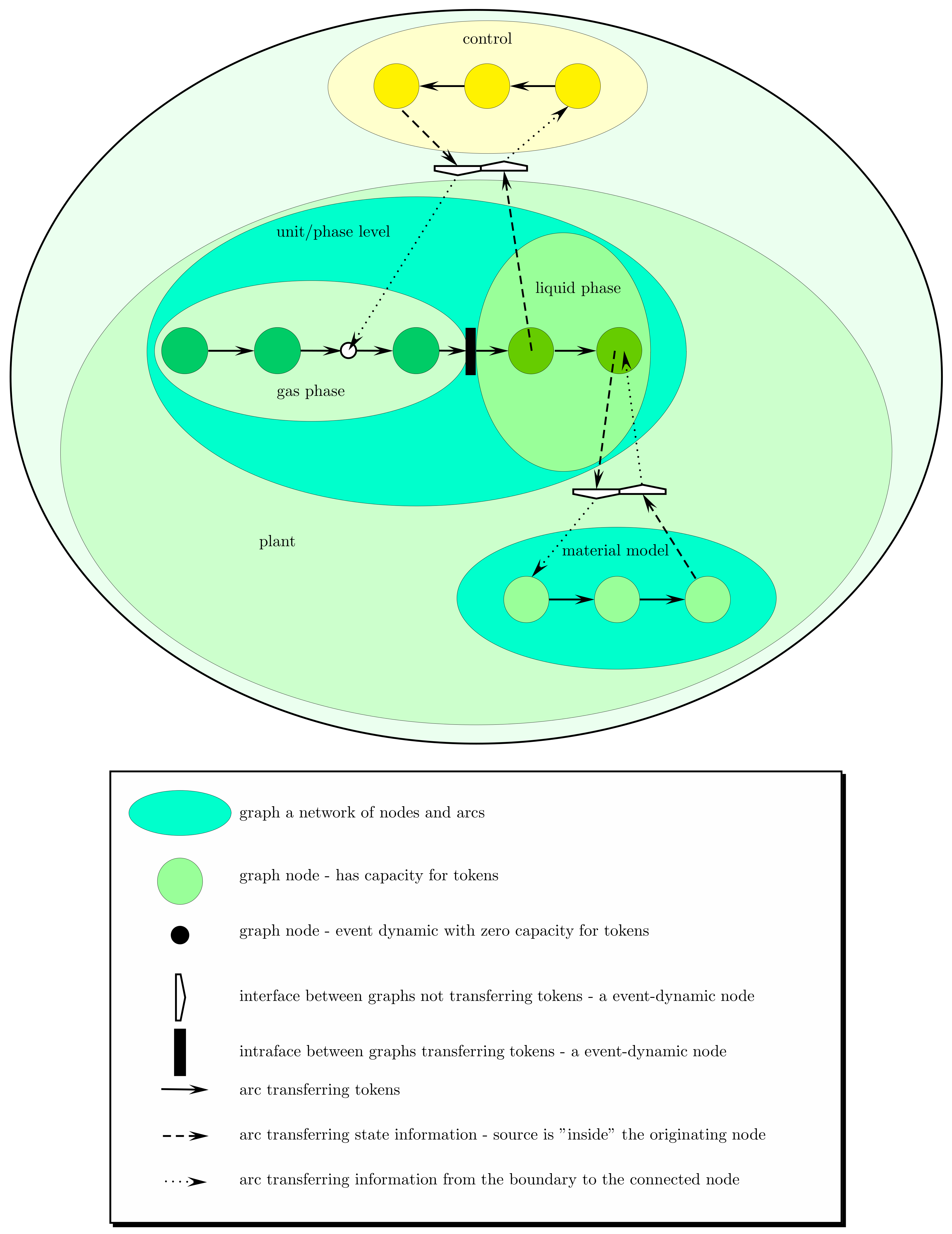
Figure 1 shows all elements that make up the graph of graphs in a minimal example. The physical part of the plant, labelled with ”plant”, shows two networks, a liquid phase and a gas phase. Those two communicate with each other mass through a common ”intraface”. The liquid phase seeks material information from the material model, providing state information, typically species, pressure, temperature, and asking for a physical property, like density. Both channels operate through an ”interface”. The liquid phase also provides state information to a control network, again through ”interfaces”.

On the smallest scale, the ”nodes” also represent basic entities, which result from applying reductionism.

3.2. Formal Definitions—A Summary

The discussion in this section yields the definition of a couple of items:

Network:

“directed graph” representing the structured modelled system on a given granularity level.

Token:

“item” living in the “network”.

Node:

is a component of the “network”, which exhibits the ability to store “tokens”.

Arc:

is the component of the “network” representing the transfer of “tokens” between “nodes”.

Basic or fundamental entity:

is the smallest building block required to establish models in a given domain – the smallest basic item in a hierarchical granular system (European Committee for Committee for Standardisation CEN defines the term entity in the Workshop agreement MODA [5]). In other words, a basic entity is context-dependent and defined as the smallest granule that describes the group of composite systems. It is the application of the resulting model that determines the granule resolution.

Intraface:

communicates bidirectionaly tokens between nodes of two intra-related networks.

Interface:

communicates unidirectionally state-related information from a node of one network to a node in the inter-related network.

4. Basic Entities

“Entities” are discipline and application-specific, but also have some common properties, namely, the dependency on the free variables’ time and the three spatial variables, and thus the four-dimensional spacetime.

4.1. Time Aspects

Any model of a dynamic system embraces three time scales: (i) “constant”—the parts that are not changing with time, (ii) “dynamic”—those parts that exhibit dynamic capacity behaviour, and (iii) “event-dynamic”—those parts that change instantaneously.

4.2. Spatial Aspects

For “physical entities”, objects live in the four-dimensional spacetime. Continuous domains may then be categorised into classes.

Lumped systems:

are finite-dimensional volumes where the relevant intensive properties are not a function of the spatial coordinates, thus a spatial domain in which the relevant intensive properties are uniform in terms of the spatial distribution.

In contrast:

Distributed systems:

are finite-dimensional volumes where the relevant intensive properties are a function of the spatial coordinates, thus a spatial domain in which the relevant intensive properties are not uniform in terms of the spatial distribution.

Both “lumped systems” and “distributed systems” are basic building blocks (entities) when modelling macroscopic systems.

4.3. Deterministic, Stochastic & Ergodic

“Entities” may exhibit deterministic or stochastic behaviour. Given a deterministic input and a fixed entity, then the output is also deterministic. If any either the input or the entity’s properties are stochastic, then the output will also be stochastic.

“Egodicity” is when the time average is identical to the state average of identical processes at one point in time, or in other terms: “all accessible microstates are “equiprobable” over a long period of “time” (Source wikipedia).

4.4. Continuous Physical Systems

The nature of “basic entities” is described above. The objective is to generate equations for numerical computations. Therefore, we need to define the input/output behaviour as a set of mathematical equations.

We create the equations on the background of system theory [6], leaning towards Willhelm’s behaviour theory [7]. A state-space view serves the purpose of analysing and controlling the structure. The “state” takes a centre position. The definition of the term “state” is hard to trace, but one can find an early version in Caratheodory [8]: “ ... ein “Zustand” des Systems S, und wir wollen für die Zahlen $x_i$ selbst den Namen “Zustandskoordinaten” einführen. ” We shall have a look at the two essential domains, namely, continuous systems and control.

4.4.1. Thermodynamic Systems

The domain of macroscopic, thermodynamic systems builds on the concepts of conserved mass, energy and momentum, while Newton’s laws govern mechanical systems. Focusing on thermodynamic systems, one would typically also allow for the conversion of chemical or biological species, which, building on atomic mass conservation, gives rise to species balances.

Balances and conservations follow the same principle: one defines them by walking the system’s boundary, accounting for all the quantities crossing the surface. The change occurring inside the system is then equated with the transfer, and, in the case of species conversion, it is augmented with the species’ transposition, yielding a “species balance”. Expressing these concepts verbally: “accumulation = net flow across the surface + net consumption”. Conservation principles do not include the last term; it only appears as a consequence of allowing for conversion and inducing the atomic mass conservation, all of which turn into a “balance”.

4.4.2. Mechanical Systems

Mechanical systems are handled in much the same way, except that one balances momenta, and the energy analysis focuses mainly on kinetic and potential contributions. However, fields other than gravitational are also considered depending on the application.

4.5. Particulate Physical Systems

In many cases, reductionism yields particles as the smallest entities required to capture the system behaviour. Molecular dynamics is one example, and fluid models building on particles is another. It is particles that characterise these systems, and momentum balances with forces, representing the momentum flow, form the core of the description.

4.6. A First Classification of Variables

The generic conservation/balancing operation enables us to define a first set of variable classes, namely, the classes “state”, “transport”, “conversion”. The “accumlation” term is represented by the spacetime derivative of the state variables.

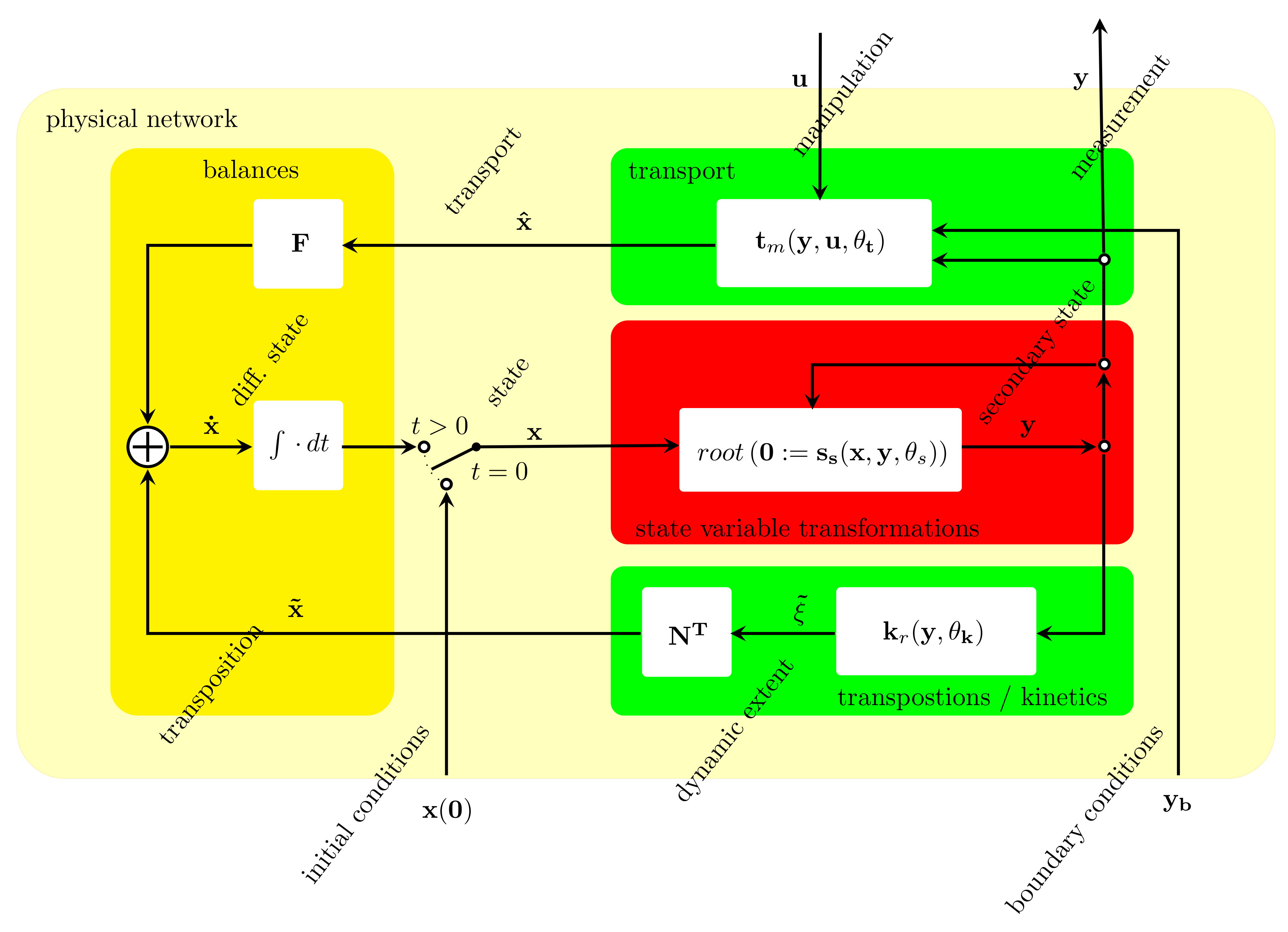
If one draws up the scheme defining the model, one quickly recognises that one part is missing. For these reasons, the missing piece is often called ”closure”, which, by their nature, are state variable transformations. Looking at a diagrammatic representation, Figure 2 shows the mathematical representation of a generic deterministic physical system, with x being the ”state” of the system in the form of a block diagram also showing the connections for a control system. The scheme has four external connections: the initial conditions x(0), the boundary conditions y_b and the two connections to the control system, namely, the manipulated variables u, the measurement y.

The dark-yellow box on the left indicates the balances and conservations. If the state is limited to the conserved quantities, then the yellow box is the conservation, and otherwise there is a balance. The green box on the top represents the transport laws for the extensive quantities, and the lower green box the reactions or transposition. Both are a function of a class of variables, which we call “secondary states”. Typical members are the quantities driving the transport of extensive quantities, namely temperature, pressure and chemical potential, while concentration defines the probability function in reaction kinetics. It is the red box that closes the gap between the state and the secondary state. The red box’s main components are thermodynamic models relating the extensive state to the intensive properties and geometrical relations that link geometrical variables to volume. The main physical–mathematical underlying frameworks are Hamiltonian systems for mechanical and contact geometry for the thermodynamic parts. Both define a configuration space. While classical mechanics is well established, contact geometry does not enjoy similar popularity. The energy formulation reads

$$U\left(S,V,\underset{¯}{\mathbf{n}},\frac{\partial U}{\partial S},\frac{\partial U}{\partial V},\frac{\partial U}{\partial \underset{¯}{\mathbf{n}}}\right)$$

(1)

with the last three elements being the temperature T, the negative pressure p and the chemical potential $\mu$. The thermodynamic configuration space is the assembly, including $U,S,V,\underset{¯}{\mathbf{n}},\frac{\partial U}{\partial S},\frac{\partial U}{\partial V},\frac{\partial U}{\partial \underset{¯}{\mathbf{n}}}$. An early introduction can be found in [9], followed by [10,11,12], which provides an extensive exposition of the subject.

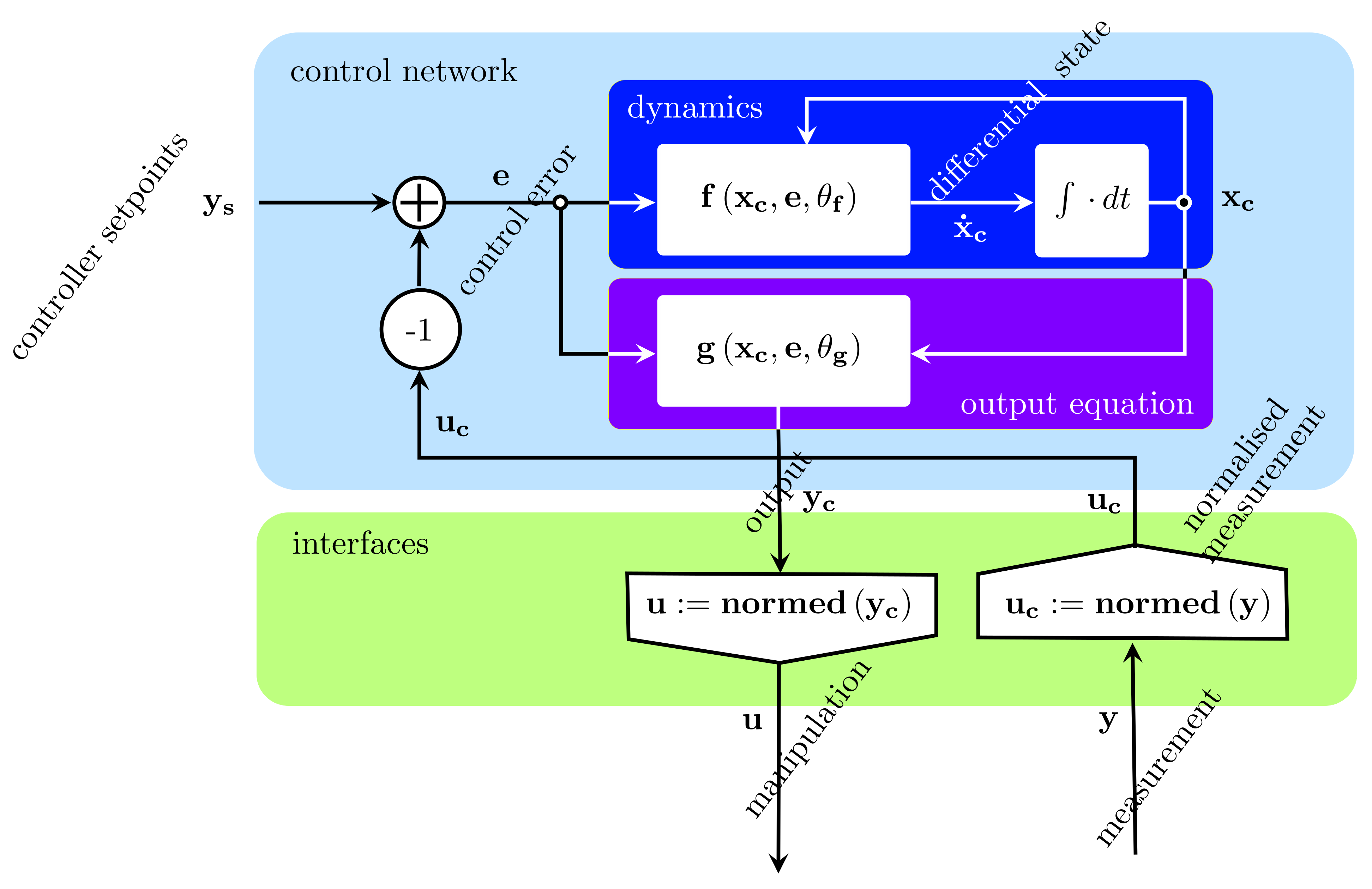
Processes are controlled. A single-layer control scheme may be of the form shown in Figure 3. Some of the variable classes are different from the ones in the physical system. There is still the state and the differential state. One now has to classify outputs and inputs, setpoints and control error. Figure 3 also shows the interfaces transferring state information in one direction, with control settings in the other direction, with the latter also being a function of the controller state via the output function.

The two examples demonstrate that the variable classes are domain-specific. While one can streamline things to some extent by using a state-space approach, one needs to adapt the variable classes to the disciplines to effectively support the process of defining the variable and equation system.

5. ProMo Ontology

The previous sections provide the main elements used to define the structure of the ProMo ontology. The top definition is the tree of disciplines. For each discipline, we must define elements associated with the structural elements enabling efficient handling of the building blocks and the elements that provide the framework for defining each building block’s behavioural equations.

We do not aim at generating a global ontology for all processes. Even if this was a feasible undertaking, the argument here is the improved targeting of groups of modellers (see also the discussion in Section 3), at least not in the first instance. Another argument is flexibility. An ontology is a living structure and will change with time, continuously aligning with new requirements. It is for these reasons that ProMo has its own ontology structure and a corresponding editor.

The organisation of the disciplines follows a couple of simple rules:

• Networks that house the same tokens are in an intra-relation;
• Networks that do not house the same tokens are in an inter-relation;
• Each discipline has its own branch;
• Disciplines may have subdisciplines.

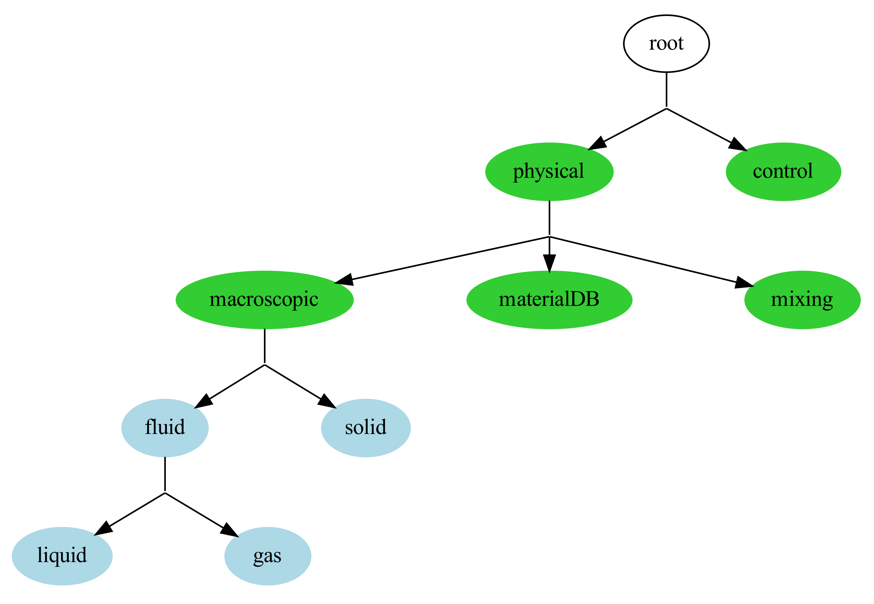
The sample ontology Figure 4 shows the discipline tree of an ontology designed for modelling a large group of macroscopic processes. The green disciplines are in an inter-relation, while the blue ones are in an intra-relation. On the top level, the ontology includes a physical and a control branch. We have the generic macroscopic systems, the material descriptions, and an example of a mixing domain devoted to empirical mixing models on the physical level.

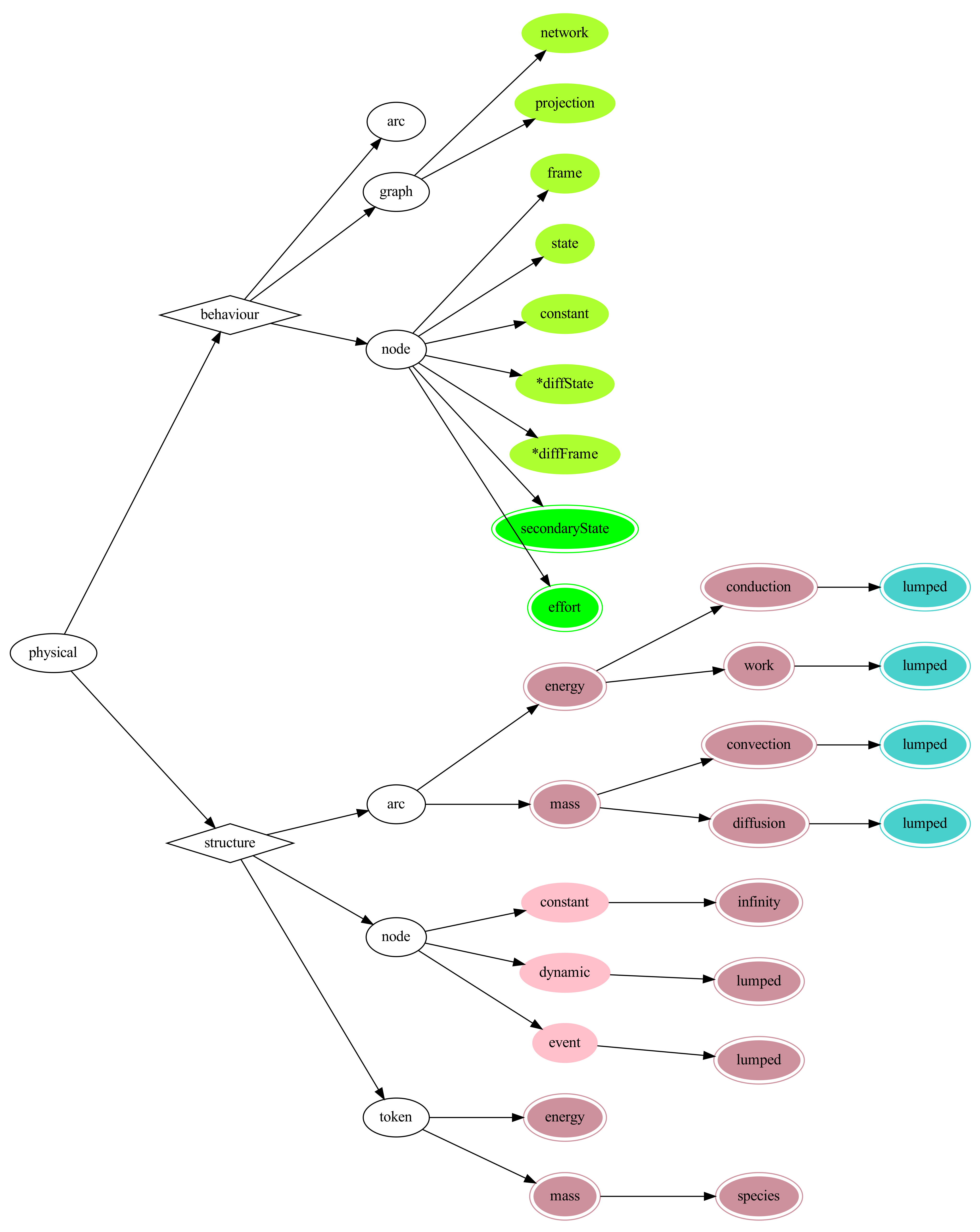
Each node has two branches of definitions: the branch associated with defining the process models’ structure and the branch with the definition of the variable classes. Figure 5 shows the definition of the root of the discipline tree.

The overall system is defined as dynamic with basic entities belonging to all three time-scale domains. For the representation of the network structures, we declare the variable class “network” and “projection”. Both are associated with the “graph”, the network. For the system theoretical definitions of the model equations, one defines the variable classes “frame” for the free variables, “state” and “constant”. The two additional classes are currently explicitly defined, namely, classes associated with the spaces generated by differentiating the states and frame variables. These definitions are required because of the design choice of uniquely identifying the dimensions of all mathematical objects. The issue of indexing has been introduced and discussed in [1].

Moving down the discipline tree, one can extend and augment the definitions. Figure 6 shows the example of the node labelled with “physical”. Thid is the parent to the nodes “macroscopic”, “materialDB” and “mixing”. It augments variable classes with “secondary state” and “effort”. The former appears in the generic representation of the dynamic physical system, Figure 2, while the term “effort” is a class that captures the effort variables [13], also called the conjugates to the thermodynamic potentials or generalised forces. In the context of contact geometry Equation (1), the temperature, the pressure and the chemical potential are three elements of the odd configuration space [9,10].

The structure includes the extension of the nodes, which applies to all nodes in the tree. It captures the time-scale property of capacitive elements and details it with the distribution effect.

6. Entity Behaviour

6.1. Equations

The ontology intrinsically defines the basic entities in the discipline-specific frame. For physical systems, this is the frame spacetime, while for control, the frame is usually limited to time.

ProMo’s equation editor can enter and edit the mathematical behaviour description. As mentioned above, we start with a set of ”port” variables: the constants, the frame variables, and the variables defining the configuration spaces’ base. We define a small, tailored language to enter the equations, namely, a variable defined by an expression. The description of the language and the mechanisms associated with implementing the details is beyond this paper and will have to be reported separately. Further information can be found in [3]. Thus, in very brief terms: The equation editor implements a parser and a template machine. The parser generates an abstract syntax tree, and the template machine uses the abstract syntax tree and generates different compiled versions of the equations, including LaTex rendering of online documentation. The main features of the parser are that it implements the index (For the discussion on the indexing, we refer to [1]) and rigorous unit handling.

The variable/expression bipartite multi-graph: We construct the equation system starting with the ”port” variables: frame, constants and the state variables. For physical systems, the base state variables are the ones defining the configuration spaces. The state variables appear in the block diagrams Figure 2 and Figure 3 after the integral. We then follow the paths in the respective block diagram. For physical systems, shown in Figure 2, the next step is to define the equations representing the red box, labelled with ” state variable transformations”, whereby each equation can only be a function of already defined variables. For the control system, these are the nonlinear dynamic function and the nonlinear static output function.

We allow for the definition of more than one equation for the same variable. This approach allows us to implement the basic thermodynamic variables, for example, temperature as a partial derivative of internal energy with respect to entropy. Variables with an implicit model equation must first be defined with an explicit model equation. Only then can the implicit model be added. This enables the proper handling of indexing and unit handling. Further details can be found in [3].

6.2. Graphical

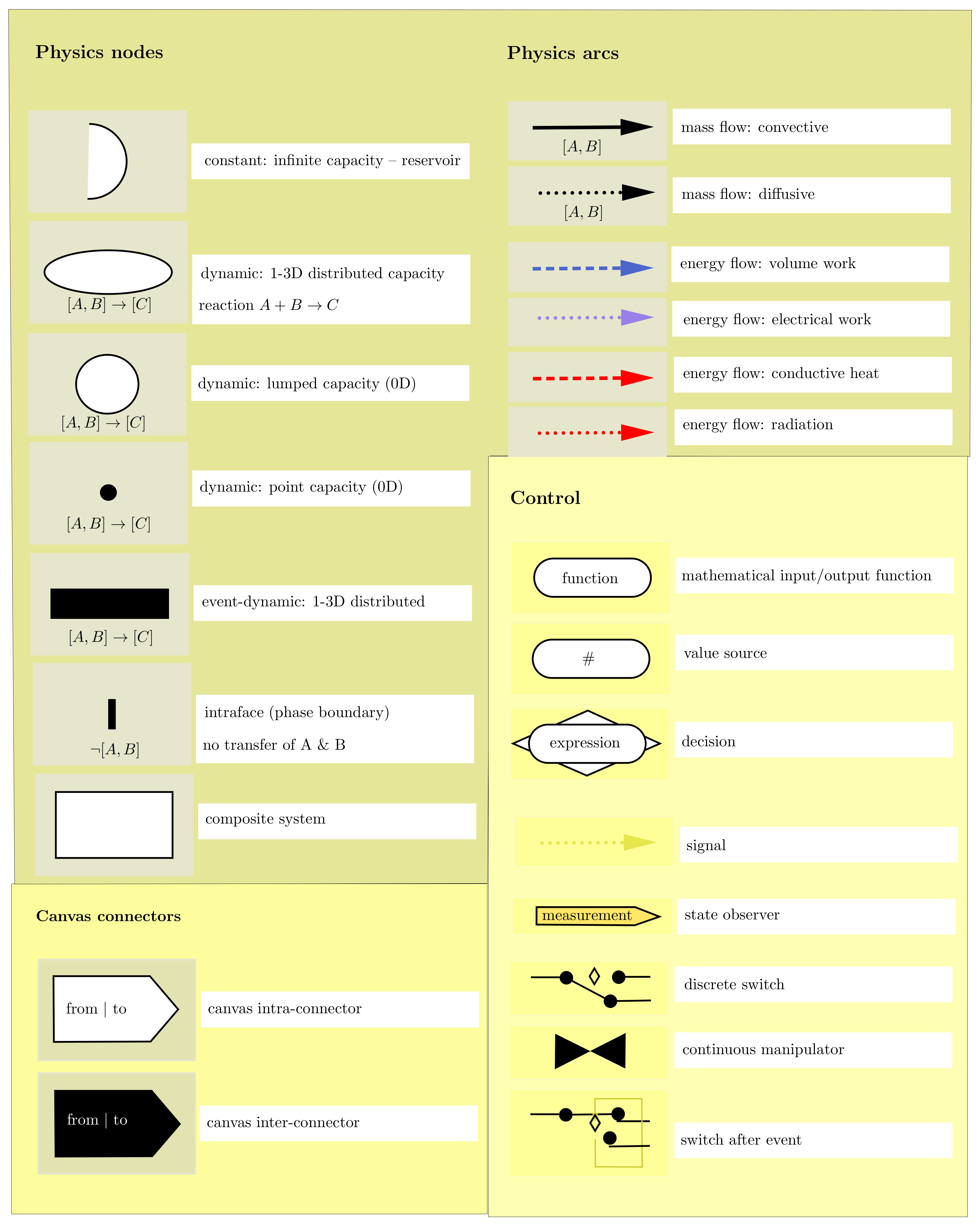
The ontology defines the base entities, and the equations describe the behaviour of these entities. For the physical systems, we have combinations of the time-scale behaviour, the distribution effects and the present tokens. By linking the mathematical behaviour description to graphical symbols, we generate a visual modelling language, to which the remaining paper shall be devoted. The graphical language uses a small number of visual symbols. For each discipline, a few capacity components and a few transport components remain to be defined. Appendix A shows a table of symbols for macroscopic physical systems and control.

The structure of the model, in terms of its composition of basic building blocks, is the main model-design issue, and not the equations. We can define the basic blocks’ behaviour, except for the specific material models, which have to be injected at the initialisation stage. A very elegant solution has been suggested and realised by Bjørn-Tore Løvfall’s PhD documented in his thesis [14]. He constructs one of the energy functions, usually Helmholtz, from two state equations, which serve as models of the specific material’s behaviour. Legendre transformation provides the additional energy funtions. The properties then are defined by derivatives of the surface with respect to state-dependent variables. Automatic differentiation makes the sytem tick.

The graphical language is an excellent model design tool. We not only teach it in our modelling course, we also use it extensively in projects to discuss the model structure. We shall now discuss a few examples.

7. Graphical Model-Design—Three Examples

This section discusses three examples demonstrating the power of the graphical model design and their use in ProMo’s model composer. An explanation for graphical symbols is in Appendix A.

7.1. Stirred Jacketed Tank

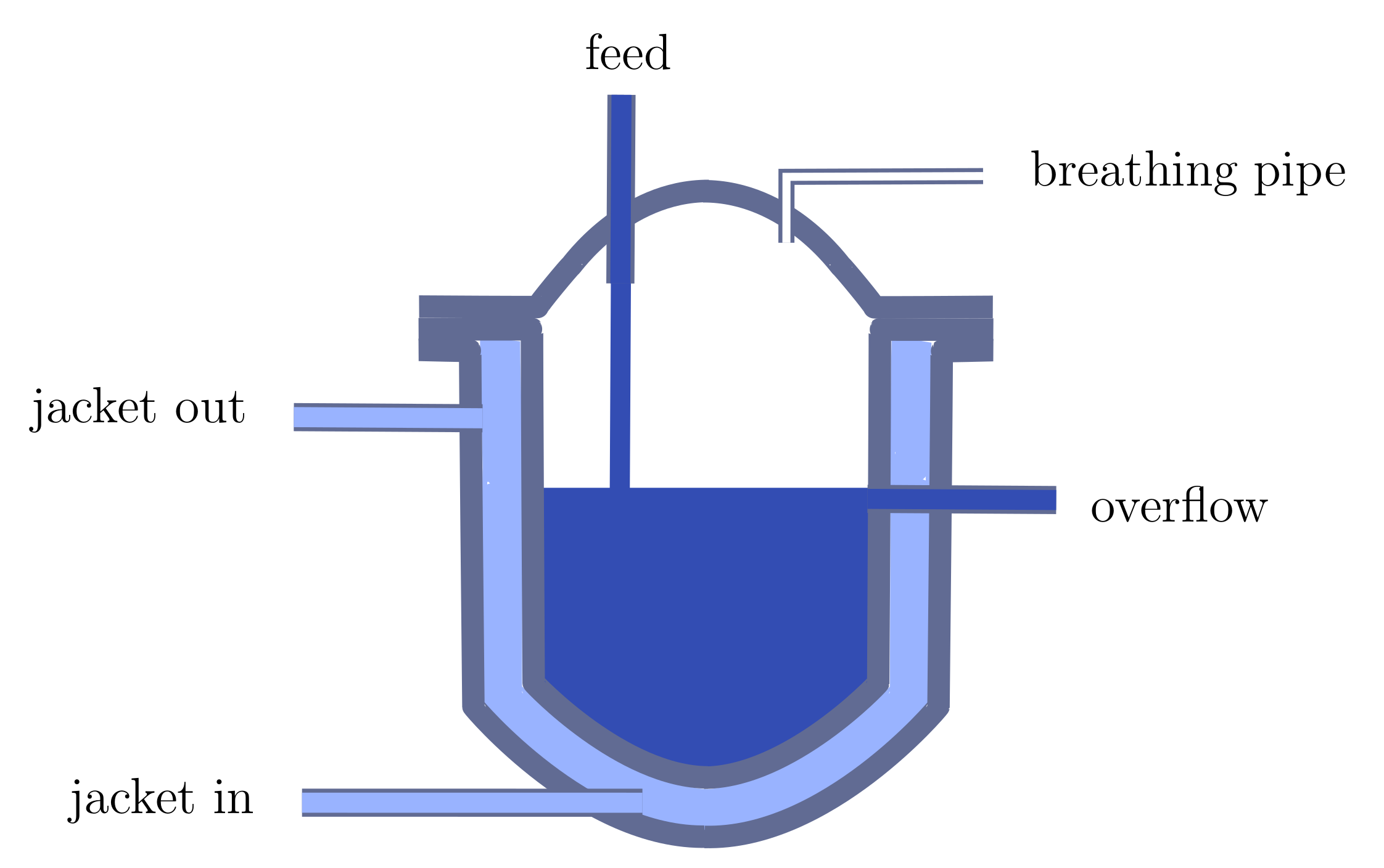
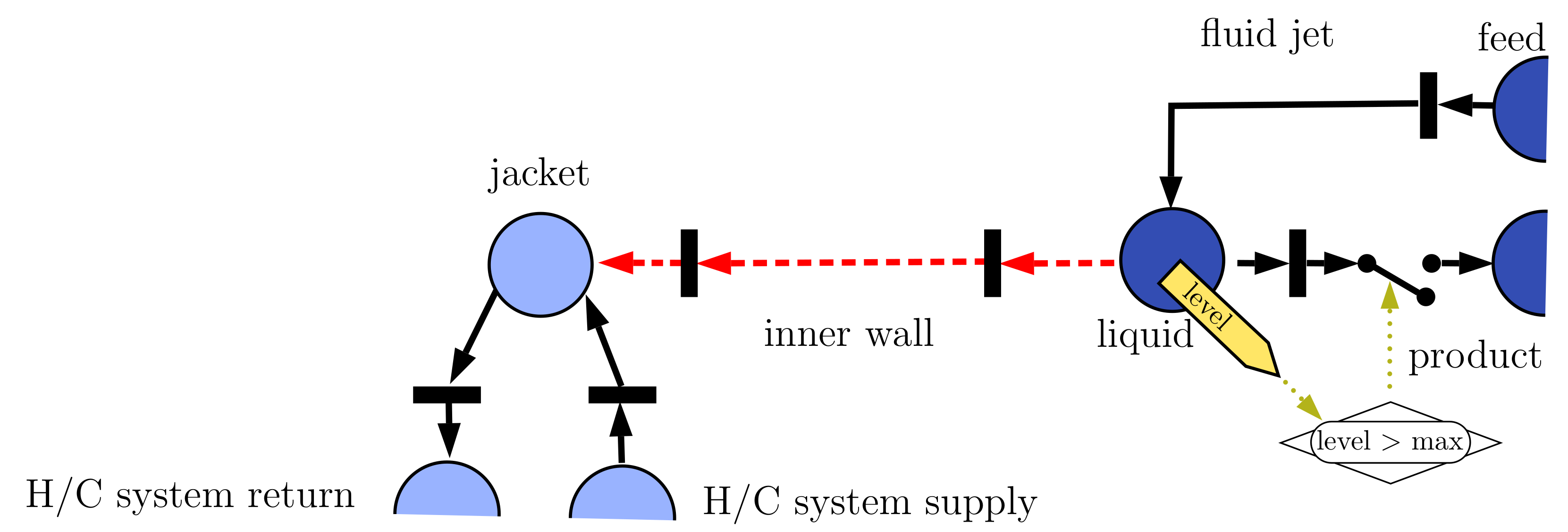
First, we look at a standard piece of equipment, the stirred tank reactor. Figure 7 shows a possible configuration.

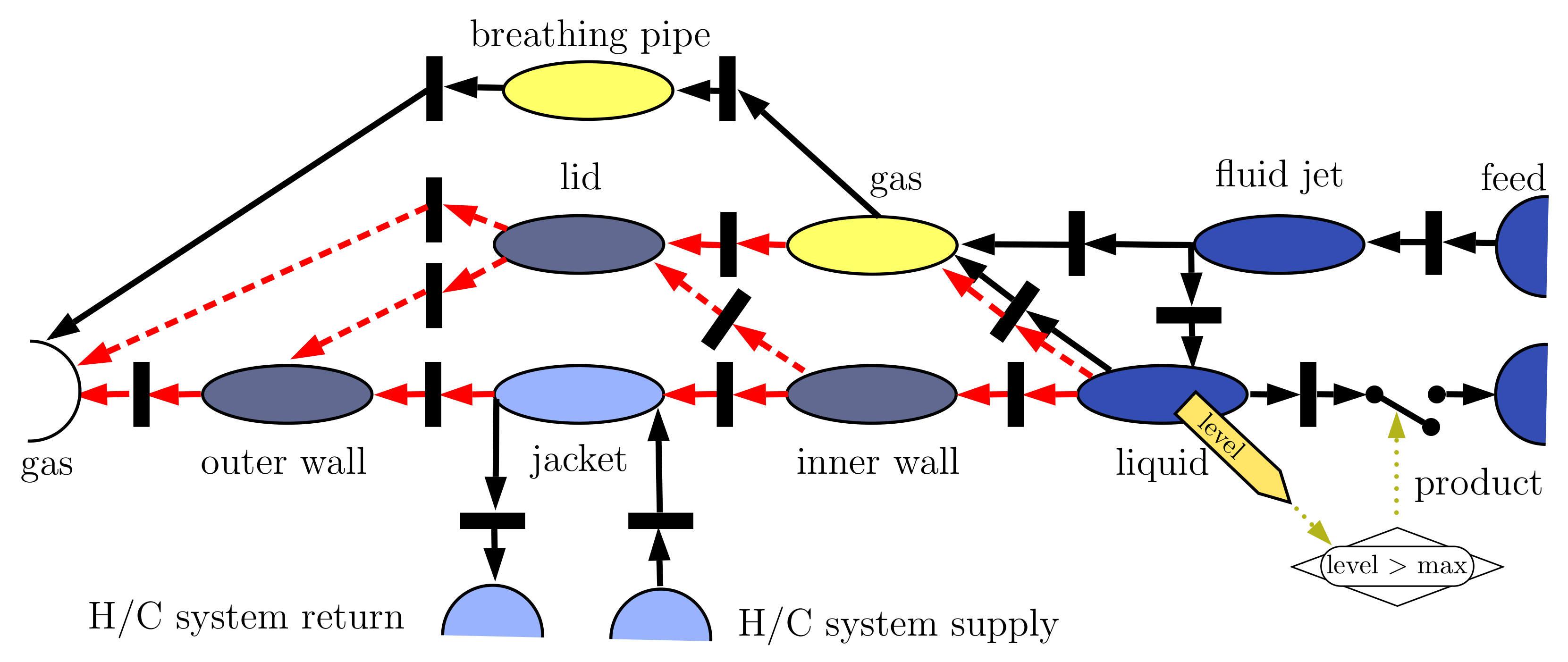
The tank is connected to one liquid feed, has an overflow, and is ”breathing” to the outside. The jacket controls the temperature of the contents. Figure 8 shows a relatively detailed model for energy flows but a relatively simple model for the reaction fluid.

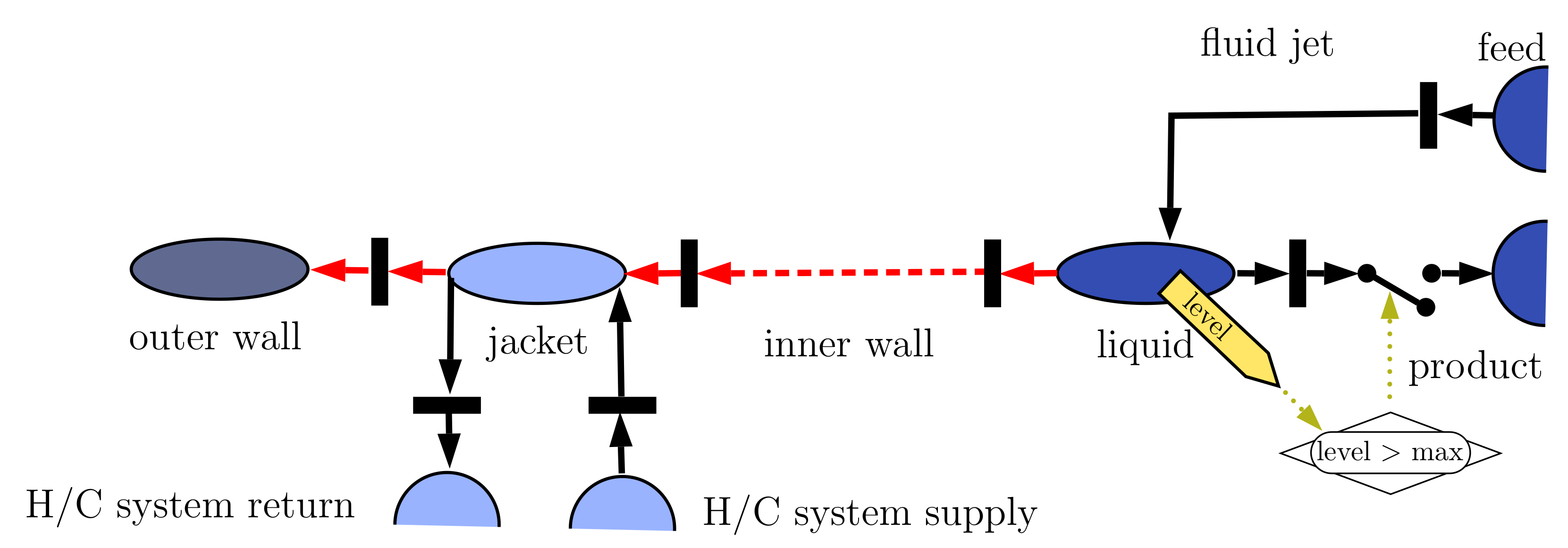
The overflow is of interest: an imaginary controller switches the overflow on when the level in the tank has reached the maximum. In the following examples, we use this approach of ”control” to handle events that change the configuration of the model. The controller shown in Figure 8 is not real, but implements the event of reaching the fluid level in the tank when the overflow begins to become active. The graphical language also enables model reduction or model simplification. Different applications require different details, and rougher or finer granularity. We can apply a series of assumptions:

• The shell is well insulated from the room and heat loss through the outer shell is insignificant;
• The fluid jet is very fast;
• The lid is well insulated from the lower part of the tank;
• The lid, gas and fluid are at about the same temperature as the room. The heat loss through the lid is insignificant;
• The inner wall conducts very well;
• The material exchange of the gas phase with the room is insignificant;
• The fluid jet is event-dynamic.

This helps us to achieve a significant simplification, shown in Figure 9.

One can simplify the model further by assuming:

• The outer shell has a negligible capacity;
• The contents is ideally mixed—thus, mixing is very fast, resulting in uniform conditions;
• The fluid flow in the jacket is extremely fast—yielding uniform temperature in the jacket.

This yields a much more simple model, as shown in (Figure 10).

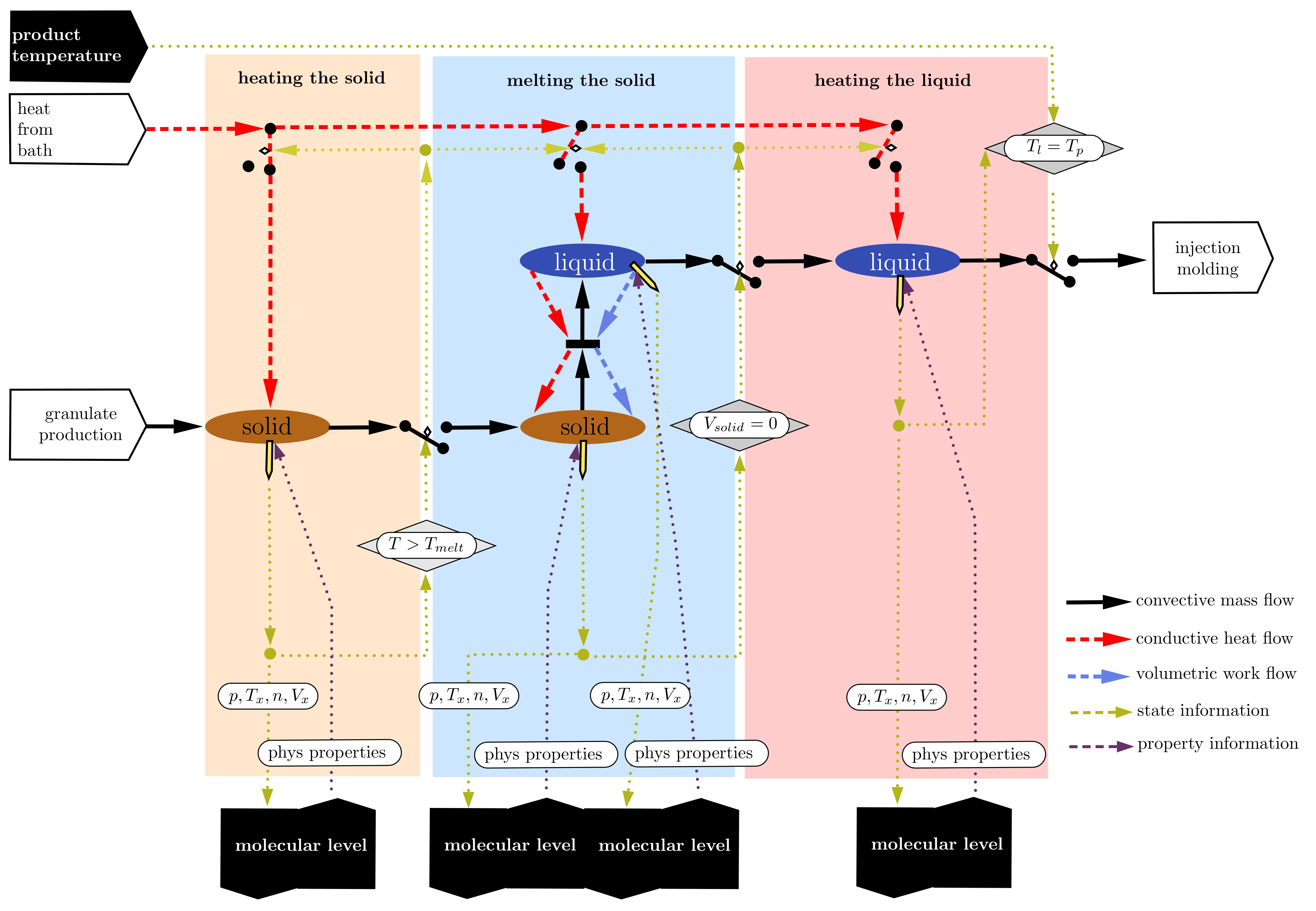
7.2. Melting Process

This second example focuses on ”model control”. It shows the melting of a solid as shown in Figure 11. The process itself is rather straightforward: a solid is exposed to a heat source and heated up. Once the melting temperature at the hot surface has been reached, a liquid phase is generated. The model switches to describe two phases, assuming that the solid has no direct contact with the hot surface, and a liquid film is in between the solid and the surface. The liquid’s thermal distribution effect can be quite complex, and is not shown at this level of description.

The topology indicates a connection to molecular modelling, which, as shown, implies close coupling, thus running the molecular modelling task at every point in time. Molecular codes are notoriously computationally intensive and slow. There is at least one unique method, COSMO [15], which works for some configurations well and is fast. Close coupling is not an option for the codes that minimise a vast number of molecules’ overall energy. In these cases, the approach used replaces the molecular modelling module with a surrogate model that spans the variable space sufficiently and is of a simple structure. The molecular modelling task is replaced by an input/output function with the property function in a subspace of the fundamental variables, such as $p,T,n$.

7.3. Moving Boundary Problem

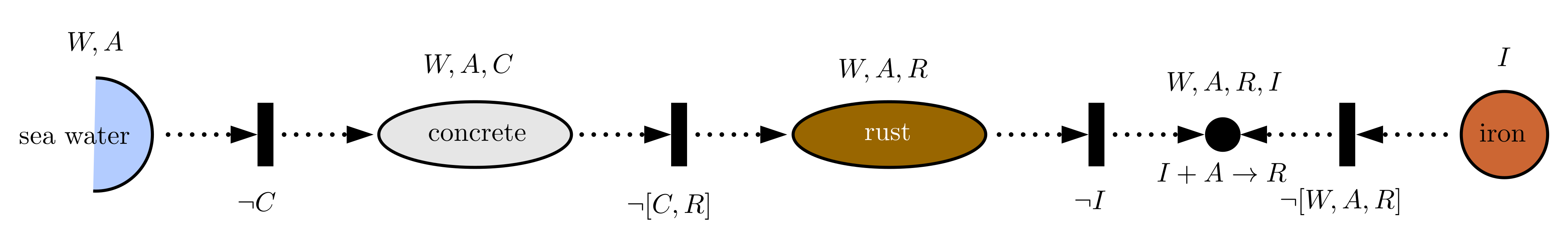
Many processes are characterised by one part of the material growing at the cost of another. We take the example of a corrosion process: an iron-rod-reinforced concrete pillar in water. The problem is well known and of broad interest. Water, carbon dioxide, chlorine anions and oxygen mainly diffuse into the concrete and cause the iron to oxidise, resulting in a loss of strength over time. Since it is not the reaction that is of interest, Figure 12 shows a model representing the process with a simplistic abstract reaction. The main issue, in this case, is to demonstrate the approach used to model moving boundaries.

The reaction is placed into an infinitely small reaction front, represented by an infinitely small volume where the reaction occurs, and the point capacity is combined with restrictive intrafaces to the left and right. The rust is transported to the left, while iron comes from the right. The species water, active component and rust do not transfer into the iron $\neg [W,A,R]$, and iron is not transferred to the rust $\neg \left[I\right]$. Rust and concrete are not transferred between the rust and the concrete domain, and concrete is not transferred into the water.

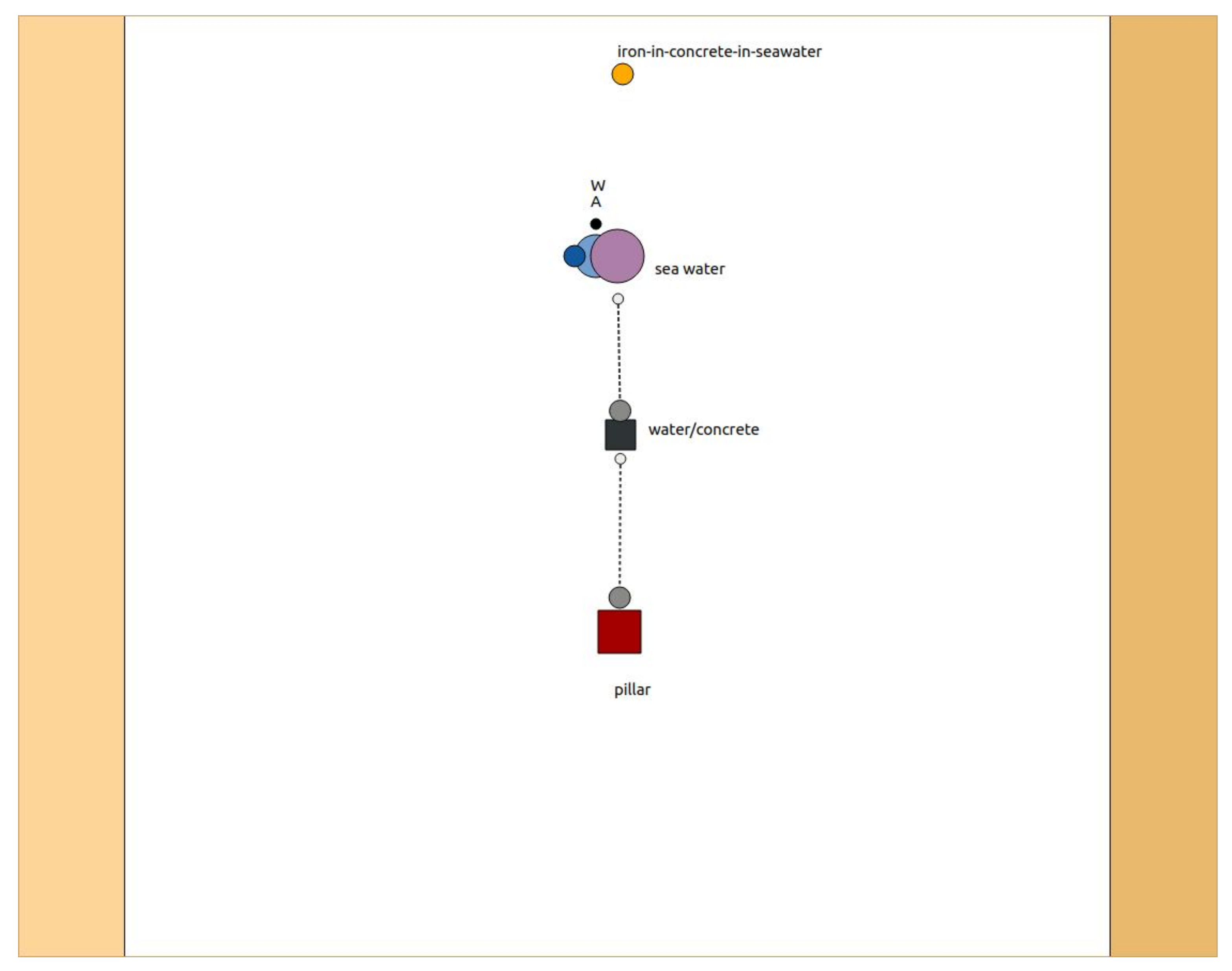
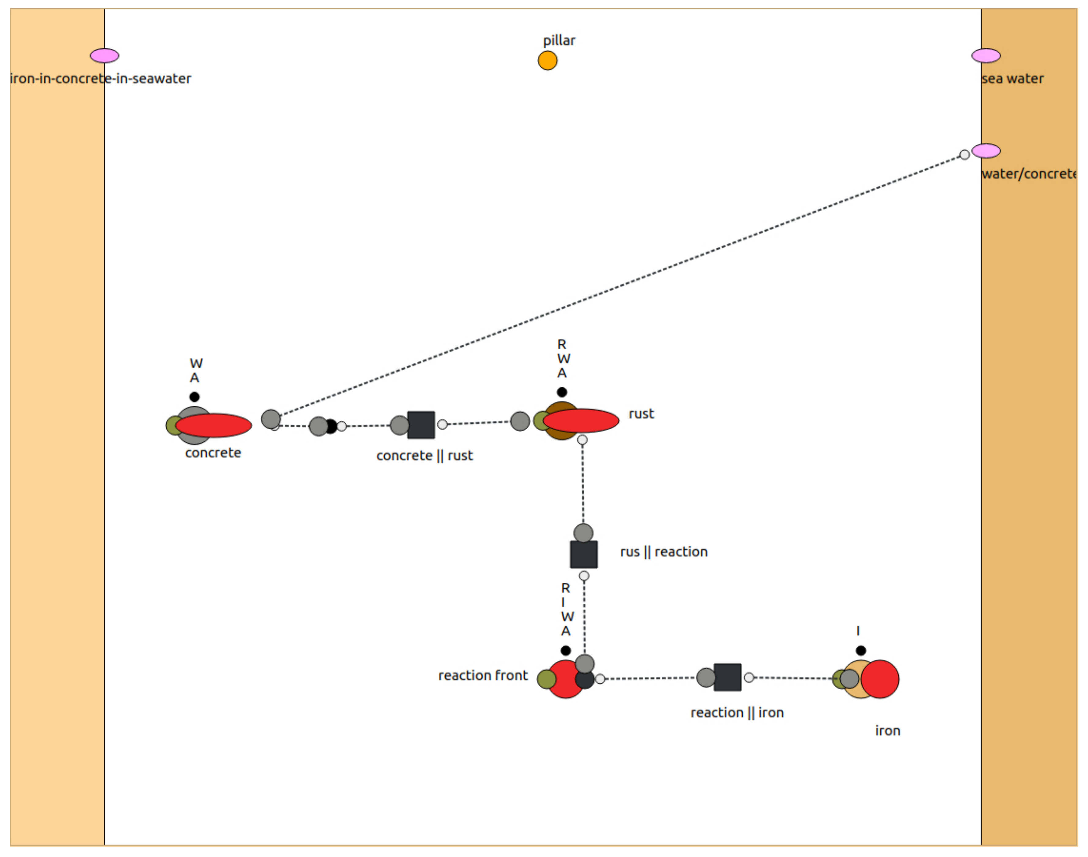
The Figure 13 and Figure 14 show two pictures taken from ProMo’s model composer. Figure 13 shows the top layer, while Figure 14 shows the model of the pillar with the iron embedded in concrete and the reaction front receiving iron from the iron bar, converting it into rust, which is transported to the rust node, representing the rust capacity.

The ProMo software uses simple graphical objects limited to ellipses and rectangles for visual representation. Decorators are used to indicate the membership to networks—liquid and solid in the example—in the form of circles. The membership to specialised networks, like concrete, rust or iron, is indicated by coloured circles. ProMo provides an editor that allows the user to design the graphical object. Arcs are directional, with the tail as a small circle and the head a larger and darker circle. Intrafaces are the black squares.

7.4. Other Applications

The reader may be interested to learn that we used this graphical approach for very many different processes. In process modelling lectures, we discuss tanks, mixing models, heat exchangers, distillation, chicken coop and greenhouses and wood drying and fruit transport, life-support systems, fermentation processes, biological cells, water treatment plants, solar reactor, mammal blood flow, moving bed reactor, decaffeination plant, a methanol plant, laboratory equipment like Soxhlet, mokka maker, crystaliser, bubble column, etc.

We used the same approach in European projects, including the modelling of polyurethane foams, production of high-precision ceramic products, biorefining processes, wastewater cleaning plants, transport of fruit and vegetables, life-support systems for space travelling, membrane processes, catalytic bed reactors, coating processes, etc.

8. Conclusions

Motivated by reductionism, models are seen as directed ”networks”, where abstract ”tokens” live in nodes and move about through arcs. The concept of ”tokens” allows us to apply the network concept to different disciplines, thereby enabling the multi-disciplinary and multi-scale model building process. The nodes are then capacities for the tokens, and the arcs’ transport tokens.

For physics, the tokens are first the conserved quantities that form the basis of the Hamiltonian’s and the contact geometry’s configuration space. Since we also model reactive systems, the tokens are extended to refining mass with species, consequently augmenting the representation with balances. This approach thus captures the physical system on all levels, including electronic and atomic, and particulate and macroscopic systems. For some particulate processes, the behaviour description is augmented with population balances. For financial systems, the tokens are monetary values. The node represents an account, with the monetary value being the state, and interest plays the role of a production term similar to the role that reactions take in component mass balances.

Reductionism is applied recursively, resulting in a hierarchical representation of the modelled process. The subdivision is continued until a basic level is reached, where ”basic” implies that it can be considered a basic building block. The definition of ”basic” is the smallest granules in the decomposition process, such that the resulting model serves the intended purpose.

ProMo implements an ontology, which captures the knowledge of a user-defined application domain, which, in turn, reflects the hierarchy of disciplines considered for the application domain. For each discipline, the ontology defines the infrastructure for the definition of the model structure and the behaviour description, with the latter being a multi-bipartite graph of variables and their defining relations. This bipartite graph captures the behaviour of each basic building block for all involved disciplines. The variable/expression set is lower triangular in the sense that one begins by defining the state that reflects the relevant tokens in a node. We allow for multiple definitions of the variables, thereby supporting the use of principle definition equations as well as more practical versions, which ultimately enables the substitution of a complex with a simple model, also termed the ”surrogate”.

The ProMo suite resolves a number of issues in process modelling:

Incompleteness and consistancy: The systematic approach of constructing the variable/expression system guarantees the completeness of the model equations. The fundamental base used to describe the entity’s behaviour models is tiny, namely, the thermodynamic and mechanical system’s configuration space. Physical units and dimensionality is defined only for the fundamental quantities. They automatically propagate when defining new variables.

Code generation: is automated and does not require manual intervention. The entity behaviour code is centralised and not distributed over unit models, as this is commonly the case in chemical engineering software.

Documentation: The expressions defining a variable are compiled as part of the definition process. Consequently, the documentation is complete and available during definition time.

Closure: Defining the fundamental behaviour equations as the conservation equations has two main advantages: (i) the equations are not substituted, and (ii) the closure of the balances can be guaranteed for the defined accuracy.

The graphical model-design language: enables us to capture the structure of the modelled process and generate alternatives quickly. The simplicity makes it an efficient discussion tool for exploring functionality, required detail, involved disciplines, and complexity to generate alternatives.

References

- Preisig, H.A. Constructing and maintaining proper process models. Comput. Chem. Eng. 2010, 34, 1543–1555. [Google Scholar] [CrossRef]
- Harold, M.P.; Ostermaier, J.J.; Drew, D.W.; Lerou, J.J.; Luss, D. The continuoulsy stirred decanting reactor: Stead state and dynamic features. Chem. Eng. Sci. 1996, 51, 1777–1786. [Google Scholar] [CrossRef]
- Elve, A.T.; Preisig, H.A. From ontology to executable program code. Comput. Chem. Eng. 2018. [Google Scholar] [CrossRef]
- Lind, S.; Rogers, B.; Stansby, P. Review of smoothed particle hydrodynamics: Towards converged Lagrangian flow modelling. Proc. R. Soc. A 2020, 476. [Google Scholar] [CrossRef] [PubMed]
- CEN Workshop Committee. CEN/WS MODA-Materials Modelling-Terminology, Classification and Metadata (CWA 17284); CEN Workshop Committee: Brussels, Belgium, 2018. [Google Scholar]
- Bernhard, P.; Deschamps, M. Kalman 1960: The birth of modern system theory. Math. Popul. Stud. 2019, 26, 123–145. [Google Scholar] [CrossRef] [Green Version]
- Willems, J.C. The behavioral approach to systems theory. In Proceedings of the Conference on New Approaches in System and Control Theory, Istanbul, Turkey, 2005; pp. 59–71. Available online: https://homes.esat.kuleuven.be/~sistawww/smc/jwillems/Articles/ConferenceArticles/2005/7.pdf (accessed on 17 March 2021).
- Caratheodory, C. Untersuchung ueber die Grundlagen der Thermodynamik. Math. Ann. 1909, 67, 355–386. [Google Scholar] [CrossRef] [Green Version]
- Peterson, M.A. Analogy betwween thermodynamics and mechanics. Am. J. Phys. 1979, 47, 488–490. [Google Scholar] [CrossRef]
- Rajeev, S.G. A Hamilton–Jacobi formalism for thermodynamics. Ann. Phys. 2007, 323, 2265–2285. [Google Scholar] [CrossRef] [Green Version]
- Bravetti, A. Contact Hamiltonian Dynamics: The Conceptand Its Use. Entropy 2017, 19, 535. [Google Scholar] [CrossRef]
- Bravetti, A. Contact geometry and thermodynamics. Int. J. Geom. Methods Mod. Phys. 2019, 16. [Google Scholar] [CrossRef]
- Breedveld, P.C.; Rosenberg, R.C.; Zhou, T. Bibliography of Bond Graph Theory and Application. J. Frankl. Inst. 1991, 328, 1067–1109. [Google Scholar] [CrossRef]
- Løvfall, B.T. Computer Realisation of Thermodynamic Models Using Algebraic Objects. Ph.D. Thesis, NTNU, Trondheim, Norway, 2008. [Google Scholar]
- Klamt, A. The COSMO and COSMO-RS solvation models. WIREs Comput. Mol. Sci. 2018, 8, e1338. [Google Scholar] [CrossRef]
Figure 1.
Network of networks representation of multi-disciplinary model graphs.
Figure 2.
A generic dynamic physical system.
Figure 3.
A generic control system.
Figure 4.
A sample discipline tree. It is designed to capture a very wide range of processing plant models. The green nodes are in an inter-relation, and thus transfer tokens, while the blue ones are in an intra-relation, and thus transfer state information.
Figure 5.
The root node in the discipline tree. It has two branches: the structure branch is used to define the ontology items used for designing the items associated with capturing the model as a directed graph; the behaviour branch serves the purpose of defining the variable classes used to capture the mathematical description of the entity behaviour models.
Figure 6.
The physical node in the discipline tree. Both branches are expanded with additional items. In the structure branch, the basic entities are populated with tokens and specified with the modelled distribution effects.
Figure 7.
The configuration of a jacket tank with an inflow, an overflow and a breathing pipe for pressure compensation.
Figure 8.
A relatively complex model without condensation on the lid.
Figure 9.
A simplified tank model. No heat loss through the outer shell, lid and gas phase; “breathing” is neglected, jet is event-dynamic.
Figure 10.
An even more simplified tank model. The outer wall is neglected and jacket, and the contents are lumped.
Figure 11.
A generic melting process demonstrating how the model switching is included in the model, leading to a surprisingly complicated overall model.
Figure 12.
Rusting iron in concrete is an example of a moving boundary problem. The top row shows the species present in the respective capacities, while, in the lower row, the transfer constraints for the intrafaces and the reactions in the point capacity are shown.
Figure 13.
Rusting iron in concrete, a view of the ProMo’s graphical modeller showing the top of the hierarchy with the pillar in the seawater. The seawater is modelled as a reservoir system (large mauve circle) with two circular indicators attached, as seawater is a liquid. The black dot indicates mass, and the ”W” and “A” stand for the species water and active component.
Figure 14.
Rusting iron in concrete, a view of the ProMo’s graphical modeller showing the pillar model. The concrete and rust are modelled as distributed systems (ellipses). The reaction front is modelled as an infinitely small lumped system (black dot), decorated with the large red dot indicating the reaction front and the green dot indicating the solid. The iron is modelled as a lumped system. “R”, “I” stand for the species rust and iron. The left strip elements show the parents, while the ones on the right are the siblings in the hierarchy.
Publisher’s Note: MDPI stays neutral with regard to jurisdictional claims in published maps and institutional affiliations. |
© 2021 by the author. Licensee MDPI, Basel, Switzerland. This article is an open access article distributed under the terms and conditions of the Creative Commons Attribution (CC BY) license (http://creativecommons.org/licenses/by/4.0/).
Share and Cite
MDPI and ACS Style
Preisig, H.A. Ontology-Based Process Modelling-with Examples of Physical Topologies. Processes 2021, 9, 592. https://0-doi-org.brum.beds.ac.uk/10.3390/pr9040592
AMA Style
Preisig HA. Ontology-Based Process Modelling-with Examples of Physical Topologies. Processes. 2021; 9(4):592. https://0-doi-org.brum.beds.ac.uk/10.3390/pr9040592
Chicago/Turabian StylePreisig, Heinz A. 2021. "Ontology-Based Process Modelling-with Examples of Physical Topologies" Processes 9, no. 4: 592. https://0-doi-org.brum.beds.ac.uk/10.3390/pr9040592
Note that from the first issue of 2016, this journal uses article numbers instead of page numbers. See further details here.