Gain-Scheduled Model Predictive Control for a Commercial Vehicle Air Brake System

Abstract

This paper presents a control-oriented Linear Parameter-Varying (LPV) model for commercial vehicle air brake systems with the electro-pneumatic proportional valve based on the nonlinear mathematical model, a set of discrete-time linearized models at different target pressures with the q-Markov Cover system identification method. The scheduled parameters for the LPV model were the brake chamber pressure, which was controlled by the electro-pneumatic proportional valve. On the basis of the LPV model, a family of Model Predictive Control (MPC) controllers with a Kalman filter was designed at each operation point. Then, the gain-scheduled MPC was designed over the entire operating range with the switched strategy, which was validated by experimental data. Furthermore, compared with the PID controller, the performance of the system was improved with a gain-scheduled MPC controller.

1. Introduction

The brake system as a vital part of a vehicle is an essential aspect of the vehicle dynamics, especially the longitudinal dynamics. Different types of power brake systems are used in vehicles, such as hydraulic brake systems, air brake systems, and air-over-hydraulic brake systems. The air brake system is widely used in commercial vehicles and has the characteristics of superior braking force, excellent reliability, easy maintenance, and a working medium without recycling. However, compared with the hydraulic brake system [1], the air brake system has a significant time delay performance, which can easily cause traffic accidents. One of the accident reduction strategies is to develop an advanced vehicle brake system [2].

For braking, an excellent response time, a shorter delay time, and a faster response time are always preferred [3]. The research on the theoretical knowledge of pneumatic and hydraulic brake systems is now very mature [3,4], but many theoretical studies only considered the static characteristics of the pneumatic system, such as the braking force distribution of the front and rear axles and the related braking performance. From the practical point of view, the instantaneous braking response needs to be considered. Therefore, research on the dynamic characteristics of the braking system is crucial. The characteristics of the vehicle dynamics of the braking system mainly focus on the brake pedal travel, response time, and braking distance [5]. Zamzamzadeh M. et al. [6] performed an analysis of the effect of braking pedal force on vehicle braking distance through a multi-body dynamic simulation based on the Single Unit Truck (SUT) model. The simulation results showed that there was a nonlinear relationship between the braking pedal force and the braking distance. Zhe Wang of Zhejiang University [7] used a servo unit to simulate the operation of the brake pedal to research the hysteresis characteristics of the pneumatic brake system of an eight-axle commercial vehicle under emergency braking. The results showed that there was a quadratic relationship between the delay time and the pedal opening.

A key point for improving the performance of the pneumatic brake system is to reduce the system response time with smooth braking torque. The apparent hysteresis characteristics of the air brake system are mainly caused by the compressibility of the gas, the delay of the multi-switching of the pedal valve, and the length of the brake line, which is limited in application to commercial vehicles. Relevant scholars worldwide have conducted many studies on this. Palanivelu S. [8] proposed a system modeling method based on the model design, established the model of each component of the pneumatic brake system—dual-chamber brake valve, quick release valve, relay valve, front and rear brake chamber—and obtained the transient pressure response, braking distance, and vehicle deceleration through the test data in the braking process. R He. et al. [9] established an AMESim model of the semitrailer braking system, including the relay emergency valve and chambers, to predict and control the response time, which was verified by an experiment. Vikas Gautam. et al. [10] developed an electric brake system widely used in commercial vehicles, to reduce the response time of the pneumatic brake system and shorten the stopping distance, and established the relevant mathematical model from the input voltage to the pressure transient, which was verified by experimental data. To improve the braking performance, active safety systems play a significant role in braking stability and brake response. The Anti-lock Brake System (ABS) [11], which was the first active safety system to improve braking safety, has become a critical component for vehicles. Later, the Traction Control System (TCS), ABS expansion [12], Electronic Brake Force Distribution (EBD), the Tire Pressure Monitoring System (TPMS), the Roll Stability Control system (RSC) [11], and the Electronic Stability Control system (ESC) [13] were also developed sequentially and have been widely used in passenger cars. The emergence of the Electronic Braking System (EBS) [14] has dramatically improved the safety of commercial vehicles.

However, braking is a complex multi-variable, nonlinear, and strongly coupled process. The problem can be solved better by wire control technology, and the major commercial vehicle brake technology developers and researchers in the world currently focus on electronic control brake technology [15]. To realize active braking, many feedback control schemes have been exploited. Chen Lin [16] compared the four-wheel hub-motor torque control method with the traditional single-wheel hydraulic brake control for the ESC system. The results showed that at high speed, the method of motor torque control was not effective as the hydraulic brake control. Zhu Bing [17] designed a set of active pneumatic brake actuators compatible with the traditional pneumatic brake system of semi-trailer trains and established a model-based active pneumatic brake control strategy, which was tested and verified. Hongyu Zheng [18] proposed a hierarchical structure controller and developed a Hardware-In-the-Loop (HIL) test bench of the electronic pneumatic brake system to validate the control strategy, which showed the effectiveness of the control strategy for a heavy tractor semi-trailer. Shuo Cheng [19] proposed a Lateral-Stability-coordinated Collision Avoidance Control System (LSCACS) based on Model Predictive Control (MPC) to improve the performance of collision avoidance and lateral stability. Wei Zhang [20] proposed a robust steering torque control strategy for the lateral tracking functionality of autonomous driving vehicles and utilized a gain-scheduling approach to achieve feedback gain, which can maintain the control system’s robustness.

Furthermore, for a highly nonlinear system, the Linear Parameter-Varying (LPV) system is used to obtain better nonlinear dynamics. The related modeling method and control strategy have been increasingly studied. Qu Shen [21] designed switched gain-scheduling LPV controllers with hysteresis switching logic using the Linear Matrix Inequality (LMI) convex optimization approach based on a switched LPV model. Tianyi He [22] proposed an innovative design of smooth-switching LPV Dynamic Output-Feedback (DOF) controllers and designed a family of LPV controllers on each subregion, as well as switching smoothness among adjacent subregions. Luca Cavanini [23] designed an MPC to drive a UAV based on the LPV model using a subspace identification technique. Rui Wang [24] solved an optimal control problem for aero-engines based on a switched LPV model and presented an optimal control method for the switched LPV system. However, there has been little research on the LPV model for the pneumatic brake system until now.

Since MPC can handle the control problems for nonlinear systems, it is currently a representative control method. MPC has the advantages of stability, robustness, and optimality. For different MPC controllers with different operating points, in this paper, a gain-scheduled MPC scheme was proposed to solve the control problem of brake pressure in the pneumatic brake system. Compared with the nonlinear model, the linear model had better real-time performance and was easier to analyze and calculate. However, highly nonlinear characteristics existed in the current pneumatic brake system, so the system identification method was adopted for model linearization.

The main contribution of this paper is the utilization of gain-scheduled model predictive control based on the LPV model with different operating points.

The paper is organized as follows. Section 1 describes the pneumatic brake system overview and control problem. Section 2 presents the control-oriented model, model linearization, and the LPV model. Section 3 designs the gain-scheduled MPC controller based on the LPV model. The simulation validation process is presented in Section 4. The experimental validation process is provided in Section 5. Conclusions are given in Section 6.

2. System Overview and Control Objective

2.1. The Pneumatic Brake System with the Electro-Pneumatic Proportional Valve

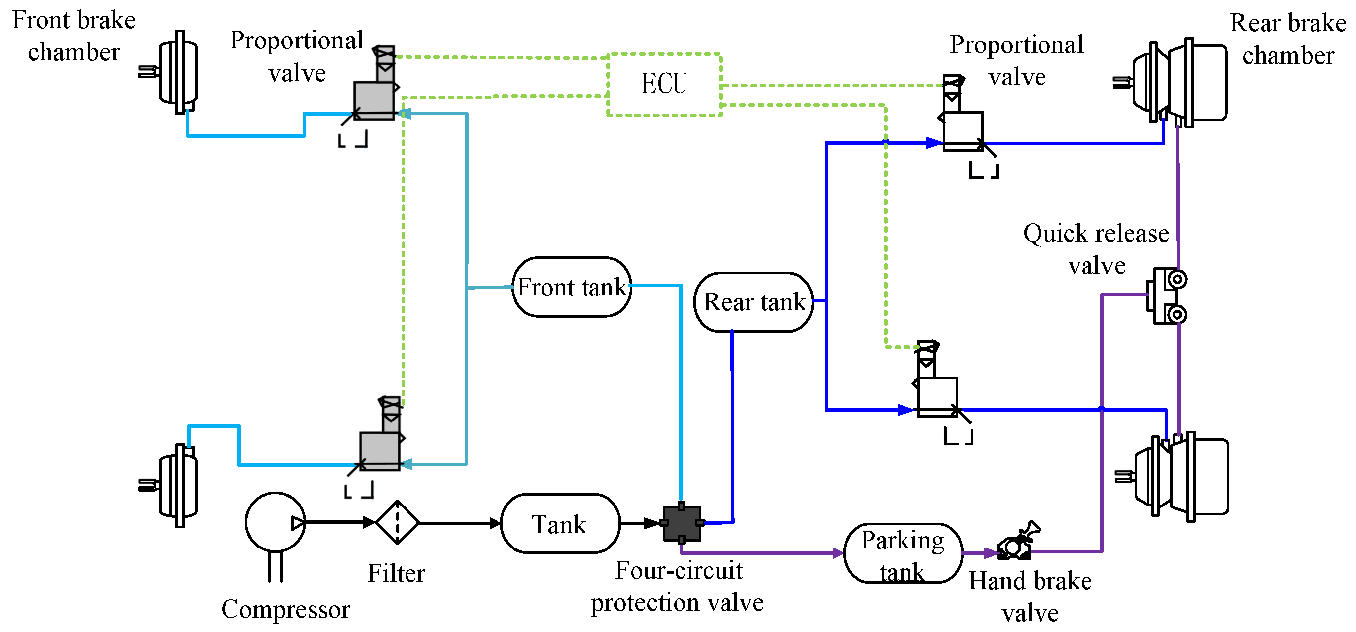
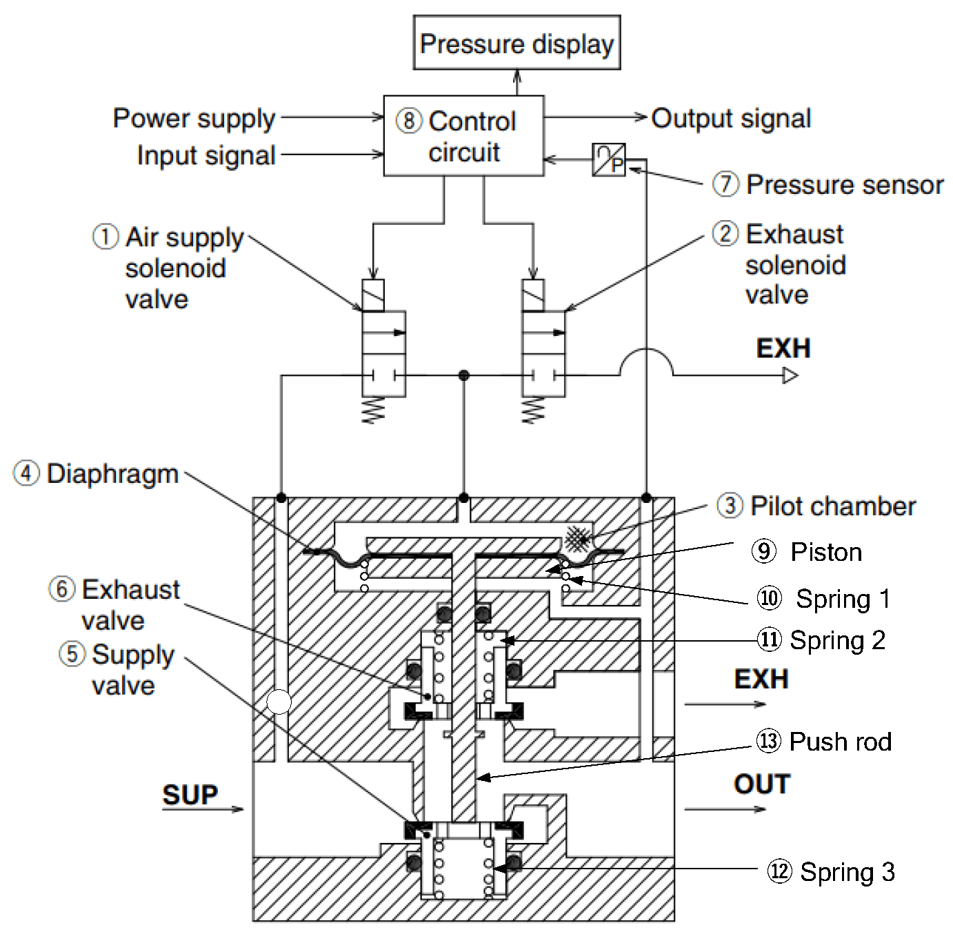
The pneumatic brake system was mainly composed of a compressor, air storage tank, dual-chamber brake valve, pedal valve, relay valve, brake chamber, etc. To reduce the system response time, vehicle brake distance, and realize active braking, the pneumatic brake system studied in this paper considered mainly two components: the electro-pneumatic proportional valve and brake chamber. The electro-pneumatic proportional valve in the electrical control circuit was paralleled in the original circuit-air control circuit (see Figure 1). The electro-pneumatic proportional valve used in this system was the ITV series from SMC Corporation [25], mainly consisting of a supply/exhaust solenoid valve, pilot chamber, spool, and spring (see Figure 2).

When the driver presses the brake pedal, the supply solenoid valve of the electro-pneumatic proportional valve opens, and the exhaust solenoid valve closes. The air from the compressor arrives in the pilot chamber through the supply solenoid valve. The pressure difference pushes the spool to move down. The air is allowed to go through the inlet port to the exhaust port, and the pressure of the brake chamber rises to achieve braking. Based on the detailed structure of the components, using fluid mechanics and dynamics equations, a nonlinear mathematical model of the pneumatic braking system for commercial vehicles from the input signal to the output pressure of the brake chamber was established.

2.2. Electro-Pneumatic Regulator Controller

The electro-pneumatic proportional valve has a local PID controller such that it is operated by providing the required pressure. The control circuit of the electro-pneumatic proportional valve can adjust the output pressure, which is proportional to the input voltage. The output of the local controller is shown as Equation (1) below.

$$\mathrm{u}\left(k\right)=K_{p}e\left(k\right)+K_I\sum _{i=0}^{k}e\left(i\right)T_s+K_D\frac{e\left(k\right)-e(k-1)}{T_s}$$

(1)

where $u\left(k\right)$ is the optimal control, k is the sample index, $T_s$ is the sample time, $e\left(k\right)$ is the error between the target and system output, $K_p$ is the proportional gain, $K_I$ is the integral gain, and $K_D$ is the derivative gain.

By adjusting the duty cycles of the PWM signals, the appropriate input signals V1 and V2 of the supply/exhaust solenoid valve were obtained. The adjustment of the PWM signal in this article was such when the PID output was larger than 0.1, the supply solenoid valve opened; when the PID output was smaller than −0.1, the exhaust solenoid valve opened; otherwise, both the supply solenoid valve and the exhaust solenoid valve of the electro-pneumatic proportional valve were closed.

2.3. Control Task and Problem Setup

The control goal was to make the actual brake chamber output pressure y be close to the reference signal r infinitely and smoothly; see Figure 3. Under different supply pressures and reference pressures, the response time in the charging process and discharging process varied, which can cause the braking distance to change. The tracking performance and stability of the brake system were vital to the variation of the reference pressure.

3. Model Development

3.1. The Pneumatic Brake System Dynamics

In the process of modeling, the solenoid valve model from the input voltage signal to the spool displacement was considered as a first-order system, from which the opening of the solenoid valve can be obtained. Then, the flow rate through the solenoid valve can be obtained based on the quasi-steady-state isentropic flow equation.

Based on the above flow rate of the supply/exhaust solenoid valve, the pressure of the gas in the pilot chamber can be obtained. The pressure difference formed by the pressure of the pilot chamber and the spool force pushes the spool to move down, and the inlet port of the electro-pneumatic proportional valve opens so that the gas from the reservoir can flow into the brake chamber through the exhaust port. As the pressure in the brake chamber increases, the push rod is pushed to move. Through Newton’s second law, fluid dynamics, and the ideal gas state equations, a nonlinear mathematical model from the input voltage signal to the output pressure in the brake chamber was established, as shown in Equation (2) below. The detailed modeling process can be found in [26].

$${\dot{P}}_b=\left\{\begin{array}{cc}\delta q_{m2}\gamma R{T}_0{P}_b^{\frac{\gamma -1}{\gamma }}/V_{01}{P}_0^{\frac{\gamma -1}{\gamma }}\hfill & x_b<=0\hfill \\ \delta q_{m2}/({\displaystyle \frac{V_b{P}_0^{\frac{\gamma -1}{\gamma }}}{\gamma R{T}_0{P}_b^{\frac{\gamma -1}{\gamma }}}}+\frac{A_b^2{P_b}^{\frac{1}{\gamma }}{P}_0^{\frac{\gamma -1}{\gamma }}}{R{T}_0{k}_b})\hfill & 0<x_b^{}<x_{bmax}\hfill \\ \delta q_{m2}\gamma R{T}_0{P}_b^{\frac{\gamma -1}{\gamma }}/V_{02}{P}_0^{\frac{\gamma -1}{\gamma }}\hfill & x_b=x_{bmax}\hfill \end{array}\right.$$

(2)

where $\delta q_{m2}$ is the mass flow rate through the brake chamber; $\gamma$ is the ratio of the specific heats; $V_{01}$ is the brake chamber initial volume; $V_{02}$ is its maximum volume; R is the ideal gas constant; $T_0$ is the supply temperature; $P_0$ is the supply pressure; and $P_{out}$ is the brake chamber pressure.

3.2. Linearization Modeling through System Identification

Due to the adjustment problem of the solenoid valve and the balance problem of multiple springs in the electro-pneumatic proportional valve, the pneumatic brake system has a highly nonlinear characteristic. On this basis, it was more difficult to design a nonlinear controller that met the performance needs. Furthermore, there are multiple operation points in the system, so a gain-scheduled linear controller design was required.

The q-Markov Covariance equivalent realization (q-Markov Cover) system identification method was used for the linearization in this paper. According to the lowest frequency covered and the signal-to-noise ratio, the appropriate order and magnitude of the Pseudo-Random Binary Signal (PRBS) were selected. The PRBS signal was generated based on the maximum length sequences, where the length of the PRBS signal was $m=2^n-1$, where n is an integer (the order of PRBS) [27]. Due to that, the sample rate of the PRBS and the output pressure were different, so the multirate q-Markov Cover system identification approach was adopted. During the linearization, the PRBS signal was used as the disturbance signal and added to the original input signal. Under different reference pressures, with a different gain of the P controller, the output brake chamber pressure with disturbance could be obtained, then a family of linear models was obtained at each operating point.

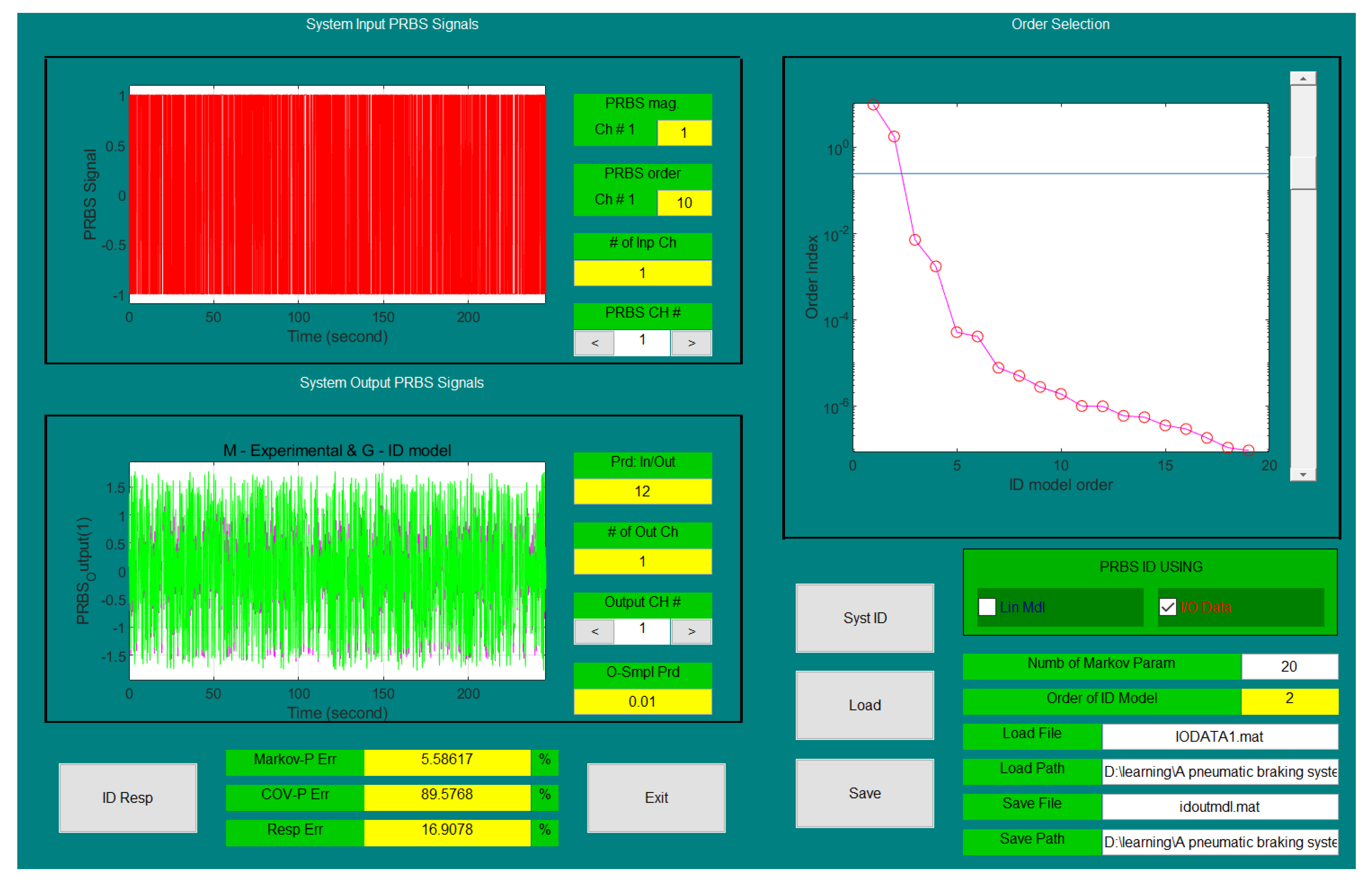
In the paper, a 10th-order inversed PRBS signal, a 0.12 s sampling period of the PRBS signal, and a 0.01 s sampling period of the output pressure were adopted. Under a 4 bar target pressure, a 5.8 bar supply pressure, and a PRBS magnitude of 0.8, the input signals and output signals were generated. Then, they were fed into the MATLAB Graphic User Interface (GUI) [27], and the nonlinear brake system was linearized for the second-order system. Then, the identification results were based on the chosen parameters, as shown in Figure 4. From Figure 4, the Markov-P error and response error were low, which showed the accuracy of the identification method.

The transfer function of the air brake system can be obtained based on the discrete-time state-space model of the closed-loop brake system. The form of the brake system transfer function did not vary with the different reference pressures. Therefore, the discrete-time transfer function of the linearized pneumatic brake system could be generated as Equation (3). The coefficients ${\theta }_1$, ${\theta }_2$, ${\theta }_3$, and ${\theta }_4$ in Equation (3) varied with the different target pressures.

$$G_P\left(z\right)=\frac{{\theta }_{1}z+{\theta }_2}{z^2+{\theta }_{3}z+{\theta }_4}$$

(3)

Then, under the given supply pressure, the plant model was established under different operational points as a function of the target pressure; see

Table 1. Parameters for the linear system identified under different target pressures.

Reference Pressure	${\mathit{\theta }}_1$	${\mathit{\theta }}_2$/${\mathit{\alpha }}_2$	${\mathit{\theta }}_3$/${\mathit{\alpha }}_1$	${\mathit{\theta }}_4$
2 bar	0.01497	0.01529	−1.923	0.9226
3 bar	0.01482	0.01585	−1.912	0.913
4 bar	0.01474	0.01851	−1.9	0.902

.

The data in Table 1 were analyzed, and the rules could be found, which were ${\theta }_1$ ≈ $-0.0078{\theta }_3$ and ${\theta }_4$ ≈ $-0.48{\theta }_3$. With this law, the formula was simplified, as shown in Equation (4).

$$G_P\left(z\right)=\frac{-0.0078{\alpha }_{1}z+{\alpha }_2}{z^2+{\alpha }_{1}z-0.48{\alpha }_1}$$

(4)

3.3. An LPV System

To design the gain-scheduled MPC controller, the LPV model was utilized as the state-space form based on the linear transfer function shown as Equation (4) through MATLAB/SIMULINK. The coefficient of the state-space model was obtained as follows.

$$\begin{array}{ccc}\hfill A& =& \left[\begin{array}{cc}-{\alpha }_1& 0.48{\alpha }_1\\ 1& 0\end{array}\right]\hfill \\ \hfill B& =& {\left[\begin{array}{cc}1& 0\end{array}\right]}^{\mathrm{T}},\hfill \\ \hfill C& =& \left[\begin{array}{cc}-0.0078{\alpha }_1& {\alpha }_2\end{array}\right]\hfill \end{array}$$

(5)

4. Gain-Scheduled Model Predictive Control for the LPV System

Based on the LPV model above, the MPC controller can be designed under different target levels. Due to the unmeasurability of the state variables, the Kalman filter was used for the estimation of the state variables. Over the entire operating conditions, the interpolation strategy was adopted in this section.

4.1. MPC Controller Design

MPC, also known as receding horizon control, solves an open-loop optimization problem based on the current state, output, and model of the system. The main goal of the MPC scheme is to predict the future manipulated variable to find a control sequence based on the minimized cost function. Only the first control action was applied to the system.

Considering the system process noise, t, and output measurement noise, l, at sample time k, the discrete-time state-space equation could be gathered together as Equation (6).

$$\begin{array}{c}\Delta x_n(k+1)=A_n\left(k\right)\Delta x_n\left(k\right)+B_n\left(k\right)\Delta u\left(k\right)+t\left(k\right)\hfill \\ \Delta y_n\left(k\right)=C_n\left(k\right)\Delta x_n\left(k\right)+l\left(k\right),\hfill \end{array}$$

(6)

where $x_n\left(k\right)$, $y_n\left(k\right)$, and $u\left(k\right)$ are the state vector, process output, and manipulated variables. $A_n\left(k\right)$, $B_n\left(k\right)$, and $C_n\left(k\right)$ are the coefficients of the process input, the measurement error, and the predicted output. Note that process noise, $t\left(k\right)$, and measurement noise, $l\left(k\right)$, were assumed to be zero mean and independent vectors, as follows:

$$E\left\{t\left(k\right)\right\}=0,W=E\left\{t\left(k\right)t^T\left(k\right)\right\};E\left\{l\left(k\right)\right\}=0,W=E\left\{l\left(k\right)l^T\left(k\right)\right\}$$

(7)

To solve the optimization problems, the cost function on predictions horizon P and control horizon M is given as follows:

$$minJ(y_m\left(k\right),\Delta U\left(k\right),M,P)=∥Y_p(k+1\left|k\right.)-{R(k+1)∥}^2+\Delta U{\left(k\right)}^T{R}_1\Delta U\left(k\right)$$

(8)

where $Y_p(k+1\left|k\right)$ is the predictive output, $R_1$ is an $M\times M$ weighting matrix for the desired closed-loop performance, $R(k+1)$ is the reference matrix, and $\Delta U\left(k\right)$ is the control increment.

According to Equation (6), based on the current state at sample time k, the predictive output at sample time $k+1$, ... $k+p$ can be derived as follows:

$$R(k+1)={{\left[\begin{array}{cccc}r(k+1)& r(k+2)& \cdots & r(k+p)\end{array}\right]}^T}_{p\times 1}$$

(9)

$${\mathrm{Y}}_p(k+1|k)={{\left[\begin{array}{cccc}{y}_c(k+1|k)& y_c(k+2|k)& \cdots & y_c(k+p|k)\end{array}\right]}^T}_{p\times 1}$$

(10)

$$\Delta U\left(k\right)={{\left[\begin{array}{cccc}\Delta u\left(k\right)& \Delta u(k+1)& \cdots & \Delta u(k+m-1)\end{array}\right]}^T}_{m\times 1}$$

(11)

The system’s predictive output sequence can be obtained through iteration. The compact matrix form is shown as Equation (12).

$$\begin{array}{c}Y=Fx\left(k_i\right)+H\Delta U\hfill \end{array}$$

(12)

where:

$$F={[C\ast A;C\ast A^2;\dots C\ast A^P]}_{p\times 1}^T$$

(13)

$$H={\left[\begin{array}{ccccc}CB& 0& 0& \cdots & 0\\ CAB& CB& 0& \cdots & 0\\ C{A}^{2}B& CAB& CB& \cdots & 0\\ ⋮& & & \cdots & \\ C{A}^{P-1}B& C{A}^{P-2}B& C{A}^{P-3}B& \cdots & C{A}^{P-M}B\end{array}\right]}_{P\times M}$$

(14)

The optimal solution for the control signal is shown as:

$$\Delta U={(H^{T}H+R_1)}^{-1}{H}^T(R-Fx\left(k_i\right))$$

(15)

Then, the first element of $\Delta U$ was taken in the system at time $k_i$.

4.2. Kalman Filter Estimation

Since the plant state variable could not be measured, the Kalman filter method was used to estimate the system state. Assuming a noisy environment, the state observer can reduce the noise effect on the measurement. The observer can be constructed as (16).

$$\begin{array}{c}\widehat{x}(k+1)=A\ast \widehat{x}\left(k\right)+B\ast \Delta u\left(k\right)+L\ast (y_m\left(k\right)-\widehat{y}\left(k\right))\hfill \\ \widehat{y}\left(k\right)=C\ast \widehat{x}\left(k\right)\hfill \end{array}$$

(16)

where L is the observer gain matrix. From Equation (16), the observer consisted of two parts: one was the original model, and the other was the correction term based on the error between the actual system output and the predicted system output.

The observer gain matrix L can be obtained as follows:

$$L=AP\left(k\right)C^T{(V+CP\left(k\right)C^T)}^{-1}$$

(17)

where the estimation error covariance matrix, $P\left(k\right)$, is calculated by the following difference Riccati equation:

$$P(k+1)=AP\left(k\right)A^T+W-LCP\left(k\right)A^T$$

(18)

The principle of MPC applied to the pneumatic brake system with the Kalman filter is shown in Figure 5.

The MPC with Kalman filter estimation was implemented online in MATLAB/Simulink following the steps below.

Step 1: Initialization. Set the prediction horizon P and control horizon M; $y_m(-1)$ = 0, $u(-1)$ = 0, $\widehat{x}(-1)$ = 0, given $A\left(k\right)$, $B\left(k\right)$, and $C\left(k\right)$ in Equation (5);

Step 2: Calculate the F matrix and the H matrix in Equations (13) and (14);

Step 3: According to the Kalman filter, calculate the observer gain L and predicted state $\widehat{x}\left(k\right)$ in Equation (17);

Step 4: Calculate the variation control input $\Delta u\left(k\right)=u\left(k\right)-u(k-1)$ in Equation (15);

Step 5: The system control input $u\left(k\right)$ is obtained;

Step 6: $k=k+1$, and return to Step 1.

4.3. Interpolated Strategy of Gain-Scheduled MPC

The single MPC controller was designed at each operating point: 2 bar, 3 bar, and 4 bar. The control range was limited, which should be extended for a wider application. The control strategy should be considered in the process of the design based on the independent MPC controller. The gain-scheduled MPC was designed with three independent MPC controllers to adjust for the entire range. When the reference pressure was less than 2 bar, the controller for 2 bar was chosen; if the given reference pressure was between 2 bar and 3 bar, the convex combination of the percentage of the difference between the reference pressure and 3 bar multiplied by the parameters for the 2 bar controller and the percentage of the difference between the reference pressure and 2 bar multiplied by the parameters for the 3 bar controller were chosen; for example, for the desired pressure of 2.6 bar, forty percent of the parameter for the 3 bar controller and $60\%$ of the parameter for the 2 bar controller were used. Similarly, for the given target pressure between 3 bar and 4 bar, the convex combination of the 3 bar controller and the 4 bar controller was used. The 4 bar controller was used for the reference pressure above 4 bar.

5. Simulation Validation

The nonlinear model and the MPC controller based on the discrete-time linear identified model were implemented in MATLAB/Simulink and validated. With the sample time of $0.001$, under different reference pressures, the control parameters—the predictive horizon P and the control horizon M—were tuned in MATLAB/Simulink. Then, in the process of the simulation, the Kalman filter gain L was obtained. The parameters under different reference levels are shown in

Table 2. Parameters for the simulation with the MPC controller under different reference pressure levels.

Reference Pressure	Predictive Horizon P	Control Horizon M	Kalman Filter Gain L
2 bar	50	10	[5.5, 4.3]
3 bar	60	12	[9.2, 7.3]
4 bar	68	14	[9.6, 8.4]

.

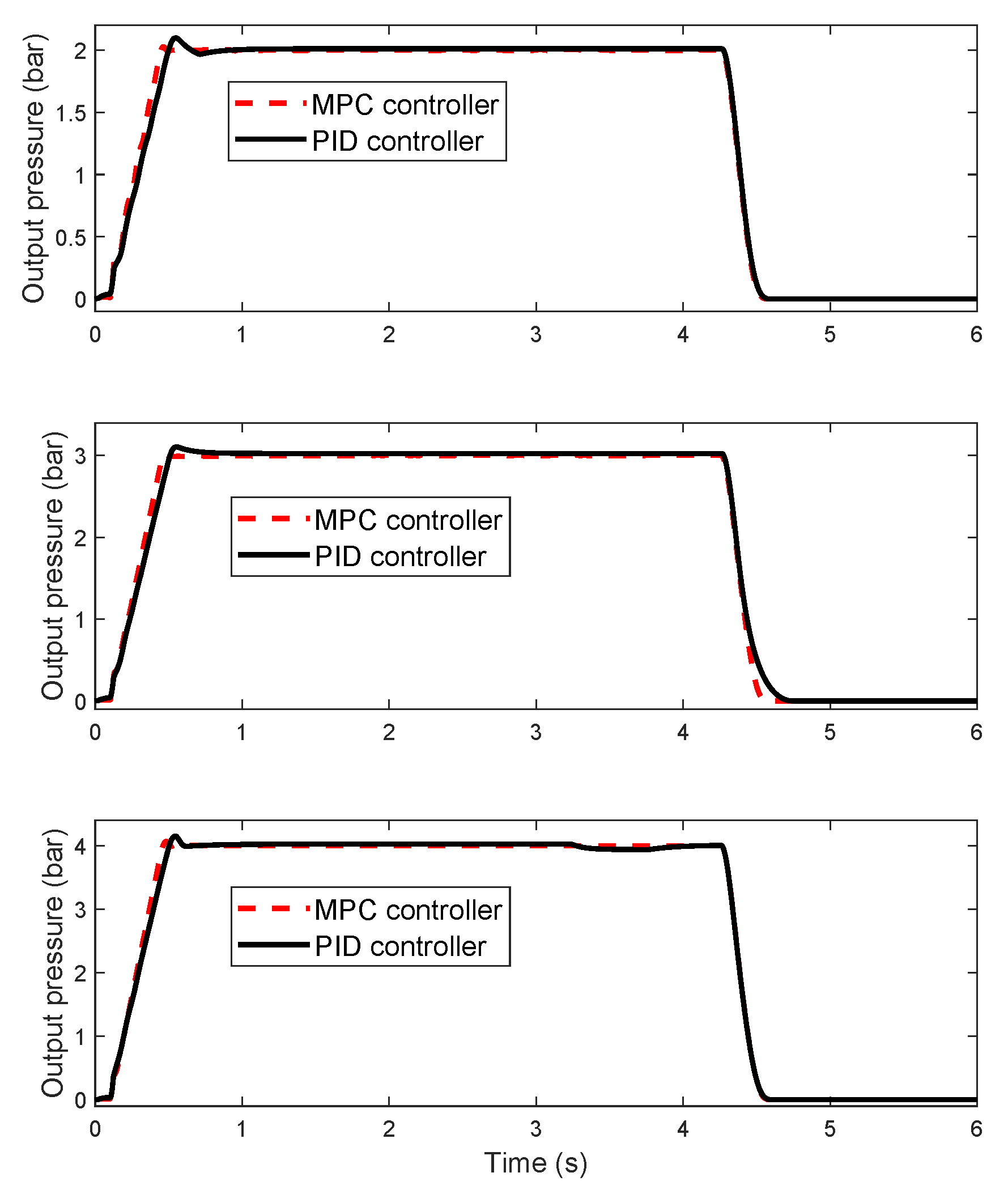
To better reflect the performance of the MPC controller, with the same step input signal for the PID controller and the MPC controller, under the target pressures of 2 bar, 3 bar, and 4 bar with the reservoir supply pressure of 5.8 bar, the results of the PID controller, which was tuned with the optimization parameters, were compared with those of MPC controller, as shown in Figure 6.

From Figure 6, the response time in the charging process and the discharging process for the PID controller was slower than that for the MPC controller. The system tracking performance with the MPC controller was better than that with the PID controller.

6. Experimental Validation

To validate the controller above, the electro-pneumatic proportional valve needed to be transformed first. The control circuit of the proportional valve was removed, and the signal of the solenoid valve was connected by the cable, which would connect to dSPACE. Figure 7 shows the proportional valve after the transformation.

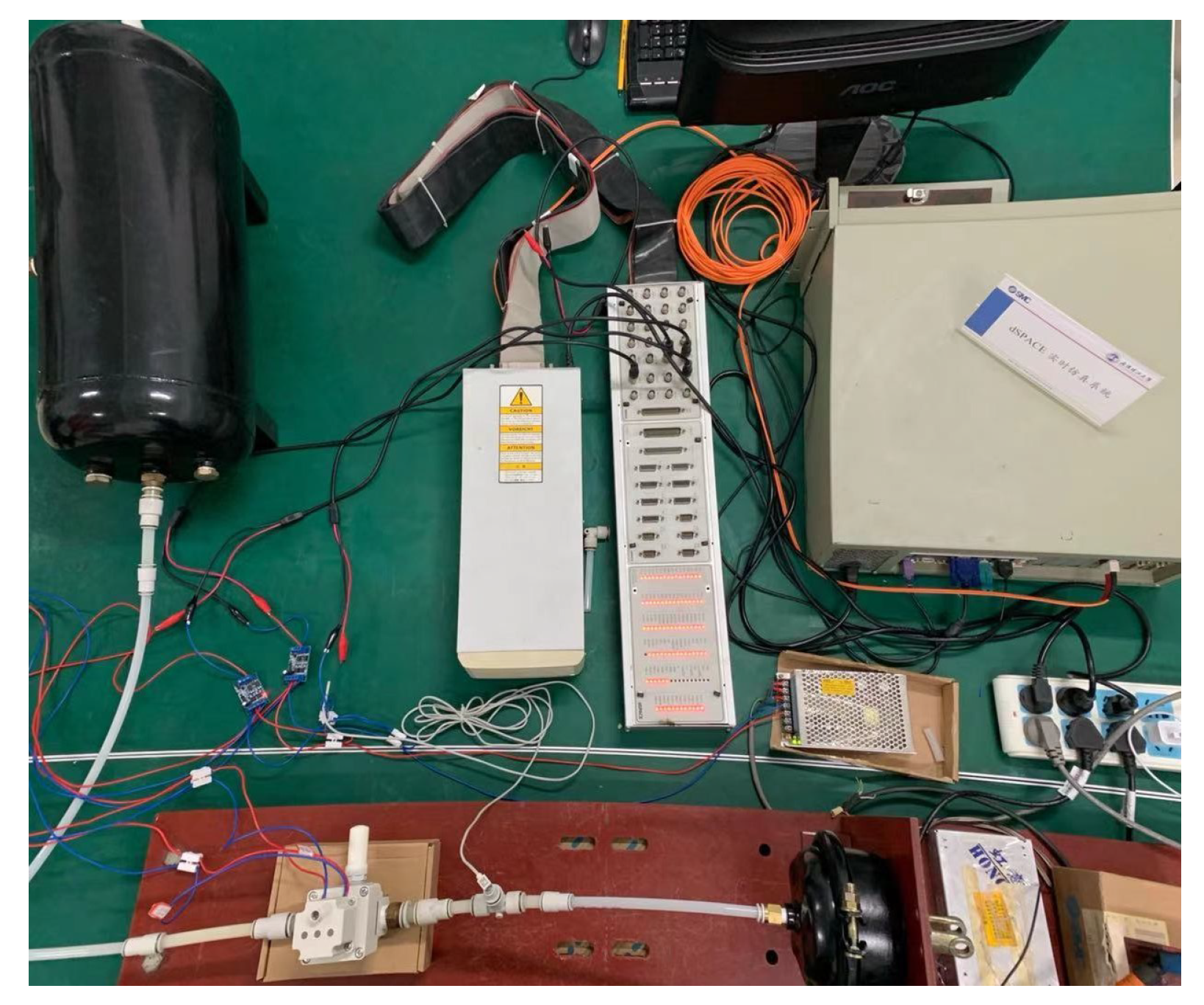
The experimental validation was conducted on the pneumatic circuit. Figure 8 shows the test bench setup, which consisted of the compressor, tank, pressure regulator, proportional valve, brake chamber, pressure sensor, and dSPACE. The gas from the compressor reached the brake chamber through the tank, pressure regulator, and proportional valve. The gas tank and the pressure regulator were used to stabilize the pressure and adjust the supply pressure, respectively. The designed MPC controller was loaded into dSPACE. Since the voltage of dSPACE was different from that of the proportional valve, the amplifier was needed and added to the circuit to match each other.

The proposed MPC controller with the Kalman filter was performed on the test bench based on dSPACE. Under the target pressures of 2 bar, 3 bar, and 4 bar with the supply pressure of 5.8 bar, the comparison results between the simulation data and the experimental data are shown in Figure 9.

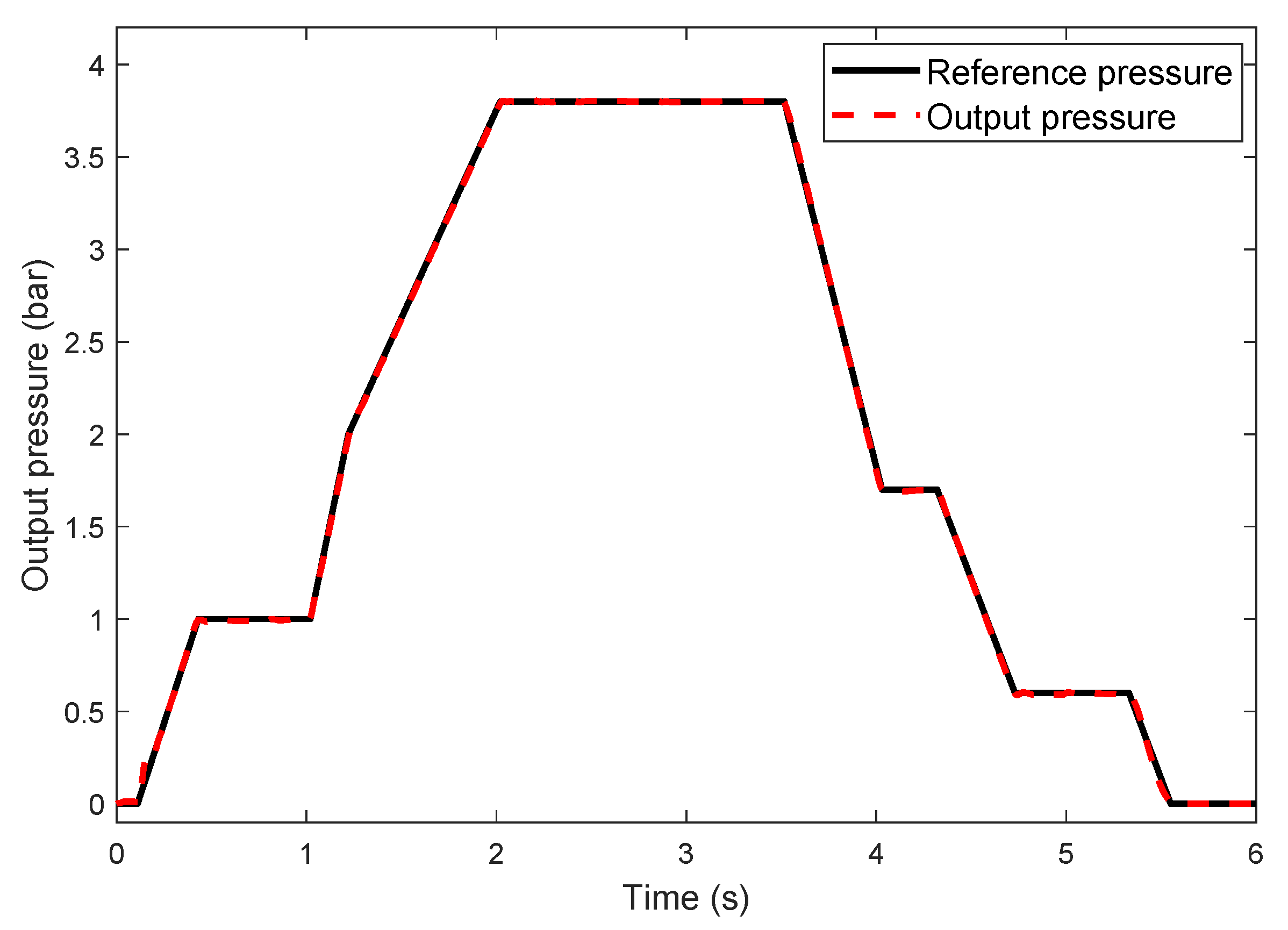
From Figure 9, the simulation data fit well with the experimental data, which verified the accuracy of the proposed MPC controller. The gain-scheduled MPC switched among a family of MPC controllers to control the nonlinear brake system based on the interpolation strategy over a wide range of target pressures. To validate the strategy, the gain-scheduled MPC was applied to this system with the complex reference signal. The results are shown in Figure 10. Figure 10 shows the tracking performance and stability of the system with a gain-scheduled MPC controller.

7. Conclusions

This paper proposed the gain-scheduled MPC controller based on the pneumatic brake system nonlinear model, a family of the linearized models at different target pressures, and the LPV model with two varying parameters for a commercial vehicle pneumatic brake system. A set of linearized models was obtained by using the q-Markov Cover system identification method. The MPC controller was designed at different target pressures, which was validated by a simulation in MATLAB/Simulink and an experiment on a test bench. Compared with the PID controller, the performance of the system with the MPC controller was better than that with the PID controller. The simulation results fit well with the experimental results. To expand the operating range of the MPC controller, the gain-scheduled MPC was designed with an interpolation strategy. With the complex reference pressure, the gain-scheduled MPC controller was validated, which showed good tracking performance and stability.

References

- Jonner, W.D.; Winner, H.; Dreilich, L.; Schunck, E. Electrohydraulic Brake System—The First Approach to Brake-By-Wire Technology. Object Detect. Collis. Warn. Avoid. Syst. 1998, 105, 1368–1375. [Google Scholar]
- Young, M.S.; Stanton, N.A. Back to the future: Brake reaction times for manual and automated vehicles. Ergonomics 2007, 50, 46–58. [Google Scholar] [CrossRef]
- Yang, W.; Zhang, X.; Lei, Q.; Cheng, X. Research on Longitudinal Active Collision Avoidance of Autonomous Emergency Braking Pedestrian System (AEB-P). Sensors 2019, 19, 4671. [Google Scholar] [CrossRef] [PubMed] [Green Version]
- Schratter, M.; Hartmann, M.; Watzenig, D. Pedestrian Collision Avoidance System for Autonomous Vehicles. SAE Int. J. Connect. Autom. Veh. 2019, 2, 279–293. [Google Scholar] [CrossRef]
- Lee, S.D.; Kim, S.L. Characterization and development of the ideal pedal force, pedal travel, and response time in the brake system for the translation of the voice of the customer to engineering specifications. Proc. Inst. Mech. Eng. Part D J. Automob. Eng. 2010, 224, 1433–1450. [Google Scholar] [CrossRef]
- Zamzamzadeh, M.; Saifizul, A.; Ramli, R.; Soong, M. Dynamic simulation of brake pedal force effect on heavy vehicle braking distance under wet road conditions. Int. J. Automot. Mech. Eng. 2016, 13, 3555–3563. [Google Scholar] [CrossRef]
- Wang, Z.; Zhou, X.; Yang, C.; Chen, Z.; Wu, X. An experimental study on hysteresis characteristics of a pneumatic braking system for a multi-axle heavy vehicle in emergency braking situations. Appl. Sci. 2017, 7, 799. [Google Scholar] [CrossRef] [Green Version]
- Palanivelu, S.; Patil, J.; Jindal, A.K. Modeling and Optimization of Pneumatic Brake System for Commercial Vehicles by Model Based Design Approach. Brake Colloquium & Exhibition 35th Annual. 2017. Available online: https://www.sae.org/publications/technical-papers/content/2017-01-2493/ (accessed on 19 May 2021).
- He, R.; Xu, C. Prediction and Control of Response Time of the Semitrailer Air Braking System. SAE Int. J. Commer. Veh. 2019, 12, 139–150. [Google Scholar] [CrossRef]
- Gautam, V.; Rajaram, V.; Subramanian, S.C. Model-based braking control of a heavy commercial road vehicle equipped with an electropneumatic brake system. Proc. Inst. Mech. Eng. Part D J. Automob. Eng. 2017, 231, 1693–1708. [Google Scholar] [CrossRef]
- Rao, S.Y.; Jeong, J.Y.; Ashby, R.M.; Heydinger, G.J.; Guenther, D.A. Modeling and Validation of ABS and RSC Control Algorithms for a 6×4 Tractor and Trailer Models using SIL Simulation. SAE 2014 World Congress & Exhibition. 2014. Available online: https://www.sae.org/publications/technical-papers/content/2014-01-0135/ (accessed on 19 May 2021).
- Zhang, J.; Sun, W.; Liu, Z.; Zeng, M. Comfort braking control for brake-by-wire vehicles. Mech. Syst. Signal Process. 2019, 133, 106255. [Google Scholar] [CrossRef]
- Riexinger, L.; Sherony, R.; Gabler, H. Has Electronic Stability Control Reduced Rollover Crashes? WCX SAE World Congress Experience. SAE Int. 2019. [Google Scholar] [CrossRef]
- Han, J.; Zong, C.; Zhao, W. Development of a Control Strategy and HIL Validation of Electronic Braking System for Commercial Vehicle. 2014. Available online: https://www.sae.org/publications/technical-papers/content/2014-01-0076/ (accessed on 19 May 2021).
- Seo, M.; Yoo, C.; Park, S.S.; Nam, K. Development of Wheel Pressure Control Algorithm for Electronic Stability Control (ESC) System of Commercial Trucks. Sensors 2018, 18, 2317. [Google Scholar] [CrossRef] [PubMed] [Green Version]
- Lin, C.; Pei, X.; Guo, X. A Comparative Study on ESC Drive and Brake Control Based on Hierarchical Structure for Four-Wheel Hub-Motor-Driven Vehicle. New Energy & Intelligent Connected Vehicle Technology Conference. 2019. Available online: https://www.sae.org/publications/technical-papers/content/2019-01-5051/ (accessed on 19 May 2021).
- Zhu, B.; Zhang, P.; Wang, Z.; Zhao, J.; Wu, J.; Feng, Y. Modeling and control of Active pneumatic braking system for tractor-semitrailer combination. Automot. Eng. 2019, 1050–1055. [Google Scholar] [CrossRef]
- Zheng, H.; Miao, Y.; Li, B. A Heavy Tractor Semi-Trailer Stability Control Strategy Based on Electronic Pneumatic Braking System HIL Test. SAE Int. J. Veh. Dyn. Stab. NVH 2019, 3, 237–249. [Google Scholar] [CrossRef]
- Cheng, S.; Li, L.; Guo, H.Q.; Chen, Z.G.; Song, P. Longitudinal Collision Avoidance and Lateral Stability Adaptive Control System Based on MPC of Autonomous Vehicles. IEEE Trans. Intell. Transp. Syst. 2019, 21, 1–10. [Google Scholar] [CrossRef]
- Zhang, W. A robust lateral tracking control strategy for autonomous driving vehicles. Mech. Syst. Signal Process. 2021, 150, 107238. [Google Scholar] [CrossRef]
- Qu, S.; He, T.; Zhu, G.G. Engine EGR Valve Modeling and Switched LPV Control Considering Nonlinear Dry Friction. IEEE Asme Trans. Mechatron. 2020, 25, 1668–1678. [Google Scholar] [CrossRef]
- He, T.; Zhu, G.G.; Swei, S.S.M. Smooth Switching LPV Dynamic Output-feedback Control. Int. J. Control. Autom. Syst. 2020, 18, 1367–1377. [Google Scholar] [CrossRef]
- Cavanini, L.; Ippoliti, G.; Camacho, E.F. Model Predictive Control for a Linear Parameter Varying Model of an UAV. J. Intell. Robot. Syst. 2021, 101. [Google Scholar] [CrossRef]
- Wang, R.; Liu, C.; Shi, Y. Optimal control of aero-engine systems based on a switched LPV model. Asian J. Control. 2021. [Google Scholar] [CrossRef]
- Stewart, H.L.; Philbin, T. Pneumatics and Hydraulics; T. Audel: Springfield, MA, USA, 1976. [Google Scholar]
- Hu, D.; Li, G.; Zhu, G.; Liu, Z.; Wang, Y. A Control-Oriented LPV Model for a Commercial Vehicle Air Brake System. Appl. Sci. 2020, 10, 4589. [Google Scholar] [CrossRef]
- Zhu, G.G.; Skelton, R.E.; Li, P. Q-Markov Cover identification using pseudo-random binary signals. Int. J. Control 1995, 62, 1273–1290. [Google Scholar] [CrossRef]
Figure 1.
The simplified pneumatic brake system scheme.
Figure 2.
The sketch of the electro-pneumatic proportional valve (Reproduced with permission from [Dawei Hu], [Applied sciences]; published by [MDPI], [2020].)
Figure 3.
Closed-loop control system with the MPC controller framework.
Figure 4.
The identification results based on the chosen parameters.
Figure 5.
The principle of MPC applied to the system.
Figure 6.
Comparison results between the PID controller and the MPC controller.
Figure 7.
The proportional valve after the transformation. (a) The front part of the valve; (b) the rear part of the valve.
Figure 8.
Test bench setup.
Figure 9.
Comparison results between the simulation data and experimental data.
Figure 10.
Comparison results between the reference pressure and the output pressure with the gain-scheduled MPC controller.