FPGA-Based Implementation of an Optimization Algorithm to Maximize the Productivity of a Microbial Electrolysis Cell

Abstract

In this work, the design of the hardware architecture to implement an algorithm for optimizing the Hydrogen Productivity Rate (HPR) in a Microbial Electrolysis Cell (MEC) is presented. The HPR in the MEC is maximized by the golden section search algorithm in conjunction with a super-twisting controller. The development of the digital architecture in the implementation step of the optimization algorithm was developed in the Very High Description Language (VHDL) and synthesized in a Field Programmable Gate Array (FPGA). Numerical simulations demonstrated the feasibility of the proposed optimization strategy embedded in an FPGA Cyclone II. Results showed that only $21\%$ of the total logic elements, $5.19\%$ of dedicated logic registers, and $64\%$ of the total eight-bits multipliers of the FPGA were used. On the other hand, the estimated power consumption required by the FPGA-embedded optimization algorithm was only 146 mW.

1. Introduction

Nowadays, biotechnological systems represent a very attractive option for hydrogen production. The degradation of organic matter through the use of bacteria has gained great interest in the scientific community because hydrogen can be produced in a clean way [1,2]. In contrast to current industrial methods, in which unfortunately $90\%$ of the hydrogen produced requires the use of fossil fuels generating a large amount of $C{O}_2$ (10 tonnes of $C{O}_2$ per ton of $H_2$) [3], Microbial Electrolysis Cells (MEC) represent a great alternative to produce hydrogen because they require less energy compared to the classic techniques to produce hydrogen, such as the electrolysis of water [4,5].

A MEC is an electrochemical device which uses electroactive microorganisms as catalysts to convert the organic matter to hydrogen and provides a novel approach for producing economically viable hydrogen from a wide range of renewable biomass sources [6,7]. Furthermore, a waste biorefinery based on MECs to produce clean and renewable electrofuel and valuable chemical compounds holds the flexible potentials for pollutants removal and $C{O}_2$ capture [8]. Broadly speaking, unlike a Microbial Fuel Cell, a MEC requires the induction of a constant voltage supply generating a potential difference between the electrodes to produce a flow of hydrogen as a result of the degradation of the organic matter that is fed to the MEC.

Other widely biological approaches used for the production of hydrogen in a clean way include Dark Fermentation (DF) in which bioreactors are fed by wastewater with a high concentration of organic matter from domestic and industrial origin. However, its efficiency to produce hydrogen compared to a MEC is relatively low (40% or less) [9]. Generally a MEC is fed with a controlled flow of wastewater which is rich in Volatile Fatty Acids (VFAs) that in turn might come from another Wastewater Treatment Plant (WWTP) like a DF bioreactor.

The production of hydrogen at the industrial scale through biotechnological systems is a challenge that has been dealt with from different approaches. For instance, in [10] an optimization scheme to maximize the hydrogen productivity of a DF is presented. In such study the optimization is achieved by a heuristic strategy with a nonlinear observer consisting in a Luenberger observer coupled to a super-twisting observer. Then, a super-twisting controller is used to lead the DF process to its maximum hydrogen productivity rate. In [11] the optimization is focused on the effect of the operating conditions such as pH, temperature, nutrient availability and substrate concentration. This involves mathematical modeling of a fermentation process in such a way that biohydrogen production can be predicted. On the other hand in [12] the hydrogen productivity was reported to increase from 0.13 to 0.82 m³ $\left[H_2\right]$ per m³ per day improving the conductivity of the electrode in a MEC and increasing the population of bacteria in the cathode biofilm. Another work related to hydrogen optimization is presented in [13] where the authors demonstrated that the MEC efficiency can be improved through the reduction of the apparent resistance. The optimization strategy is integrated by both perturbation and observation algorithms designed to track the minimal apparent resistance and adjusting the applied voltage used as control input. Other works in literature are focused in MEC construction details, for example, in [14] an effective strategy to improve the productivity performance through an improved anode arrangement is presented. In such work, the anode is strategically located in such a way that the solution resistance, the biofilm and the whole physical system are reduced. The polarization of the MEC was considerably reduced, affecting directly 72–118% the rate of hydrogen production.

The possibility of being able to implement control algorithms using digital systems such as microcontrollers, Graphic Processing Units (GPUs) and Field Programmable Gate Arrays (FPGAs) has been of great interest due to its great processing capacity, resources optimization and low energy consumption. Besides, the parallelism in the execution of the algorithms has given to the FPGAs a great advantage over other digital systems based on microcontrollers and microprocessors. For example, in [15,16], an FPGA-based fuzzy-logic controller is implemented and analyzed, and it is concluded that this technology is a good choice for implementation. The parallelism offered by FPGAs is used in [17,18] to implement complex control algorithms for a AC-DC converter and a DC-DC converter, respectively. In these works the FPGA processing efficiency is highlighted. In [19] both, the optimization of 80% of the hardware and reduction of 40% of the power consumption of a distributed-arithmetic (DA)-based proportional-integral-derivative (PID) controller compared to a multiplier-based scheme is demonstrated for temperature control. The efficiency of the complete digital control system is demonstrated using a Xilinx Spartan-2E FPGA. More recently, in [20] the authors proposed a combination of a direct torque control, space vector modulation, input-output feedback linearisation, a second-order super-twisting speed controller, and sliding-mode-load torque and stator-flux observers with stator resistance estimation implemented in an FPGA. This control strategy demonstrated robustness in presence of stator resistance variations and uncertainties when it was applied to an induction motor drive. An interesting pipeline implementation of a super-twisting controller to control ground vehicles is presented in [21]. The super-twisting controller was used to control the lateral and yaw velocities in the vehicle dynamics that are described by a discrete time model. The resulting implementation required shorter sampling times and can be synthesized in a low-cost FPGA. A classical Proportional-Integral-Derivative (PID) controller implemented in FPGA is proposed in [22]. With the objective to accelerate the execution of the algorithm, to obtain great precision and to get highly commercial ability, the implementation was based on smooth motion interpolation. The results from numerical simulations and practical tests, demonstrated its correct performance. Nevertheless, to the best of the authors knowledge, there is not FPGA-based control implementations applied to bioprocesses.

In the present work the optimization problem of maximizing the Hydrogen Production Rate (HPR) in a MEC is addressed. The productivity function is approximated from the MEC model in steady state, for which, a point of maximum performance in a well-defined operating region is ensured. Using the golden section search optimization algorithm coupled to a robust super-twisting controller, the MEC is online brought to its maximum hydrogen production performance. The proposed optimization strategy is embedded in an FPGA throughout different digital architectures that are executed in parallel without hardware sharing. The resulting digital architecture has mainly two advantages, first, the portability to be synthesized in an FPGA card from any manufacturer, and second, the low power consumption compared to a personal computer. The implementation of the optimization algorithm in an FPGA has the great advantage of being described in hardware. This allows an easy adaptation in the use of communication protocols with external devices.

The rest of the paper is organized as follows: in Section 2 the mathematical model of the MEC is described, and the objective function as the HPR is presented. A description of the optimization problem is described in detail in Section 3. In Section 4 the optimization problem is addressed by using the Golden Section Search algorithm coupled to the discrete time super-twisting controller. In addition, the maximum HPR numerically computed is verified analytically. The FPGA-based implementation of the optimization algorithm is presented in Section 5 including numerical algorithms for the implementation of arithmetic operations like division, multiplication and square root. The results are presented in Section 6, where numerical simulations are carried out in an FPGA to verify the performance, including both the truncation error and the synthesis report of the digital architecture. Finally some conclusions are pointed out in Section 7.

2. Mathematical Model

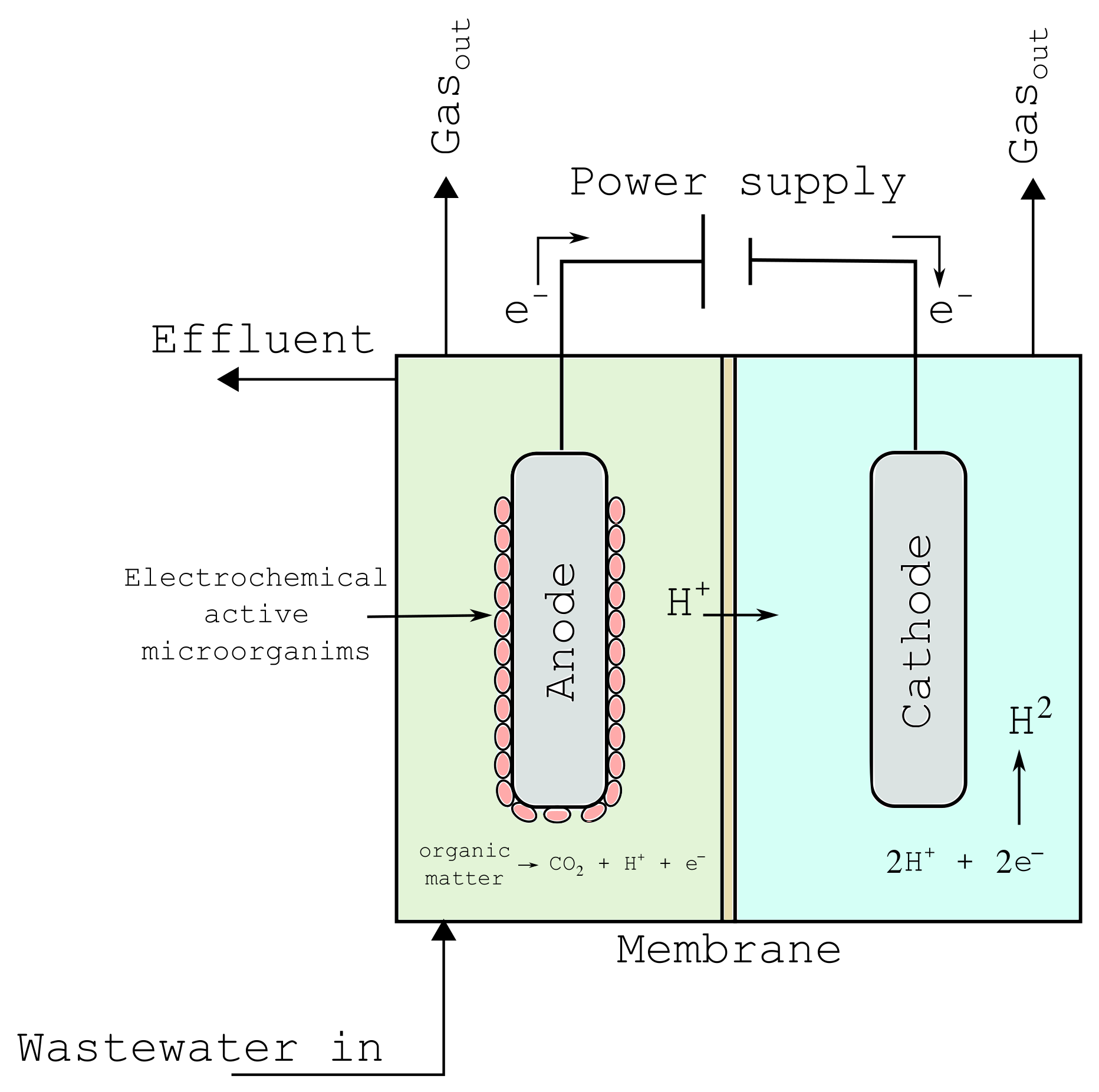
One of the most used Microbial Electrolysis Cell (MEC) configurations currently consists mainly of two chambers that are separated by a cathode membrane (see Figure 1). In the anode chamber, the anode is covered by a biofilm where the existence of anodophilic and methanogenic bacteria is considered. The degradation of VFAs in the MEC takes place in the anode chamber, where hydrogen protons and electrons are produced. Protons pass through a ionic membrane to the cathodic chamber where the production of hydrogen occurs. A relatively small voltage is supplied to the system generating a potential difference between the two electrodes, which allows the electrons released in the anode by the anodophilic bacteria to circulate and pass to the cathode to combine with the hydrogen protons. In the degradation process there is a competition between two types of microorganisms, anodophilic and methanogenic, to decide who will consume the substrate.

This behavior is modeled by the following system of Ordinary Differential Equations (ODEs) [23]:

$$\dot{s}=(s_{in}-s)D_{in}-k_a{\mu }_a{x}_a-k_m{\mu }_m{x}_m$$

(1)

$${\dot{x}}_a={\mu }_a{x}_a-k_{d,a}{x}_a-{\alpha }_a{D}_{in}{x}_a$$

(2)

$${\dot{x}}_m={\mu }_m{x}_m-k_{d,m}{x}_m-{\alpha }_m{D}_{in}{x}_m,$$

(3)

where s is the acetate concentration (mg/L⁻¹), while $x_a$ and $x_m$ are the concentration of the anodophilic and acetoclastic methanogenic microorganisms, respectively (mg/L⁻¹); $D_{in}$ is the dilution rate, $D_{in}=F_{in}/V_{reac}$ (d⁻¹), where $F_{in}$ is the input flow rate (Ld⁻¹) and $V_{reac}$ is the reactor volume (L); ${\alpha }_a$ and ${\alpha }_m$ are the dimensionless biofilm retention constants. ${\mu }_a$ and ${\mu }_m$ are the growth rates (d⁻¹) for anodophilic and acetoclastic methanogenic microorganisms, respectively, which are defined as follows:

$${\mu }_a={\mu }_{max,a}\frac{s}{k_{s,a}+s}\frac{1}{1+e^{-\frac{F}{RT}\eta }}$$

(4)

$${\mu }_m={\mu }_{max,m}\frac{s}{k_{s,m}+s},$$

(5)

where ${\mu }_{max,a}$ and ${\mu }_{max,m}$ are the maximum grown rates (d⁻¹), $k_{s,a}$ and $k_{s,m}$ are the half-rate Monod constants (mg (s) L⁻¹), F is the Faraday constant (C mol⁻¹ e⁻¹), R is the ideal gas constant (J mol⁻¹ K⁻¹), T is the temperature (K), $\eta =E_{anode}-E_{Ka}$ is the local potential, where $E_{anode}$ is the anode potential (V) and $E_{Ka}$ is the half-maximum-rate anodic Electron Aceptor (EA) potential (V) i.e., the potential that occurs when $S=k_{S,a}$ and the rate is half of the maximum rate [24].

MEC Productivity

The hydrogen flow rate in the MEC is modeled by Equation (6), where it can be seen that the hydrogen produced is closely related to the current generated from the flow of electrons between the electrodes.

$$Q_{H2}=Y_{H2}{A}_a\frac{I_{MEC}}{mF}\frac{RT}{P},$$

(6)

where $Y_{H2}$ is the dimensionless cathode efficiency, $A_a$ is the anode area (m²), m is the electrons per mol specie (mol e⁻ mol⁻¹ M⁻¹) and P is the pressure inside the cathodic chamber (atm). In the Equation (6) the methanogenic microorganisms consumption is neglected and it is considered that only anodophilic microorganisms are responsible for acetate degradation. The current in the MEC is modeled as:

$$I_{MEC}=\left({\gamma }_s{k}_a{\mu }_a{x}_a{L}_f(1-f_s^0)+{\gamma }_{x}b{x}_a{L}_f\right)A_a,$$

(7)

where ${\gamma }_s$ and ${\gamma }_x$ (mFM⁻¹ ${\mathrm{W}}_{\mathrm{s}}^{-1}$) are the yield coefficients related to the number of coulombs that it is possible to obtain from $W_s$ (g mol⁻¹) and $W_x$ (g mol⁻¹), i.e., the substrate, and the biomass respectively; $f_s^0$ is the dimensionless fraction of electrons used for cell synthesis, b is the endogenous decay coefficient (d⁻¹) and $L_f$ is the biofilm thickness (m).

The hydrogen production rate (HPR) $Q_{H_{2,p}}$ is defined as the hydrogen flow rate produced per volume of reactor ($L\left[H_2\right] {\mathrm{L}}^{-1}{\mathrm{d}}^{-1}$):

$$Q_{H_{2,p}}=\frac{Q_{H_2}}{V_{reac}},$$

(8)

where $Q_{H_2}$ is the hydrogen flow rate defined by Equation (6).

3. Problem Statement

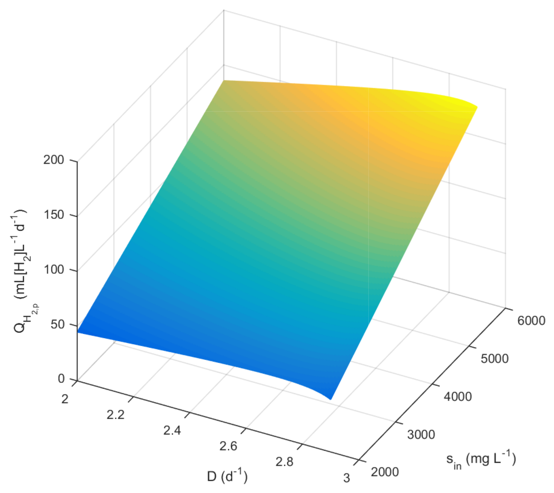
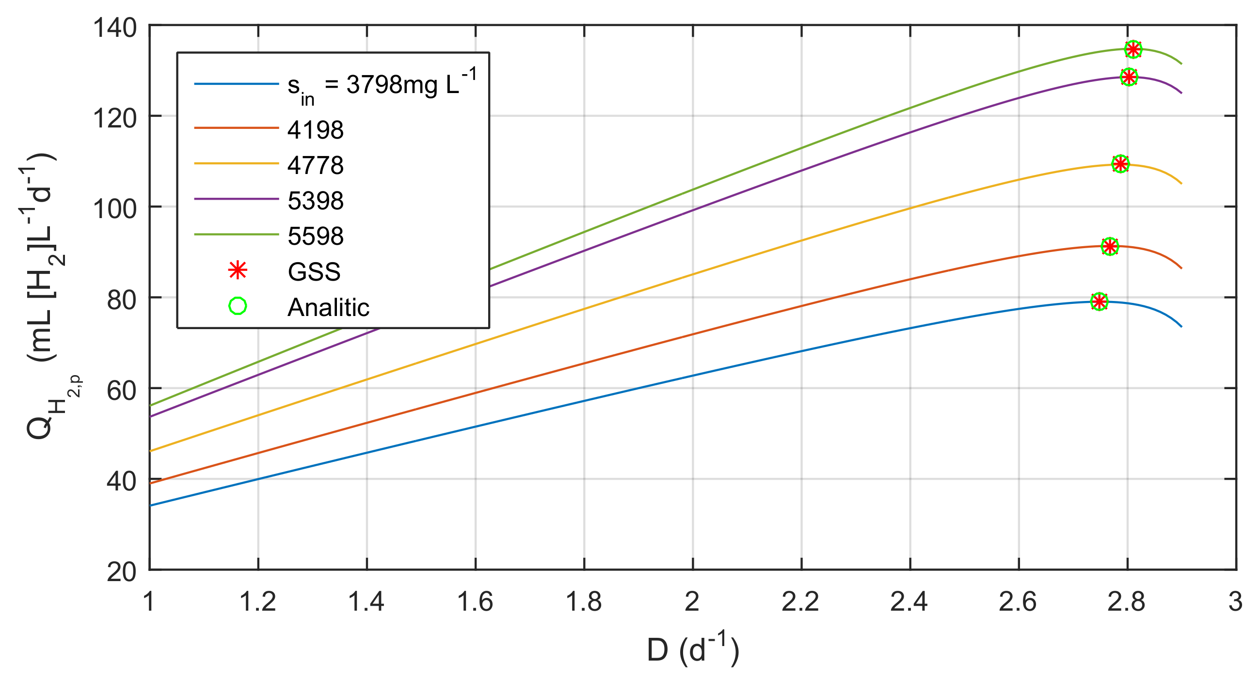
The HPR is function of both, the dilution rate $D_{in}$ and the inlet acetate concentration $s_{in}$. $D_{in}$ is the optimization variable, while $s_{in}$ is considered as a disturbance. As it can be seen in Figure 2, the HPR presents a maximum hydrogen productivity point related to an optimal dilution rate ($Q_{H_{2,p}max},D_{in,opt}$) within a range of concentrations for the inlet acetate $s_{in}$ [2000, 6000] mL⁻¹. Therefore, the optimization problem consists in calculating the value of the optimal dilution rate $D_{in,opt}$ that ensures the maximum performance $Q_{H_{2,p}max}$ in the MEC.

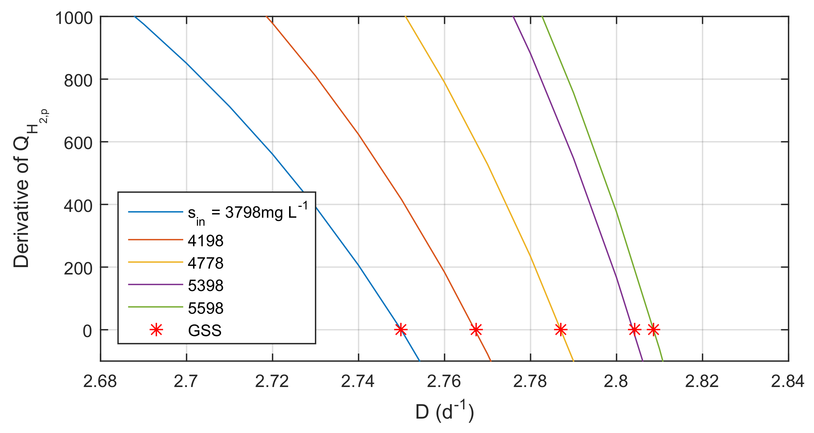
Maximizing the HPR in the MEC is possible if and only if a $D_{in,opt}$ of the productivity function $Q_{H_{2,p}}(D_{in},s_{in})$ can be computed in an open neighborhood region ($\Gamma$) for each acetate concentration in the inlet $s_{in}$. Ensuring the existence of $D_{in,opt}$ implies the following assumptions [25]:

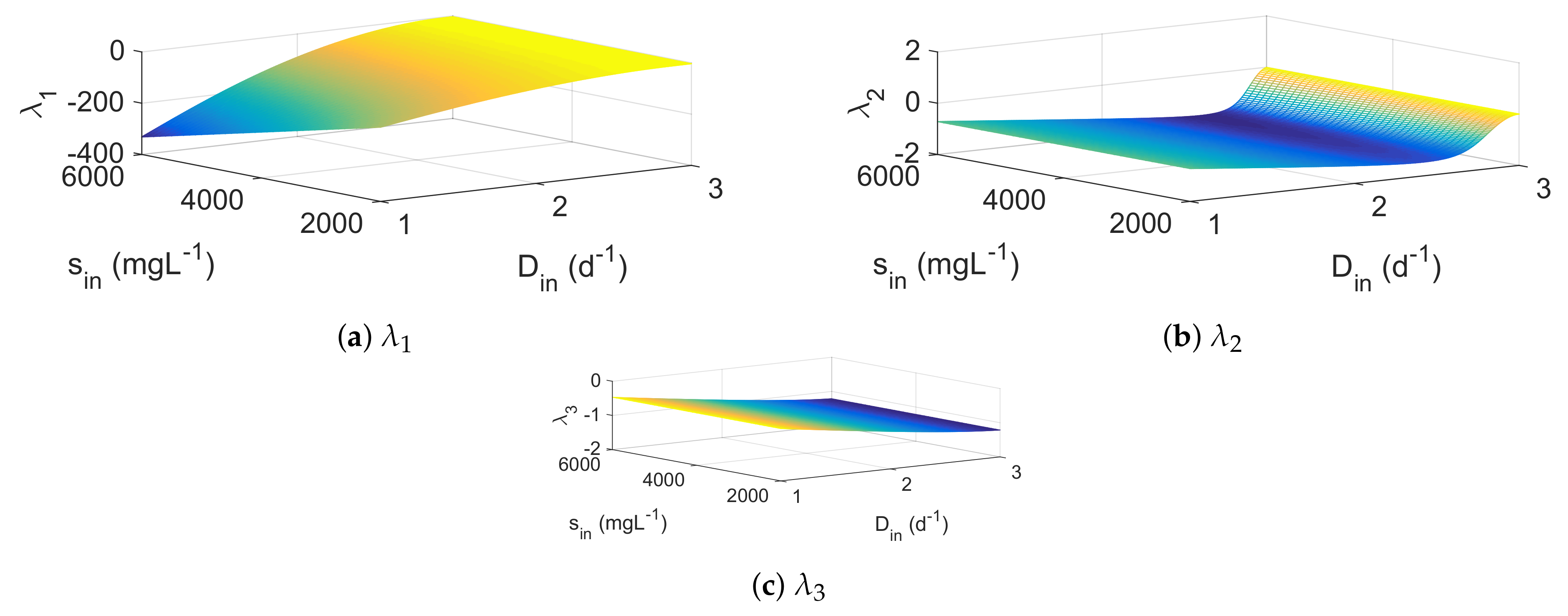
Assumption 1.

The function $Q_{H_{2,p}}$ is twice continuously differentiable in Γ with respect to $D_{in}$ such that:

$$\begin{array}{c}\frac{\partial Q_{H_{2,P}}(D_{in,opt},s_{in})}{\partial D_{in}}=0\\ \frac{{\partial }^2{Q}_{H_{2,P}}(D_{in},s_{in})}{\partial D_{in}^2}<0\end{array}$$

(9)

Assumption 2.

The function $Q_{H_{2,p}}$ is convex, unimodal and any $D_{in,opt}$ is a global maximizer for each $s_{in}$ in the operating region.

The optimization problem to maximize the hydrogen production rate in the MEC is proposed as:

$$\begin{array}{c}\underset{D_{in}}{max} Q_{H_{2,p}}(D_{in},s_{in})\hfill \\ \mathrm{such} \mathrm{that}:\hfill \\ \begin{array}{ccc}\dot{x}\left(t\right)& =& f(x,D_{in},s_{in})\\ y\left(t\right)& =& Q_{H_{2,p}}\left(x\right),\end{array}\hfill \end{array}$$

(10)

where $x={[s,x_a,x_m]}^T$ is the state vector, $f(x,D_{in},s_{in})$ is defined by Equations (1)–(5) and the measured output $Q_{H_{2,p}}\left(x\right)$ is the hydrogen production rate defined by Equations (6)–(8).

As it is shown in Figure 2, only a maximum $Q_{H_{2,p}max}$ can be observed for each maximizer $D_{in,opt}$ in the operating region.

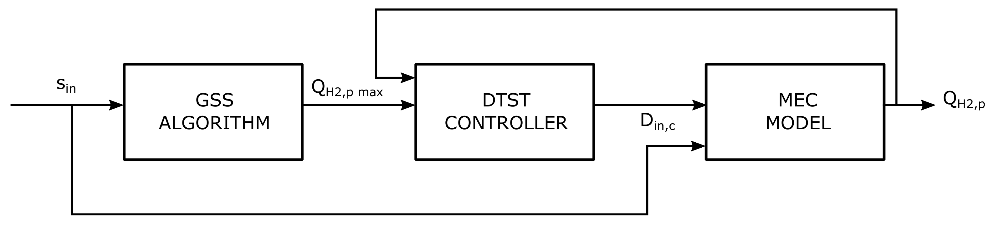
The optimization problem is online solved by the GSS algorithm coupled to a super-twisting controller. The GSS algorithm calculates the value $Q_{H_{2,p}max}$ using a hydrogen productivity function in relation to both, the dilution rate and the inlet acetate concentration of the MEC. The super-twisting controller uses $Q_{H_{2,p}max}$ as a reference to track the MEC productivity to the maximum value. The optimization scheme described before is depicted in Figure 3.

In order to optimize the hardware resources and to reduce the power consumption, the optimization strategy to maximize the HPR of the MEC is embedded in an FPGA. This way, the energy cost required to bring the MEC to its maximum HPR can be considerably reduced.

4. Optimization of the MEC Productivity

An optimum point ($Q_{H_{2,p}max}$, $D_{in,opt}$) is possible if and only if the MEC achieves an steady state $[s^{*},x_a^{*},x_m^{*}]$. The operating point of the system (1)–(3) as function of $s_{in}$ and $D_{in}$ is given in steady state as:

$$s^{*}=\frac{k_{s,a}{k}_{d,a}+k_{s,a}{\alpha }_a{D}_{in}}{\frac{{\mu }_{max,a}}{\psi }-k_{d,a}-D_{in}{\alpha }_a}$$

(11)

$$x_a^{*}=\frac{(s_{in}-s^{*})D_{in}}{k_a{\mu }_a}$$

(12)

$$x_m^{*}=0,$$

(13)

with

$$\psi =1+e^{-\frac{F}{RT}\eta }.$$

(14)

The objective function $Q_{H_{2,p}}(D_{in},s_{in})$, defining the input-output map in steady state, is therefore expressed as:

$$Q_{H_{2,p}}(D_{in},s_{in})=\frac{L_f{A}_{sur}{Y}_{H_2}{A}_{a}RT{D}_{in}}{mFP{V}_{reac}}(s_{in}-s^{*})\left[{\gamma }_s(1-f_s^0)+\frac{{\gamma }_{x}b\psi (k_{sa}+s^{*})}{k_a{\mu }_{max,a}{s}^{*}}\right].$$

(15)

In this work, the acetate concentration in the inlet $s_{in}$ is assumed as known.

4.1. The Golden Section Search Algorithm

Golden ratio ($\phi$) has been of a great interest to mathematicians, physicists, philosophers and artists. In antiquity, civilizations like Egyptians used the $\phi$ number as the main criterion for the construction of the Great Pyramids. The Parthenon in Greece was also built based on $\phi$ [26].

In relation to nature, the golden ratio is considered a natural constant that sets the standard in reproduction, growth patterns of living beings such as plants and animals. Their geometric relationship is described in Figure 4, where a line A–C is divided into two segments l and r by a point B where l is greater than r such that the ratio $l/r$ is equal to the ratio $(l+r)/l$.

The Golden Section Search (GSS) algorithm is an iterative process suggested to optimize one-dimensional, unimodal and well behaved functions [27], taking into account that the optimum value must be into a search region defined by a lower bound (A) and an upper bound (C), as described in Figure 4.

$$\phi =\frac{l}{r}=\frac{l+r}{l}=1.618033988\dots$$

(16)

The optimization of the HPR in the MEC begins defining the search region of Equation (15). In this case, the search region is defined by $D_{in,A}=1$ d⁻¹ and $D_{in,C}=3$ d⁻¹. Then, two inner evaluation points $D_{in,1}$ and $D_{in,2}$ are selected as function of $\phi$.

$$D_{in,1}=D_{in,A}+d$$

(17)

$$D_{in,2}=D_{in,C}-d,$$

(18)

with

$$d=(\phi -1)(D_{in,A}-D_{in,C}).$$

(19)

The error used by the GSS algorithm to stop its operation is defined as:

$$err=(\phi -1)\left|\frac{D_{in,C}-D_{in,A}}{D_{in,opt}}\right|.$$

(20)

The complete GSS algorithm to calculate the optimum point $(D_{in,opt},Q_{H_{2,p}max})$ is presented in Algorithm 1.

4.2. GSS Validation

First, let us analyze the stability of the nonlinear system (1)–(3) by calculating the eigenvalues (${\lambda }_i$) of its linear approximation. The indirect Lyapunov method establish conditions that allow us to obtain conclusions about the stability of the nonlinear system in an operating point.

Consider the nonlinear system (1)–(3) with the operating point $x^{*}=\left[s^{*}, x_a^{*}, x_m^{*}\right]$ that has the following linear approximation

$$\dot{\overline{x}}=A\overline{x}+B_u\overline{u}+B_w\overline{w},$$

(21)

where $\overline{x}=x-x^{*}$, A, $B_u$ and $B_w$ are the Jacobian matrices of the system, $\overline{u}=D_{in}-D_{in}^{*}$ and $\overline{w}=s_{in}-s_{in}^{*}$ respectively.

The indirect Lyapunov method states that the nonlinear system (1)–(3) is asymptotically stable if and only if $Re\left({\lambda }_i\right)<0$ of the matrix A, $\forall {\lambda }_i$, $i=1,2,3$, defined as:

$$A=\frac{\partial f(x,D_{in},s_{in})}{\partial x}{|}_{(x^{*},D_{in}^{*},s_{in}^{*})}.$$

(22)

As it can be seen in Figure 5 the eigenvalues of the matrix A are Hurwitz in the operating region of the MEC. It must be pointed out that the closer the dilution rate is to the value 3 d⁻¹, the more the eigenvalues ${\lambda }_1$ and ${\lambda }_2$ approach the origin.

Algorithm 1: GSS algorithm description

The optimum value $D_{in,opt}$ is then obtained by differentiating the objective function (15) with respect to $D_{in}$ and equating the result to zero (first-order optimally condition), which leads to

$$\frac{\partial Q_{H_{2,p}}}{\partial D_{in}}=\left(\frac{Y_{H2}{A}_{a}RT}{mFP{V}_{reac}}\right)\frac{\partial I_{MEC}^{*}}{\partial D_{in}}=0,$$

(23)

where

$$\begin{array}{c}\hfill \frac{\partial I_{MEC}^{*}}{\partial D_{in}}=L_f{A}_{sur}[D_{in}(s_{in}-s^{*})\left(\frac{\psi {\gamma }_{x}b}{k_a{\mu }_{max,a}}\frac{\partial \rho }{\partial D_{in}}\right)+({\gamma }_s(1-f_s^0)+\\ \hfill \frac{{\gamma }_{x}b}{k_a{\mu }_a}\left)(s_{in}-s^{*}-D_{in}\frac{\partial s^{*}}{\partial D_{in}})\right]\end{array}$$

(24)

$$\frac{\partial \rho }{\partial D_{in}}=\frac{\frac{\partial s^{*}}{\partial D_{in}}(s^{*}-(k_{sa}+s^{*}))}{{s^{*}}^2}$$

(25)

$$\frac{\partial s^{*}}{\partial D_{in}}=\frac{k_{sa}{\alpha }_a\left(\frac{{\mu }_{max,a}}{\psi }-k_{d,a}-D_{in}{\alpha }_a\right)+{\alpha }_a(k_{s,a}{k}_{d,a}+k_{s,a}{\alpha }_a{D}_{in})}{{\left(\frac{{\mu }_{max,a}}{\psi }-k_{d,a}-D_{in}{\alpha }_a\right)}^2}$$

(26)

Figure 6 shows the $Q_{H_{2,p}max}$ value calculated both, by the GSS Algorithm 1 and by substituting $D_{in,opt}$, calculated by setting the Equation (23) equal to zero (see Figure 7), in Equation (15). As it can be seen, the results of the GSS algorithm match the results obtained analytically.

4.3. Super-Twisting Controller

The MEC model (1)–(3) can be rewritten as follows:

$$\dot{x}=\gamma \left(x\right)+g\left(x\right)D_{in}$$

(27)

$$y=Q_{H_{2,p}}\left(x\right),$$

(28)

where $\gamma \left(x\right)$ and $g\left(x\right)$ are vector functions defined as:

$$\gamma \left(x\right)=\left(\begin{array}{c}-k_a{\mu }_a{x}_a-k_m{\mu }_m{x}_m\\ ({\mu }_a-k_{d,a})x_a\\ ({\mu }_m-k_{d,m})x_m\end{array}\right)$$

(29)

$$g\left(x\right)=\left(\begin{array}{c}{s}_{in}-s\\ -{\alpha }_a{x}_a\\ -{\alpha }_m{x}_m\end{array}\right).$$

(30)

The relative degree $\sigma$ of System (27) and (28) is computed by differentiating the output with respect to time as [28]:

$$\dot{y}=\frac{\partial Q_{H_{2,p}}\left(x\right)}{\partial x}\dot{x} = \beta \gamma \left(x\right)+\beta g\left(x\right)D_{in},$$

(31)

where $\beta =\left[\frac{\partial Q_{H_{2,p}}}{\partial s}, \frac{\partial Q_{H_{2,p}}}{\partial x_a}, \frac{\partial Q_{H_{2,p}}}{\partial x_m}\right]$. Hence, the relative degree of the system (27) and (28) is $\sigma =1$.

In this work the super-twisting controller, Equations (32) and (33), is therefore considered to track the maximum hydrogen flow rate computed by the GSS algorithm with the sliding variable defined as the tracking error [29].

$$D_{in,c}=-{\rho }_1\sqrt{|{ϵ}_c|}sign\left({ϵ}_c\right)+D_{nom}$$

(32)

$$\frac{d{D}_{nom}}{dt}=-{\rho }_{2}sign\left({ϵ}_c\right)$$

(33)

In the super-twisting controller (32) and (33), the tracking error is defined as:

$${ϵ}_c=Q_{H_{2,p}max}-Q_{H_{2,p}},$$

(34)

${\rho }_1$ and ${\rho }_2$ are the controller gains that ensure the finite-time stability of the tracking error, while $D_{in,c}$ is the control input necessary to bring the MEC to the maximum value $Q_{H_{2,p}max}$.

For implementation purposes in an FPGA, the discrete time super-twisting controller (DTSTC) is considered. The representative numerical solution showed in the Equations (35) and (36) is obtained from Equations (32) and (33) using the Euler’s method. The controller uses the value $Q_{H_{2,p}max}$ as a reference to carry the real productivity to its maximum value in finite time.

$$D_{in,c}\left[k\right]=-{\rho }_1\sqrt{|{ϵ}_c|}sign\left({ϵ}_c\right)+D_{nom}\left[k\right]$$

(35)

$$D_{nom}[k+1]=D_{nom}\left[k\right]-\tau {\rho }_{2}sign\left({ϵ}_c\right),$$

(36)

In Equation (36), $\tau$ (d) is the sampling time considered.

5. FPGA-Embedded Optimization Algorithm

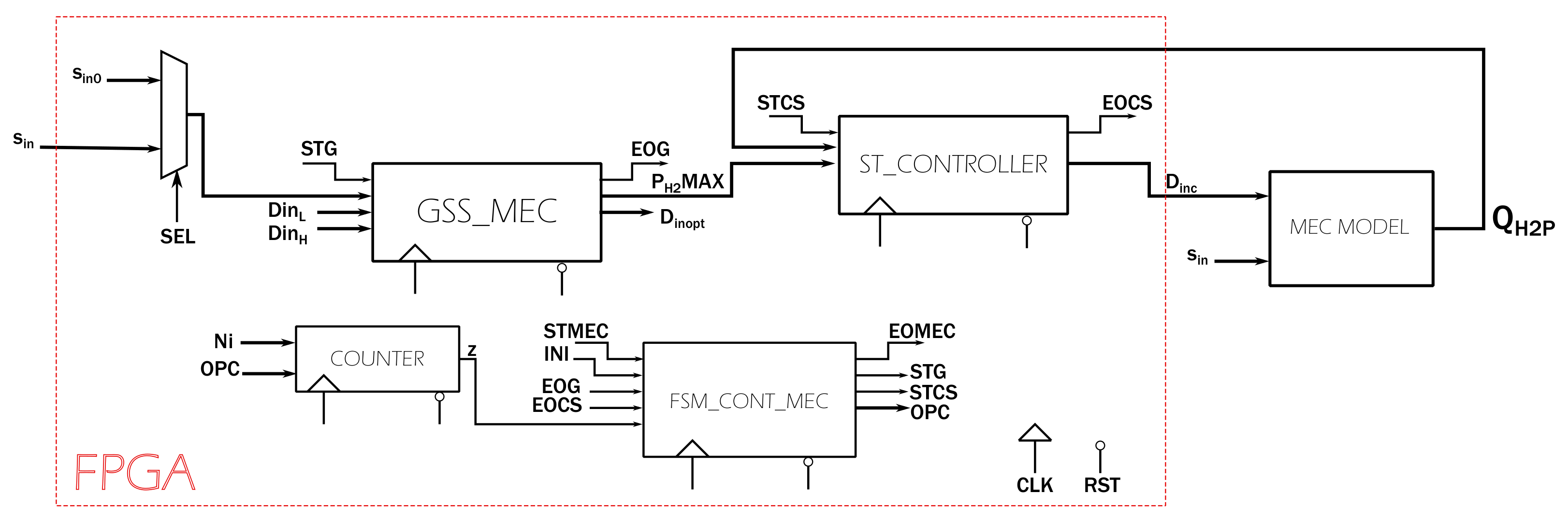
The FPGA-based implementation of the optimization algorithm is depicted in Figure 8 and Figure 9. Following the scheme presented in Figure 3, the implementation block diagram is integrated by the GSS algorithm digital architecture coupled to the DTSTC digital architecture. A finite state machine (FSM) and a down programmable counter are used to ensure the proper operation of the optimization algorithm embedded in the FPGA.

The digital architecture of the optimization algorithm uses a fixed point format (16,24) to represent all the input-output signals and inner operations. The hardware description used to develop the digital architecture was VHDL and the target board used was the Cyclone II EP2C35F672C6 integrated in the ALTERA DE2 educational board with a clock frequency $f_{CLK}=50$ MHz.

The modules GSS_MEC and ST_CONTROLLER were designed for an easy interaction with the FSM_CONT_MEC module and any other external device through the STG, EOG, STCS and EOCS signals. When the input signals STG and STCS are assigned to the logical value ‘1’ by the FSM_VCONT_MEC module, they will produce a busy mode of their respective modules due to the latency time in the calculation of their final results. The busy mode is indicated by the output signals EOG =’0’ and EOCS = ‘0’. On the other hand, when EOG = ‘1’ and EOCS = ‘1’, it means that the modules GSS_MEC and ST_CONTROLLER have finished and the results are ready to be read.

5.1. Operation of the FPGA-Embedded Optimization Algorithm

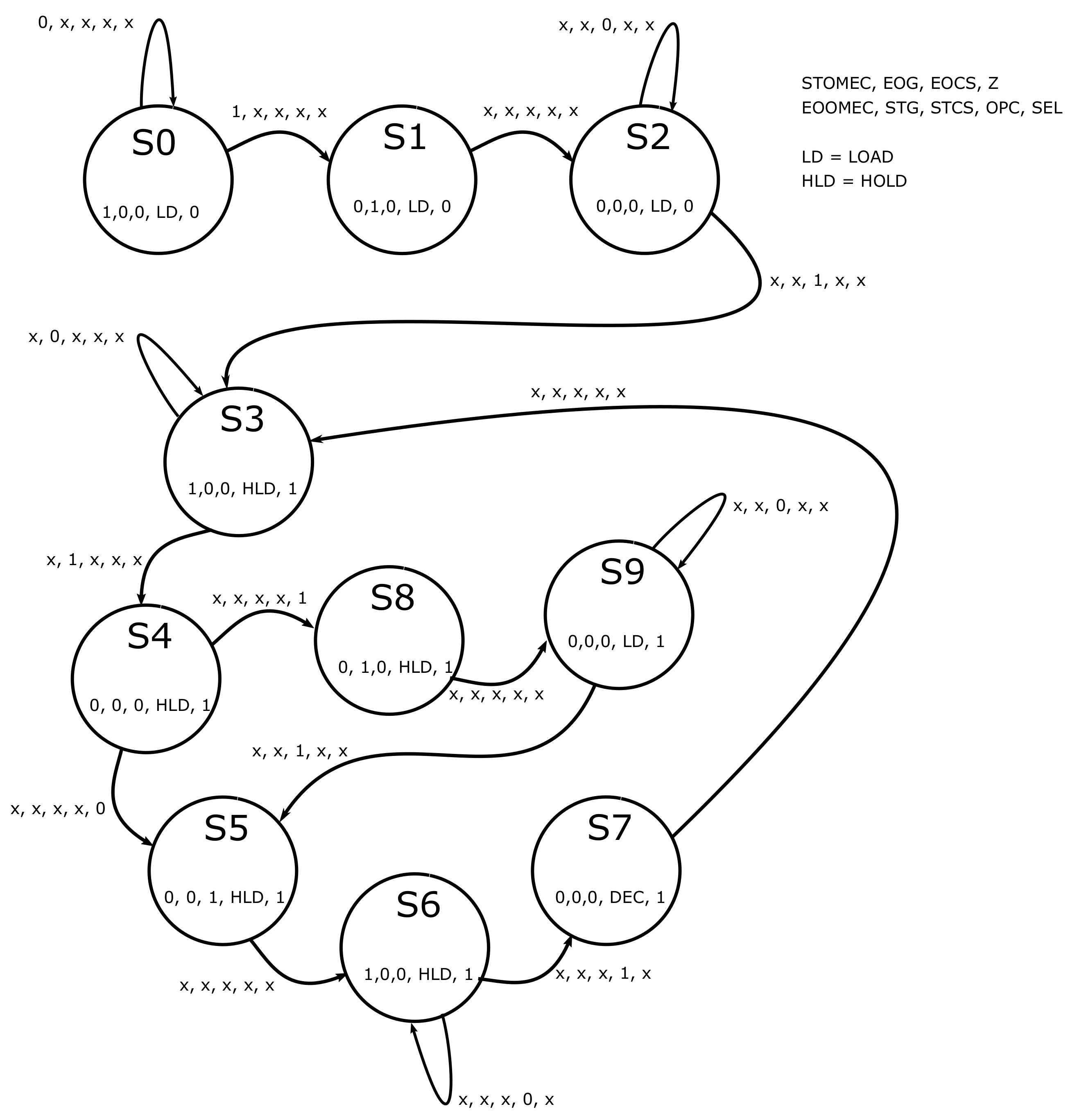
The FSM depicted in the Figure 9 is a great help for understanding the operation of the digital architecture. The FPGA execution can be divided in two steps, the initialization step, which is controlled by the states S0 to S2, and the normal operation, which is controlled by the remanding states of the FSM_CONT_MEC module. The initialization is executed when the FPGA is energized and the INI signal has a binary value ‘1’. Otherwise, the FPGA remains in standby mode until an external source changes the value of that signal. In such case, the initialization is started by a push-button (see the state S0). When INI = ‘1’ the FSM changes to the state S1 where STG = ‘1’ and SEL = ‘0’ in the GSS_MEC module and the two-one multiplexer. This will start the calculation of $Q_{H2,p,max}$ with the initial value $s_{in,0}$. In the next clock cycle, the EOMEC signal in the GSS_MEC module will change from logic ‘1’ to logic ‘0’ indicating that this module is in the process of calculating $Q_{H2,p,max}$. At the same time, without any condition, a transition is made to the state S2 where the FSM is waiting by the logic value ‘1’ in the EOMEC signal indicating that the result is ready. When $Q_{H2,p,max}$ is ready to be used by the ST_CONTROLLER module, the FSM make a transition to the state S3 where the initialization step is done, and the system now is in the normal operation where SEL = ‘1’ and it is waiting for an external device to set the value STOMEC = ‘1’. During the initialization step, the down counter is loaded with an initial value decreased by one every sampling period until reaching the optimization period.

In the normal operation, the ST_CONTROLLER module and the down counter are executed every sampling period with the aim of controlling the HPR in the MEC, and decreasing the initial value of the counter. When the down counter reaches the value zero, this means that the optimization period has expired and the GSS_MEC module is executed to generate a new $Q_{H2,p,max}$, after that, the down counter is reloaded with the initial value.

The normal operation starts in the state S3 and the digital architecture reads $s_{in}$ by SEL = ‘1’ in the multiplexer. When the signal STOMEC = ‘1’, the FPGA-based optimization algorithm generates the control input $D_{in,c}$ of the MEC after a latency time, otherwise, the system is in standby. The execution of the ST_CONTROLLER and the down counter are managed by the states S5 to S7 in the FSM every sampling period, while the states S8 and S9 manage the GSS_MEC MODULE and the reinitialization of the down counter when the optimization period has been reached. In order to know when the GSS_MEC module should be executed, the FSM reads the signal Z from the down counter in the state S4. When Z = ‘0’ this means that the optimization period has not yet elapsed and the FSM is currently executing the ST_CONTROLLER module, otherwise, when Z = ‘1’ the FSM executes one more time the GSS_MODULE and generates a new $Q_{H2,p,max}$ in function of the current value $s_{in}$. The down counter is reinitialized as well.

The most used arithmetic operations in the optimization algorithm are product, addition, division and square root. The hardware description was developed using standard VHDL and therefore the designs presented in this work do not belong to any manufacturer.

5.2. GSS Implementation

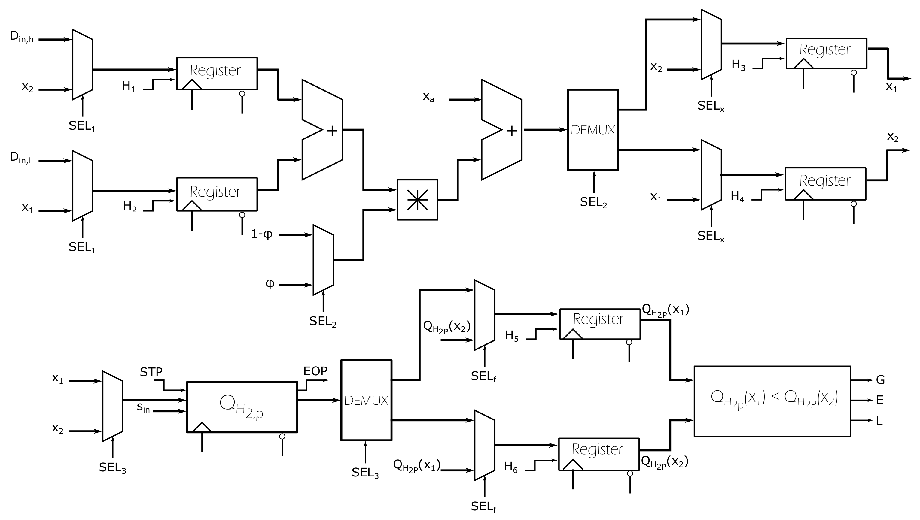
The digital architecture of the GSS optimization strategy, described in Algorithm 1, is depicted in Figure 10. The digital architecture of such algorithm is made up of registers, full adders, 8-bit embedded multipliers, multiplexers and full comparators using the previously mentioned fixed point format. Notice that the objective function shown in Equation (15) was programmed in the block $Q_{H2,p}$. Its implementation needed a simplified representation with the objective to calculate the hydrogen productivity with few hardware resources and small latency time. By precalculating constant parameters and making a separation by variables the following objective function is obtained:

$$Q_{H2,p}={\beta }_1{x}_a^{*}(s_{in},D_{in})\left({\beta }_2{\mu }_a\left(s^{*}\left(D_{in}\right)\right)+{\beta }_3\right),$$

(37)

where the values of constants ${\beta }_1$, ${\beta }_2$ and ${\beta }_3$ are defined in

Table 1. Constant parameters in $Q_{H2,p}$.

Constant Parameter	Value
β1	2.1906 × 10−8
β2	316.825
β3	40

.

The complete comparator that determines if $f_1>f_2$, in Algorithm 1, was designed taking into account that the operation involves real numbers and therefore the classical definition of a complete comparator of binary numbers is not sufficient for this implementation.

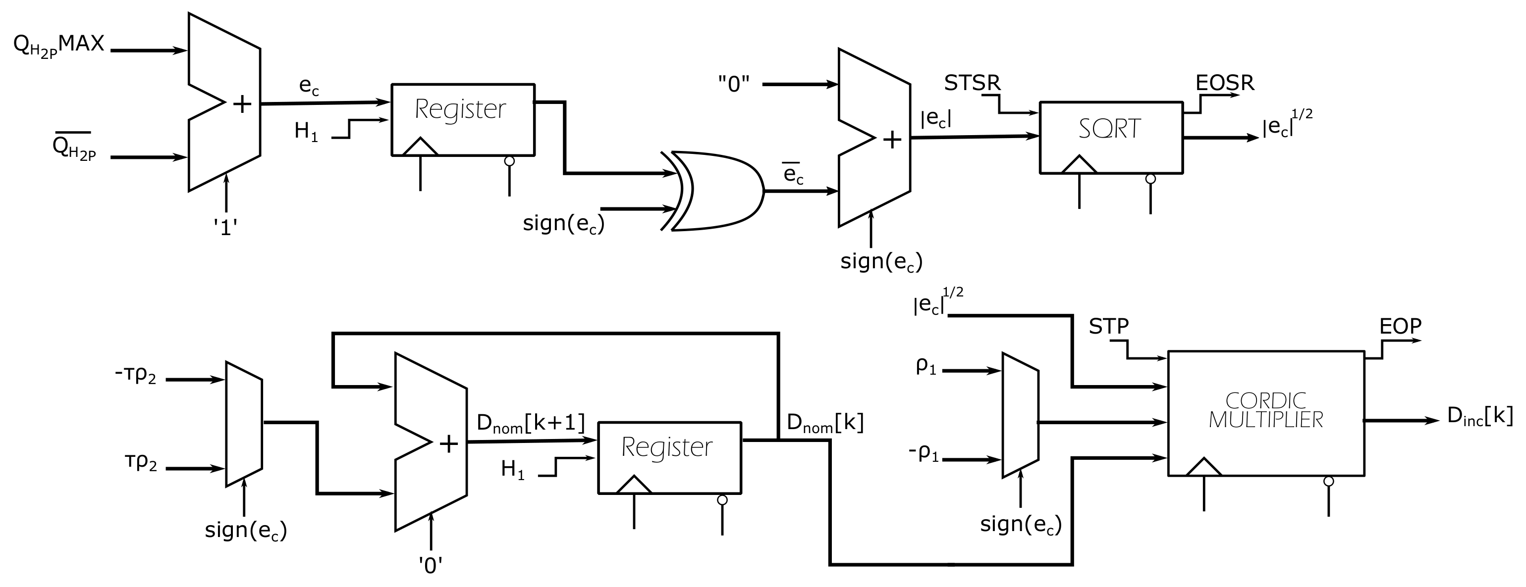
5.3. DTSTC Implementation

The digital architecture of the DTSTC (see Figure 11) is simpler than that one of the GSS algorithm. Although only combinational elements are required, its response speed is quite fast to generate the control action compared to the speed of change to generate the reference computed by the GSS algorithm.

The controller correction term ${\sigma }_1\sqrt{\left|ϵ\right|}$ requires a digital circuit capable of computing the square root of the tracking error. Particularly in this work, the Pencil and Paper algorithm [30] proved to be very useful as a basis for the design of the SQRT arithmetic circuit.

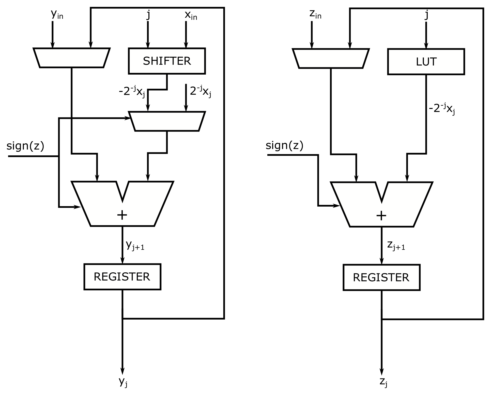
The arithmetic circuit of the multiplier in the DTSTC architecture is based on the Coordinate Digital Computer Algorithm (CORDIC) with its rotating linear version (see Figure 12) [31], i.e.,:

$$\begin{array}{ccc}\hfill x_{j+1}& =& x_j,\hfill \\ \hfill y_{j+1}& =& y_j+{\sigma }_j{2}^{-j}{x}_j,\hfill \\ \hfill z_{j+1}& =& z_j+{\sigma }_j{2}^{-j},\hfill \end{array}$$

(38)

with

$${\sigma }_j=\left\{\begin{array}{cc}-1\hfill & if z_j\ge 0\hfill \\ +1\hfill & otherwise.\hfill \end{array}\right.$$

(39)

The results obtained after a sequence of fixed micro-rotations are given in the following way:

$$\begin{array}{ccc}\hfill x_f& =& x_{in},\hfill \\ \hfill y_f& =& y_{in}+x_{in}{z}_{in}\hfill \\ \hfill z_f& =& 0.\hfill \end{array}$$

(40)

The resulting operation $y_f$ in Equation (40) has the necessary shape to implement the DTSTC. As it can be seen in Equation (35), $D_{in,c}$ can be calculated from the final result $y_f$ by these two arithmetic operations; i.e., the product and the addition. The CORDIC-based Multiplier Digital Circuit presented in the Figure 12 has the shape necessary to implement DTSTC without the need of using embedded multipliers in the FPGA and it has a short latency time.

6. Results

The feasibility of the FPGA-embedded optimization algorithm was demonstrated through numerical simulations. The MEC model (1)–(6) was simulated in Matlab, the ODEs were solved by the stiff solver ode15s. The parameters used in the numerical simulations are listed

Table 2. MEC Model parameter with uncertainties.

Description	Symbol	Value	Variation (%)
Gas ideal constant (J mol−1K−1)	R	8.31	0.00
Faraday constant (C mol−1e−1)	F	96,485	0.00
Temperature (K)	T	298.15	−20.00
Yield coefficient (mg (s) mg−1 $\left(x_a\right)$)	$k_a$	0.667	+15.00
Yield coefficient (mg (s) mg−1 $\left(x_m\right)$)	$k_m$	4.7067	−20.00
Microbial decay (d−1)	$k_{d,a}$	0.05 ${\mu }_{max,a}$	+5.00
Microbial decay (d−1)	$k_{d,m}$	0.05 ${\mu }_{max,m}$	+2.00
Biofilm retention constant of $x_a$	${\alpha }_a$	0.5	+12.00
Biofilm retention constant of $x_m$	${\alpha }_m$	0.5	+5.00
Maximum grown rate (d−1)	${\mu }_{max,a}$	1.97	+28.00
Maximum grown rate (d−1)	${\mu }_{max,a}$	0.30	+ 14.00
Half-rate constant (mg (s) L−1)	$k_{s,a}$	20	+15.00
Half-rate constant (mg (s) L−1)	$k_{s,m}$	80	−15.00
Local potential (V)	$\eta$	0.3	+10.00

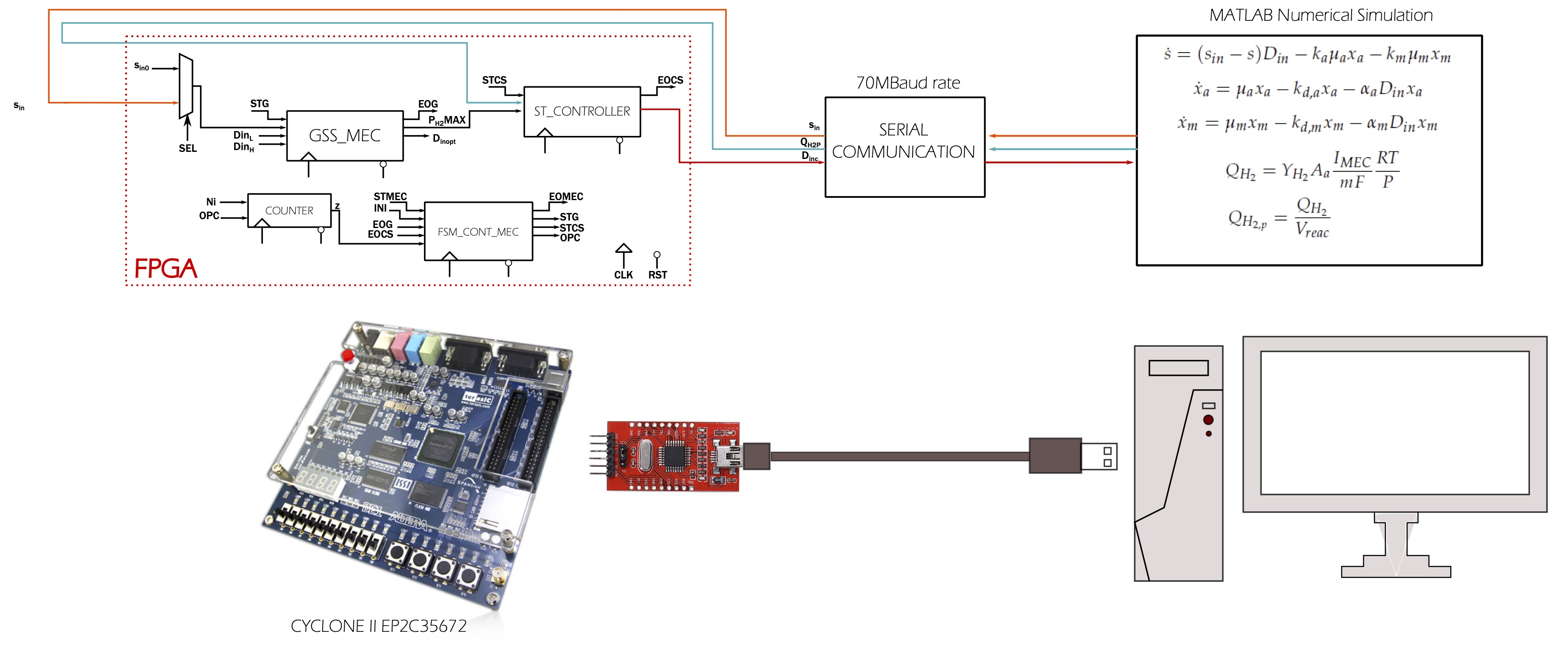
. In order to demonstrate the robustness of the optimization strategy proposed, modified parameters between $\pm 30\%$ from their nominal value were considered. The hardware required for the verification test is depicted in the Figure 13. As it can be seen, a serial communication was used to communicate the FPGA with Matlab, which was executed in a personal computer with Windows 10, Intel Core i7 and memory RAM DDR3 of 32 GB. In these conditions, six hours were needed to perform the verification test of the optimization algorithm in a Cyclone II FPGA running at $f_{clock}=50 \mathrm{MHz}$ and a reception-transmission data rate of $70 \mathrm{Mbps}$. The operation time of the MEC simulated in the computer was of 200 d with a sampling period $\tau =0.004 d$. The hardware resources in the target board are summarized in

Table 3. Specifications of the FPGA ALTERA DE2.

Device	Digital Elements	Total Resources
	Logic Elements (L.E.)	33,216
	Registers	3967
EP2C35F672C6	Number of pins	475
	Embedded Multipliers	70
	RAM bits (Kb)	4
	PLLs	4
	$f_{max,CLK}$	120 MHz
FPGA	RS-232 transceiver and 9-pin connector	120 Kbits/s
	Expansion Headers	two 40-pin
	Toggle switches	18
	Push button switches	4

.

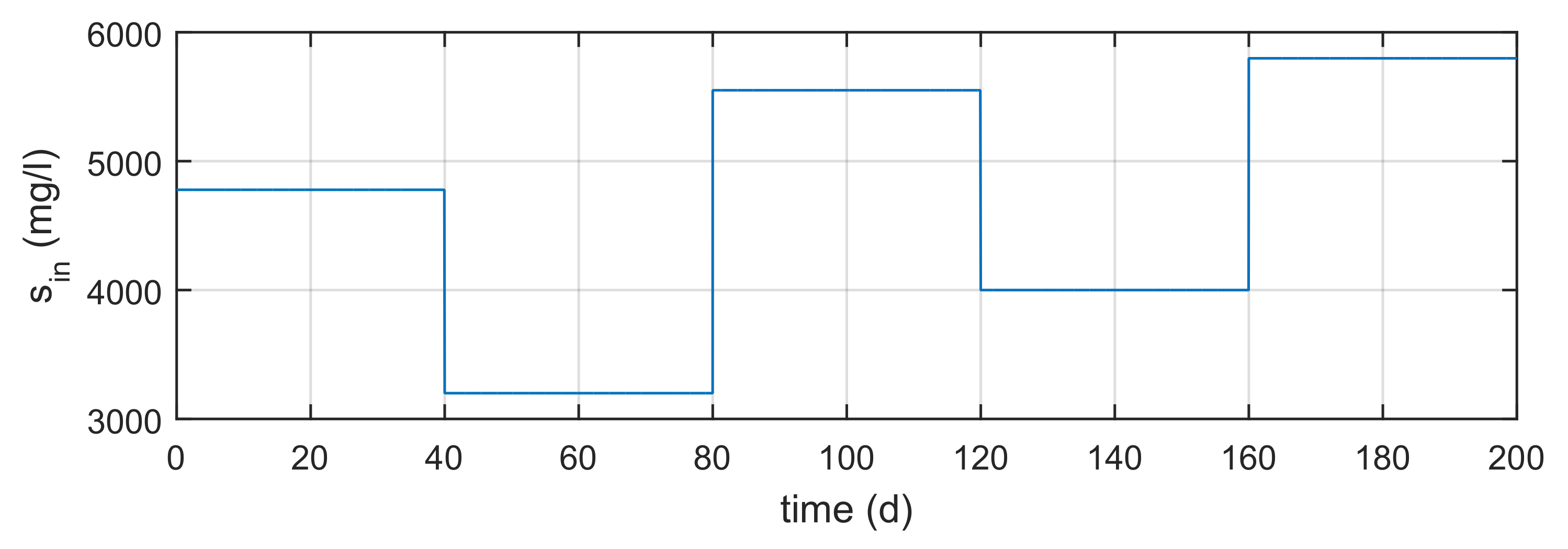
The inlet acetate concentration $s_{in}$ used to feed the MEC in the numerical simulations is depicted in Figure 14. The digital architecture verification test of the MEC optimization algorithm consists mainly in comparing the results obtained from the FPGA working with the fixed point format (16,24) with the results of the same algorithm executed in Matlab in a floating point representation format.

The resulting HPR obtained by executing the optimization algorithm both in the FPGA and in Matlab is shown in Figure 15. The green dashed-line represents the HPR by the MEC model, the red line represents the maximum HPR computed in Matlab, while the blue dashed-line represents the maximum HPR computed by the FPGA.

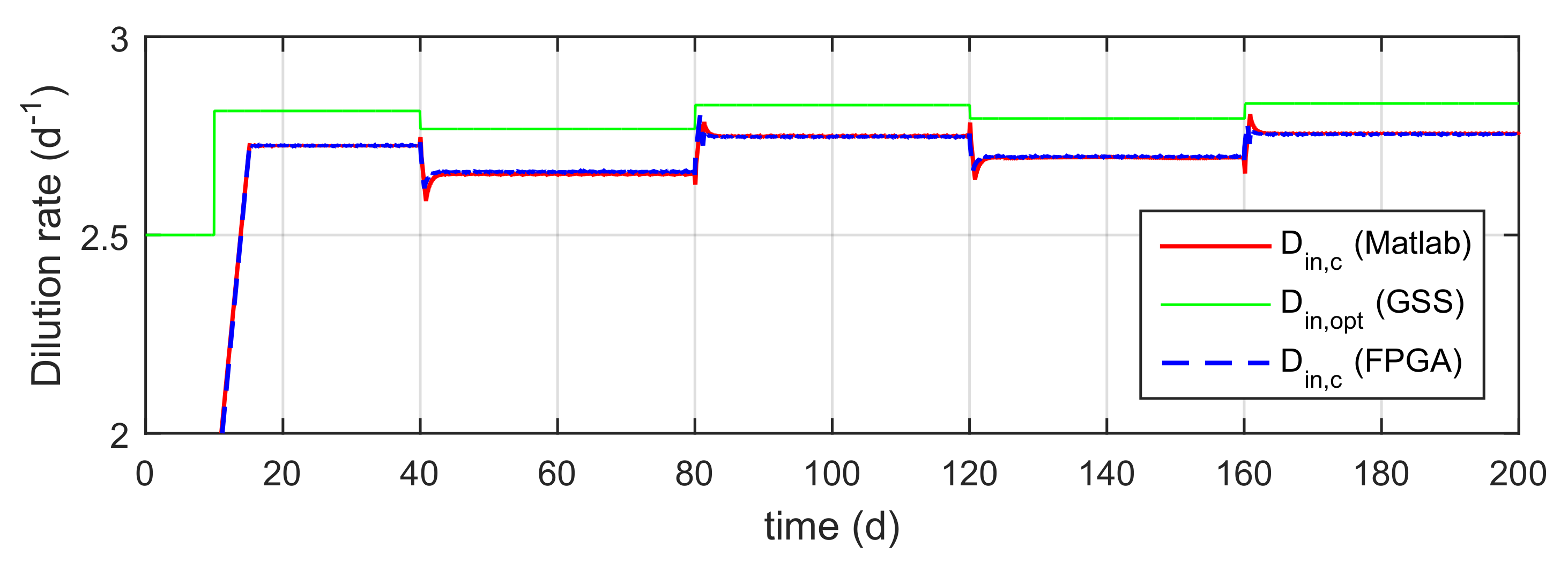
On the other hand, the dilution rate computed by the optimization algorithm both in the FPGA and in Matlab is shown in Figure 16. The green dashed-line represents the optimum dilution rate computed by the GSS algorithm, the red line represents the dilution rate computed by the DTSTC in Matlab, while the blue dashed-line represents the dilution rate computed by the DTSTC in the FPGA. As it can be seen, the numerical representation format used to design the optimizer’s digital architecture reduces properly the truncation error due to the finite number of bits.

Initially, the optimization algorithm requires eighteen days to reach the optimal point, as shown in Figure 15. The super-twisting controller requires this period for the control error to converge to zero using the gains specified in

Table 4. Discrete time super-twisting controller gains.

Gain	Value
${\rho }_1$	0.09
${\rho }_2$	0.19

. In this transitory period, the GSS algorithm is initialized with 105 mL [$H_2$] mL⁻¹d⁻¹ and this value was taken as the initial reference for the DTSTC.

Once the tracking error has converged to zero, the GSS algorithm reads the inlet acetate concentration value $s_{in}$, every optimization period equivalent to $D_{in,max}^{-1}=0.33$ d to update the maximum productivity value $Q_{H2,pmax}$ used as reference by the DTSTC.

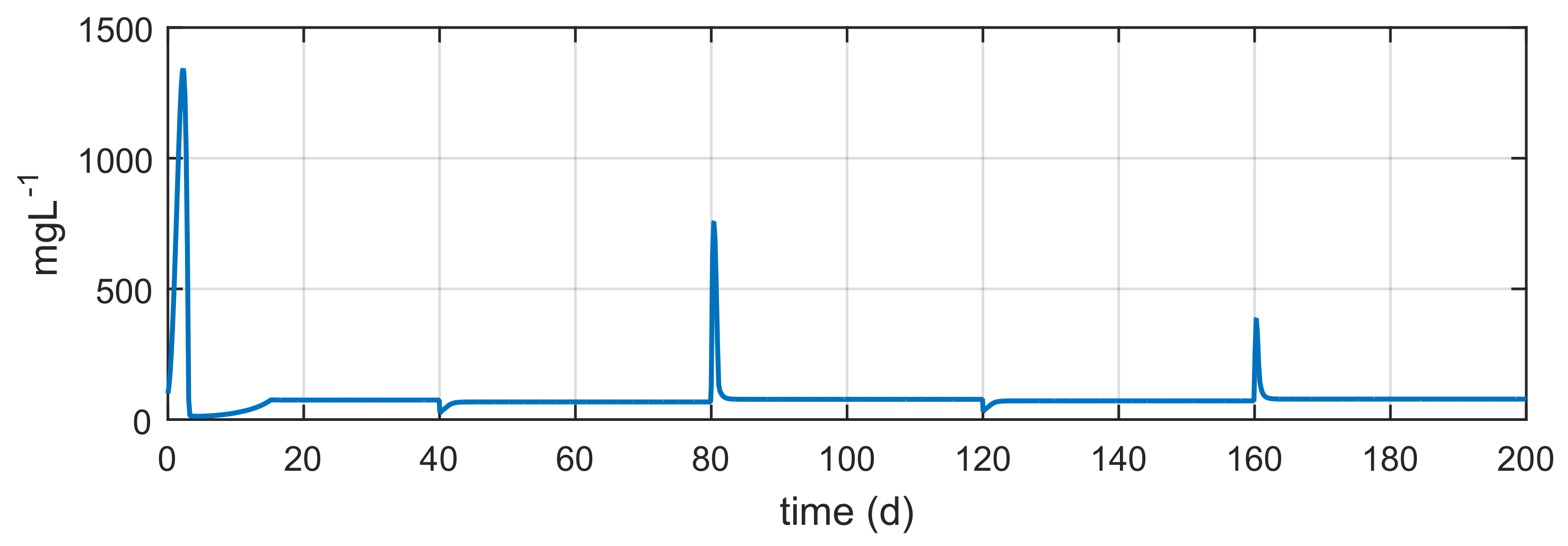
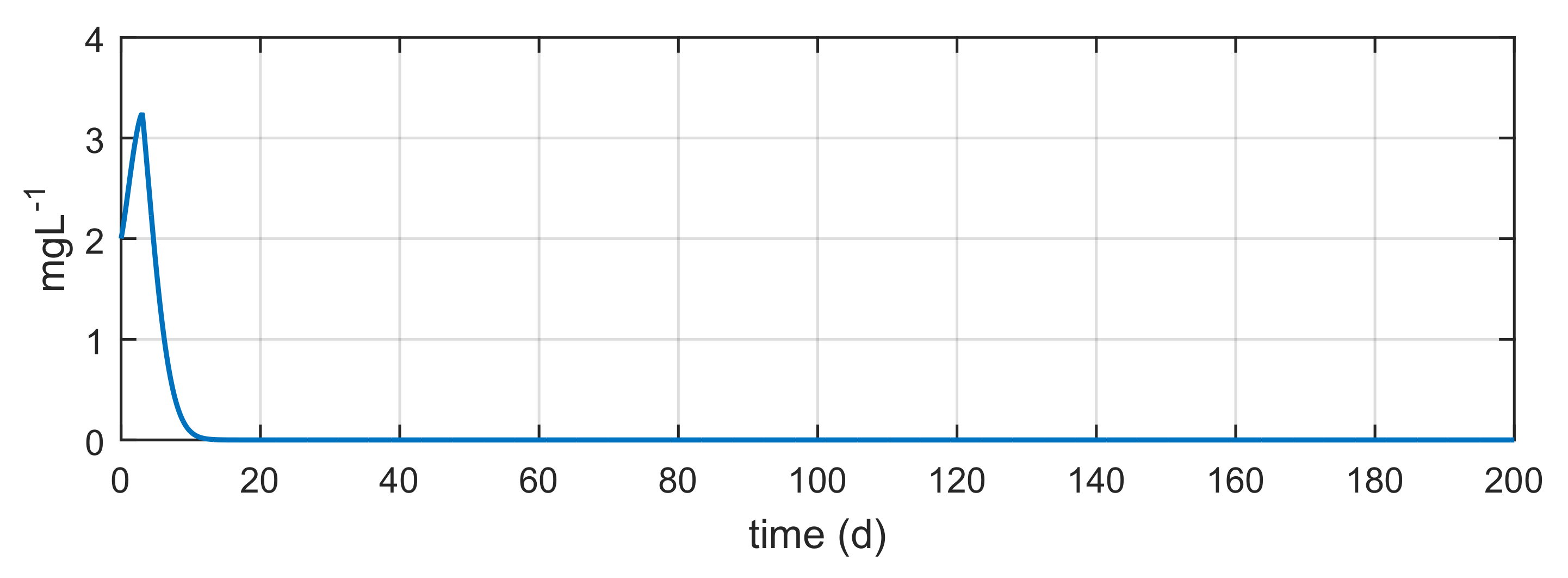
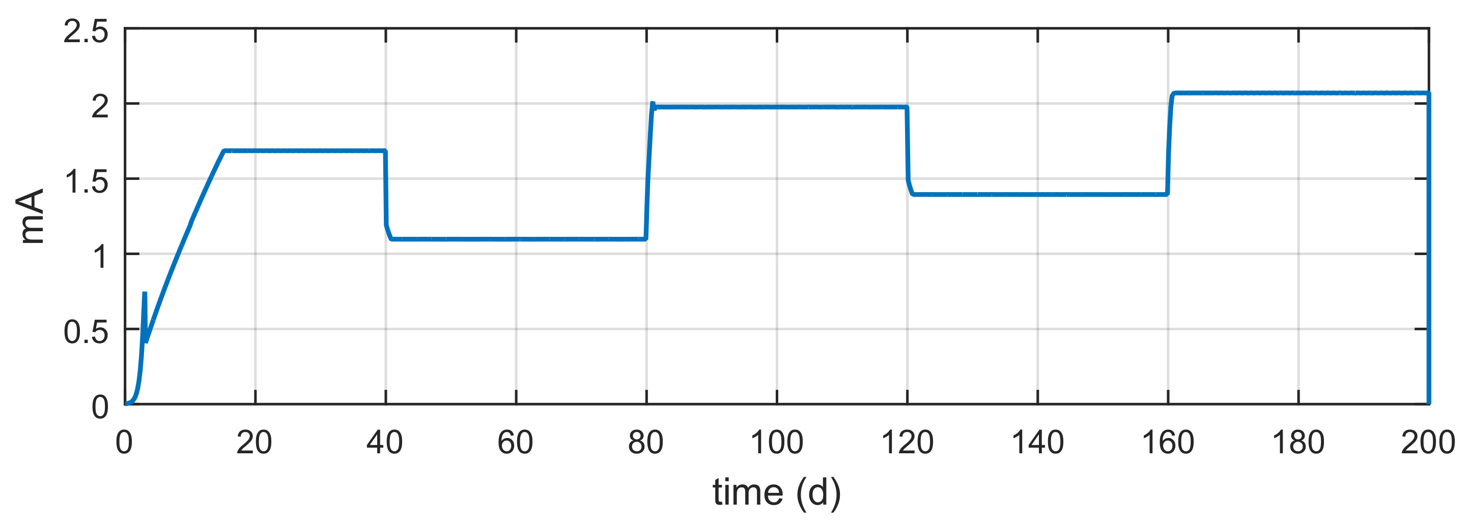
The acetate concentration in the MEC is showed in the Figure 17. It is easy to see in Figure 18 and Figure 19 that the most of the acetate used to feed the MEC is consumed by the anodophilic bacteria $x_a$ because there is a inhibition process in the methanogenic bacteria growing $x_m$. As expected, the current between the MEC electrodes is closely related to the HPR (see Figure 20).

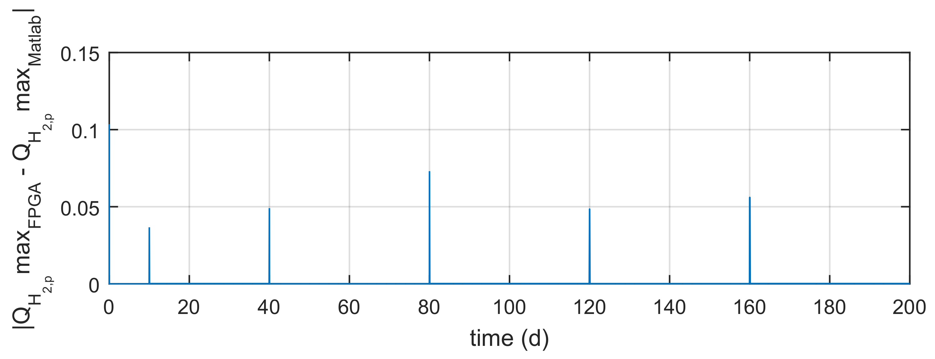
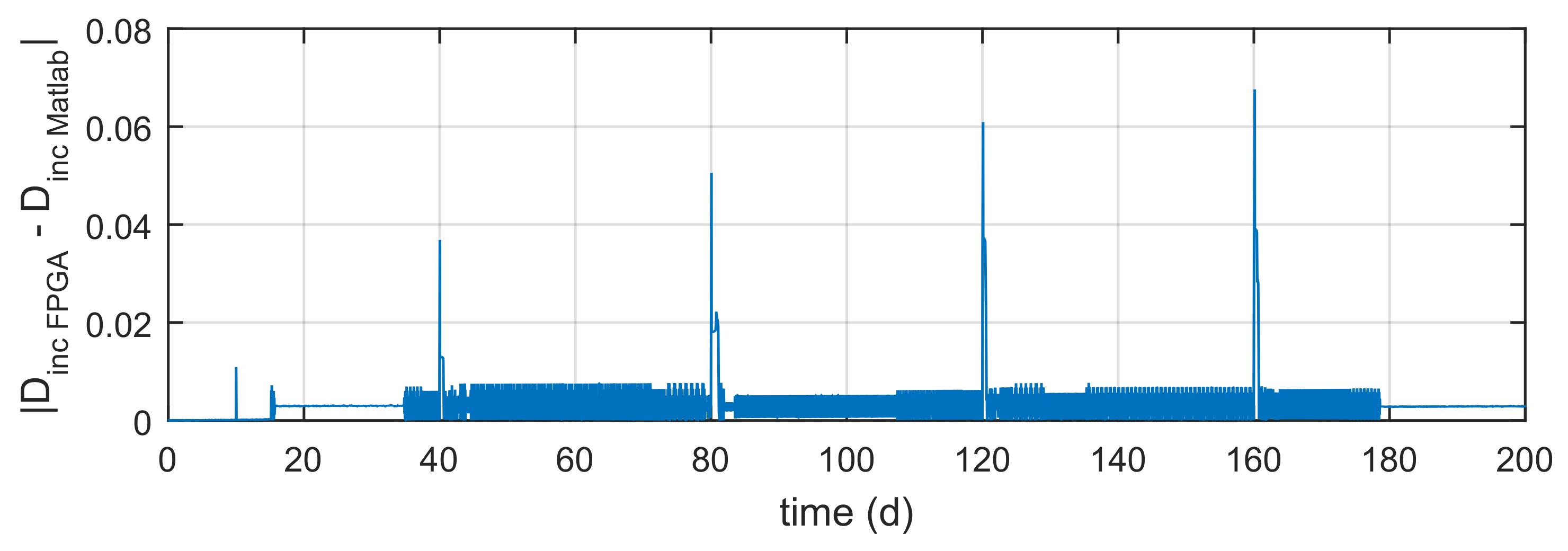
6.1. Error Analysis

The truncation error in the digital architecture of the optimization algorithm is mainly due to the bits fixed quantity in the representation format established in this work. If the resolution in the intermediate operations required to run the optimization algorithm on the FPGA is not sufficient, the truncation error will propagate in such a way that the results obtained are greatly affected.

Figure 21 and Figure 22 show the behavior of the truncation error throughout the simulation process. It can be seen that the error is small enough to determine that the (16,24) format is sufficient to implement the optimization algorithm architecture in the FPGA.

6.2. Hardware Report

The FPGA hardware resources needed for embedding the digital architecture of the optimization algorithm on Figure 8 are summarized in

Table 5. Hardware resources used by the optimization algorithm.

Digital Elements	Resources	Used	%
Total L.E.		7089	21.34%
Register only	33,216	291	0.87%
LUT/Register		1472	4.43%
D.L.R.		1724	5.19%
M4K	483,340	0	0.00%
8b-Mult.	70	45	64.00%
I-O delay (No. cycles)	50 MHz	7500	150 μs

. Only a 21% of the total logic elements (L.E.), 5.19% of dedicated logic registers (D.L.R.) and 64% of total eight-bits multipliers (8b-Mult.) in the chip Cyclone II were used. The input to output delay in the implementation was of $150$ μs. The estimated power consumption required by the EP2C35F672C6 device using the aforementioned hardware resources is 146 mW. This estimate was calculated by the PowerPlay Early Power Estimator spreadsheet for Cyclone II family v8.0 SP1.

The hardware resources used by the most important functional blocks in the optimization algorithm are summarized in

Table 6. Hardware resources used by GSS algorithm.

Digital Elements	Resources	Used	%
Total L.E.		5849	17.60%
Register only	33,216	191	0.57%
LUT/Register		1044	3.14%
D.L.R.		1235	3.71%
8b-Mult.	70	45	64.00%
I-O delay (No. cycles)	50 MHz	7500	150 μs

,

Table 7. Hardware resources used by $Q_{H2,p}$ block.

Digital Elements	Resources	Used	%
Total L.E.		5180	15.59%
Register only	33,216	183	0.55%
LUT/Register		727	2.18%
D.L.R.		910	2.74%
8b-Mult.	70	34	48.57%
I-O delay (No. cycles)	50 MHz	249	4.97 μs

and

Table 8. Hardware resources used by DTSTC algorithm.

Digital Elements	Resources	Used	%
Total L.E.		1165	3.51%
Register only	33,216	100	0.30%
LUT/Register		374	1.13%
D.L.R.		473	1.42%
8b-Mult.	70	0	0.00%
I-O delay (No. cycles)	50 MHz	200	4 μs

. As it can be seen in Table 6 and Table 7, 64% of the total 8-b multipliers in the FPGA are used in the GSS algorithm, where 48.57% is destined to the $Q_{H2,p}$ functional block where the objective function defined by Equation (15) is processed. It should be pointed out that the $Q_{H2,p}$ block is part of the GSS algorithm functional block (see Figure 10). The GSS algorithm needs at least 4 cycles in the worse of the cases to reach the tolerance error (err = 0.001) defined by Equation (20). Therefore, embedded multipliers most be used in the GSS algorithm digital architecture to have a short latency time.

On the other hand, the hardware resources used in the DTSTC and its inner functional block, the CORDIC Multiplier, are summarized in Table 8 and

Table 9. Hardware resources used by CORDIC multiplier.

Digital Elements	Resources	Used	%
Total L.E.		900	2.70%
Register only	33,216	99	0.30%
LUT/Register		219	0.66%
D.L.R.		300	0.90%
8b-Mult.	70	0	0.00%
I-O delay (No. cycles)	50 MHz	74	1.48 μs

. Most DTSTC inner operations are implemented using a CORDIC-based multiplier that has a latency time of 1.48 μs in the worse of the cases, before the tracking error converges to zero. After that, the multiplier is executed faster than 1.48 μs. It should be noted that the CORDIC-based multiplier internally uses an 8-bit expansion in the fractional part to substantially improve the truncation error generated by the fixed-point format considered (see Figure 22).

Finally, the arithmetic operation $\sqrt{\left|ϵ\right|}$ in the DTSTC is processed by the SQRT functional block, which is based on the Pencil and Paper algorithm. Its digital architecture is primarily based on bit additions and shifts.

Table 10. Hardware resources used by SQRT.

Digital Elements	Resources	Used	%
Total L.E.		153	0.46%
Register only	33,216	1	0.00%
LUT/Register		89	0.26%
D.L.R.		90	0.27%
8b-Mult.	70	0	0.00%
I-O delay (No. cycles)	50 MHz	74	1.3 μs

shows the hardware resources needed.

7. Conclusions

In this work an FPGA-embedded optimization algorithm to maximize the hydrogen production rate (HPR) of a microbial electrolysis cell (MEC) using the golden section search (GSS) algorithm coupled to a discrete-time super-twisting controller (DTSTC) was presented. The correct performance of the GSS algorithm was analyzed analytically. Furthermore, it was proven that the relative degree of the MEC model is one, a necessary condition to use the DTSTC to bring the HPR to its maximum performance point in finite time.

To reduce the power consumption required to bring the MEC to its maximum performance, a digital architecture of the optimization algorithm was designed and embedded in an FPGA. Although the FPGA used in this work was the Cyclone II of ALTERA, the digital architectures presented in this work were designed to be implemented in any FPGA, regardless of the manufacturer.

The results of the FPGA-embedded optimization algorithm showed a correct performance with low hardware resources and low power consumption compared with a personal computer. Besides, the truncation error generated by the fixed point format used in this work was practically negligible.

Such results allow us to conclude that the implementation of control and optimization algorithms in FPGAs represents an excellent alternative to replace personal computers. Particularly, as demonstrated in the previous section, the FPGA-embedded optimization algorithm proposed to maximize the HPR in the MEC, represents a lower cost alternative in terms of consumed power and resources.