A Time-Series Data Generation Method to Predict Remaining Useful Life

Abstract

Accurate predictions of remaining useful life (RUL) of equipment using machine learning (ML) or deep learning (DL) models that collect data until the equipment fails are crucial for maintenance scheduling. Because the data are unavailable until the equipment fails, collecting sufficient data to train a model without overfitting can be challenging. Here, we propose a method of generating time-series data for RUL models to resolve the problems posed by insufficient data. The proposed method converts every training time series into a sequence of alphabetical strings by symbolic aggregate approximation and identifies occurrence patterns in the converted sequences. The method then generates a new sequence and inversely transforms it to a new time series. Experiments with various RUL prediction datasets and ML/DL models verified that the proposed data-generation model can help avoid overfitting in RUL prediction model.

1. Introduction

Prognostics and health management (PHM) is an important contributor to maintaining manufacturing productivity and has rapidly evolved from corrective maintenance to condition-based maintenance (CBM). Also known as predictive or data-driven maintenance, CBM decisions are based on analysis of data gathered from equipment and sensors [1].

The established applications of CBM are monitoring, fault diagnosis, maintenance scheduling, and remaining useful life (RUL) prediction [2]. Among them, RUL prediction is the subject of growing interest because of its effectiveness in maintenance scheduling. The RUL can be defined as the difference between the current time and the time failure occurs, and RUL prediction is to predict RUL (or failure time) at the current time based on collected signals, condition, and so forth [3]. The RUL prediction techniques can be categorized into physical model-driven and data-driven techniques [4].

Zhu and Yang [5] computed the themo-elasto-plastic stress and strain fields of turbine blade using finite element methods. They predicted the fatigue life through Basquin and Manson–Coffin formulae. They performed the thermal stress field analysis by using of Ansys software and then diagnosed thermal–mechanical stress for some nodes. Then, they predicted the fatigue life by maximum stress and mean stress. The remaining lifetime was predicted by extracting the parameter of the formula from controlled stress test data. While they introduced the influence of limited external factors such as thermal and mechanical stress on the remaining life, we consider the state as a time series and predicted the remaining life in a continuous situation probabilistically. Taheri and Taheri [6] studied the feasibility and technical design for implementing a combined heat and power system for the Mahshad Power plant. They figured out the remaining life for gas turbines on the basis of available data by approximated approach, whose prediction is derived by using predetermined elements or formulae. In addition, they used the operation data reflecting the current status for prediction, while our method in this paper adopts a probabilistic approach and uses obtainable data rather than deriving the close-formed formula.

Even though the physical model is easy to understand and very accurate, it is almost impossible to formulate modern industrial system. In contrast, the data-driven technique using machine learning (ML) and deep learning (DL) can formulate a very complex system with data collected from the system. For this reason, this paper focuses on data-driven RUL prediction.

Recently, ML and DL models have been frequently applied to predict RUL after training them with run-to-failure data [7]. These models learn the degradation patterns and relationships between the pattern and the RUL from the data collected until the end of the life of the components and predict the RUL of target components. In many recent studies, ML and DL models have shown superior performance for RUL problems [8,9,10,11,12,13,14,15].

Data insufficiency is a major challenge when training ML- or DL-based RUL models. Because a time-series sample is collected only after a component fails, collecting training data tends to be time-consuming and expensive. A model trained with insufficient data can be overfitted [16] and fail to accurately predict the RUL of a new component. Collecting more data can mitigate overfitting but may not be an option because of the required time and cost.

In this paper, we propose a time-series data-generation method that avoids overfitting when training an RUL model. The proposed method generates a sample on the basis of two existing samples called parents in a probabilistic manner and contributes to avoiding overfitting and increasing prediction performance. The generated samples will be added to training data for an RUL prediction model and contribute to avoid overfitting. In other words, an RUL prediction model is trained with union of original samples and generated samples. This approach is similar to SMOTE (Synthetic Minority Over-sampling Technique [17]), one of the most widely used oversampling methods that generates a minority class samples between two selected samples at random, and accordingly, the generated one may not be similar to the original samples in terms of relationship among features while contributing to the increase of classification performance such as recall and F1-score.

As far as our literature survey is concerned, ours is the first attempt to address the data insufficiency problem when training an RUL prediction model. In this paper, we propose a method to transform a time series into an alphabetical sequence and inversely transform the sequence that can be applied in time-series classification and clustering. The proposed data-generation method is not only efficient (i.e., it is inexpensive in terms of computational time) but also effective (i.e., the generated time series cab help avoid overfitting).

The remainder of this paper is organized as follows. Section 2 introduces background theory and related works of RUL prediction and symbolic aggregate approximation. Section 3 proposes a time-series data-generation method for RUL prediction in detail, and Section 4 illustrates the process of the proposed method using a small example. Section 5 experimentally verifies the performance of the proposed method, and Section 6 draws conclusions and suggests future research directions.

2. Background Theory and Related Works

2.1. Remaining Useful Life Prediction

Training and usage process of the RUL prediction model proceeds as follows. First, a set $\mathrm{X}=\left\{{\mathit{x}}^{\left(1\right)}, {\mathit{x}}^{\left(2\right)}, \cdots ,{\mathit{x}}^{\left(n\right)}\right\}$ of training time series samples ${\mathit{x}}^{\left(i\right)}, i=1,2, \cdots ,n$ is transformed by extracting features and the RUL such that:

$$D\left(X\right)={{\displaystyle \bigcup }}_{i=1}^{n}D\left({\mathit{x}}^{\left(i\right)}\right),$$

(1)

where $D\left(X\right)$ is a set of transformed time series in $X$, and $D\left({\mathit{x}}^{\left(i\right)}\right)$ is a set of pairs (feature, RUL) extracted from ${\mathit{x}}^{\left(i\right)}$:

$$D\left({\mathit{x}}^{\left(i\right)}\right)=\left(\mathbf{\varphi }\left({\mathit{x}}_{1:t}^{\left(i\right)}\right), y_t^{\left(i\right)}\right),$$

(2)

where $\mathbf{\varphi }$ is a vector of feature functions, ${\mathit{x}}_{1:t}^{\left(i\right)}$ is a part of the time series collected from time 1 to $t$ of sample $i$, $y_t^{\left(i\right)}=\frac{T_i-t}{T_i}$ is the RUL of sample $i$ measured at $t$, and $T_i$ is the length of ${\mathit{x}}^{\left(i\right)}$. Second, a model $f$ is trained using $D\left(X\right)$, and finally, the RUL of the new sample $n+1$ at $t$ is predicted as $f\left(\mathbf{\varphi }\left({\mathit{x}}_{1:t}^{\left(n+1\right)}\right)\right)$.

Many researchers have developed RUL prediction models based on ML or DL. For example, Ali et al. [18] introduced a root mean square entropy estimator (RMSEE), which is the entropy of the root mean square (RMS) of the $j^{\mathrm{th}}$ windows, to capture bearing degradation and used it as a feature. They also converted an RUL prediction model into a classification problem with seven classes according to the degradation rate (that is, class 1: under 10%, class 2: 10%–25%, class 3: 25%–40%, class 4: 40%–55%, class 5: 55%–70%, class 6: 70%–85%, and class 7: 85%–100%). Finally, they used a multi-layered perceptron (MLP) combined with a simplified fuzzy adaptive resonance theory map as a prediction model. Zheng et al. [19] pointed out that a traditional regression model using features from a window is not appropriate for RUL prediction because it does not fully consider sequence information, and other sequence learning models have also flaws (e.g., hidden Markov model and recurrent neural networks do not consider long-term dependency among nodes). They proposed a deep long short-term memory (LSTM) consisting of four layers: an input layer, a multi-layer LSTM, a multi-layer perceptron (MLP), and an output layer. In their experiment, MLP, support vector regression (SVR), relevance vector regression, and a convolutional neural network were compared in terms of root mean squared error (RMSE), with the deep LSTM exhibiting the smallest RMSE for four datasets.

Table 1. Previous studies on RUL prediction.

Research	Domain	Feature	Base Model
[18]	Bearing	RMSEE	MLP
[19]	General	Original	LSTM
[20]	Bearing	Original	CNN
[21]	Rotating machine	RMS, kurtosis, etc.	MLP
[22]	Bearing	Spectral kurtosis	SVR
[23]	Data	RMS, peak, kurtosis, crest factor, etc.	SVR
[24]	Bearing	RMS and kurtosis	LSTM

General: not considering specific industry domain; original: not using specific feature functions but using raw values.

summarizes previous research that developed RUL prediction models using ML and DL including convolution neural network (CNN), in terms of domain, feature, and base model. As seen Table 1, statistics such as RMS, kurtosis, and skewness are frequently used as features, and MLP, LSTM, and SVR are used primarily for models.

2.2. Symbolic Aggregate Approximation

Pattern extraction is very important for time series analysis such as classification and clustering, but it is hard to extract patterns directly from time series due to huge search space [25]. Thus, representation methods such as symbolic aggregate approximation (SAX), discrete cosine transform (DCT), and discrete wavelet transform (DWT) are usually used to represent time series as sequence before pattern extraction. In this paper, each time series is discretized as alphabet sequence using SAX, patterns are extracted from the sequences, and a new sequence is generated considering the extracted pattern.

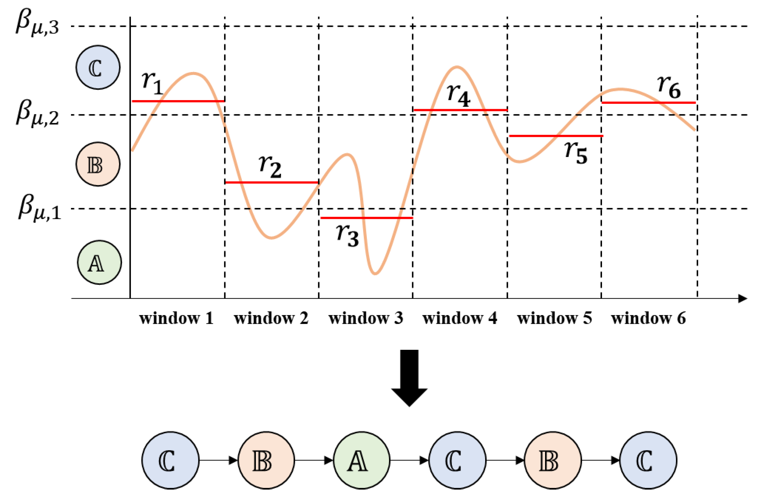
SAX can convert a time series $x$ into an alphabetical sequence $\mathrm{S}$ for efficient time-series data mining in the following manner [26]. First, the $t^{\mathrm{th}}$ element $x^t$ of $x$ is normalized as ${\tilde{x}}^t=\frac{x^t-\mu }{\sigma }$, where $\mu$ and $\sigma$ denote the mean and standard deviation of $x$, respectively. Second, ${\tilde{x}}^t$ is split into $w$ windows and$r=\left(r_1, r_2,\cdots ,r_w\right)$, where $r_j, 1\le j\le w$ is a representative value such as the mean of the values in the $j^{\mathrm{th}}$ window, is calculated. One can introduce the standard deviation as the alternative representative value. Third, break points ${\beta }_k$ for $k=1, 2, \cdots , l$ are computed, where $l$ is the number of alphabetical strings defined by the user, satisfying $\mathrm{Pr}\left({\beta }_k\le r_j<{\beta }_{k+1}\right)=1/l$. Finally, an alphabet is assigned to each window on the basis of the break points. That is, if ${\beta }_k\le r_j<{\beta }_{k+1}$, then the $k^{\mathrm{th}}$ alphabet string is assigned to the $j^{\mathrm{th}}$ window.

Figure 1 illustrates a SAX application process when the time series is assumed to be normalized. Time series is split into $w=6$ windows, and mean values $r_1, r_2, \cdots , r_6$ in each window are calculated. Three ($l=3$) alphabetical strings $\mathbb{A}$, $\mathbb{B}$, and $ℂ$ are introduced, and then three break points ${\beta }_{\mu ,1}$, ${\beta }_{\mu ,2}$, ${\beta }_{\mu ,3}$ for means are obtained. Then, the alphabet $\mathbb{A}$ is assigned to those means less than ${\beta }_{\mu ,1}$, $ℂ$ to those bigger than ${\beta }_{\mu ,2}$, and $\mathbb{B}$ to those between ${\beta }_{\mu ,1}$ and ${\beta }_{\mu ,2}$. Then, we obtain a sequence S = $ℂ$ − $\mathbb{B}$ − $\mathbb{A}$ − $ℂ$ − $\mathbb{B}$ − $ℂ$ of alphabetical strings that is converted from the time series.

SAX has been used to extract features from time series for various tasks such as classification and clustering. For example, Georgoulas et al. [27] extracted alphabetical features to represent the vibration of bearings and used them to detect bearing faults with various classifiers. Park and Jung [28] proposed a method to reveal rules from multivariate time series. It transforms a time series to an alphabetical sequence through SAX and identifies frequent patterns from the sequences using association rule mining. Notaristefano et al. [29] made groups of electrical load pattern by reducing data size using SAX.

3. Proposed Data Generation Method

This section explains the proposed three-phase data-generation method: preprocessing, generating an alphabetical sequence, and generating time-series values. In the first phase, every time-series sample is transformed into a pair of vectors, one of window means and another of window standard deviations, and then each vector is transformed into an alphabetical sequence. In the second phase, two arbitrarily selected pairs of alphabetical sequences form a new sequence pair, with a pattern similar to those of the originally selected sequences. In the third phase, time-series values for each window are generated from the generated pair.

Table 2. Mathematical notations used in this paper.

Notation	Meaning
${\mathit{x}}^{\left(i\right)}$	Time series sample $i\left(i=1, 2, \cdots , n\right)$, ${\mathit{x}}^{\left(i\right)}=\left(x_1^{\left(i\right)}, x_2^{\left(i\right)},\cdots ,x_{T_i}^{\left(i\right)}\right)$, where $x_t^{\left(i\right)}$ denotes value measured at $t$, and $T_i$ denotes length of $x^{\left(i\right)}$ (i.e., whole life of ${\mathit{x}}^{\left(i\right)}$.
$y_t^{\left(i\right)}$	RUL of $x^{\left(i\right)}$ at $t$, where $y_t^{\left(i\right)}=\frac{T_i-t}{T_i}$.
$\mathbf{\varphi }$	Vector of feature functions to extract features from $x^{\left(i\right)}$ to train an RUL prediction model.
$D\left({\mathit{x}}^{\left(i\right)}\right)$	Dataset generated by transforming $x^{\left(i\right)}$ for RUL prediction, where the bottom 30% and top 30% are trimmed for stability, that is, $D\left({\mathit{x}}^{\left(i\right)}\right)=\left\{\left(\mathbf{\varphi }\left({\mathit{x}}_{1:t}^{\left(i\right)}\right), y_t\right)|｢T_i\times 0.3⎤\le t\le ｢T_i\times 0.7⎤\right\}$.
$f$	Supervised model for RUL prediction.
$z^{\left(k\right)}$	Generated time-series $k\left(k=1, 2, \cdots ,m\right)$, $z^{\left(k\right)}=\left(z_1^{\left(k\right)}, z_2^{\left(k\right)},\cdots ,z_{T_k}^{\left(k\right)}\right)$ where $T_k$ denotes length of ${\mathbf{z}}^{\left(k\right)}$ (i.e., whole life of ${\mathbf{z}}^{\left(k\right)}$).
${\overline{\mathit{x}}}^{\left(i\right)}$, $s^{\left(i\right)}$	Mean and standard deviation of ${\mathit{x}}^{\left(i\right)}$.
${\tilde{\mathit{x}}}^{\left(i\right)}$	Normalized ${\mathit{x}}^{\left(i\right)}$ with mean ${\overline{\mathit{x}}}^{\left(i\right)}$ and standard deviation $s^{\left(i\right)}$.
$w$	Number of windows.
${\mathbf{\mu }}^{\left(i\right)}$	Window mean vector $i$, ${\mathbf{\mu }}^{\left(i\right)}=\left({\mu }_1^{\left(i\right)}, {\mu }_2^{\left(i\right)},\cdots ,{\mu }_w^{\left(i\right)}\right)$, where ${\tilde{\mathit{x}}}^{\left(i\right)}$ denotes mean of ${\tilde{\mathit{x}}}^{\left(i\right)}$ in the $j^{\mathrm{th}}$ window.
${\mathbf{\sigma }}^{\left(i\right)}$	Window standard deviation vector $i$, ${\mathbf{\sigma }}^{\left(i\right)}=\left({\sigma }_1^{\left(i\right)}, {\sigma }_2^{\left(i\right)},\cdots ,{\sigma }_w^{\left(i\right)}\right)$, where ${\sigma }_j^{\left(i\right)}$ denotes standard deviation of ${\tilde{\mathit{x}}}^{\left(i\right)}$ in the $j^{\mathrm{th}}$ window.
${\mathcal{A}}_{\mu }$	Alphabetical set for ${\mathbf{\mu }}^{\left(i\right)}$, ${\mathcal{A}}_{\mu }=\left\{{\mathcal{A}}_{\mu ,1}, {\mathcal{A}}_{\mu ,2}, \cdots ,{\mathcal{A}}_{\mu ,\left|{\mathcal{A}}_{\mu }\right|}\right\}$.
${\mathcal{A}}_{\sigma }$	Alphabetical set for ${\mathbf{\sigma }}^{\left(i\right)}$, ${\mathcal{A}}_{\sigma }=\left\{{\mathcal{A}}_{\sigma ,1}, {\mathcal{A}}_{\sigma ,2}, \cdots ,{\mathcal{A}}_{\sigma ,\left|{\mathcal{A}}_{\sigma }\right|}\right\}$.
${\beta }_{\mu ,q}$	The $q^{th}\left(q=1,\cdots ,\left|{\mathcal{A}}_{\mu }\right|\right)$ break point for ${\mu }_j^{\left(i\right)}$.
${\beta }_{\sigma ,q}$	The $q^{th}\left(q=1,\cdots ,\left|{\mathcal{A}}_{\sigma }\right|\right)$ break point for ${\sigma }_j^{\left(i\right)}$.
${\mathbf{ℳ}}^{\left(i\right)}$	Alphabetical sequence of window mean vector $i$, ${\mathbf{ℳ}}^{\left(i\right)}=\left({ℳ}_1^{\left(i\right)},{ℳ}_2^{\left(i\right)},\cdots ,{ℳ}_w^{\left(i\right)}\right)$, where ${ℳ}_j^{\left(i\right)}$ denotes alphabet for ${\mu }_j^{\left(i\right)}$.
${\mathcal{S}}^{\left(i\right)}$	Alphabetical sequence of window standard deviation vector $i$, ${\mathcal{S}}^{\left(i\right)}=\left({\mathcal{S}}_1^{\left(i\right)},{\mathcal{S}}_2^{\left(i\right)},\cdots ,{\mathcal{S}}_w^{\left(i\right)}\right)$, where ${\mathcal{S}}_j^{\left(i\right)}$ denotes alphabet for ${\sigma }_j^{\left(i\right)}$.

presents the mathematical notations used in this paper.

3.1. Preprocessing

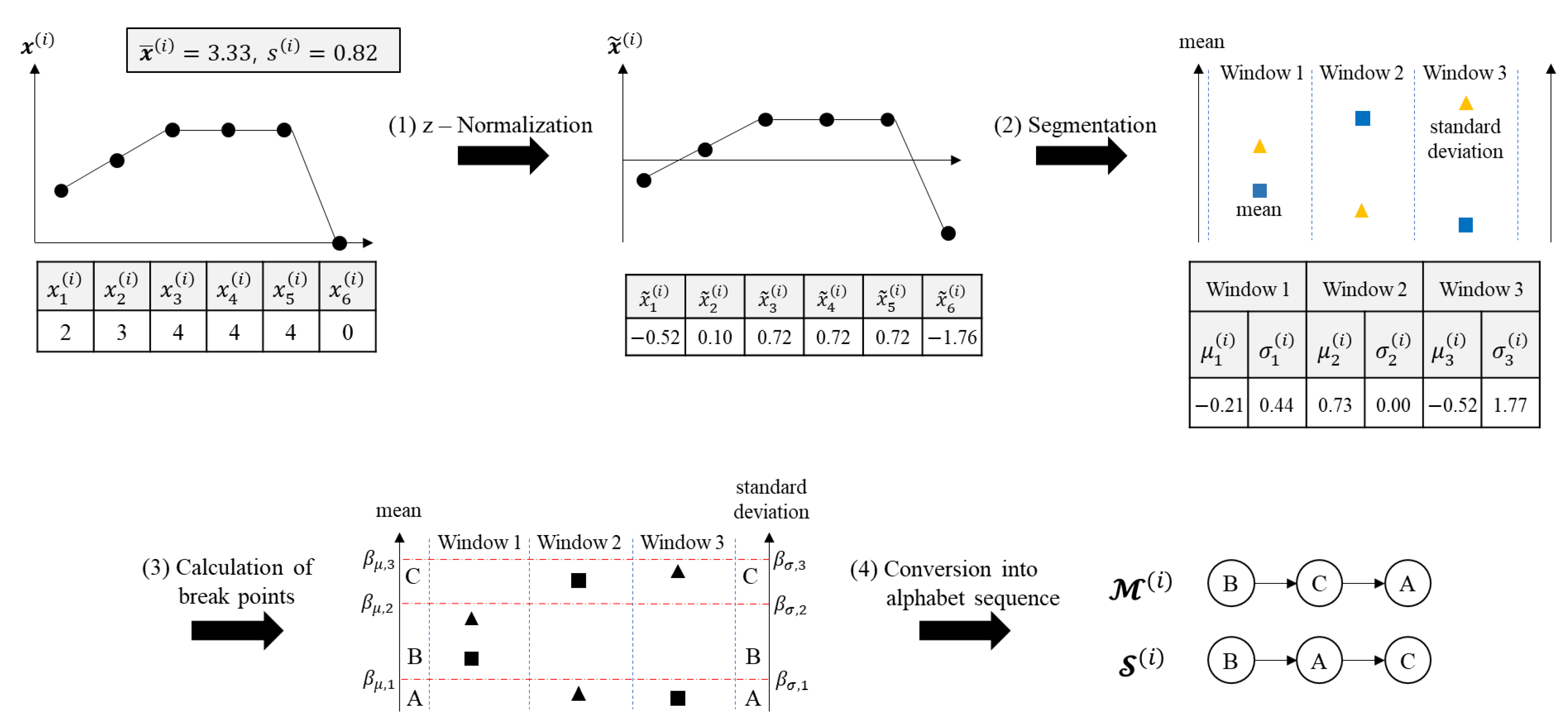
The objective of the preprocessing phase is to express ${\mathit{x}}^{\left(i\right)}$ as a tuple $\left({\mathbf{ℳ}}^{\left(i\right)},{\mathcal{S}}^{\left(i\right)}\right)$, where ${\mathbf{ℳ}}^{\left(i\right)}$ and ${\mathcal{S}}^{\left(i\right)}$ are window mean vector $i$ and window standard deviation vector $i$, respectively. The preprocessing phase consists of four steps: z-normalization, segmentation, calculation of break points, and conversion into an alphabetical sequence, as illustrated in Figure 2.

In the first step, ${\mathit{x}}^{\left(i\right)}$ for $i=1,2,\cdots ,n$ is normalized to ${\tilde{\mathit{x}}}^{\left(i\right)}$ with its mean ${\overline{x}}^{\left(i\right)}$ and standard deviation $s^{\left(i\right)}$ as:

$${\tilde{x}}_t^{\left(i\right)}=\frac{x_t^{\left(i\right)}-{\overline{x}}^{\left(i\right)}}{s^{\left(i\right)}}.$$

(3)

In the second step, ${\tilde{\mathit{x}}}^{\left(i\right)}$ for $i=1,2,\cdots ,n$ is split into $w$ windows, where $w$ is the number of windows set by the user, and the mean and standard deviation of each window are calculated by:

$${\mu }_j^{\left(i\right)}=\frac{{{\displaystyle \sum }}_{t=j\times n_{i,j}+1}^{\left(j+1\right)\times n_{i,j}}{\tilde{x}}_t^{\left(i\right)}}{n_{i,j}},$$

(4)

$${\sigma }_j^{\left(i\right)}=\sqrt{\frac{{{\displaystyle \sum }}_{t=j\times n_{i,j}+1}^{\left(j+1\right)\times n_{i,j}}{\left({\tilde{x}}_t^{\left(i\right)}-{\mu }_j^{\left(i\right)}\right)}^2}{n_{i,j}-1}},$$

(5)

where $n_{i,j}$ is the number of elements in the $j^{\mathrm{th}}\left(j=1,2,\cdots ,\mathrm{w}\right)$ window of ${\tilde{\mathit{x}}}^{\left(i\right)}$, which equals $T_i/w$ when $j\ne w$, and ${\tilde{\mathit{x}}}^{\left(i\right)}$ is expressed as a pair of vectors, one of window mean vector ${\mathbf{\mu }}^{\left(i\right)}=\left({\mu }_1^{\left(i\right)}, {\mu }_2^{\left(i\right)},\cdots ,{\mu }_w^{\left(i\right)}\right)$, and another of window standard deviation vector ${\mathbf{\sigma }}^{\left(i\right)}=\left({\sigma }_1^{\left(i\right)}, {\sigma }_2^{\left(i\right)},\cdots ,{\sigma }_w^{\left(i\right)}\right)$.

In the third step, break points ${\mathbf{\beta }}_{\mu }$ and ${\mathbf{\beta }}_{\sigma }$ for ${\mu }_j^{\left(i\right)}$ and ${\sigma }_j^{\left(i\right)}$ ($i=1,\cdots ,n,$, $j=1,\cdots ,w$), respectively, are obtained according to the size of the set of the alphabetical strings, $\left|\mathcal{A}\right|$, which is also the user parameter. As explained in Section 2.2, the break points ${\mathbf{\beta }}_{\mu }$ and ${\mathbf{\beta }}_{\sigma }$ are used as criterion to convert mean and standard deviation of each window into alphabets. ${\mathbf{\beta }}_{\mu }$ and ${\mathbf{\beta }}_{\sigma }$ are calculated and used not for individual samples but for all samples to consider the sample’s scale when generating new sample. The break point is obtained from $\mathrm{Pr}\left({\beta }_q\le x<{\beta }_{q+1}\right)=\frac{1}{\left|\mathcal{A}\right|}$, which implies that each interval $\left({\beta }_q, {\beta }_{q+1}\right]$, $q=1, 2, \cdots , \left|\mathcal{A}\right|-1$, contains the same number of values, and ${\beta }_q$ is therefore $\frac{q}{\left|\mathcal{A}\right|}\times 100\%$.

In the fourth step, ${\mathbf{\mu }}^{\left(i\right)}$ and ${\mathbf{\sigma }}^{\left(i\right)}$ are expressed as alphabetical sequences ${\mathbf{ℳ}}^{\left(i\right)}$ and ${\mathcal{S}}^{\left(i\right)}$, respectively, as follows:

$${ℳ}_j^{\left(i\right)}=\{\begin{array}{cc}\begin{array}{c}{\mathcal{A}}_{\mu , 1},\\ {\mathcal{A}}_{\mu , 2},\end{array}& \begin{array}{c} {\beta }_{\mu , 0}<{\mu }_j^{\left(i\right)}\le {\beta }_{\mu , 1}\\ {\beta }_{\mu , 1}<{\mu }_j^{\left(i\right)}\le {\beta }_{\mu , 2}\end{array}\\ \begin{array}{c}⋮\\ {\mathcal{A}}_{\mu , \left|{\mathcal{A}}_{\mu }\right|},\end{array}& \begin{array}{c}⋮\\ {\beta }_{\mu ,\left|{\mathcal{A}}_{\mu }\right|-1}<{\mu }_j^{\left(i\right)}\le {\beta }_{\mu ,\left|{\mathcal{A}}_{\mu }\right|}\end{array}\end{array},$$

(6)

$${\mathcal{S}}_j^{\left(i\right)}=\{\begin{array}{cc}\begin{array}{c}{\mathcal{A}}_{\sigma ,1},\\ {\mathcal{A}}_{\sigma ,2},\end{array}& \begin{array}{c} {\beta }_{\sigma , 0}<{\sigma }_j^{\left(i\right)}\le {\beta }_{\sigma , 1}\\ {\beta }_{\sigma , 1}<{\sigma }_j^{\left(i\right)}\le {\beta }_{\sigma , 2}\end{array}\\ \begin{array}{c}⋮\\ {\mathcal{A}}_{\sigma ,\left|{\mathcal{A}}_{\mu }\right|},\end{array}& \begin{array}{c}⋮\\ {\beta }_{\sigma , \left|{\mathcal{A}}_{\sigma }\right|-1}<{\sigma }_j^{\left(i\right)}\le {\beta }_{\sigma , \left|{\mathcal{A}}_{\sigma }\right|}\end{array}\end{array},$$

(7)

where ${\beta }_{\mu , 0}$ and ${\beta }_{\sigma , 0}$ are negative infinity, and ${\mathcal{A}}_{\mu ,j}$ and ${\mathcal{A}}_{\sigma ,j}$ indicate the $j^{\mathrm{th}}$ predefined alphabet (e.g., ${\mathcal{A}}_{\mu ,1}=\mathbb{A}$, ${\mathcal{A}}_{\sigma ,4}=𝕕$) for the window mean and standard deviation, respectively.

The first phase is summarized in Algorithm A1 in the Appendix A.

3.2. Generating Alphabetical Sequences

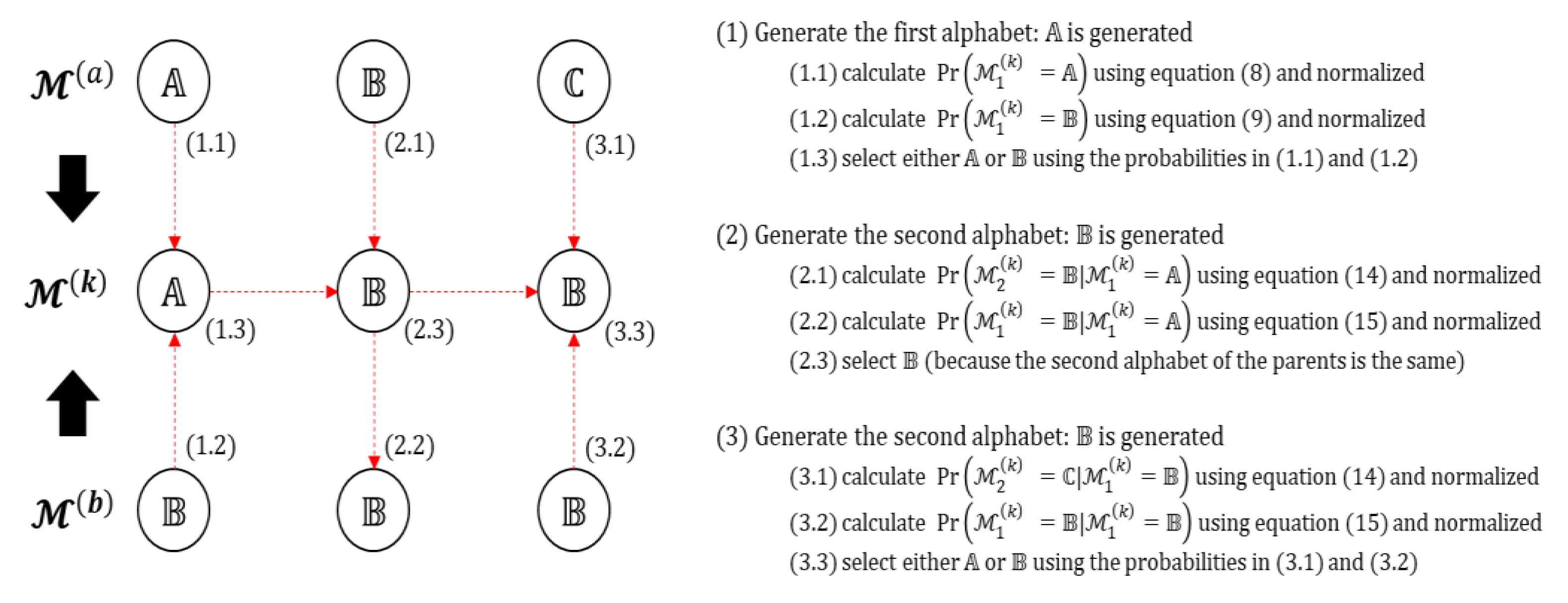
The second phase is to generate artificial sequences of alphabets for ${\mathbf{ℳ}}^{\left(k\right)}$ and ${\mathcal{S}}^{\left(k\right)}$ on the basis of two randomly selected parental samples $\left({\mathbf{ℳ}}^{\left(a\right)},{\mathcal{S}}^{\left(a\right)}\right)$ and $\left({\mathbf{ℳ}}^{\left(b\right)},{\mathcal{S}}^{\left(b\right)}\right)$. Figure 3 illustrates an example of the generating process of alphabetical sequence ${\mathbf{ℳ}}^{\left(k\right)}$ based on ${\mathbf{ℳ}}^{\left(a\right)}=\mathbb{A}\mathbb{B}ℂ\mathbb{B}$ and ${\mathbf{ℳ}}^{\left(b\right)}=\mathbb{B}\mathbb{B}\mathbb{B}ℂ$. Note that generating process of ${\mathcal{S}}^{\left(k\right)}$ is the same as the process of ${\mathbf{ℳ}}^{\left(k\right)}$.

In this figure, an edge from alphabet A to B denotes that alphabet A impacts on generating alphabet B.

Sequence ${\mathbf{ℳ}}^{\left(k\right)}$ for the window mean is generated by sequentially selecting an element from either ${ℳ}_j^{\left(a\right)}$ and ${ℳ}_j^{\left(b\right)}$ on the basis of the probabilities $\mathrm{Pr}\left({ℳ}_j^{\left(a\right)}|{\mathbf{ℳ}}_{1:j-1}^{\left(k\right)}\right)$ and $\mathrm{Pr}\left({ℳ}_j^{\left(b\right)}|{\mathbf{ℳ}}_{1:j-1}^{\left(k\right)}\right)$, where ${\mathbf{ℳ}}_{1:j-1}^{\left(k\right)}=\left({ℳ}_1^{\left(k\right)}, {ℳ}_2^{\left(k\right)}, \cdots ,{ℳ}_{j-1}^{\left(k\right)}\right)$ is a partial sequence of ${\mathbf{ℳ}}^{\left(k\right)}$. Sequence ${\mathcal{S}}^{\left(k\right)}$ for the window standard deviation is similarly generated on the basis of $\mathrm{Pr}\left({\mathcal{S}}_j^{\left(a\right)}|{\mathcal{S}}_{1:j-1}^{\left(k\right)}\right)$ and $\mathrm{Pr}\left({\mathcal{S}}_j^{\left(a\right)}|{\mathcal{S}}_{1:j-1}^{\left(k\right)}\right)$. ${\mathbf{ℳ}}^{\left(k\right)}$ and ${\mathcal{S}}^{\left(k\right)}$ are assumed to be independent of each other for simplicity.

Probabilities $\mathrm{Pr}\left({ℳ}_1^{\left(a\right)}\right)$ and $\mathrm{Pr}\left({ℳ}_1^{\left(b\right)}\right)$, which are used to select the first element ${ℳ}_1^{\left(k\right)}$, can be calculated by:

$$\mathrm{Pr}\left({ℳ}_1^{\left(a\right)}\right)=\frac{{{\displaystyle \sum }}_{i=1}^{n}I\left({ℳ}_1^{\left(i\right)}={ℳ}_1^{\left(a\right)}\right)+\alpha }{n+\alpha \times \left|{\mathcal{A}}_{\mu }\right|} ,$$

(8)

$$\mathrm{Pr}\left({ℳ}_1^{\left(b\right)}\right)=\frac{{{\displaystyle \sum }}_{i=1}^{n}I\left({ℳ}_1^{\left(i\right)}={ℳ}_1^{\left(b\right)}\right)+\alpha }{n+\alpha \times \left|{\mathcal{A}}_{\mu }\right|},$$

(9)

where $I\left(condition\right)$ is an indicator function, which returns 1 if $condition$ is satisfied, and 0, otherwise, and $\alpha \ge 0$ is a Laplace smoothing parameter to prevent $\mathrm{Pr}\left({ℳ}_1^{\left(a\right)}\right)$ and $\mathrm{Pr}\left({ℳ}_1^{\left(b\right)}\right)$ from becoming either zero or one. That is, $\mathrm{Pr}\left({ℳ}_1^{\left(a\right)}\right)$ and $\mathrm{Pr}\left({ℳ}_1^{\left(b\right)}\right)$ are calculated as smoothed ratio of ${ℳ}_1^{\left(a\right)}$ and ${ℳ}_1^{\left(b\right)}$ among the first alphabets of mean sequences, respectively.

Because ${ℳ}_1^{\left(a\right)}$ and ${ℳ}_1^{\left(a\right)}$ are selected with probabilities in (8) and (9), respectively, these probabilities should be normalized by dividing each by their sum as presented in Equations (10) and (11):

$$\widetilde{\mathrm{Pr}}\left({ℳ}_1^{\left(a\right)}\right)=\frac{\mathrm{Pr}\left({ℳ}_1^{\left(a\right)}\right)}{\mathrm{Pr}\left({ℳ}_1^{\left(a\right)}\right)+\mathrm{Pr}\left({ℳ}_1^{\left(b\right)}\right)} ,$$

(10)

$$\widetilde{\mathrm{Pr}}\left({ℳ}_1^{\left(b\right)}\right)=\frac{\mathrm{Pr}\left({ℳ}_1^{\left(b\right)}\right)}{\mathrm{Pr}\left({ℳ}_1^{\left(a\right)}\right)+\mathrm{Pr}\left({ℳ}_1^{\left(b\right)}\right)}$$

(11)

Probabilities, $\mathrm{Pr}\left({ℳ}_j^{\left(a\right)}|{\mathbf{ℳ}}_{1:j-1}^{\left(k\right)}\right)$ and $\mathrm{Pr}\left({ℳ}_j^{\left(b\right)}|{\mathbf{ℳ}}_{1:j-1}^{\left(k\right)}\right)$, used to select the $j^{\mathrm{th}} \left(2\le j\le w\right)$ element ${ℳ}_j^{\left(k\right)}$, can be calculated using the Markovian assumption:

$$\mathrm{Pr}\left({ℳ}_j^{\left(a\right)}|{\mathbf{ℳ}}_{1:j-1}^{\left(k\right)}\right)=\mathrm{Pr}\left({ℳ}_j^{\left(a\right)}|{ℳ}_{j-1}^{\left(k\right)}\right),$$

(12)

$$\mathrm{Pr}\left({ℳ}_j^{\left(b\right)}|{\mathbf{ℳ}}_{1:j-1}^{\left(k\right)}\right)=\mathrm{Pr}\left({ℳ}_j^{\left(b\right)}|{ℳ}_{j-1}^{\left(k\right)}\right)$$

(13)

where $\mathrm{Pr}\left({ℳ}_j^{\left(a\right)}|{ℳ}_{j-1}^{\left(k\right)}\right)$ and $\mathrm{Pr}\left({ℳ}_j^{\left(b\right)}|{ℳ}_{j-1}^{\left(k\right)}\right)$ are calculated by:

$$\mathrm{Pr}\left({ℳ}_j^{\left(a\right)}|{ℳ}_{j-1}^{\left(k\right)}\right)=\frac{{{\displaystyle \sum }}_{i=1}^n{{\displaystyle \sum }}_{h=\max \left(0,j-L\right)}^{\min \left(w, j+L-1\right)}I\left(\left({ℳ}_h^{\left(i\right)}={ℳ}_{j-1}^{\left(k\right)}\right) and \left({ℳ}_{h+1}^{\left(i\right)}={ℳ}_j^{\left(a\right)}\right)\right)}{{{\displaystyle \sum }}_{i=1}^n{{\displaystyle \sum }}_{h=\max \left(0,j-L\right)}^{\min \left(w, j+L\right)}I\left({ℳ}_h^{\left(i\right)}={ℳ}_{j-1}^{\left(k\right)}\right)},$$

(14)

$$\mathrm{Pr}\left({ℳ}_j^{\left(b\right)}|{ℳ}_{j-1}^{\left(k\right)}\right)=\frac{{{\displaystyle \sum }}_{i=1}^n{{\displaystyle \sum }}_{h=\max \left(0,j-L\right)}^{\min \left(w, j+L-1\right)}I\left(\left({ℳ}_h^{\left(i\right)}={ℳ}_{j-1}^{\left(k\right)}\right) and \left({ℳ}_{h+1}^{\left(i\right)}={ℳ}_j^{\left(b\right)}\right)\right)}{{{\displaystyle \sum }}_{i=1}^n{{\displaystyle \sum }}_{h=\max \left(0,j-L\right)}^{\min \left(w, j+L\right)}I\left({ℳ}_h^{\left(i\right)}={ℳ}_{j-1}^{\left(k\right)}\right)}$$

(15)

In Equations (14) and (15), $L$ is a parameter to restrict the search space to determine the number of alphabets that match ${ℳ}_{j-1}^{\left(k\right)}$, ${ℳ}_j^{\left(a\right)}$, ${ℳ}_j^{\left(b\right)}$ in ${\mathbf{ℳ}}^{\left(i\right)}$ for all values of $i$. The parent sample is randomly selected, and to produce the next sample, we adopt the Markov process for randomness and variability. In the Markov assumption, we can add more variability by properly setting the value of $L$ representing the size of the search space (Equations (14) and (15)). These probabilities should be normalized as follows:

$$\widetilde{\mathrm{Pr}}\left({ℳ}_j^{\left(a\right)}|{\mathbf{ℳ}}_{1:j-1}^{\left(k\right)}\right)=\frac{\mathrm{Pr}\left({ℳ}_j^{\left(a\right)}|{ℳ}_{j-1}^{\left(k\right)}\right)}{\mathrm{Pr}\left({ℳ}_j^{\left(a\right)}|{ℳ}_{j-1}^{\left(k\right)}\right)+\mathrm{Pr}\left({ℳ}_j^{\left(b\right)}|{ℳ}_{j-1}^{\left(k\right)}\right)}$$

(16)

$$\widetilde{\mathrm{Pr}}\left({ℳ}_j^{\left(b\right)}|{\mathbf{ℳ}}_{1:j-1}^{\left(k\right)}\right)=\frac{\mathrm{Pr}\left({ℳ}_j^{\left(b\right)}|{ℳ}_{j-1}^{\left(k\right)}\right)}{\mathrm{Pr}\left({ℳ}_j^{\left(a\right)}|{ℳ}_{j-1}^{\left(k\right)}\right)+\mathrm{Pr}\left({ℳ}_j^{\left(b\right)}|{ℳ}_{j-1}^{\left(k\right)}\right)}$$

(17)

An algorithm to generate alphabetical sequences of an artificial sample’s mean and standard deviation is presented as Algorithm A2. It is based on sampling from categorical distribution to select either $a$ or $b$. For example, the first element of ${\mathbf{ℳ}}^{\left(k\right)}$ follows the categorical distribution $\mathrm{C}\left({ℳ}_1^{\left(a\right)},{ℳ}_1^{\left(b\right)}|\widetilde{\mathrm{Pr}}\left({ℳ}_1^{\left(a\right)}\right),\widetilde{\mathrm{Pr}}\left({ℳ}_1^{\left(b\right)}\right)\right)$, implying that ${ℳ}_1^{\left(k\right)}$ is selected from ${ℳ}_1^{\left(a\right)}$ and ${ℳ}_1^{\left(b\right)}$ with probabilities $\widetilde{\mathrm{Pr}}\left({ℳ}_1^{\left(a\right)}\right)$ and $\widetilde{\mathrm{Pr}}\left({ℳ}_1^{\left(b\right)}\right)$.

3.3. Generating Time-Series Values

In this phase, time-series values ${\tilde{\mathbf{z}}}_j^{\left(k\right)}$ in window $j$ are generated from ${ℳ}_j^{\left(k\right)}$ and ${\mathcal{S}}_j^{\left(k\right)}$ for $j=1,2,\cdots ,w$. Let ${ℳ}_j^{\left(k\right)}$ be ${\mathcal{A}}_{\mu ,r_1}$ implying that ${\beta }_{\mu ,r_1-1}<{\mu }_j^{\left(k\right)}\le {\beta }_{\mu ,r_1}$, and ${\mathcal{S}}_j^{\left(k\right)}$ be ${\mathcal{A}}_{\mu ,r_2}$, implying that ${\beta }_{\sigma ,r_2-1}<{\sigma }_j^{\left(k\right)}\le {\beta }_{\sigma ,r_2}$. We assume that ${\tilde{\mathit{z}}}_j^{\left(k\right)}$ follows a normal distribution, with the mean ${\mu }_j^{\left(k\right)}$ and standard deviation ${\sigma }_j^{\left(k\right)}$, and ${\mu }_j^{\left(k\right)}$ and ${\sigma }_j^{\left(k\right)}$ uniformly distributed in $\left({\beta }_{\mu ,r_1-1},{\beta }_{\mu ,r_1}\right]$ and $\left({\beta }_{\sigma ,r_2-1},{\beta }_{\sigma ,r_2}\right]$, respectively, when $r_1$ and $r_2$ are not 1. When $r_1$ is 1, we set ${\mu }_j^{\left(k\right)}={\beta }_{\mu ,r_1}$, and ${\sigma }_j^{\left(k\right)}={\beta }_{\sigma ,r_2}$ when $r_2$ is 1. We also assume that the length of ${\tilde{\mathit{z}}}_j^{\left(k\right)}$ follows a uniform distribution in $\left[\min \left(\frac{T_a}{w},\frac{T_b}{w}\right),\max \left(\frac{T_a}{w},\frac{T_b}{w}\right)\right]$, where $a$ and $b$ are indices of the parents of $k$, and $\frac{T_a}{w}$ and $\frac{T_b}{w}$ denote the number of elements in each window of ${\tilde{\mathit{x}}}^{\left(a\right)}$ and ${\tilde{\mathit{x}}}^{\left(b\right)}$, respectively.

After a ${\tilde{\mathbf{z}}}_j^{\left(k\right)}$ for every value of $j$ is generated, it should be inversely transformed to ${\mathbf{z}}_j^{\left(k\right)}$ using its mean ${\overline{z}}^{\left(k\right)}$ and standard deviation $s^{\left(k\right)}$. We set them as a weighted average of ${\overline{x}}^{\left(a\right)}$ and ${\overline{x}}^{\left(b\right)}$, and $s^{\left(a\right)}$ and $s^{\left(b\right)}$, respectively, as presented Equations (18) and (19):

$${\overline{z}}^{\left(k\right)}=r\times {\overline{x}}^{\left(a\right)}+\left(1-r\right)\times {\overline{x}}^{\left(b\right)},$$

(18)

$$s^{\left(k\right)}=r\times s^{\left(a\right)}+\left(1-r\right)\times s^{\left(b\right)},$$

(19)

where $0<r<1$ is randomly chosen. That is, Equation (18) means ${\overline{z}}^{\left(k\right)}$ is randomly selected between ${\overline{x}}^{\left(a\right)}$ and ${\overline{x}}^{\left(b\right)}$, and Equation (19) means ${\mathrm{s}}^{\left(k\right)}$ is randomly selected between $s^{\left(a\right)}$ and $s^{\left(b\right)}$.

4. Numerical Example

This section describes an example of how a new time series ${\mathit{z}}^{\left(k\right)}$ is generated using the proposed method.

Table 3. Example original dataset.

Index	Data	Mean	Standard Deviation
1	(10, 10, 11, 11, 12, 13, 13, 14, 13, 13, 13, 14, 15, 14, 14, 15, 16, 16)	13.17	1.77
2	(10, 9, 9, 9, 10, 9, 10, 10, 10, 9, 9, 8, 9, 9, 8, 7, 7, 7)	8.83	1.01
3	(11, 11, 12, 13, 12, 12, 12, 11, 11, 11, 10, 9, 8, 9, 9, 10, 9, 10)	10.56	1.34
4	(9, 8, 9, 9, 9, 8, 9, 9, 9, 10, 11, 11, 11, 10, 10, 10, 9, 8)	9.39	0.95
5	(11, 11, 11, 12, 12, 12, 12, 13, 12, 11, 11, 12, 12, 13, 13, 14, 15, 15)	12.33	1.25

shows example dataset $\mathrm{X}$, which consists of five samples. Each sample is a time series collected from start to failure of a part by a sensor. In each sample, there are 18 numeric data, implying that life of each corresponding part is 18. Please note that the proposed method can be applied to the data that includes samples with different lengths.

Phase 1. Preprocessing

(1)

z-normalization

Each sample in Table 3 is normalized according to its mean and standard deviation as follows.

${\tilde{\mathit{x}}}^{\left(1\right)}=$ (−1.79, −1.79, −1.22, −1.22, −0.66, −0.09, −0.09, 0.47, −0.09, −0.09, −0.09, 0.47, 1.03, 0.47, 0.47, 1.03, 1.6, 1.6),

${\tilde{\mathit{x}}}^{\left(2\right)}=$ (1.15, 0.16, 0.16, 0.16, 1.15, 0.16, 1.15, 1.15, 1.15, 0.16, 0.16, −0.82, 0.16, 0.16, −0.82, −1.81, −1.81, −1.81),

${\tilde{\mathit{x}}}^{\left(3\right)}=$ (0.33, 0.33, 1.08, 1.82, 1.08, 1.08, 1.08, 0.33, 0.33, 0.33, −0.41, −1.16, −1.9, −1.16, −1.16, −0.41, −1.16, −0.41),

${\tilde{\mathit{x}}}^{\left(4\right)}=$ (−0.41, −1.46, −0.41, −0.41, −0.41, −1.46, −0.41, −0.41, −0.41, 0.64, 1.69, 1.69, 1.69, 0.64, 0.64, 0.64, −0.41, −1.46),

${\tilde{\mathit{x}}}^{\left(5\right)}=$ (−1.07, −1.07, −1.07, −0.27, −0.27, −0.27, −0.27, 0.53, −0.27, −1.07, −1.07, −0.27, −0.27, 0.53, 0.53, 1.34, 2.14, 2.14).

(2)

Segmentation

Each normalized sample is split into $w \left(w=6\right)$ windows, and the mean and standard deviation of each window are calculated. For example, the first window of ${\tilde{\mathit{x}}}^{\left(2\right)}$ is (1.15, 0.16, 0.16) and its mean and standard deviation ${\mu }_1^{\left(2\right)}$ and ${\sigma }_1^{\left(2\right)}$ are 0.49 and 0.47, respectively. Values for ${\mu }_j^{\left(i\right)}$ and ${\sigma }_j^{\left(i\right)}$ for all $i$ and $j$ are calculated as follows.

${\mathbf{\mu }}^{\left(1\right)}=$ (−1.60, −0.66, 0.10, 0.10, 0.66, 1.41), ${\mathbf{\sigma }}^{\left(1\right)}=$ (0.27, 0.46, 0.26, 0.26, 0.26, 0.27),

${\mathbf{\mu }}^{\left(2\right)}=$ (0.49, 0.49, 1.15, −0.17, −0.17, −1.81), ${\mathbf{\sigma }}^{\left(2\right)}=$ (0.47, 0.47, 0.00, 0.46, 0.46, 0.00),

${\mathbf{\mu }}^{\left(3\right)}=$ (0.58, 1.33, 0.58, −0.41, −1.41, −0.66), ${\mathbf{\sigma }}^{\left(3\right)}=$ (0.35, 0.35, 0.35, 0.61, 0.35, 0.35),

${\mathbf{\mu }}^{\left(4\right)}=$ (−0.76, −0.76, −0.41, 1.34, 0.99, −0.41), ${\mathbf{\sigma }}^{\left(4\right)}=$ (0.49, 0.49, 0.00, 0.49, 0.49, 0.86),

${\mathbf{\mu }}^{\left(5\right)}=$ (−1.07, −0.27, −0.00, −0.80, 0.26, 1.87), ${\mathbf{\sigma }}^{\left(5\right)}=$ (0.00, 0.00, 0.38, 0.38, 0.38, 0.38).

(3)

Calculation of break points

We set $\left|{\mathcal{A}}_{\mu }\right|=\left|{\mathcal{A}}_{\sigma }\right|=3$, and break points ${\beta }_{\mu , j}$ and ${\beta }_{\sigma , j}$ are those that divide the values of all values of ${\mu }_j^{\left(i\right)}$ and ${\sigma }_j^{\left(i\right)}$, respectively, into three equal parts. For example, ${\beta }_{\mu , 1}=-0.41$ is 1/3 quantile of {−1.60, −0.66, 0.10, 0.10, 0.66, 1.41, 0.49, 0.49, 1.15, −0.17, −0.17, −1.81, 0.58, 1.33, 0.58, −0.41, −1.41, −0.66, −0.76, −0.76, −0.41, 1.34, 0.99, −0.41, −1.07, −0.27, −0.00, −0.80, 0.26, 1.87}. In this manner, all break points can be calculated by:

${\mathbf{\beta }}_{\mathbf{\mu }}=\left({\beta }_{\mu ,1},{\beta }_{\mu ,2},{\beta }_{\mu ,3}\right)=$ (−0.41, 0.49, 1.87),

${\mathbf{\beta }}_{\mathbf{\sigma }}=\left({\beta }_{\sigma ,1},{\beta }_{\sigma ,2},{\beta }_{\sigma ,3}\right)=$ (0.32, 0.46, 0.86).

(4)

Conversion into an alphabetical sequence

On the basis of ${\mathbf{\beta }}_{\mathbf{\mu }}$ and ${\mathbf{\beta }}_{\mathbf{\sigma }}$, ${\mathbf{\mu }}^{\left(i\right)}$ and ${\mathbf{\sigma }}^{\left(i\right)}$ are converted to an alphabetical sequence ${\mathbf{ℳ}}^{\left(i\right)}$ and ${\mathcal{S}}^{\left(i\right)}$ for all $i$, respectively. For example, ${\mu }_1^{\left(1\right)}=-1.60$ is converted as alphabet $\mathbb{A}$ because ${\beta }_{\mu , 0}=-\infty <-1.60<{\beta }_{\mu , 1}$, and ${\mu }_3^{\left(1\right)}=0.10$ is converted as alphabet $\mathbb{B}$ because ${\beta }_{\mu , 1}<0.10<{\beta }_{\mu , 2}$. Thus, ${\mu }^{\left(1\right)}=$ (−1.60, −0.66, 0.10, 0.10, 0.66, 1.41) is converted as $\mathbb{A}\mathbb{A}\mathbb{B}\mathbb{B}ℂℂ$. ${\mathbf{ℳ}}^{\left(i\right)}$ and ${\mathcal{S}}^{\left(i\right)}$ for all $i$ are obtained as follows.

${\mathbf{ℳ}}^{\left(1\right)}$ = $\mathbb{A}\mathbb{A}\mathbb{B}\mathbb{B}ℂℂ$, ${\mathcal{S}}^{\left(1\right)}=𝕒𝕔𝕒𝕒𝕒𝕒$,

${\mathbf{ℳ}}^{\left(2\right)}$ = $ℂℂℂ\mathbb{B}\mathbb{B}\mathbb{A}$, ${\mathcal{S}}^{\left(2\right)}=𝕔𝕔𝕒𝕔𝕔𝕒$,

${\mathbf{ℳ}}^{\left(3\right)}$ = $ℂℂℂ\mathbb{B}\mathbb{A}\mathbb{A}$, ${\mathcal{S}}^{\left(3\right)}=𝕓𝕓𝕓𝕔𝕓𝕓$,

${\mathbf{ℳ}}^{\left(4\right)}$ = $\mathbb{A}\mathbb{A}\mathbb{B}ℂℂ\mathbb{B}$, ${\mathcal{S}}^{\left(4\right)}=𝕔𝕔𝕒𝕔𝕔𝕔$,

${\mathbf{ℳ}}^{\left(5\right)}$ = $\mathbb{A}\mathbb{B}\mathbb{B}\mathbb{A}\mathbb{B}ℂ$, ${\mathcal{S}}^{\left(5\right)}=𝕒𝕒𝕓𝕓𝕓𝕓$.

Phase 2. Generating an alphabetical sequence

Suppose sample 1 and 3 are randomly selected as parents. The first mean alphabetical strings of sample 1 and 3 are $\mathbb{A}$ and $ℂ$, and the first standard deviation alphabetical strings are $𝕒$ and $𝕓$. Thus, $\mathrm{Pr}\left(\mathbb{A}\right)$, $\mathrm{Pr}(ℂ)$, $\mathrm{Pr}(𝕒)$, and $\mathrm{Pr}(𝕓)$ should be calculated and normalized using Equations (6)–(9).

$$\mathrm{Pr}\left(\mathbb{A}\right)=\frac{3}{5},\mathrm{Pr}(ℂ)=\frac{2}{5},\widetilde{\mathrm{Pr}}\left(\mathbb{A}\right)=\frac{\frac{3}{5}}{\frac{3}{5}+\frac{2}{5}}=\frac{3}{5},\widetilde{\mathrm{Pr}}(ℂ)=\frac{\frac{2}{5}}{\frac{3}{5}+\frac{2}{5}}=\frac{2}{5}$$

$$\mathrm{Pr}(𝕒)=\frac{2}{5},\mathrm{Pr}(𝕓)=\frac{1}{5},\widetilde{\mathrm{Pr}}(𝕒)=\frac{\frac{2}{5}}{\frac{2}{5}+\frac{1}{5}}=\frac{2}{3},\widetilde{\mathrm{Pr}}(𝕓)=\frac{\frac{1}{5}}{\frac{2}{5}+\frac{1}{5}}=\frac{1}{3}$$

${ℳ}_1^{\left(k\right)}$ is sampling from $\mathrm{C}\left(\mathbb{A},ℂ|\frac{3}{5},\frac{2}{5}\right)$, and ${\mathcal{S}}_1^{\left(k\right)}$ is sampling from $\mathrm{C}\left(𝕓,𝕔|\frac{2}{3},\frac{1}{3}\right)$, and as a result, $\mathbb{A}$ and $𝕓$ are selected.

The second mean alphabets of sample 1 and 3 are $\mathbb{A}$ and $ℂ$, and the second standard deviation alphabets are $𝕔$ and $𝕓$. Therefore, $\mathrm{Pr}\left(\mathbb{A}|\mathbb{A}\right)$, $\mathrm{Pr}\left(ℂ|\mathbb{A}\right)$, $\mathrm{Pr}\left(𝕔|𝕒\right)$, and $\mathrm{Pr}\left(𝕓|𝕒\right)$ should be calculated and normalized using Equations (10)–(15). For convenience, we set $L$ to 1, and accordingly, ${\mathbf{ℳ}}_{1:3}^{\left(i\right)}$ and ${\mathcal{S}}_{1:3}^{\left(i\right)}$ for all $i$ were used for the calculation.

$$\mathrm{Pr}\left(\mathbb{A}|\mathbb{A}\right)=\frac{2}{3},\mathrm{Pr}\left(ℂ|\mathbb{A}\right)=\frac{0}{3},\widetilde{\mathrm{Pr}}\left(\mathbb{A}|\mathbb{A}\right)=\frac{\frac{2}{3}}{\frac{2}{3}+0}=1,\widetilde{\mathrm{Pr}}\left(ℂ|\mathbb{A}\right)=\frac{0}{\frac{2}{3}+0}=0$$

$$\mathrm{Pr}\left(𝕔|𝕒\right)=\frac{1}{3},\mathrm{Pr}\left(𝕓|𝕒\right)=\frac{1}{3},\widetilde{\mathrm{Pr}}\left(𝕔|𝕒\right)=\frac{\frac{1}{3}}{\frac{1}{3}+\frac{1}{3}}=\frac{1}{2},\widetilde{\mathrm{Pr}}\left(𝕓|𝕒\right)=\frac{\frac{1}{3}}{\frac{1}{3}+\frac{1}{3}}=\frac{1}{2}$$

${ℳ}_2^{\left(k\right)}$ is sampling from $\mathrm{C}\left(\mathbb{A},ℂ|1,0\right)$, and ${\mathcal{S}}_2^{\left(k\right)}$ is sampling from $\mathrm{C}\left(𝕓,𝕔|\frac{1}{2},\frac{1}{2}\right)$, and as a result, $\mathbb{A}$ and $𝕓$ are selected. This process repeats until $j$ becomes $w=6$.

From this phase, we obtain ${\mathbf{ℳ}}^{\left(k\right)}=\mathbb{A}\mathbb{A}\mathbb{B}ℂℂℂ$ and ${\mathcal{S}}^{\left(k\right)}=𝕒𝕓𝕓𝕓𝕓𝕔$.

Phase 3. Generating time-series values

In this phase, ${\tilde{\mathbf{z}}}_j^{\left(k\right)}$ are generated from ${ℳ}_j^{\left(k\right)}$ and ${\mathcal{S}}_j^{\left(k\right)}$ for $j=1, 2, \cdots , 6$, and we obtain ${\tilde{\mathbf{z}}}^{\left(k\right)}=$ (−0.6, −0.11, 0.16, −0.23, −1.32, −0.12, −0.04, 0.44, 0.66, 0.64, 1.23, 0.39, 0.88, 0.9, 1.86, 0.45, −0.2, 1.09).

The generation process for the first window $\left(j=1\right)$ is as follows. Since ${ℳ}_j^{\left(k\right)}=\mathbb{A}$ and ${\mathcal{S}}_j^{\left(k\right)}=𝕒$, $U\left[\min \left(\frac{T_1}{w}, \frac{T_3}{w}\right),\max \left(\frac{T_1}{w}, \frac{T_3}{w}\right)\right]=U\left[3, 3\right]=3$ samples are generated, where each sample follows a normal distribution with a mean ${\beta }_{\mu , 1}=-0.41$ and standard deviation ${\beta }_{\sigma , 1}=0.32$, because ${ℳ}_j^{\left(k\right)}$ and ${\mathcal{S}}_j^{\left(k\right)}$ are the first alphabets, and we use the constant mean and standard deviation. As a result, we obtain ${\tilde{\mathbf{z}}}_1^{\left(k\right)}=\left(-0.60,-0.11, 0.16\right)$. As an another example, for the fourth window ($j=4$), ${ℳ}_j^{\left(k\right)}=ℂ$ and ${\mathcal{S}}_j^{\left(k\right)}=𝕓$, and three samples are generated if each sample follows a normal distribution with a mean in $U[{\beta }_{\mu ,1}=-0.41,{\beta }_{\mu , 2}=0.49$] and standard deviation $\sigma$ in $U[{\beta }_{\sigma , 2}=$0.32, ${\beta }_{\sigma , 3}=$0.46]. As a result, we obtain ${\tilde{\mathbf{z}}}_4^{\left(k\right)}=\left(0.88, 0.90, 1.86\right)$.

Finally, ${\mathbf{z}}^{\left(k\right)}$ is obtained by inversely transforming ${\tilde{z}}_j^{\left(k\right)}$ with ${\overline{z}}^{\left(k\right)}=0.65\times {\overline{x}}^{\left(1\right)}+\left(1-0.65\right)\times {\overline{x}}^{\left(3\right)}=12.25$ and $s^{\left(k\right)}=0.82\times s^{\left(1\right)}+\left(1-0.18\right)\times s^{\left(3\right)}=1.42$, where $r=0.65$ and 0.18 are randomly chosen weights.

${\mathbf{z}}^{\left(k\right)}=$ (11.4, 12.1, 12.48, 11.93, 10.38, 12.08, 12.2, 12.88, 13.19, 13.16, 14.00, 12.81, 13.5, 13.53, 14.89, 12.89, 11.97, 13.80).

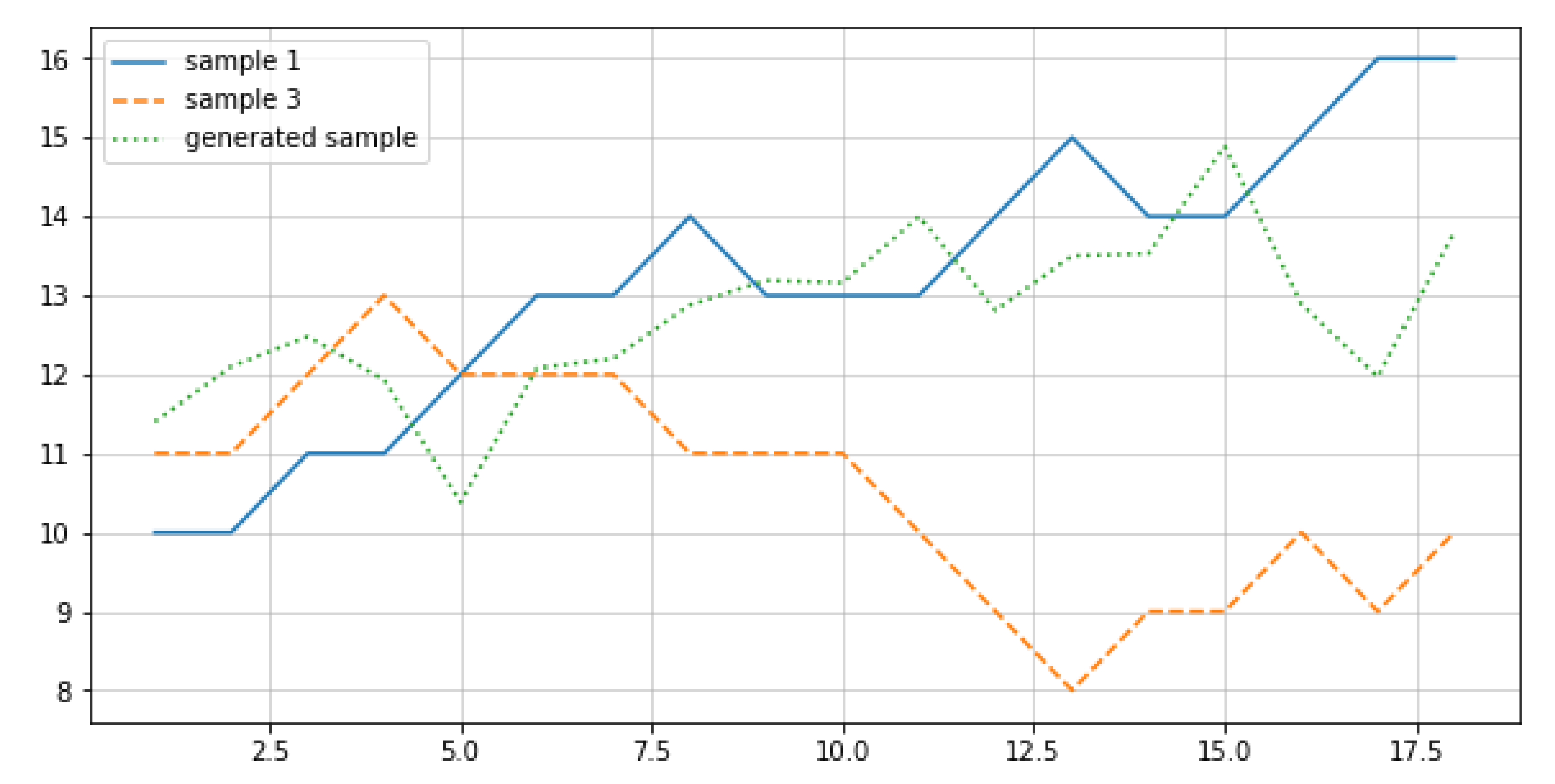
Figure 4 shows the generated sample and its parents (sample 1 and 3) of the example. Dashed and dotted lines denote samples 1 and 3 in Table 3, respectively, and solid line denotes the generated sample when the parents are the sample 1 and 3. Y-axis denotes the sensor value and X-axis denotes time, and thus the horizontal length of a line indicates the whole life. As explained before, the length (i.e., whole life) of every sample in X is 18, and thus the length of the generated sample is also 18. To be more accurate, the length of the generated sample follows uniform distribution with [minimum length of parents, maximum length of parents].

As seen in this graph, the generated sample follows a similar pattern to the ones of sample 1 and 3, which implies it contains the characteristics of exiting samples. However, at the same time, the generated sample should not be too close to the exiting samples in order to ensure the variability. The proposed method selects two parent samples at random, and all alphabet sequences are created on the basis of the Equations (12)–(17), which ensure enough randomness and variability of the generated samples when, e.g., selecting time series size for each alphabet, selecting the first alphabet, and so forth.

5. Experiment and Results

In this section, we describe an experiment to verify that the samples generated by the proposed method contribute to training an RUL model without overfitting. Two RUL prediction models were compared in terms of mean absolute percent error (MAPE), one with an original dataset $\mathrm{X}$ and the other with a dataset $\mathrm{X}{{\displaystyle \cup }}^{\text{}}\mathrm{Z}$, where $\mathrm{Z}$ is an artificially generated dataset. Section 5.1 explains the procedure of the experiment, Section 5.2 introduces the datasets and hyperparameters used in the experiment, and Section 5.3 shows the results.

5.1. Procedure

First, an original sample $i$, ${\mathit{x}}^{\left(i\right)}$ is reserved for the test, and the others (i.e., ${\mathrm{X}}^{\left(-i\right)}\equiv \mathrm{X}-\left\{{\mathit{x}}^{\left(i\right)}\right\}$) are used for training. Second, an RUL prediction model $f_1$ is trained with ${\mathrm{X}}^{\left(-i\right)}$, to which the transformation for RUL prediction is applied, ${{\displaystyle \bigcup }}_{\mathit{x}\in {\mathrm{X}}^{\left(-i\right)}}^{ }D\left(\mathit{x}\right)$. Third, the MAPE of the model for $D\left({\mathit{x}}^{\left(i\right)}\right)$, $MAP{E}_{1,i}$ is calculated. Fourth, we repeat $Q=100$ times to generate $Z=\left\{{\mathbf{z}}^{\left(k\right)}|k=1, 2, \cdots ,n-1\right\}$ using the proposed algorithm for ${\mathrm{X}}^{\left(-i\right)}$ under hyperparameters $w$, $L$, $\left|{\mathcal{A}}_{\mu }\right|$, and $\left|{\mathcal{A}}_{\sigma }\right|$; train $f_2$ with ${{\displaystyle \bigcup }}_{\mathit{x}\in {\mathrm{X}}^{\left(-i\right)}{{\displaystyle \cup }}^{\text{}}Z}^{ }D\left(\mathit{x}\right)$; and then calculate $MAP{E}_{2,i}^{\left(q\right)}$. Finally, $MAP{E}_{1,i}$ and the mean of 〖$MAP{E}_{2,i}^{\left(q\right)}$ are compared. This procedure is repeated for all possible values of $i$, $w$, $L$, $\left|{\mathcal{A}}_{\mu }\right|$, $\left|{\mathcal{A}}_{\sigma }\right|$, and the models.

The specific procedure is described in Algorithm A3 and the flowchart to illustrate to calculate $MAP{E}_{1,i}$, and $MAP{E}_{2,i}$ is presented in Figure 5.

In Step 6 and Step 7 of this algorithm, MAPE is calculated by:

$$MAPE=\frac{1}{T_i\times 0.7-T_i\times 0.3}\times {{\displaystyle \sum }}_{t=T_i\times 0.3}^{T_i\times 0.7}\left|\frac{y_t^{\left(i\right)}-f\left(\mathbf{\varphi }\left({\mathit{x}}_{1:t}^{\left(i\right)}\right)\right)}{y_t^{\left(i\right)}}\right|$$

(20)

This figure illustrates an example of the procedure to calculate $MAP{E}_{1,4}$ and $MAP{E}_{2,4}$. The specific process illustrated in this figure is as follows:

(1)

${\mathit{x}}^{\left(1\right)}$,${\mathit{x}}^{\left(2\right)}$,${\mathit{x}}^{\left(3\right)}$, and ${\mathit{x}}^{\left(4\right)}$ are transformed into $D\left({\mathit{x}}^{\left(1\right)}\right)$, $D\left({\mathit{x}}^{\left(2\right)}\right)$, $D\left({\mathit{x}}^{\left(3\right)}\right)$, and $D\left({\mathit{x}}^{\left(4\right)}\right)$ by applying feature functions, respectively.

(2)

RUL prediction model, $f_1$, is trained with $D\left({\mathit{x}}^{\left(1\right)}\right){{\displaystyle \cup }}^{\text{}}D\left({\mathit{x}}^{\left(2\right)}\right){{\displaystyle \cup }}^{\text{}}D\left({\mathit{x}}^{\left(3\right)}\right)$.

(3)

$D\left({\mathit{x}}^{\left(4\right)}\right)$ is used to validate $f_1$. That is, ${\widehat{y}}_t{}^{\left(4\right)}=f_1\left(\mathbf{\varphi }\left({\mathit{x}}_{1:t}^{\left(4\right)}\right)\right)$ for all $t$ is obtained and the prediction results are used to calculate $MAP{E}_{1,4}$.

(4)

Three new samples, ${\mathbf{z}}^{\left(1\right)}$, ${\mathbf{z}}^{\left(2\right)}$, and ${\mathbf{z}}^{\left(3\right)}$, are generated by means of the proposed method.

(5)

${\mathbf{z}}^{\left(1\right)}$,${\mathbf{z}}^{\left(2\right)}$, and ${\mathbf{z}}^{\left(3\right)}$ are also transformed into $D\left({\mathbf{z}}^{\left(1\right)}\right)$, $D\left({\mathbf{z}}^{\left(2\right)}\right)$, and $D\left({\mathbf{z}}^{\left(3\right)}\right)$.

(6)

RUL prediction model, $f_2$ is trained with $D\left({\mathit{x}}^{\left(1\right)}\right){{\displaystyle \cup }}^{\text{}}D\left({\mathit{x}}^{\left(2\right)}\right){{\displaystyle \cup }}^{\text{}}D\left({\mathit{x}}^{\left(3\right)}\right){{\displaystyle \cup }}^{\text{}}D\left({\mathbf{z}}^{\left(1\right)}\right){{\displaystyle \cup }}^{\text{}}D\left({\mathbf{z}}^{\left(2\right)}\right){{\displaystyle \cup }}^{\text{}}D\left({\mathbf{z}}^{\left(3\right)}\right)$.

(7)

$D\left({\mathit{x}}^{\left(4\right)}\right)$ is used to validate $f_2$. That is, ${\widehat{y}}_t{}^{\left(4\right)}=f_2\left(\mathbf{\varphi }\left({\mathit{x}}_{1:t}^{\left(4\right)}\right)\right)$ for all $t$ is obtained, and the prediction results are used to calculate $MAP{E}_{2,4}$.

5.2. Experiment Setting

Datasets were obtained from the prognostic data repository of the U.S. National Aeronautics and Space Administration.

Table 4. Used datasets.

Dataset	Feature	Number of Samples	Mean Length	Reference
Battery #1	Capacity	4	159.00	[30]
Battery #6	Capacity	4	90.75
FEMTO Bearing Set #1	Vibration signal	4	44,154,880.00	[31]

shows information of the datasets.

All three datasets are well known and have been widely used in the literature for the purpose of verifying the performance of the developed machine learning methods. Each sample in the first and second dataset is a time series of the capacity of lithium-ion battery until it is dead. Discharge was carried out at 24 °C, and each battery was regarded as dead when its capacity was at 30%. Each sample of the third dataset was a signal from vibration sensor attached to bearing. The operating condition of the bearing was 1800 rpm and 4000N, and sampling frequency of the sensor was 25.6 kHz.

Hyperparameters for each experiment are given in the following

Table 5. Hyper parameters for each experiment.

Dataset	Model	$\mathit{w}$	$\mathit{L}$	$\left|{\mathcal{A}}_{\mathit{\mu }}\right|$	$\left|{\mathcal{A}}_{\mathit{\sigma }}\right|$	$\mathit{\varphi }$
Battery	MLP (5, 5) LSTM (10, 5, 32, 50) SVR (1, 0.1, rbf)	50	3	3	3	Cumulative RMS and kurtosis
Bearing	MLP (10, 10) LSTM (20, 10, 32, 50) SVR (1, 0.1, rbf)	10000	6	4	4

.

Battery: Battery #1 and #6; bearing: FEMTO Bearing Set #1; MLP($h_1$, $h_2$): multi-layered perceptron with two hidden layers with $h_1$ and $h_2$ nodes, respectively; LSTM($h$, $s$, $b$, $e$): long short-term memory with $h$ neurons, $s$ timestamps, $b$ batch size, and $e$ epochs; SVR($C$, $\epsilon$, $\kappa$): support vector regression with regularization parameter $C$, epsilon $\epsilon$, and kernel function $\kappa$.

5.3. Results

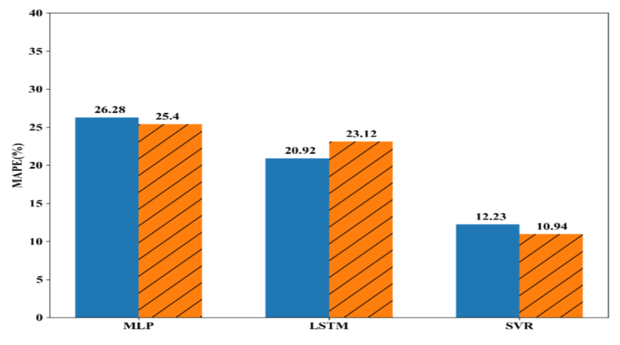
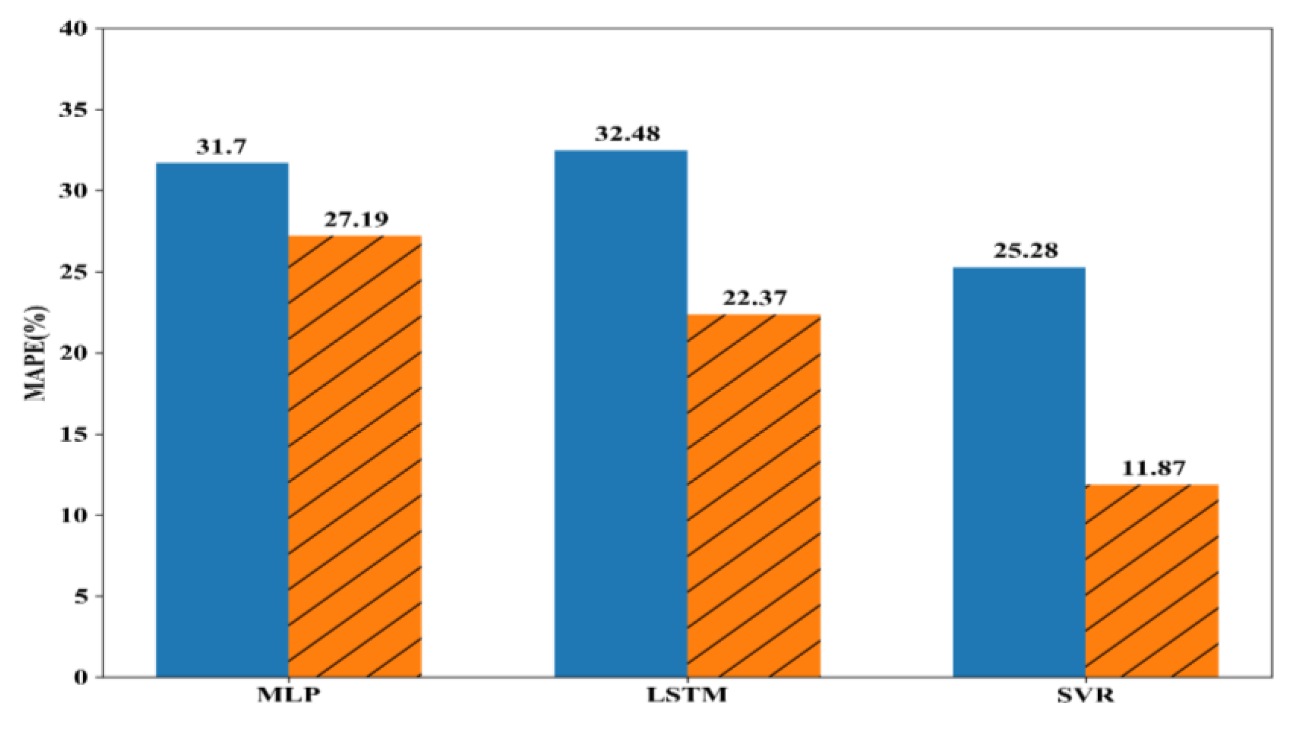
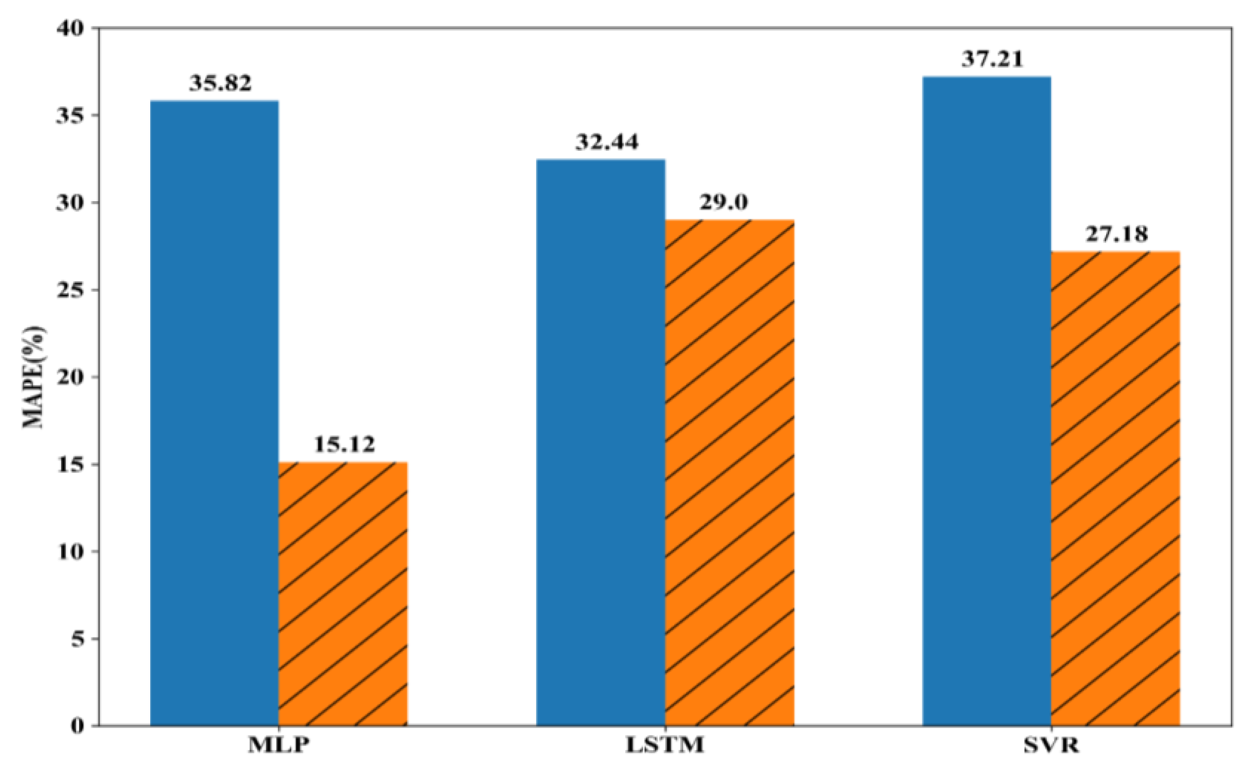
Figure 6, Figure 7 and Figure 8 show the experiment results with battery #1, battery #6, and bearing datasets. In the figures, blue bars denote the MAPEs of the model trained with original samples except for the test sample, and the orange bars denote the MAPEs of a model trained with original samples and generated samples.

From the results presented in Figure 6, Figure 7 and Figure 8, we found the following. First, when we included the generated samples for training, except for the LSTM with battery #1 as shown in Figure 6, the MAPEs were smaller than those of cases with only original samples. In the case of MLP with bearing, shown in Figure 8, 20.6% of MAPE was decreased, which was the largest improvement. This shows the proposed method to artificially generate the training samples is effective and could be used to improve the performance of models. Second, MAPE of the model trained using original samples without test sample could be very high. For example, MAPEs of MLP and SVR for the bearing dataset were 35.82% and 37.21%, respectively. This may have been because the features of some test samples (i.e., cumulative root mean square and kurtosis) are quite different from those of the other samples. In other words, the relationships between feature vectors and label (i.e., RUL) are markedly different from each other. In this case, the proposed method effectively decreased the MAPE, as in the case of the MLP for the bearing dataset. Third, the proposed method showed bigger MAPE when using LSTM for battery #1 (Figure 6), contrary to the other results. In essence, LSTM considered previous feature values (i.e., cumulative RMS and kurtosis at time $\mathrm{t}-1$) to predict the current label (i.e., RUL at t), but the proposed method did not consider the relationship between two consecutive values. Instead, it took the relationship between two consecutive windows into the consideration, and the values within a window were aggregated to single value, either mean or standard deviation. We think this sometimes may worsen the performance of the model when using more samples for training, which, in turn, results in the larger value of MAPE. However, we obtained smaller MAPEs in battery #6 and bearing, as shown in Figure 7 and Figure 8.

From the experiment, we verified that the proposed method can solve the data insufficiency problem that is common for RUL prediction and often leads to overfitting. In other words, the RUL prediction model trained with original samples and generated samples is more generalized than the one trained with original samples only.

6. Conclusions

Due to time and cost, it is often difficult to collect sufficient run-to-failure data to train ML- and DL-based RUL models. The data insufficiency problem can result in overfitting and undermining of a model’s performance. In this paper, we proposed a time-series data-generation method that identifies patterns from alphabetical sequences converted from original time-series samples using SAX and generates new sequence on the basis of these patterns. Finally, it generates time-series values from each alphabet in the generated sequence. In an experiment using three benchmark datasets, we found that the samples generated by the proposed method effectively increased the performance of the RUL prediction model.

Future efforts to improve the proposed method should take into the account the relationship between consecutive values when generating time-series values. In addition, the proposed method was designed for a univariate time series and may be not appropriate for multivariate time series, which are common in datasets used for RUL predictions. The proposed method should therefore be expanded to consider multivariate time series. Finally, the proposed method has many parameters such as the number of windows, alphabets, and generated samples, which would impact the prediction performance of RUL prediction model. Thus, in the future research, sensitivity analysis of the parameters should be conducted and the method to choose the proper parameter values should be developed.

References

- Xia, T.; Dong, Y.; Xiao, L.; Du, S.; Pan, E.; Xi, L. Recent advances in prognostics and health management for advanced manufacturing paradigms. Reliab. Eng. Syst. Saf. 2018, 178, 255–268. [Google Scholar] [CrossRef]
- Ahmad, R.; Kamaruddin, S. An overview of time-based and condition-based maintenance in industrial application. Comput. Ind. Eng. 2012, 63, 135–149. [Google Scholar] [CrossRef]
- Si, X.S.; Wang, W.; Hu, C.H.; Zhou, D.H. Remaining useful life estimation–a review on the statistical data driven approaches. Eur. J. Oper. Res. 2011, 213, 1–14. [Google Scholar] [CrossRef]
- Okoh, C.; Roy, R.; Mehnen, J.; Redding, L. Overview of remaining useful life prediction techniques in through-life engineering services. Procedia Cirp 2014, 16, 158–163. [Google Scholar] [CrossRef] [Green Version]
- Zhu, J.; Yang, Z. Themo-elasto-plastic stress and strain analysis and life prediction of gas turbine. Proc. Int. Conf. Meas. Technol. Mechatron. Autom. 2010, 1019–1022. [Google Scholar]
- Taheri, M.J.; Taheri, P. Feasibility study of congeneration for a gas power plant. In Proceedings of the 2017 IEEE Electrical Power and Energy Conference, Saskatoon, SK, Canada, 22–25 October 2017. [Google Scholar]
- Liao, L.; Köttig, F. Review of hybrid prognostics approaches for remaining useful life prediction of engineered systems, and an application to battery life prediction. IEEE Trans. Reliab. 2014, 63, 191–207. [Google Scholar] [CrossRef]
- Lyu, Y.; Gao, J.; Chen, C.; Jiang, Y.; Li, H.; Chen, K.; Zhang, Y. Joint model for residual life estimation based on Long-Short Term Memory network. Neurocomputing 2020, 410, 284–294. [Google Scholar] [CrossRef]
- Ruiz-Tagle Palazuelos, A.; Droguett, E.L.; Pascual, R. A novel deep capsule neural network for remaining useful life estimation. Proceedings of the Institution of Mechanical Engineers. Part O J. Risk Reliab. 2020, 234, 151–167. [Google Scholar]
- Sun, H.; Zhang, J.; Mo, R.; Zhang, X. In-process tool condition forecasting based on a deep learning method. Robot. Comput. Integr. Manuf. 2020, 64, 101924. [Google Scholar] [CrossRef]
- Mo, Y.; Wu, Q.; Li, X.; Huang, B. Remaining useful life estimation via transformer encoder enhanced by a gated convolutional unit. J. Intell. Manuf. 2021, 1–10. [Google Scholar] [CrossRef]
- An, D.; Choi, J.H.; Kim, N.H. Prediction of remaining useful life under different conditions using accelerated life testing data. J. Mech. Sci. Technol. 2018, 32, 2497–2507. [Google Scholar] [CrossRef]
- Borst, N.G. Adaptations for CNN-LSTM Network for Remaining Useful Life Prediction: Adaptable Time Window and Sub-Network Training. Master’s Thesis, Delft University of Technology, Delft, The Netherlands, August 2020. [Google Scholar]
- Xie, Z.; Du, S.; Lv, J.; Deng, Y.; Jia, S. A Hybrid Prognostics Deep Learning Model for Remaining Useful Life Prediction. Electronics 2021, 10, 39. [Google Scholar] [CrossRef]
- Ramasso, E.; Gouriveau, R. Remaining useful life estimation by classification of predictions based on a neuro-fuzzy system and theory of belief functions. IEEE Trans. Reliab. 2014, 63, 555–566. [Google Scholar] [CrossRef]
- Huang, S.; Guo, Y.; Liu, D.; Zha, S.; Fang, W. A two-stage transfer learning-based deep learning approach for production progress prediction in iot-enabled manufacturing. IEEE Internet Things J. 2019, 6, 10627–10638. [Google Scholar] [CrossRef]
- Chawla, N.V.; Bowyer, K.W.; Hall, L.O.; Kegelmever, W.P. SMOTE: Synthetic Minority Over-Sampling Technique. J. Artif. Intell. Res. 2002, 16, 321–357. [Google Scholar] [CrossRef]
- Ali, J.B.; Chebel-Morello, B.; Saidi, L.; Malinowski, S.; Fnaiech, F. Accurate bearing remaining useful life prediction based on Weibull distribution and artificial neural network. Mech. Syst. Signal Process. 2015, 56, 150–172. [Google Scholar]
- Zheng, S.; Ristovski, K.; Farahat, A.; Gupta, C. Long short-term memory network for remaining useful life estimation. In Proceedings of the 2017 IEEE International Conference on Prognostics and Health Management, Dallas, TX, USA, 19–21 June 2017. [Google Scholar]
- Zhu, J.; Chen, N.; Peng, W. Estimation of bearing remaining useful life based on multiscale convolutional neural network. IEEE Trans. Ind. Electron. 2018, 66, 3208–3216. [Google Scholar] [CrossRef]
- Deutsch, J.; He, D. Using deep learning-based approach to predict remaining useful life of rotating components. IEEE Trans. Syst. Man Cybern. Syst. 2017, 48, 11–20. [Google Scholar] [CrossRef]
- Saidi, L.; Ali, J.B.; Bechhoefer, E.; Benbouzid, M. Wind turbine high-speed shaft bearings health prognosis through a spectral Kurtosis-derived indices and SVR. Appl. Acoust. 2017, 120, 1–8. [Google Scholar] [CrossRef]
- Sutrisno, E.; Oh, H.; Vasan, A.S.S.; Pecht, M. Estimation of remaining useful life of ball bearings using data driven methodologies. In Proceedings of the 2012 IEEE Conference on Prognostics and Health Management, Denver, CO, USA, 18–21 June 2012. [Google Scholar]
- Zhang, B.; Zhang, S.; Li, W. Bearing performance degradation assessment using long short-term memory recurrent network. Comput. Ind. 2019, 106, 14–29. [Google Scholar] [CrossRef]
- Sun, Y.; Li, J.; Liu, J.; Sun, B.; Chow, C. An improvement of symbolic aggregate approximation distance measure for time series. Neurocomputing 2014, 138, 189–198. [Google Scholar] [CrossRef]
- Lin, J.; Keogh, E.; Lonardi, S.; Chiu, B. A symbolic representation of time series, with implications for streaming algorithms. In Proceedings of the 8th ACM SIGMOD Workshop on Research Issues in Data Mining and Knowledge Discovery, New York, NY, USA, 13 June 2003. [Google Scholar]
- Georgoulas, G.; Karvelis, P.; Loutas, T.; Stylios, C.D. Rolling element bearings diagnostics using the Symbolic Aggregate approXimation. Mech. Syst. Signal Process. 2015, 60, 229–242. [Google Scholar] [CrossRef]
- Park, H.; Jung, J.Y. SAX-ARM: Deviant event pattern discovery from multivariate time series using symbolic aggregate approximation and association rule mining. Expert Syst. Appl. 2020, 141, 112950. [Google Scholar] [CrossRef]
- Notaristefano, A.; Chicco, G.; Piglione, F. Data size reduction with symbolic aggregate approximation for electrical load pattern grouping. IET Gener. Transm. Distrib. 2013, 7, 108–117. [Google Scholar] [CrossRef]
- Saha, B.; Goebel, K.; Battery Data Set. NASA Ames Prognostics Data Repository. Available online: http://ti.arc.nasa.gov/project/prognostic-data-repository (accessed on 16 May 2020).
- Nectoux, P.; Gouriveau, R.; Medjaher, K.; Ramasso, E.; Chebel-Morello, B.; Zerhouni, N.; Varnier, C. PRONOSTIA: An experimental platform for bearings accelerated degradation tests. In Proceedings of the IEEE International Conference on Prognostics and Health Management, Denver, CO, USA, 18–21 June 2012. [Google Scholar]