
Effects of Different Wall Shapes on Thermal-Hydraulic Characteristics of Different Channels Filled with Water Based Graphite-SiO2 Hybrid Nanofluid

 , , and
Abstract
:1. Introduction
2. Numerical Model
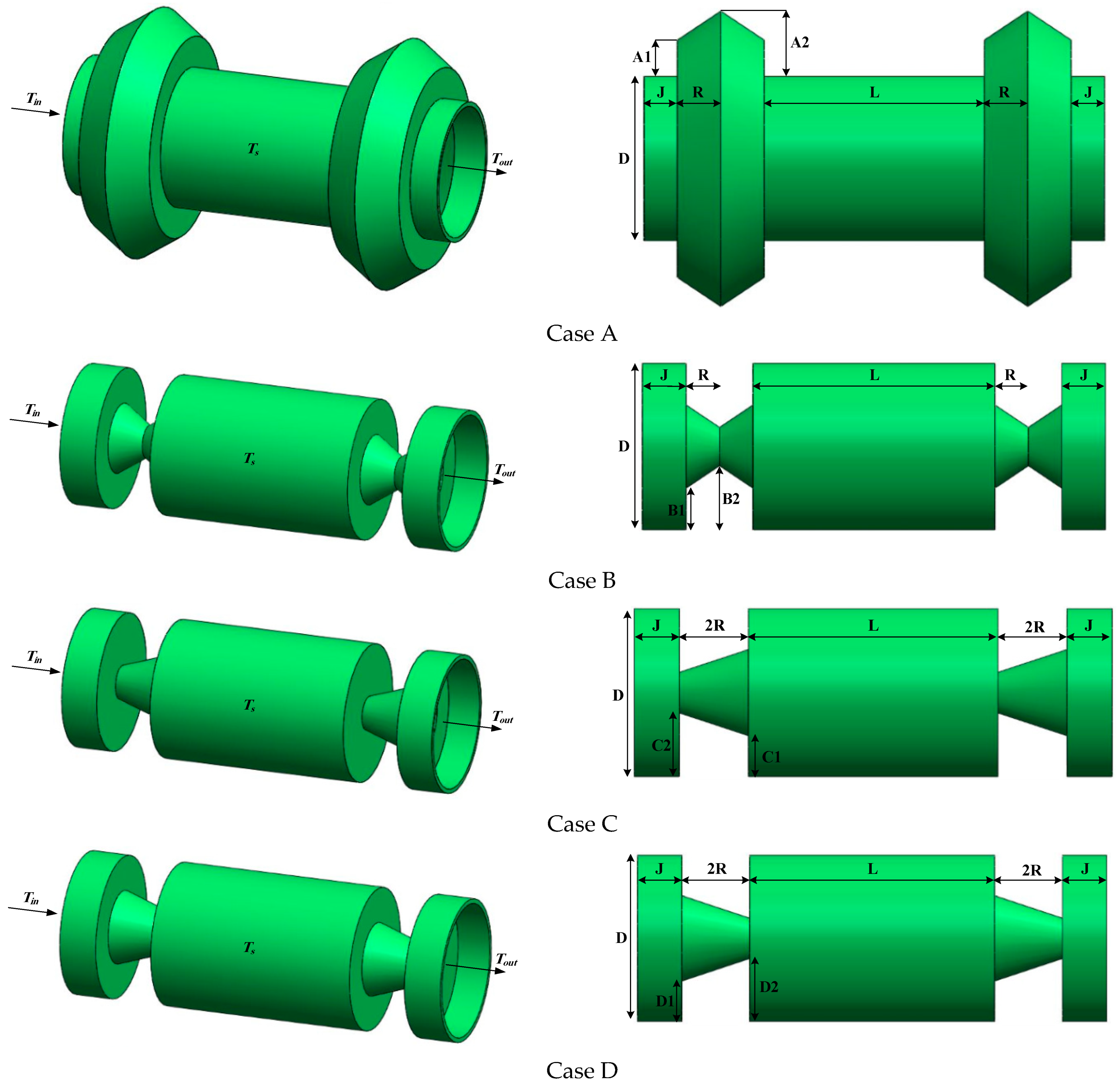
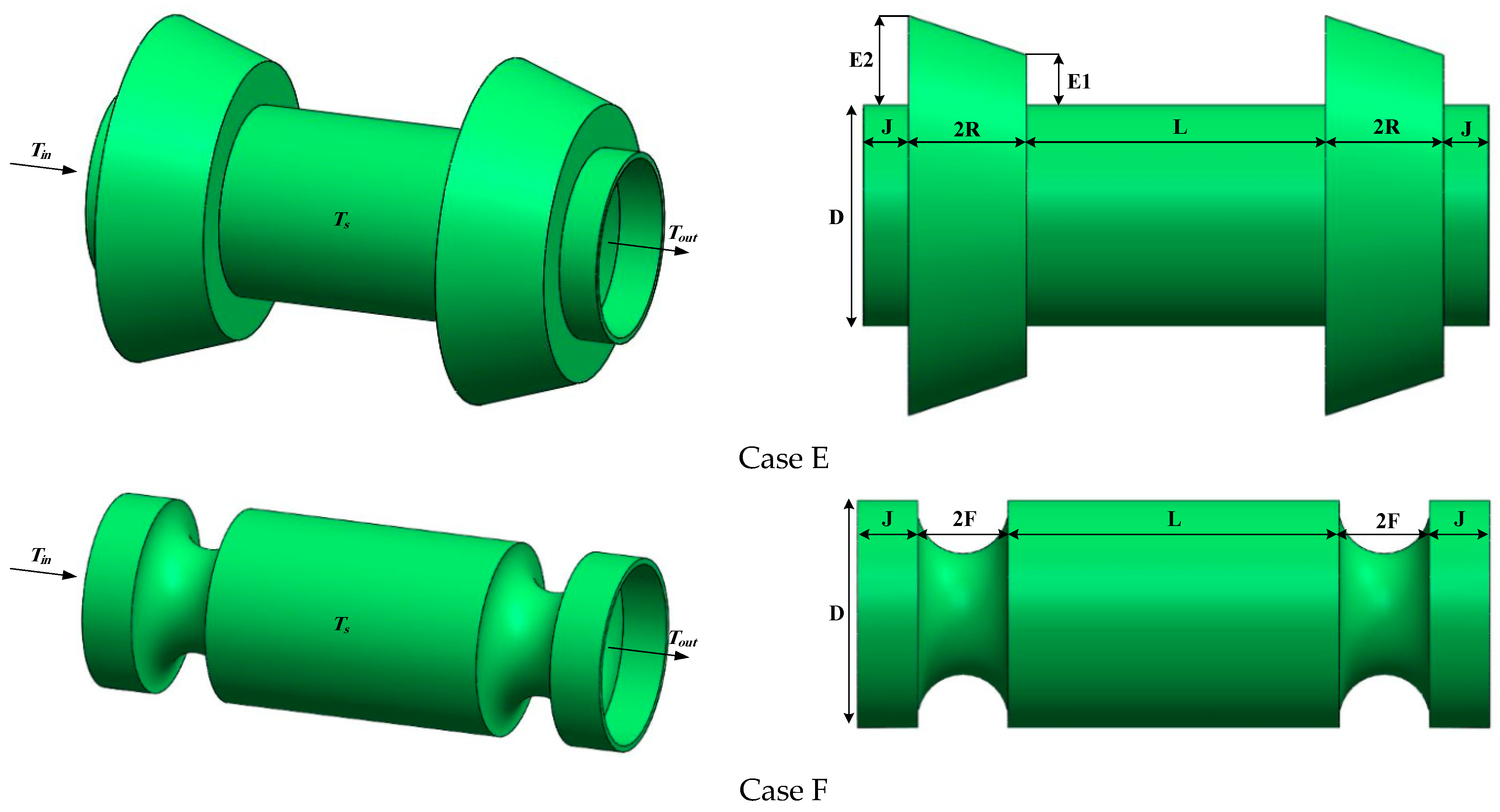
2.1. Physical Model
2.2. Governing Equations
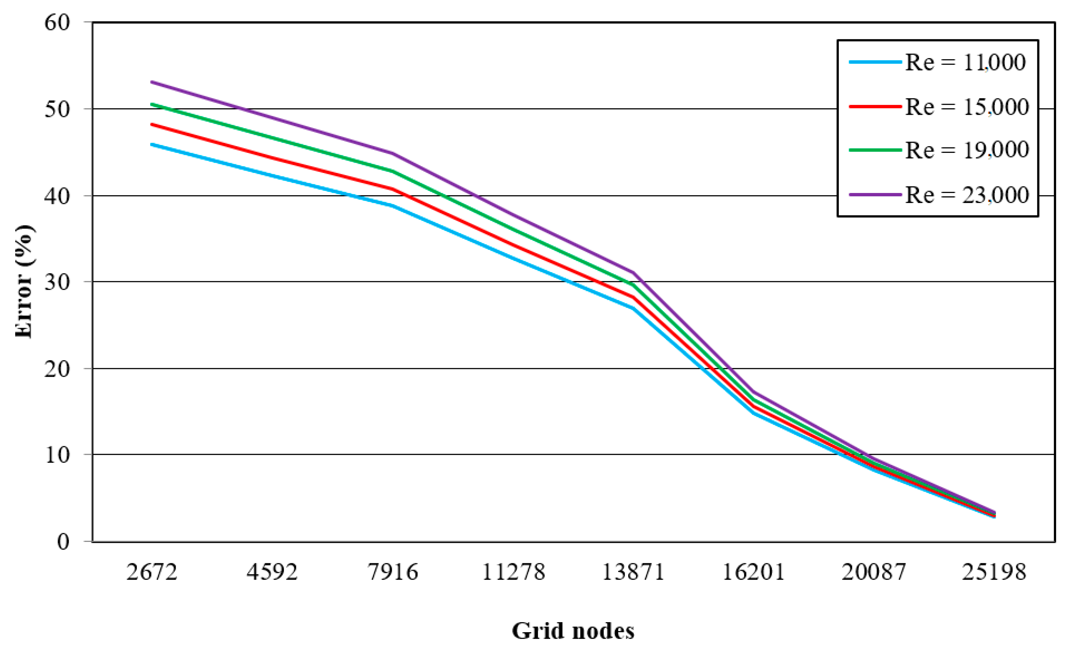
2.3. Grid Mesh Independence Test
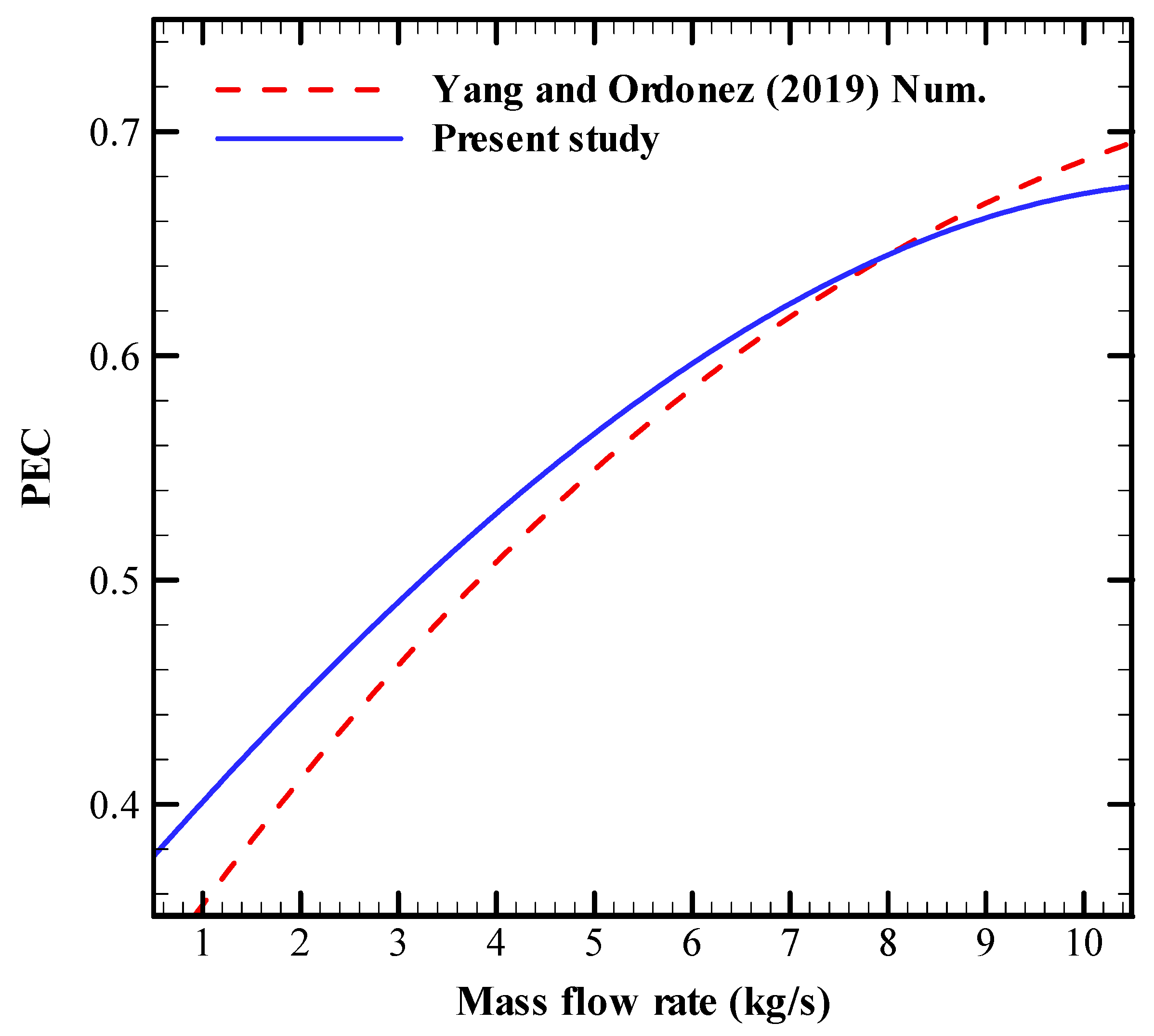
2.4. Validation
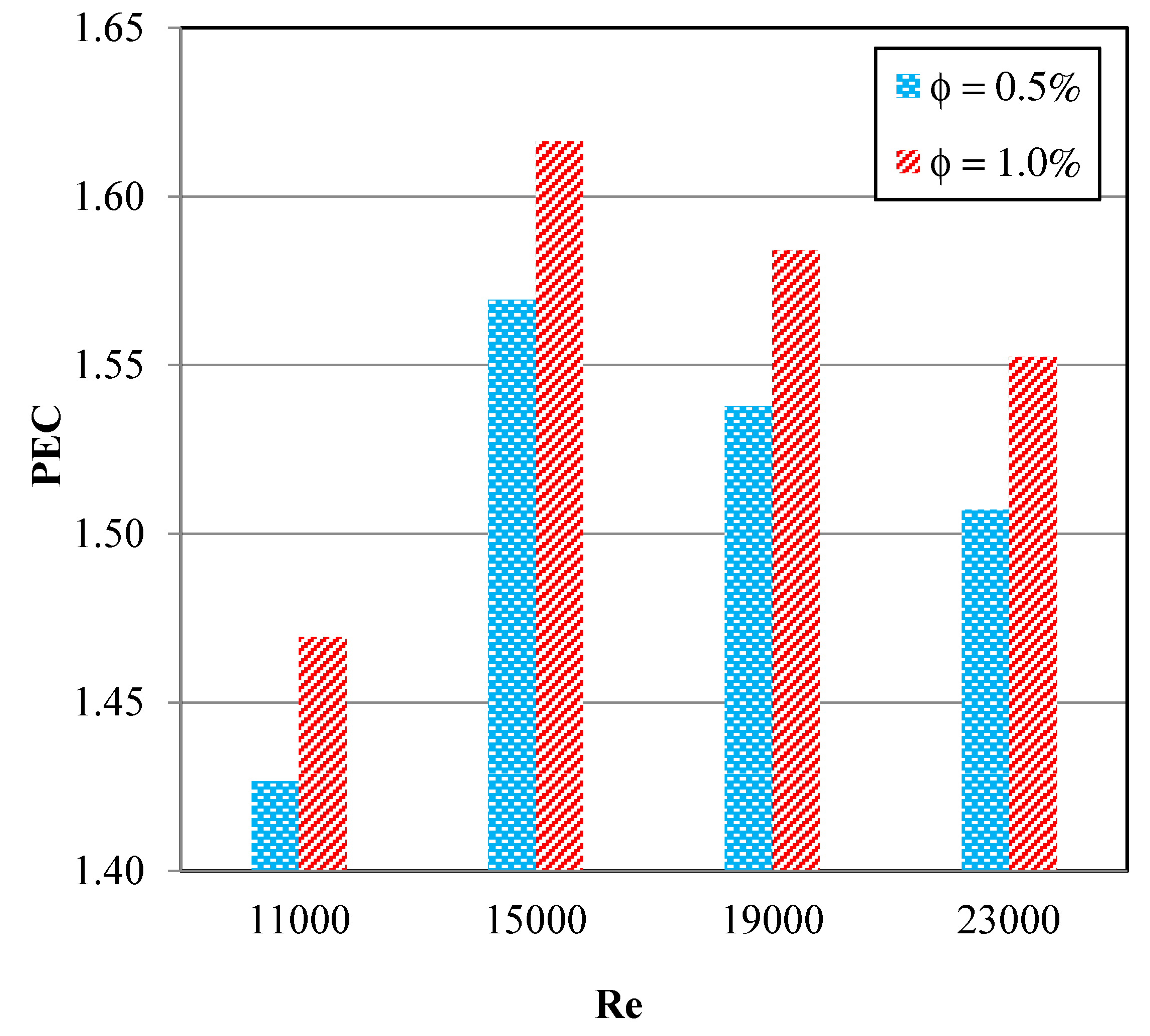
3. Results and Discussion
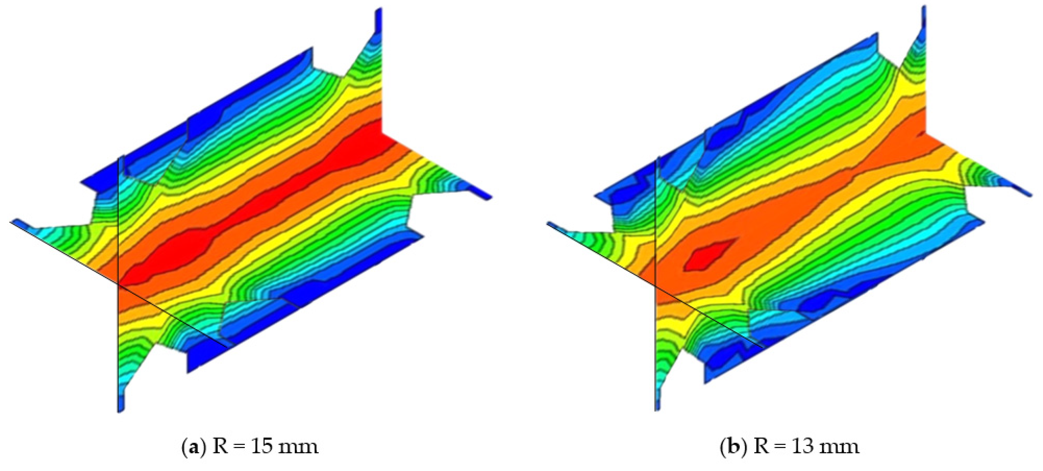
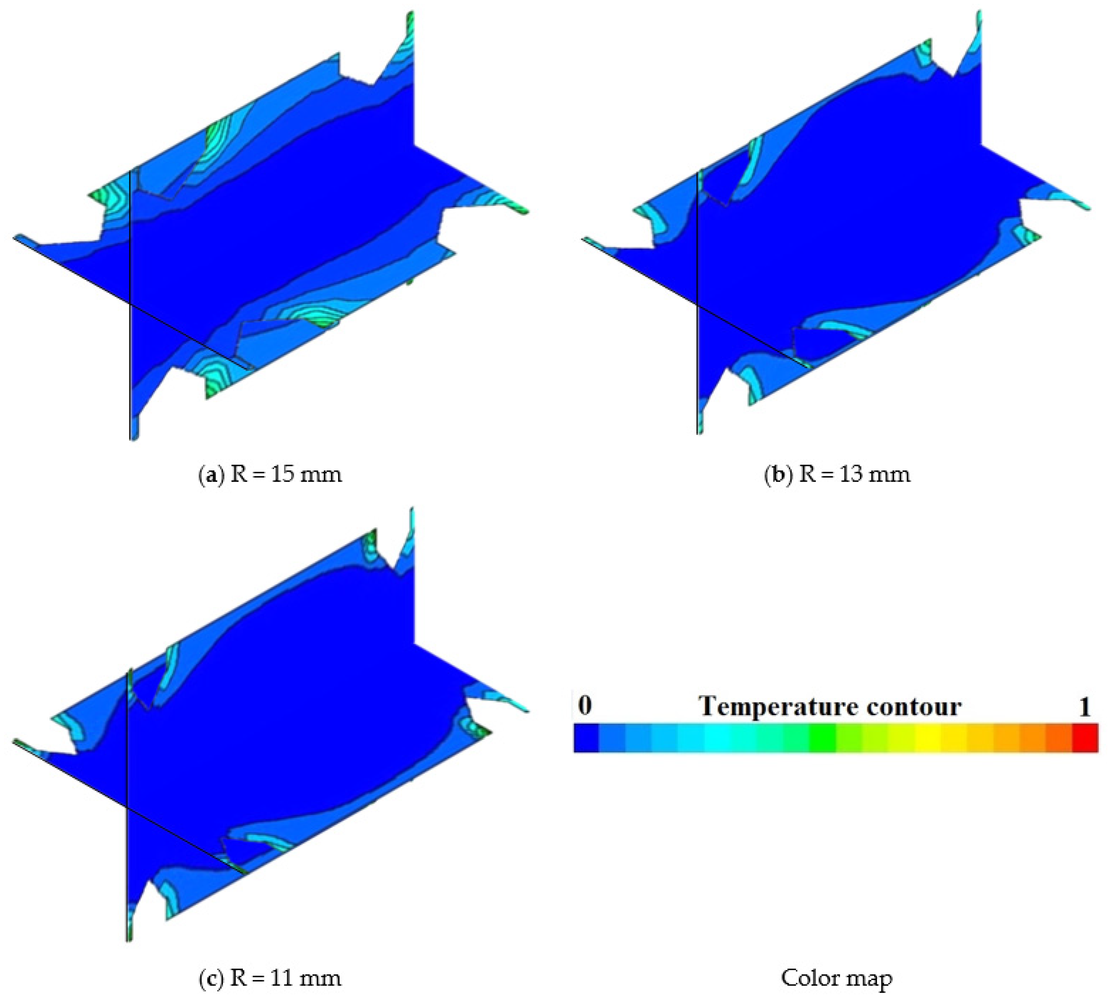
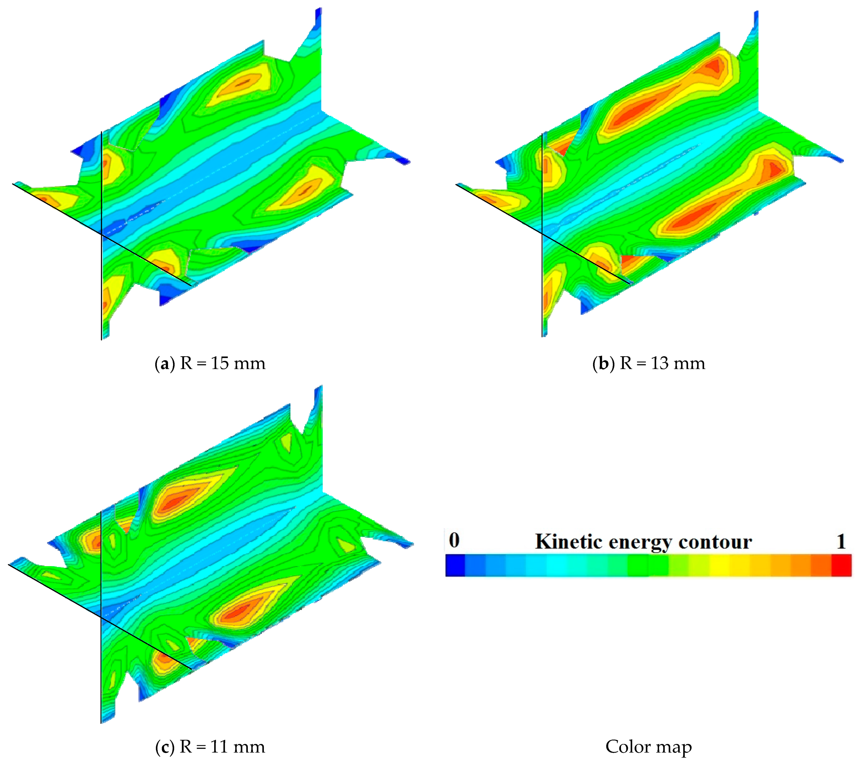
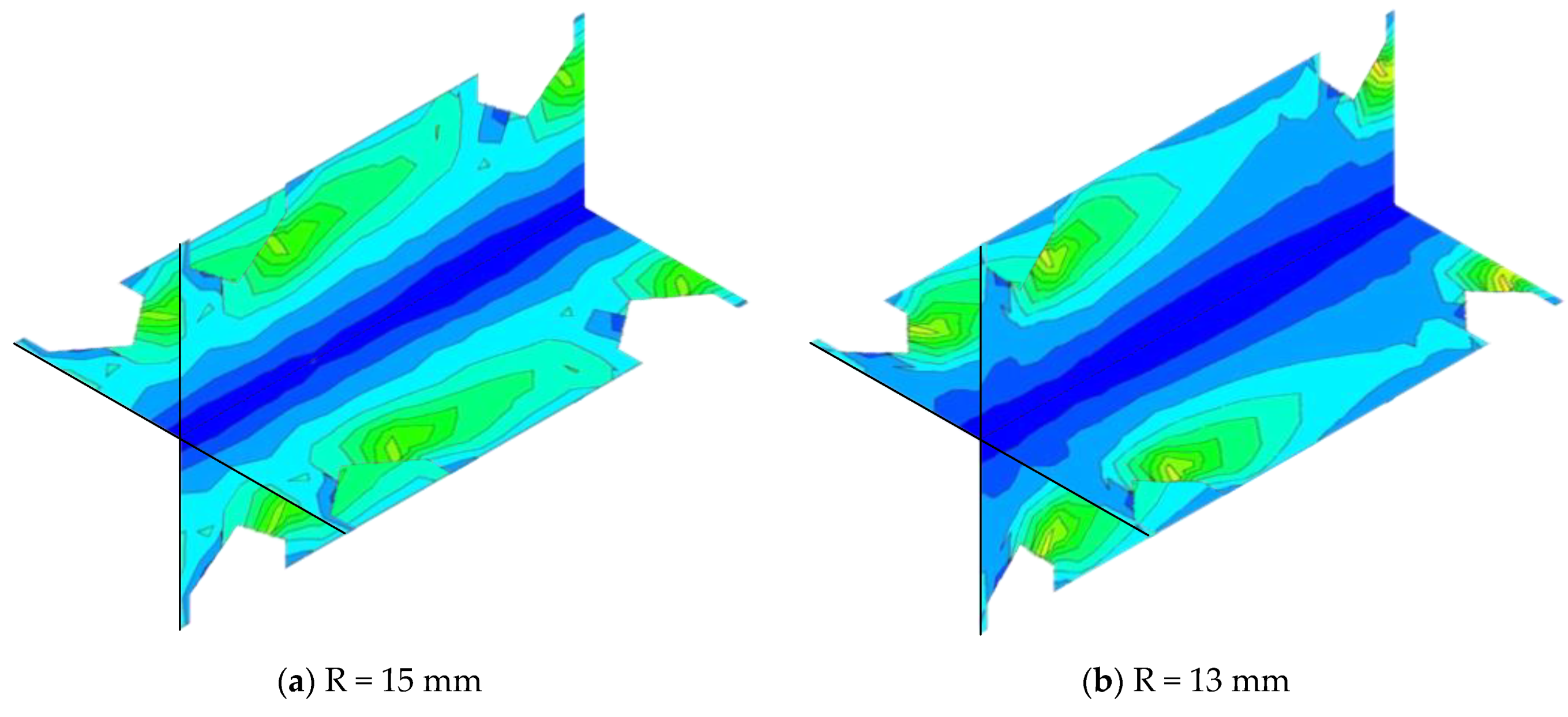
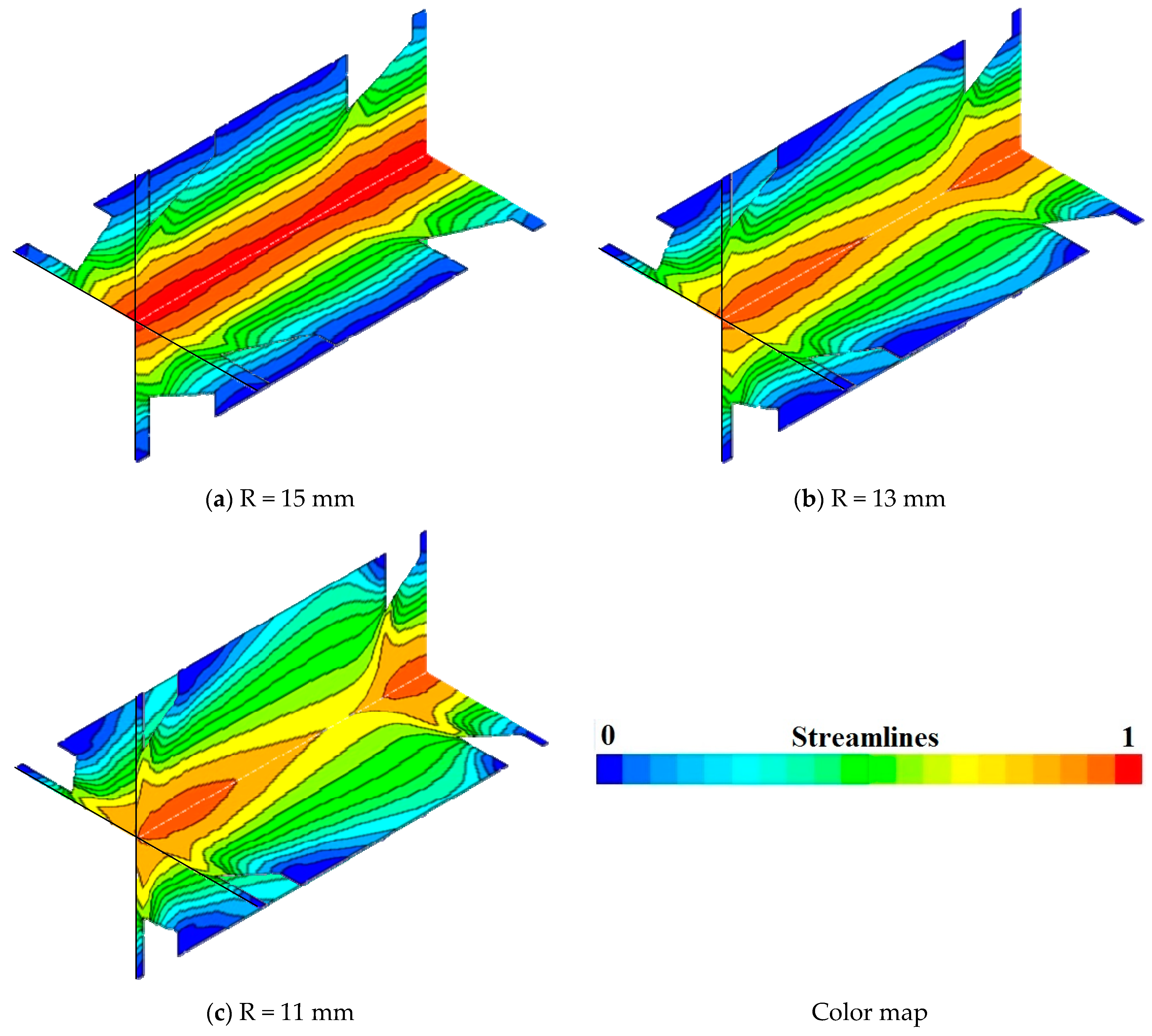
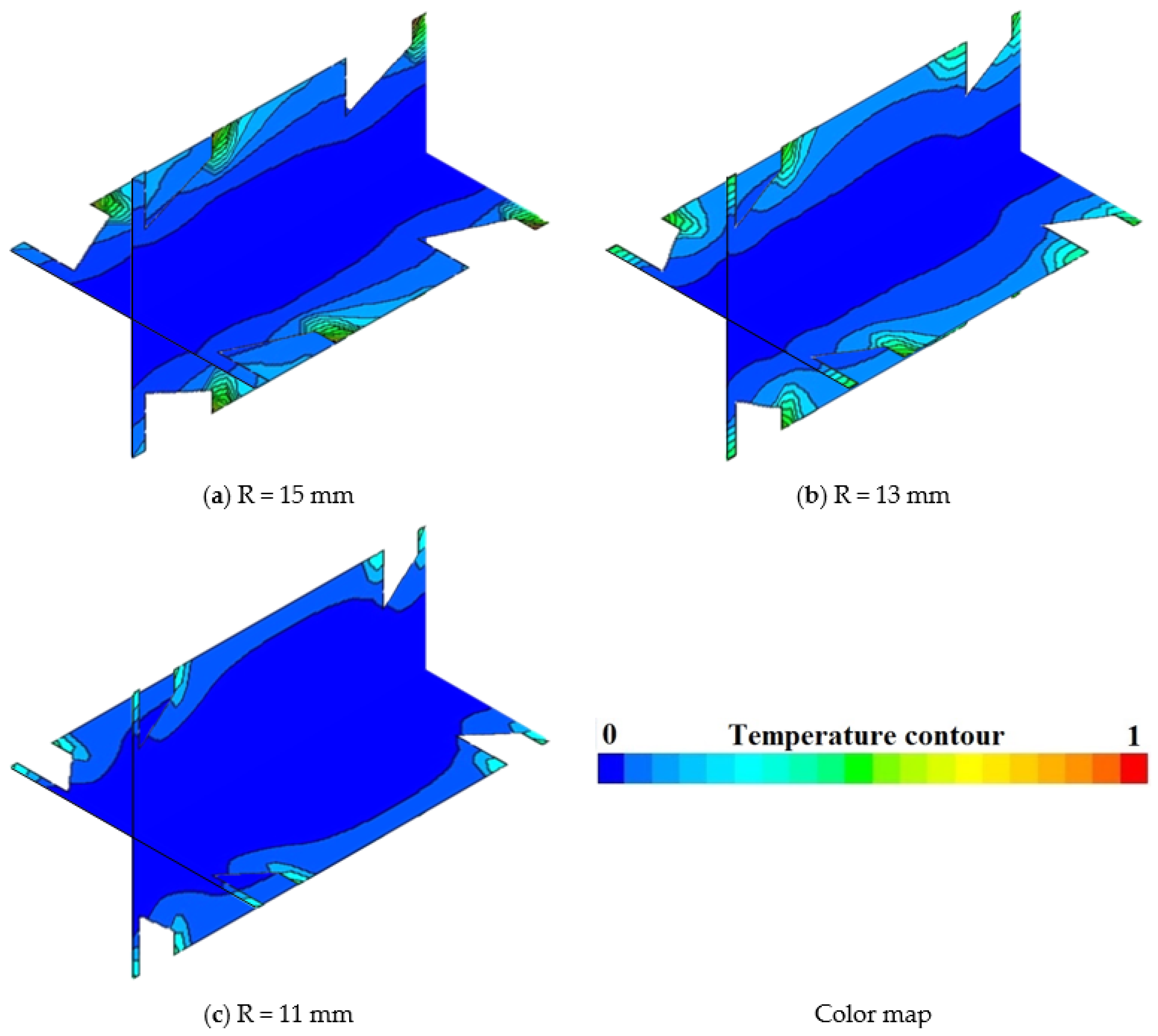
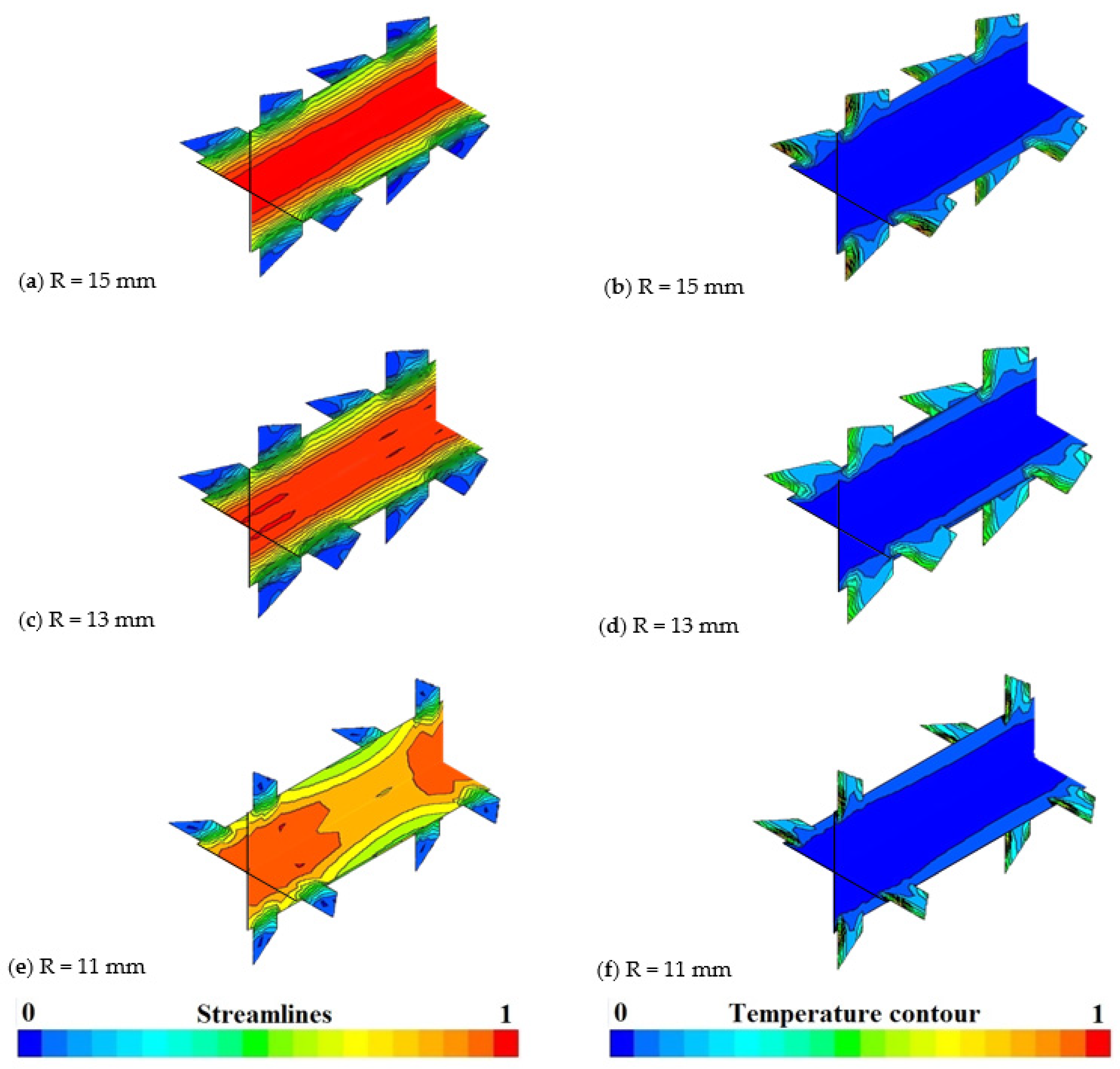
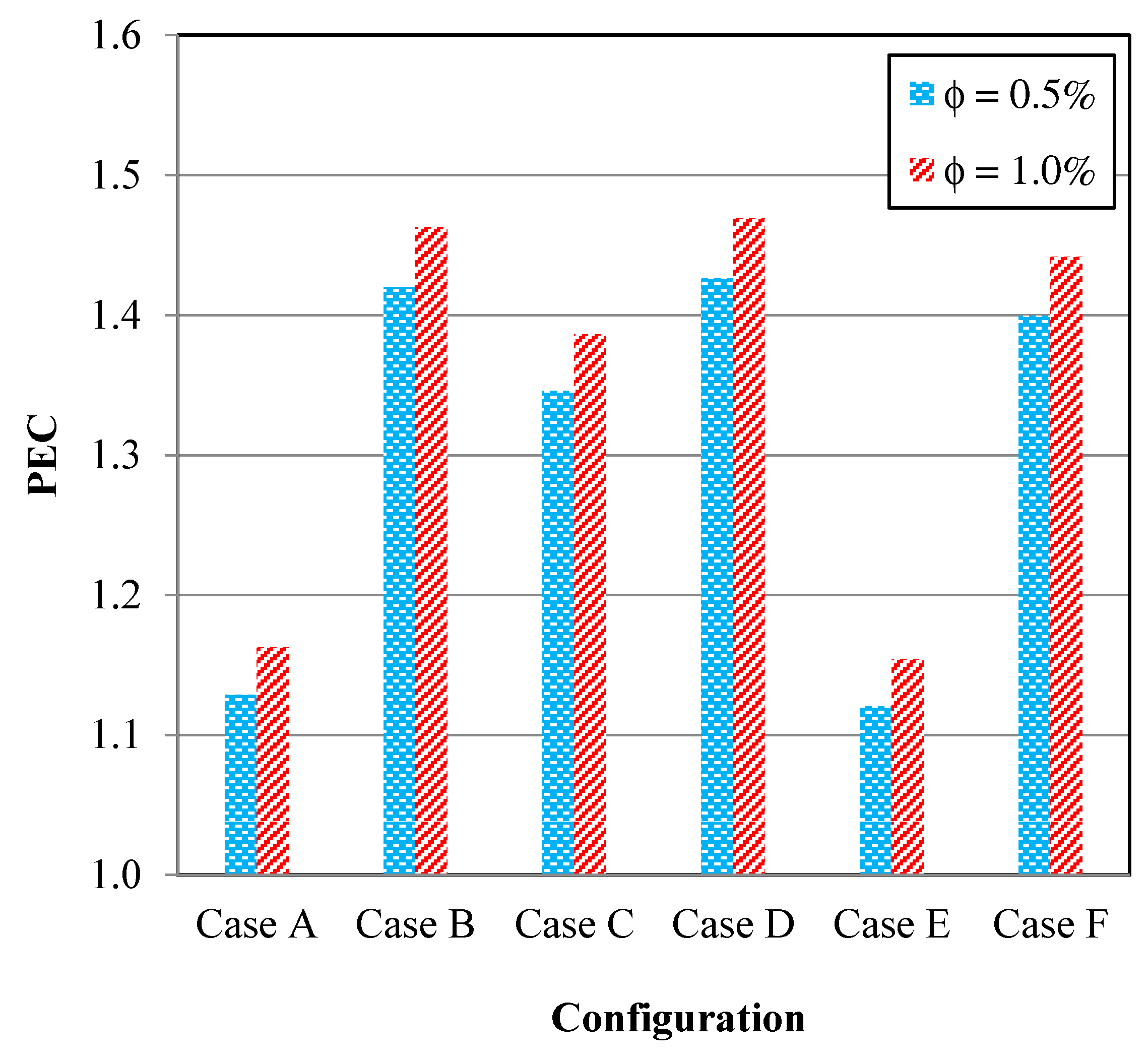
3.1. Case A
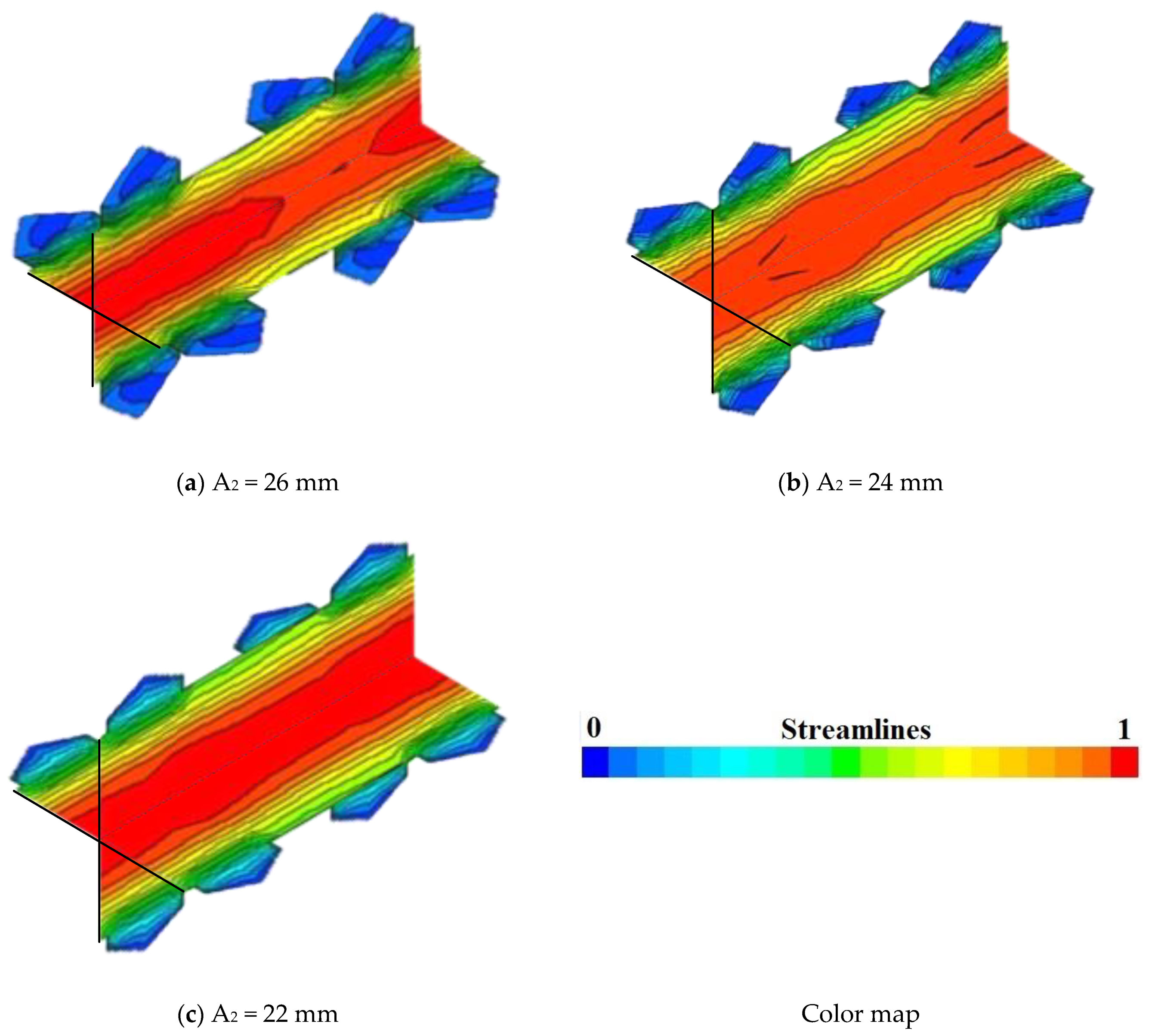
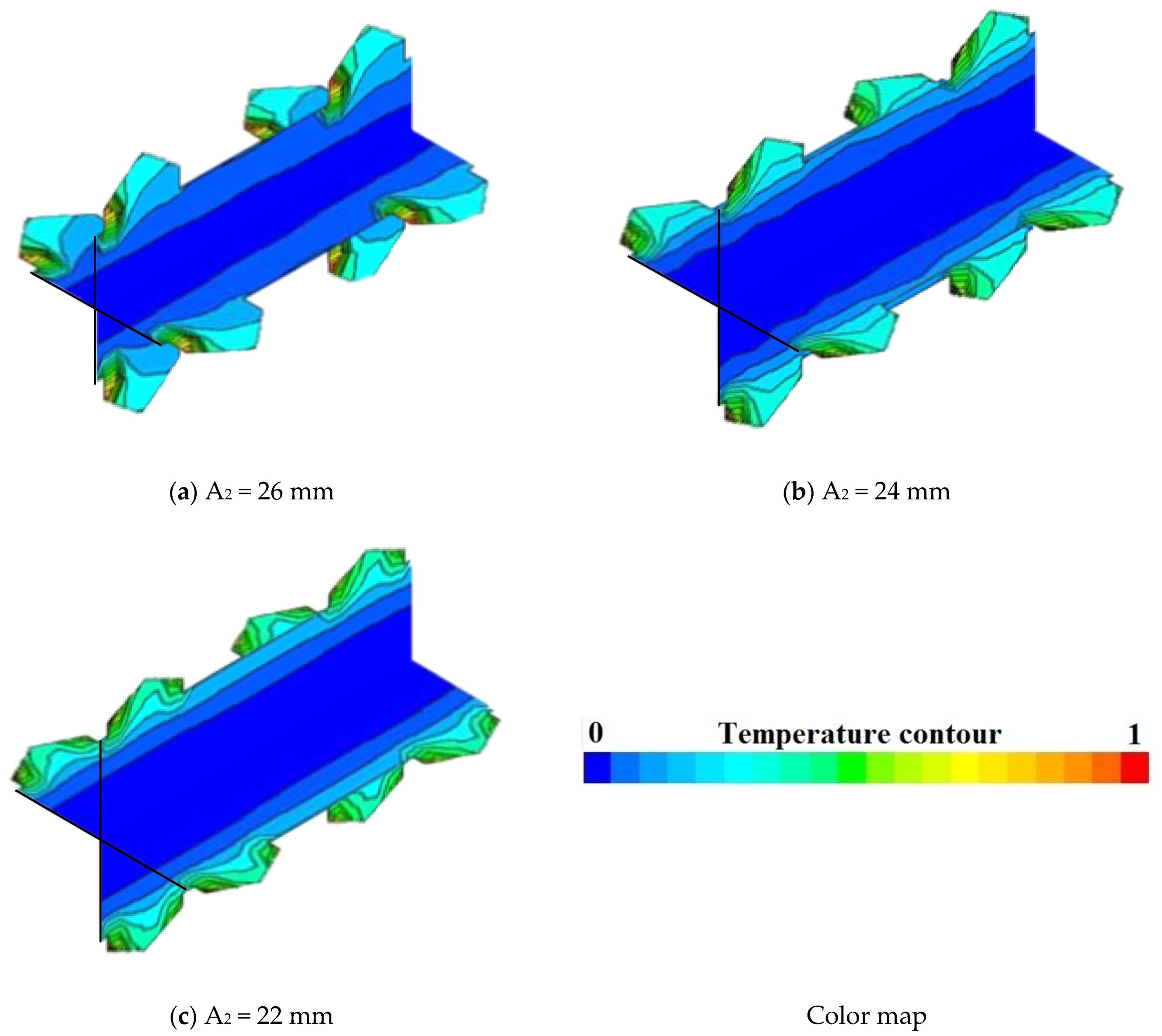
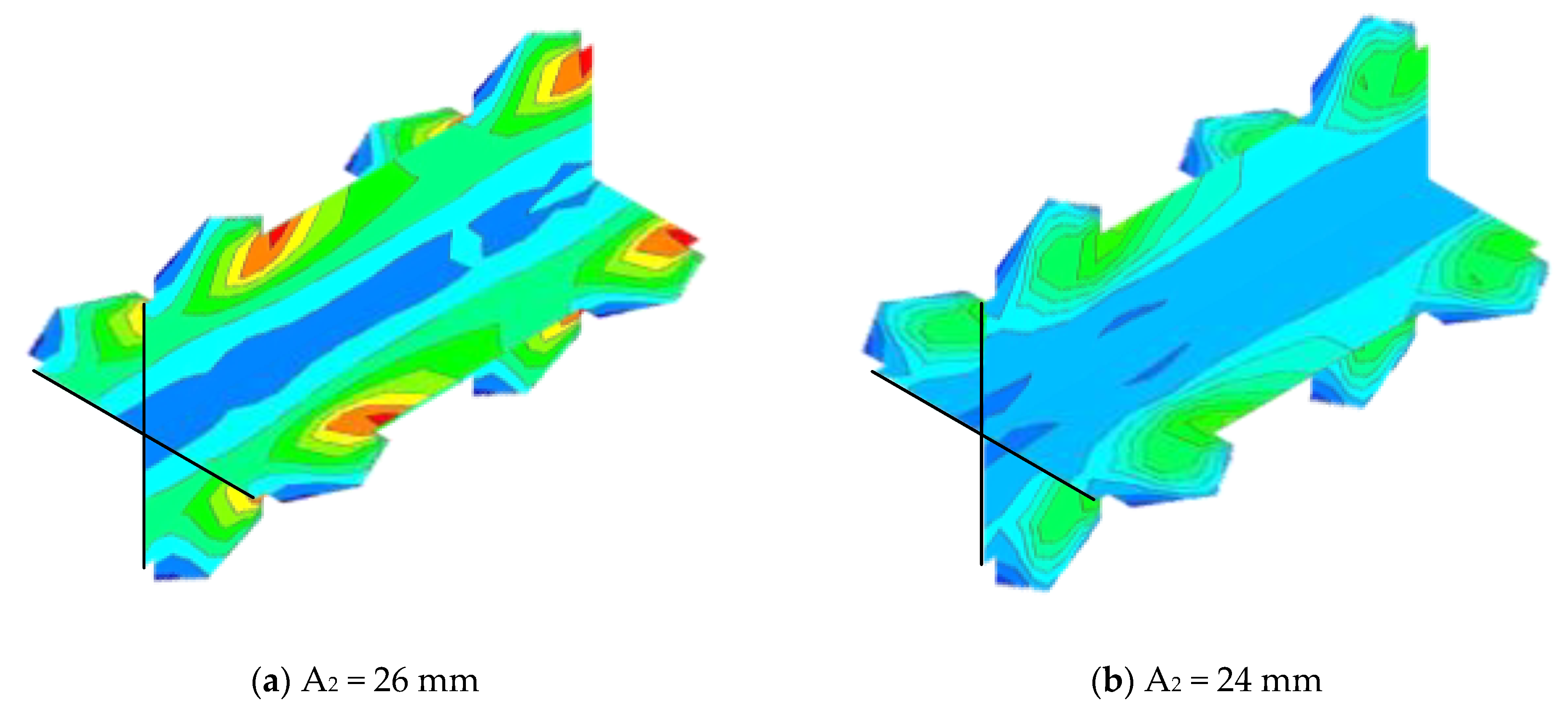
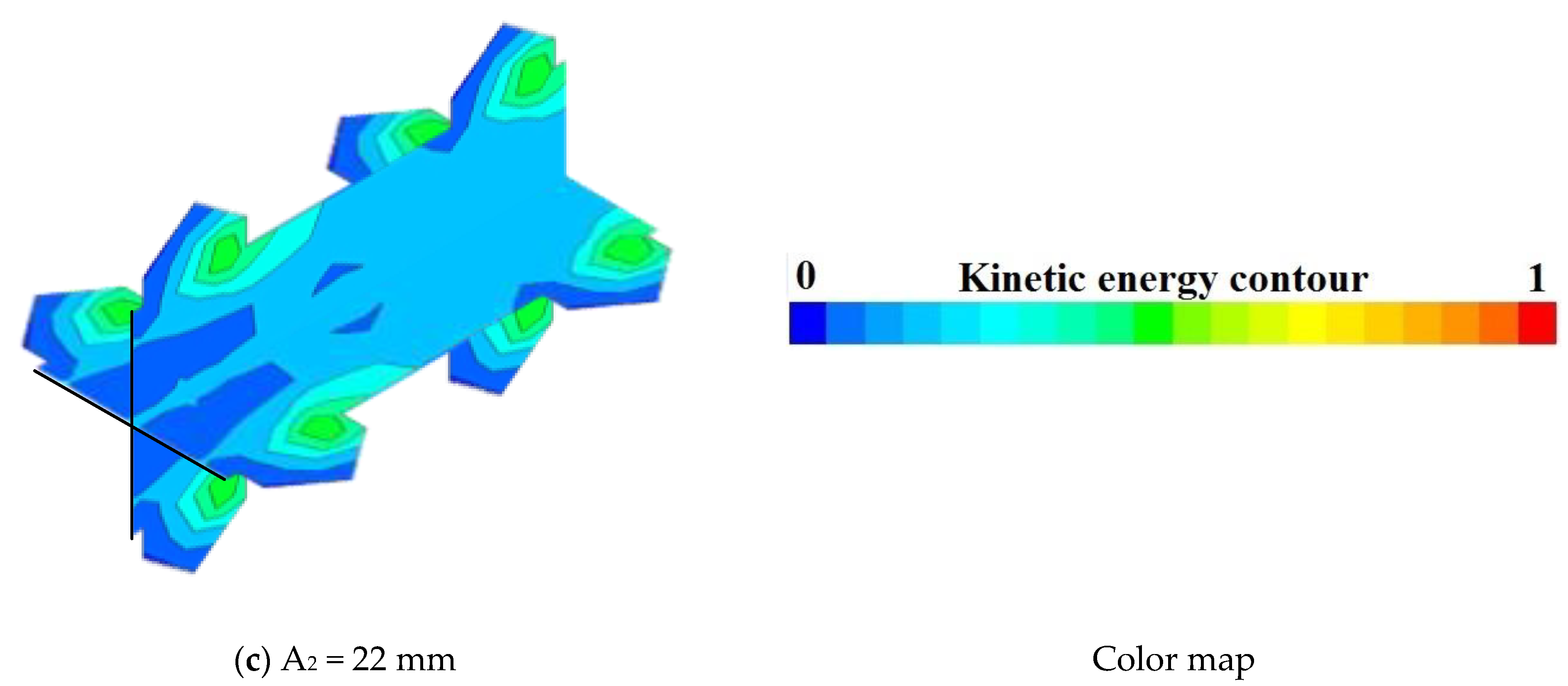
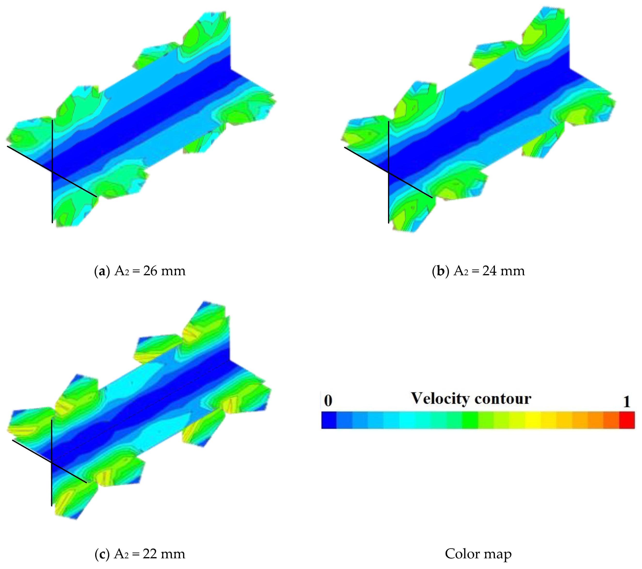
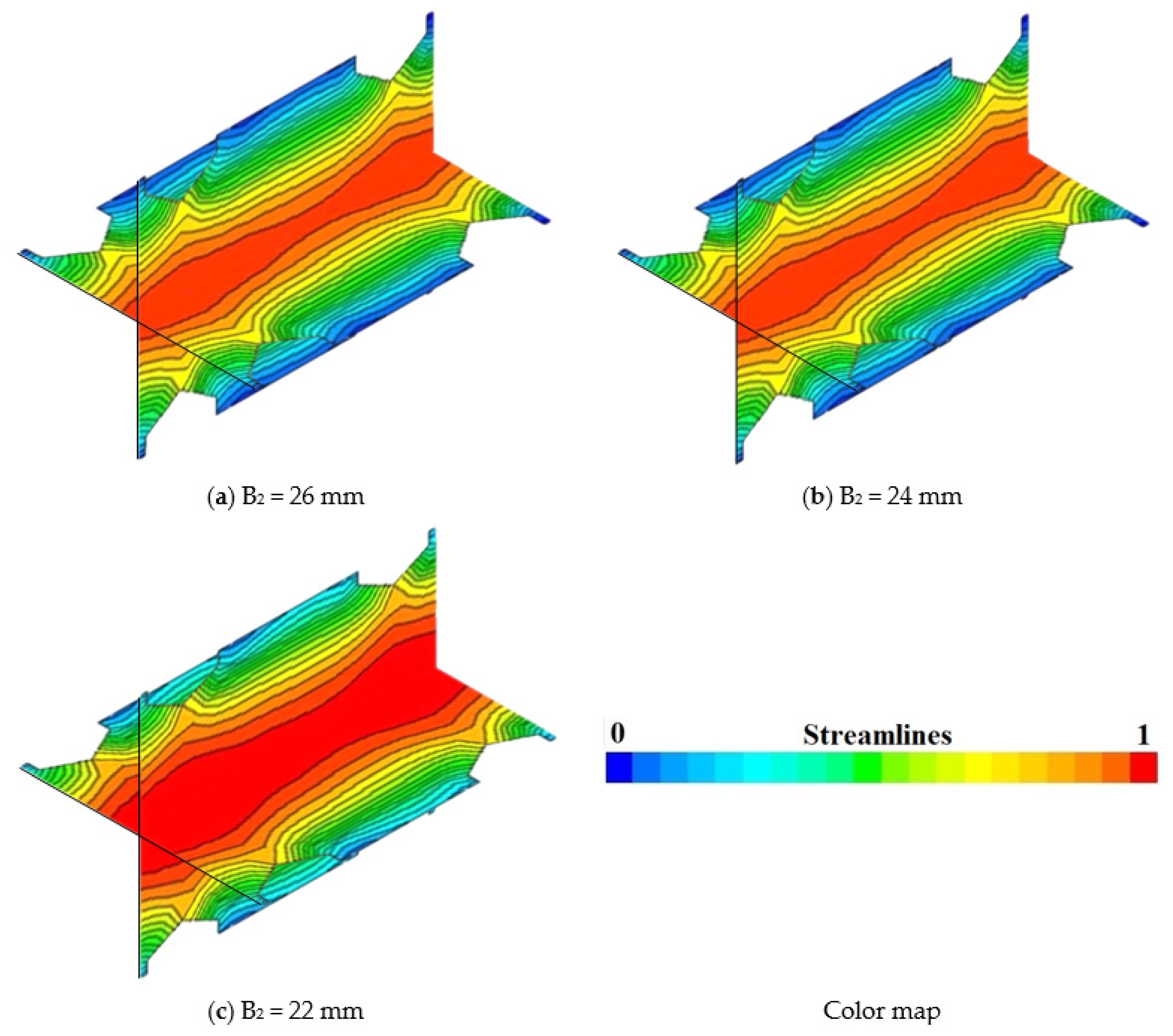
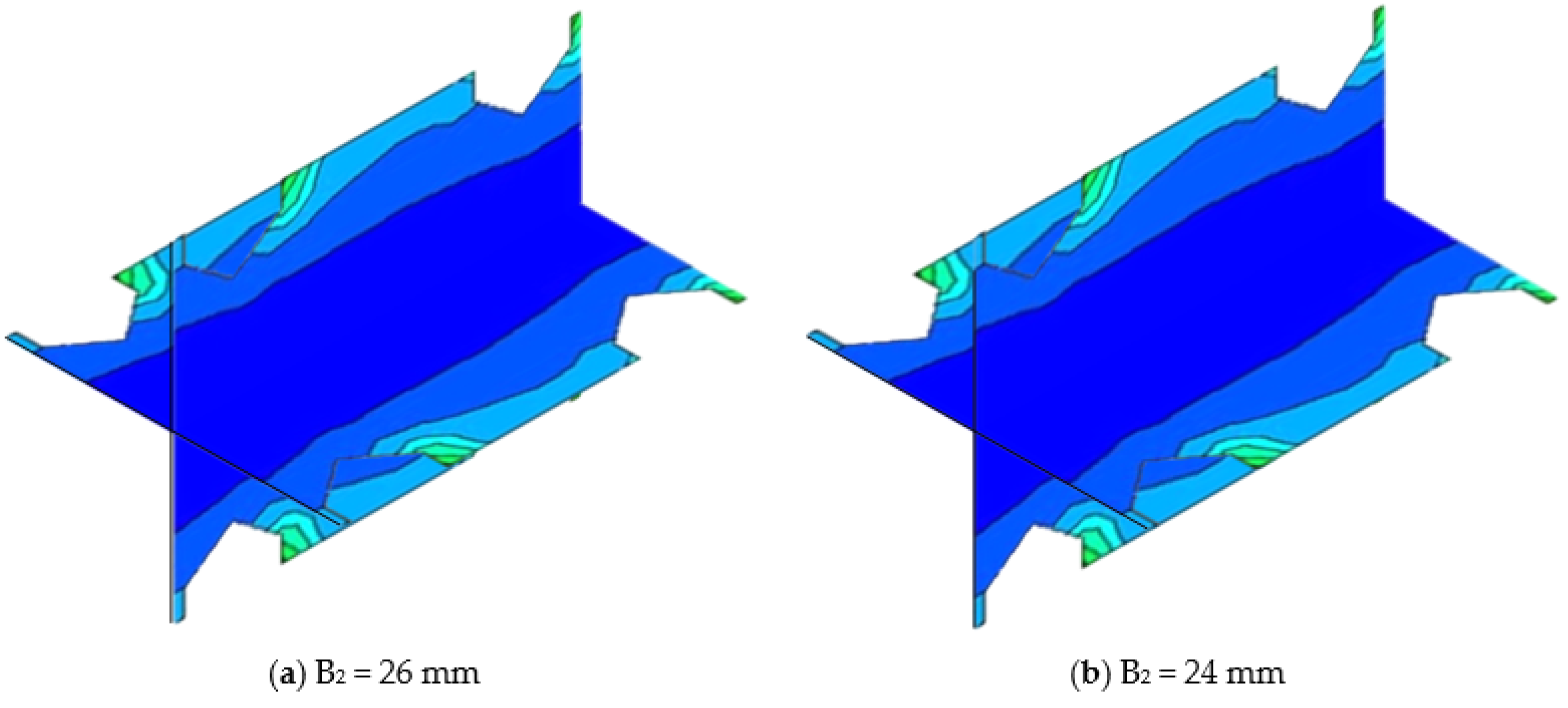
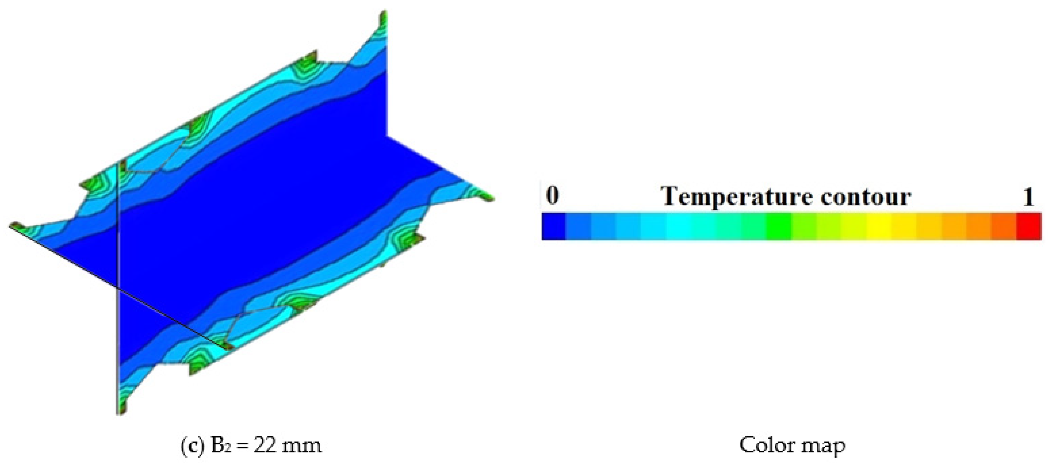
3.2. Case B
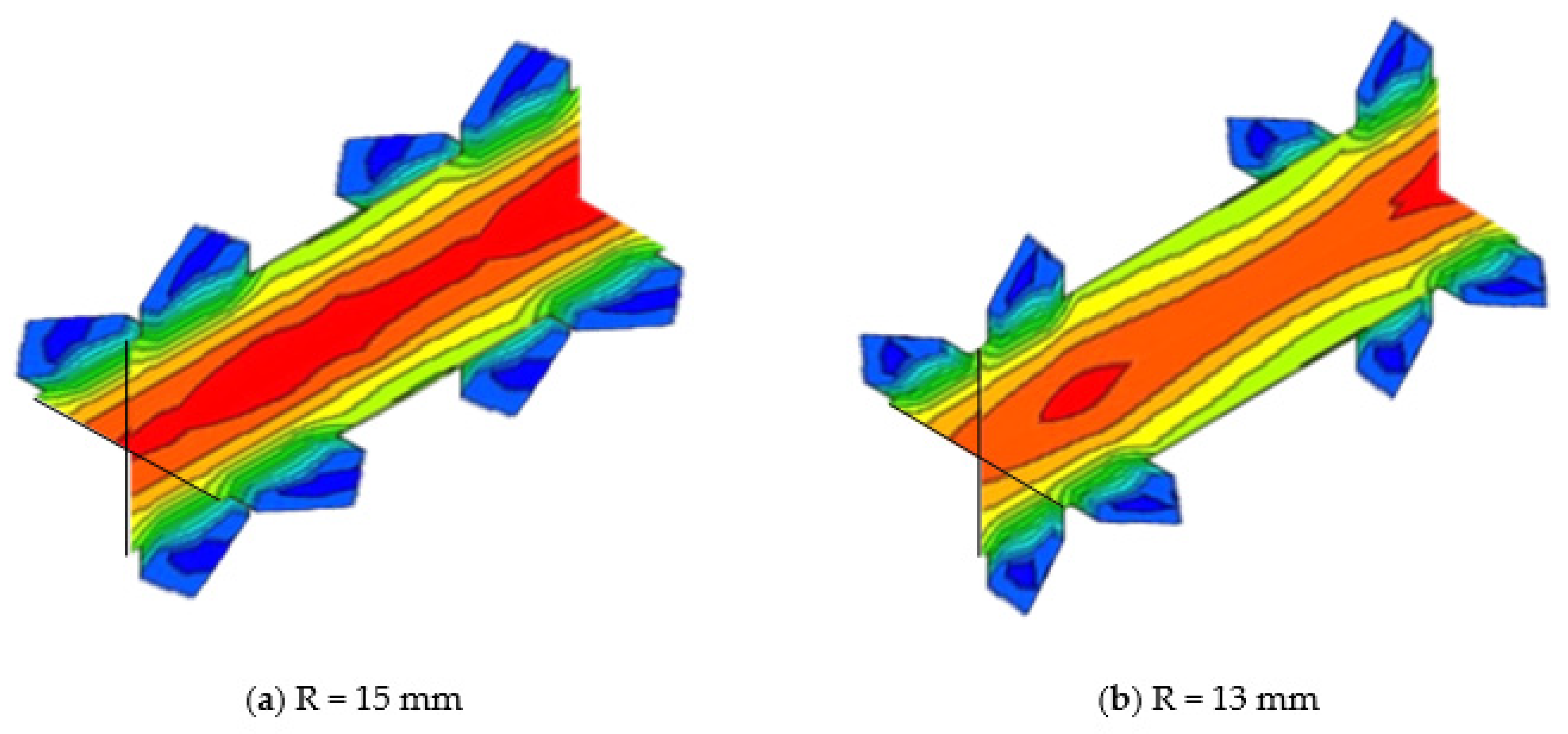
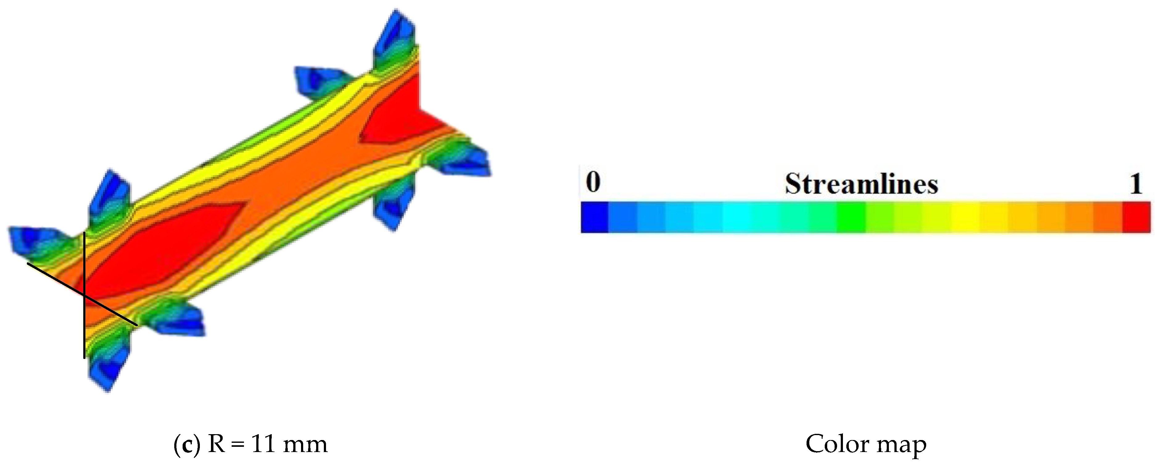
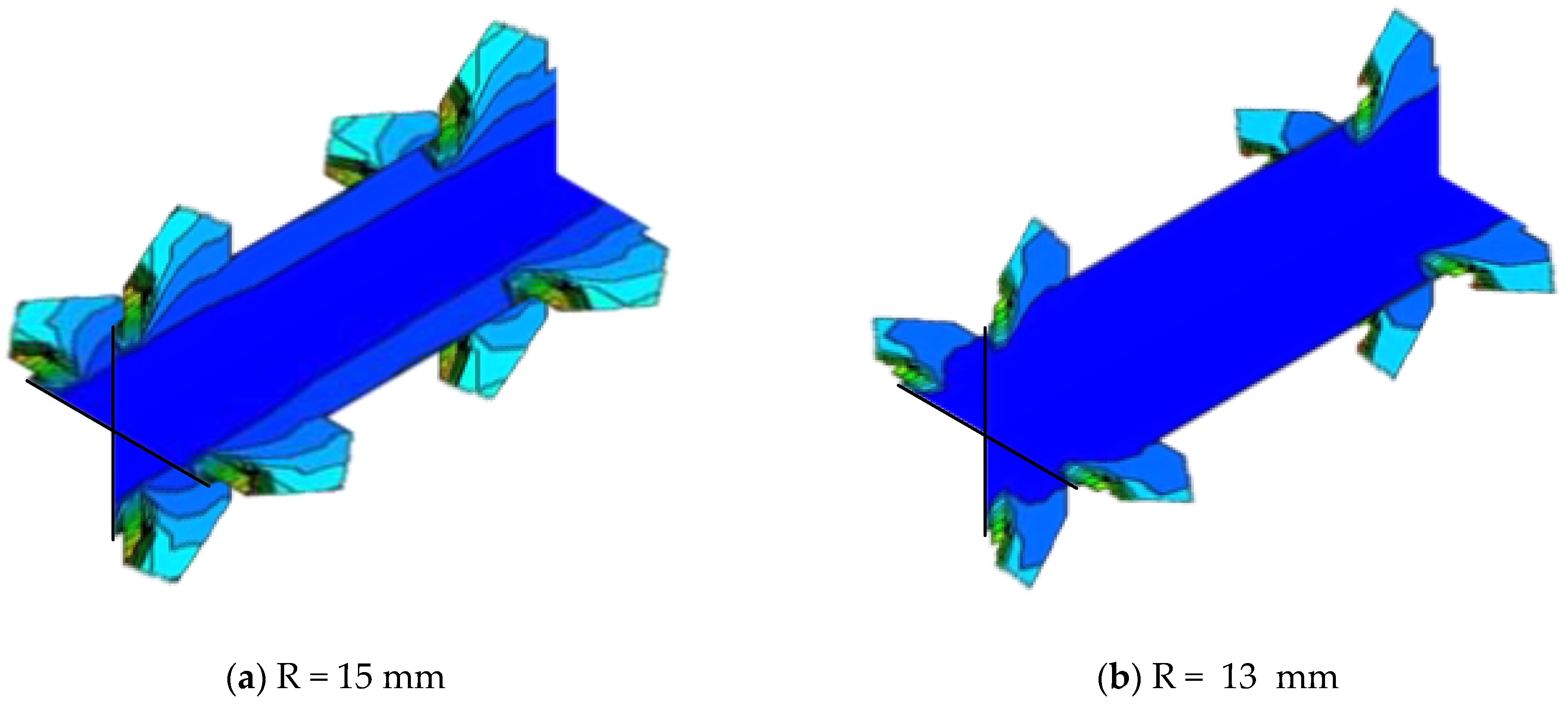
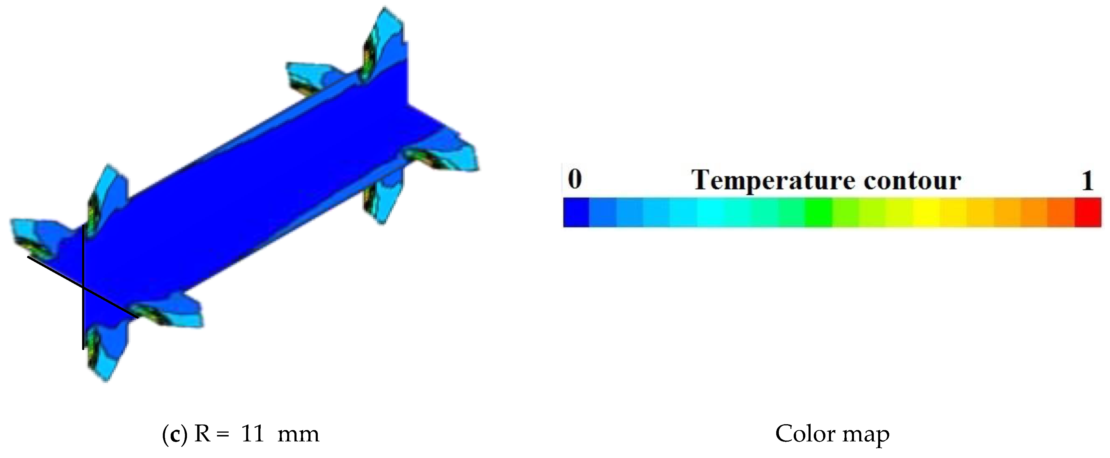
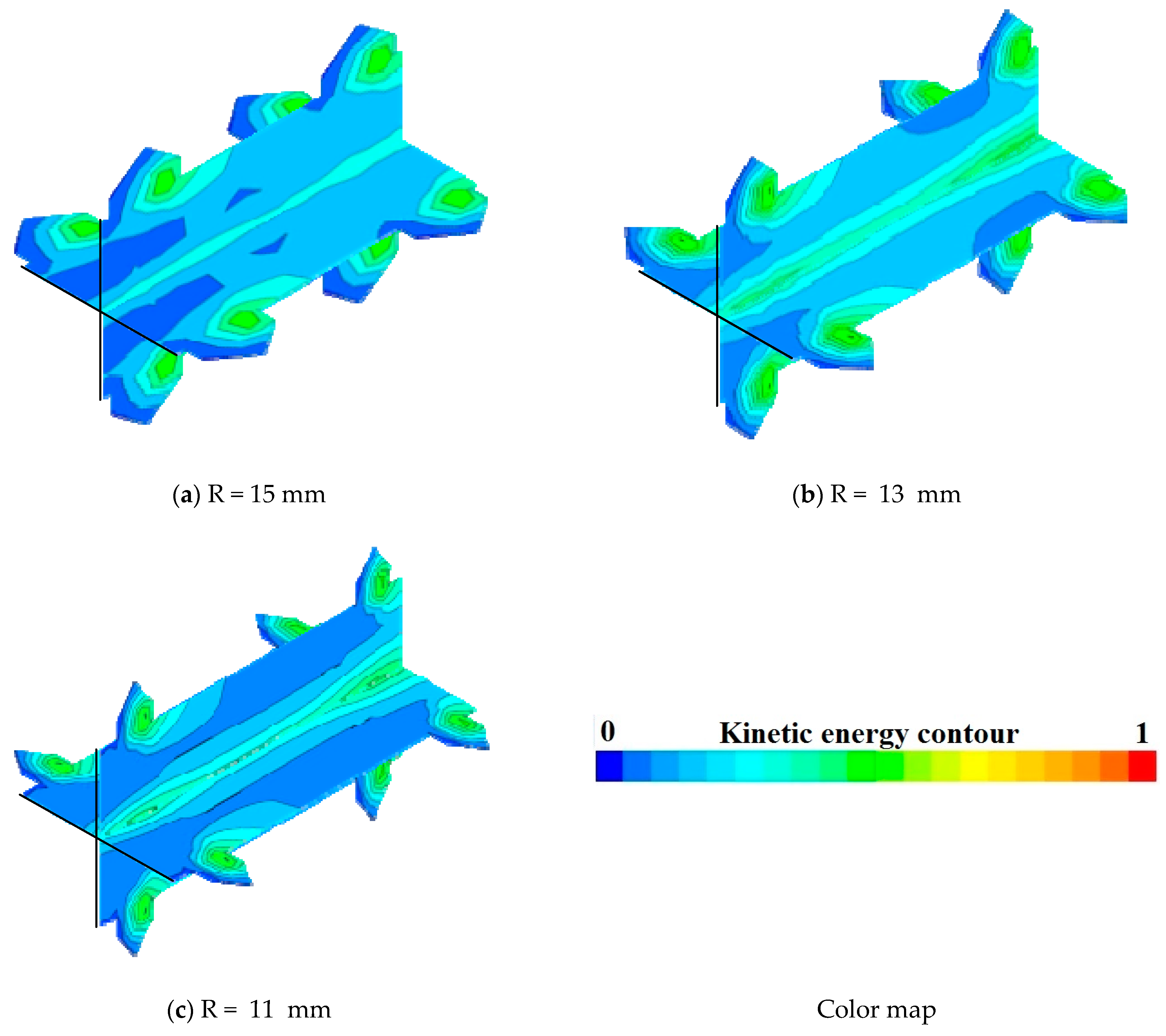
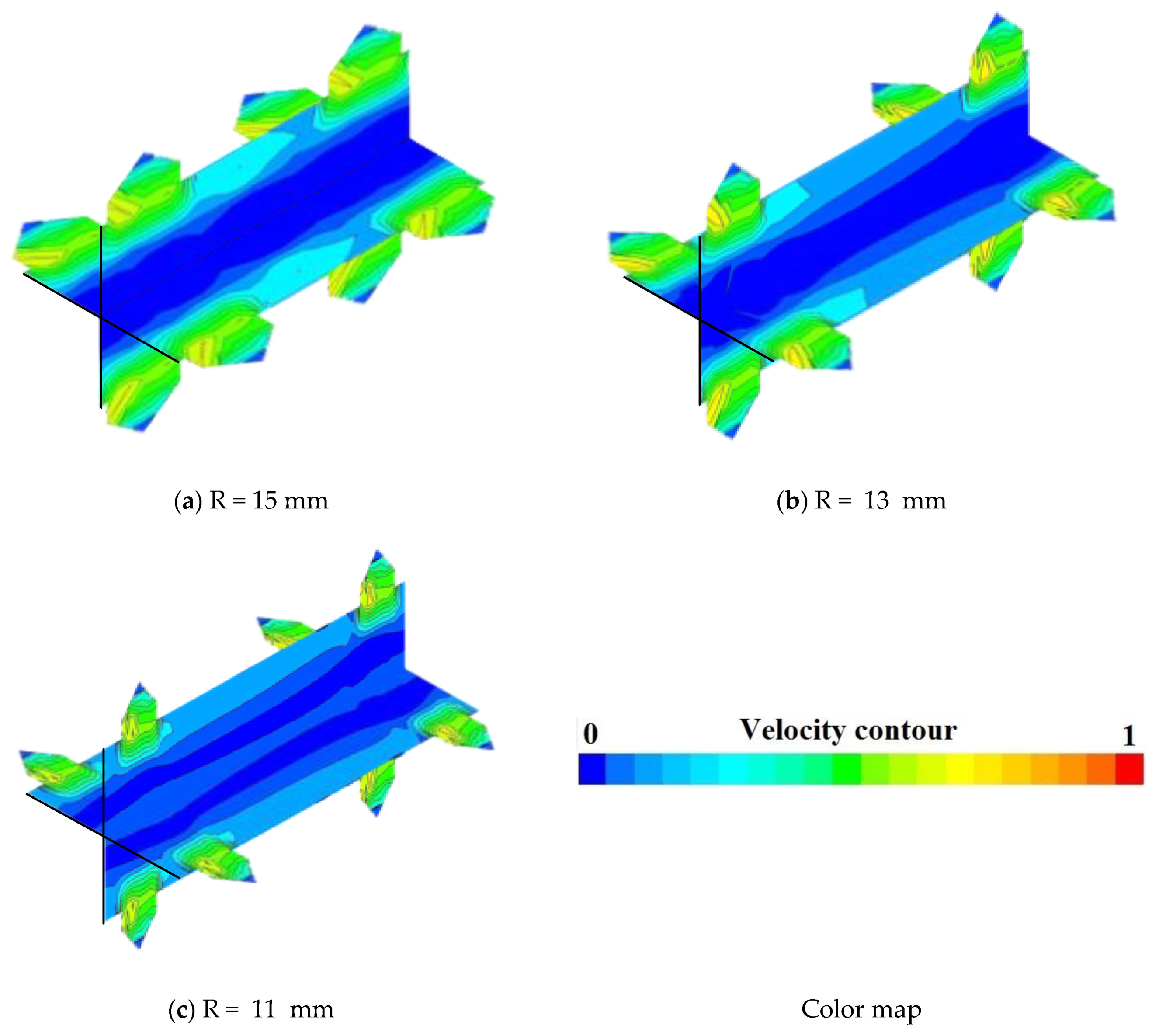
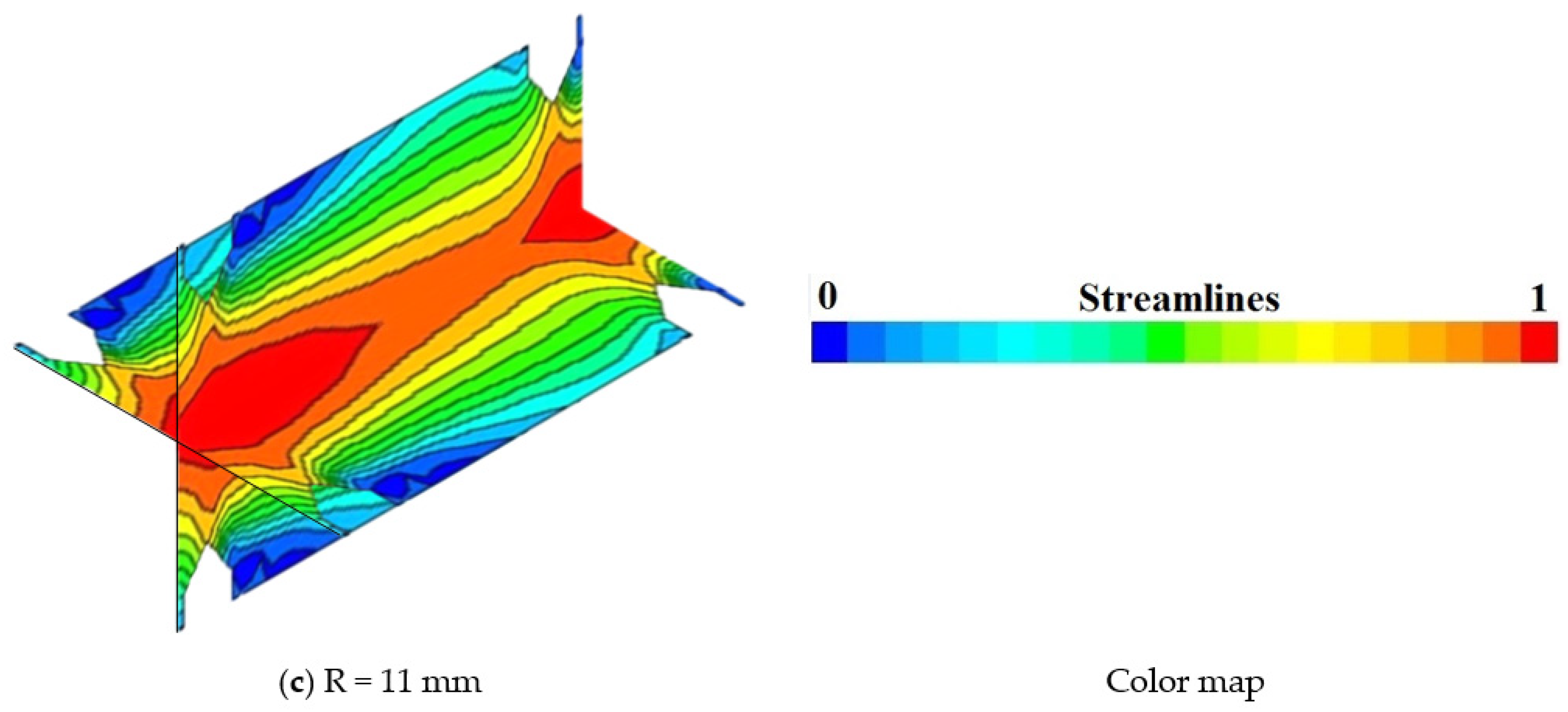
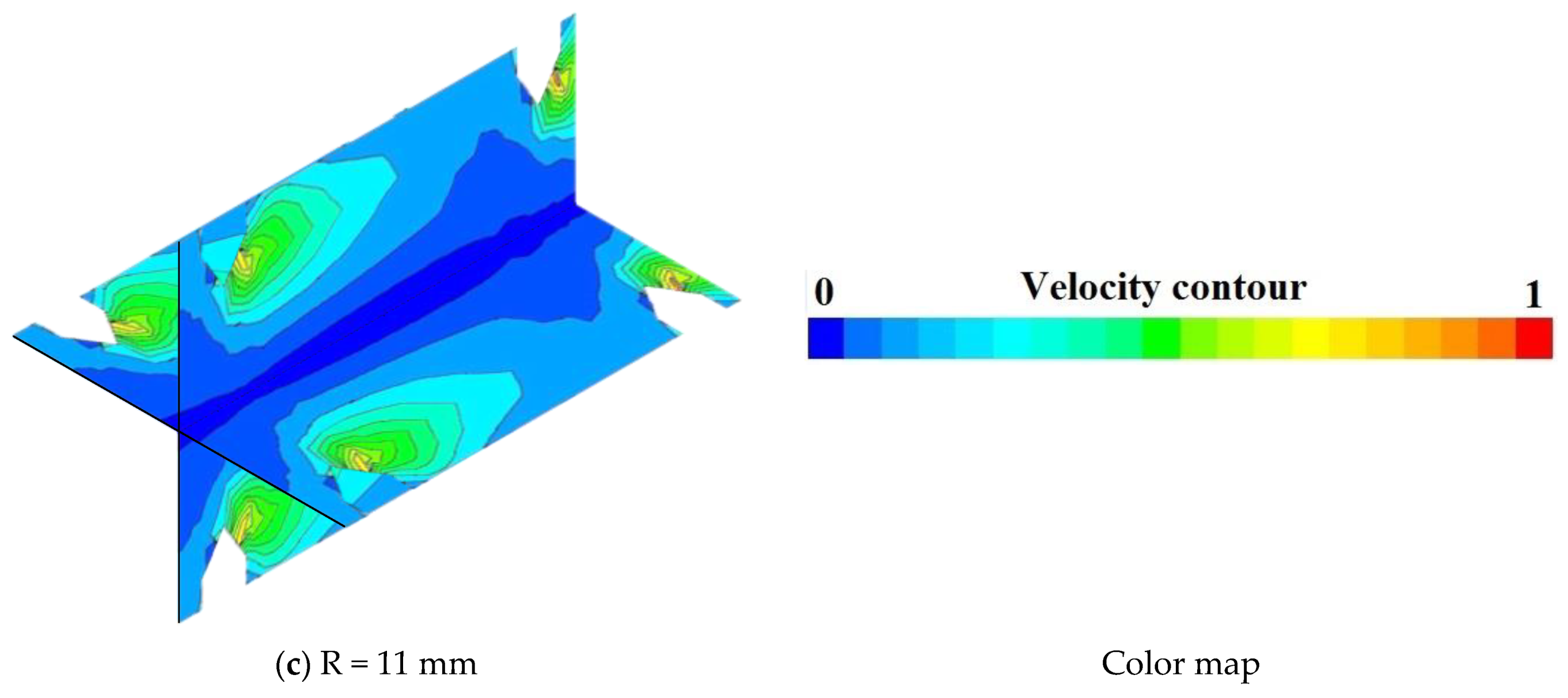
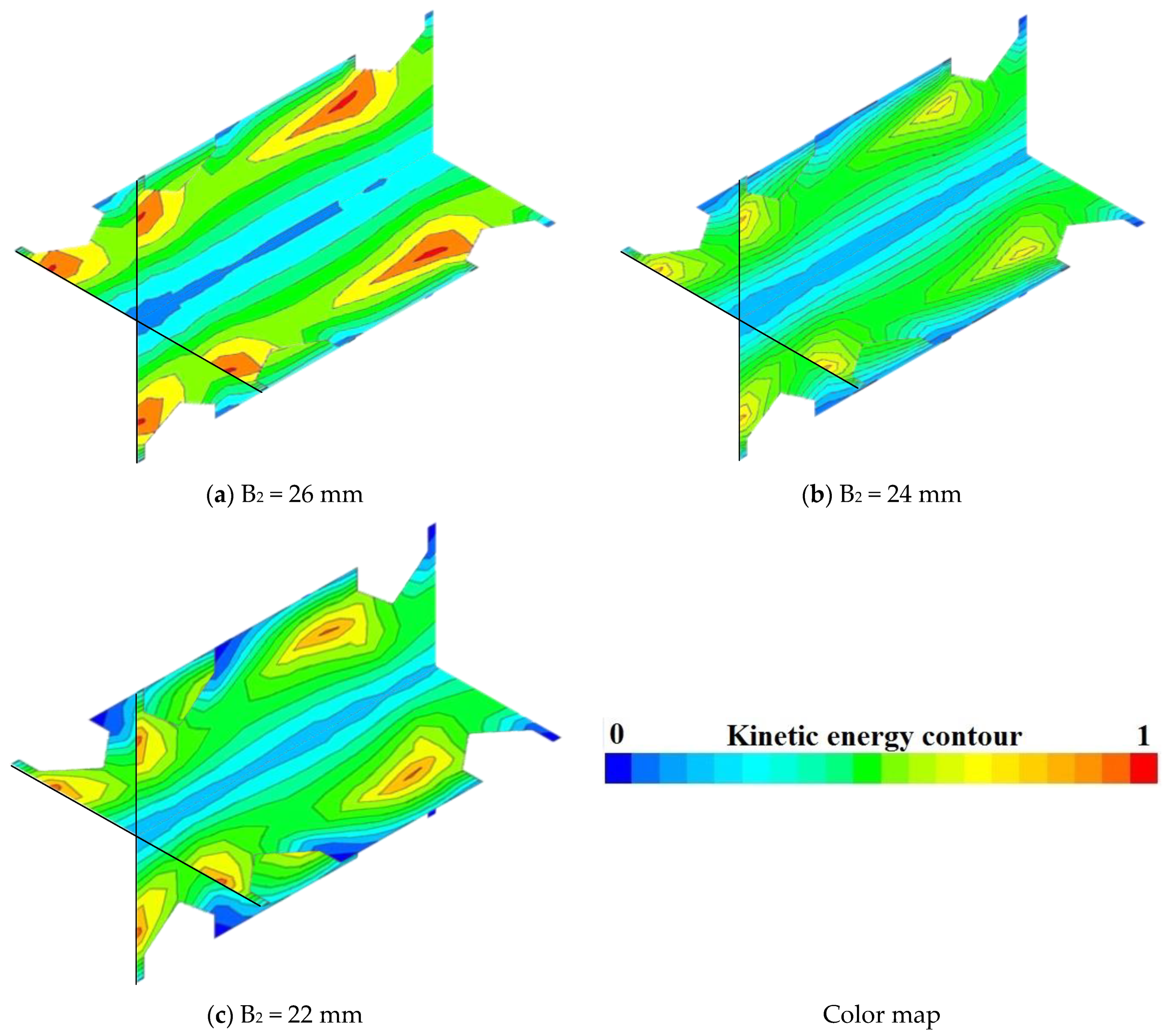
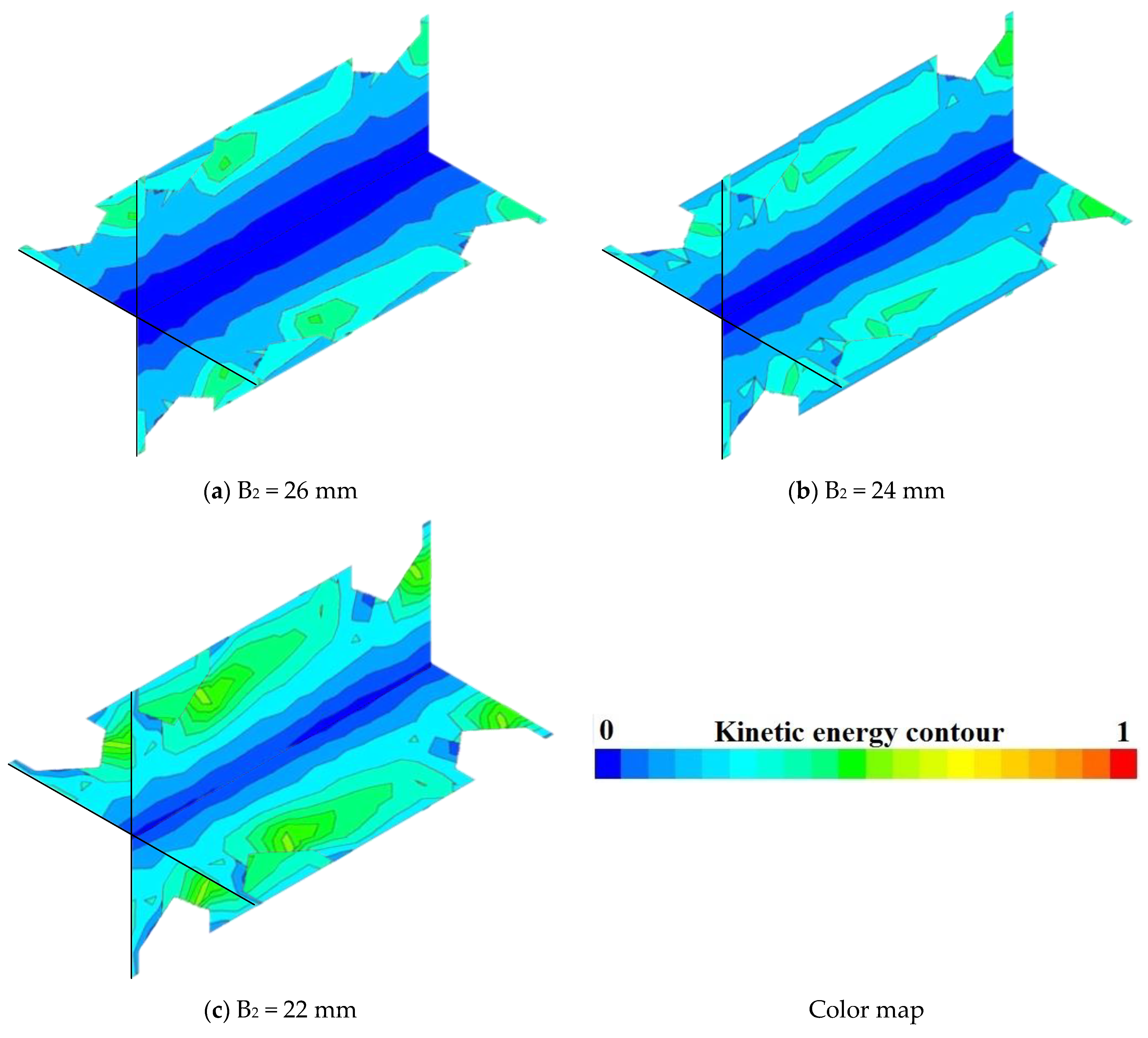
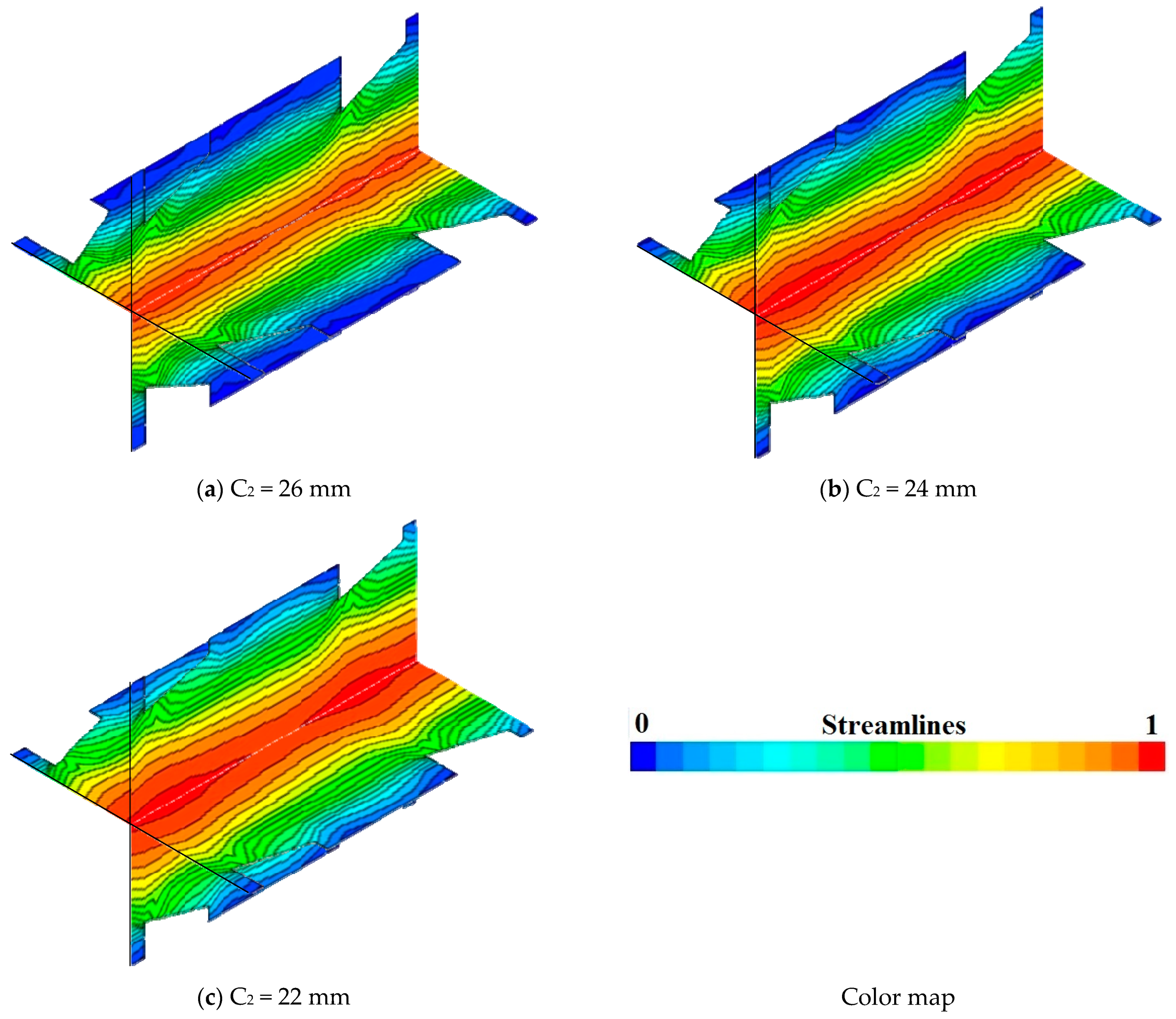
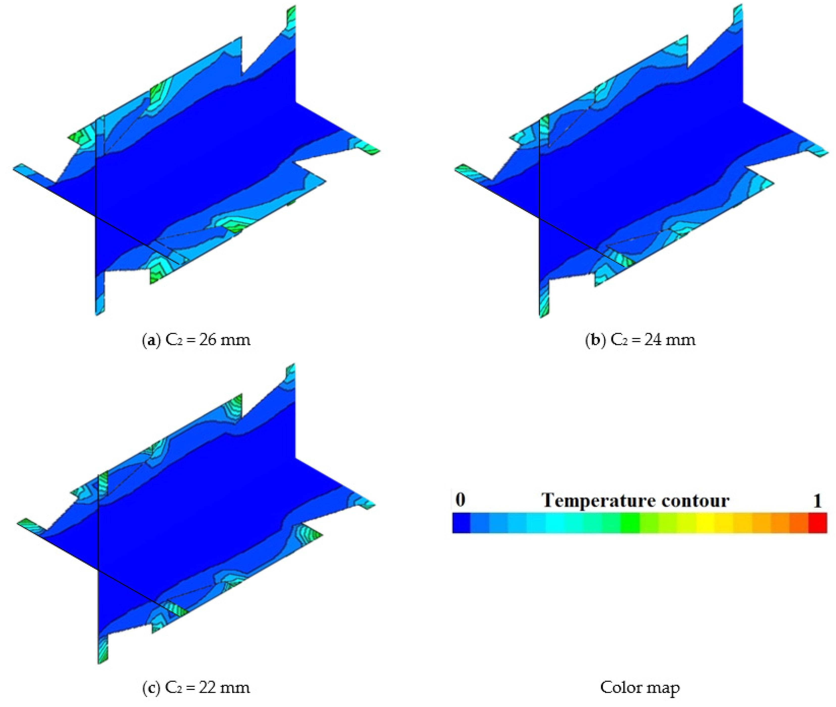
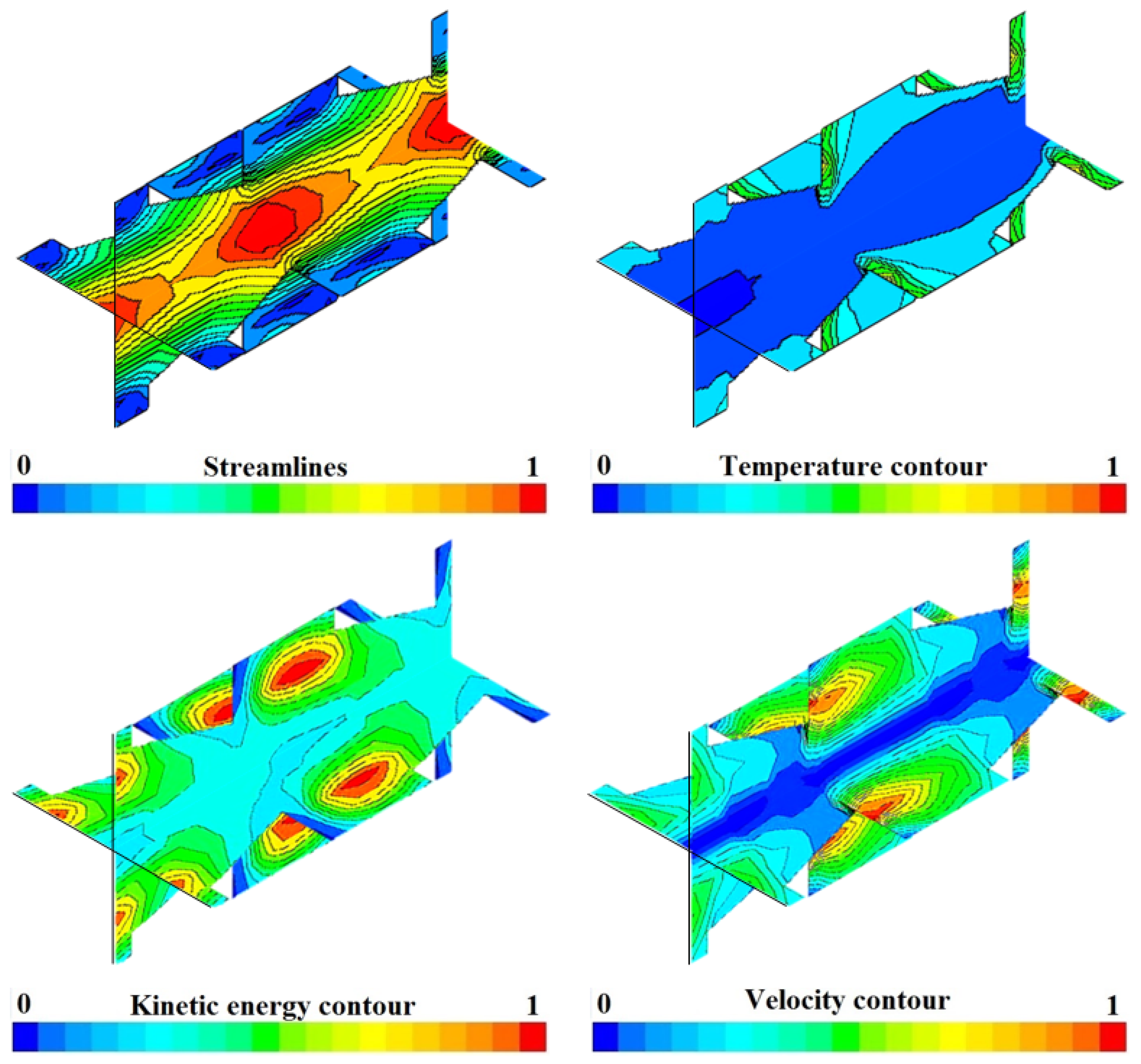
3.3. Case C
3.4. Case D
3.5. Case E
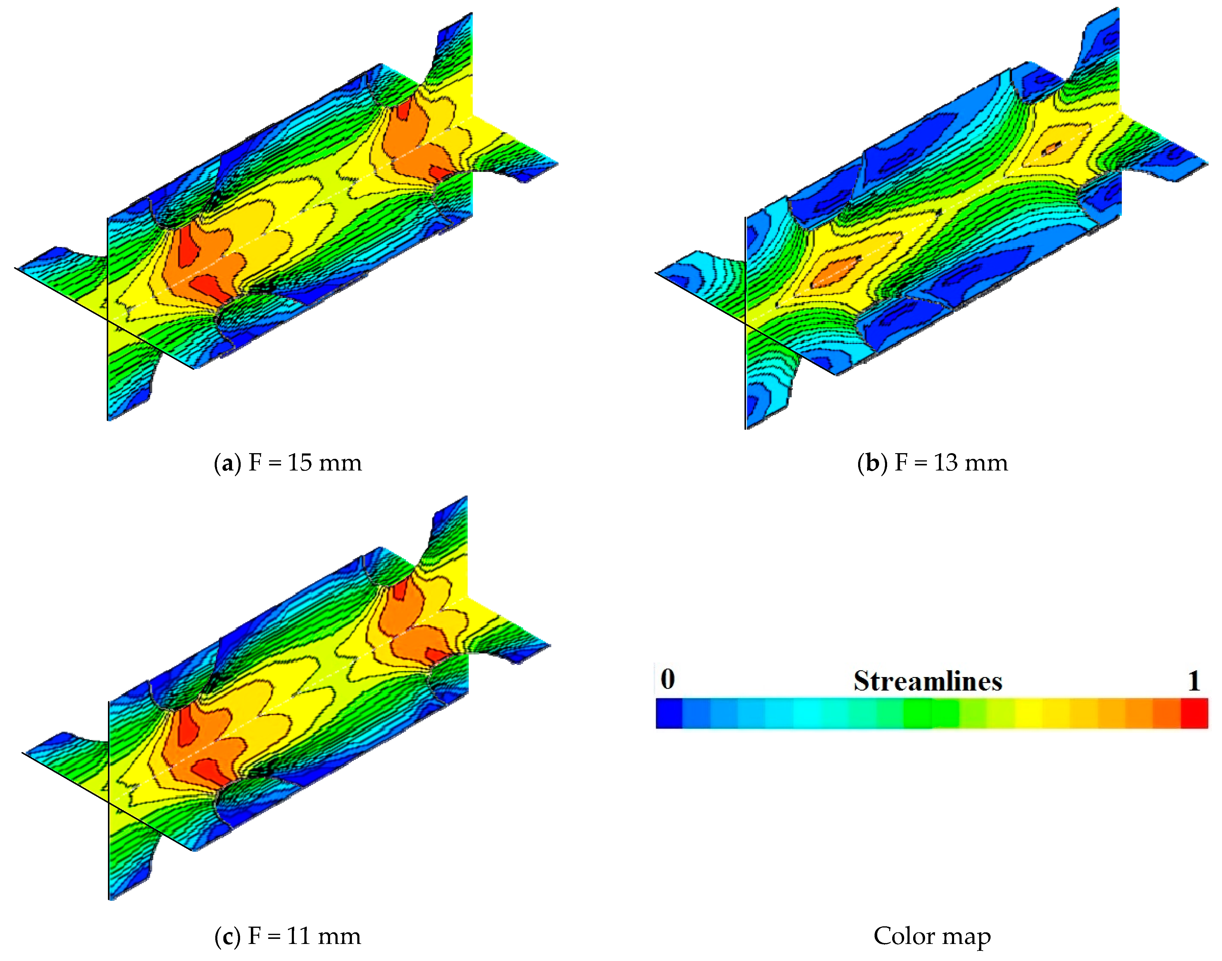
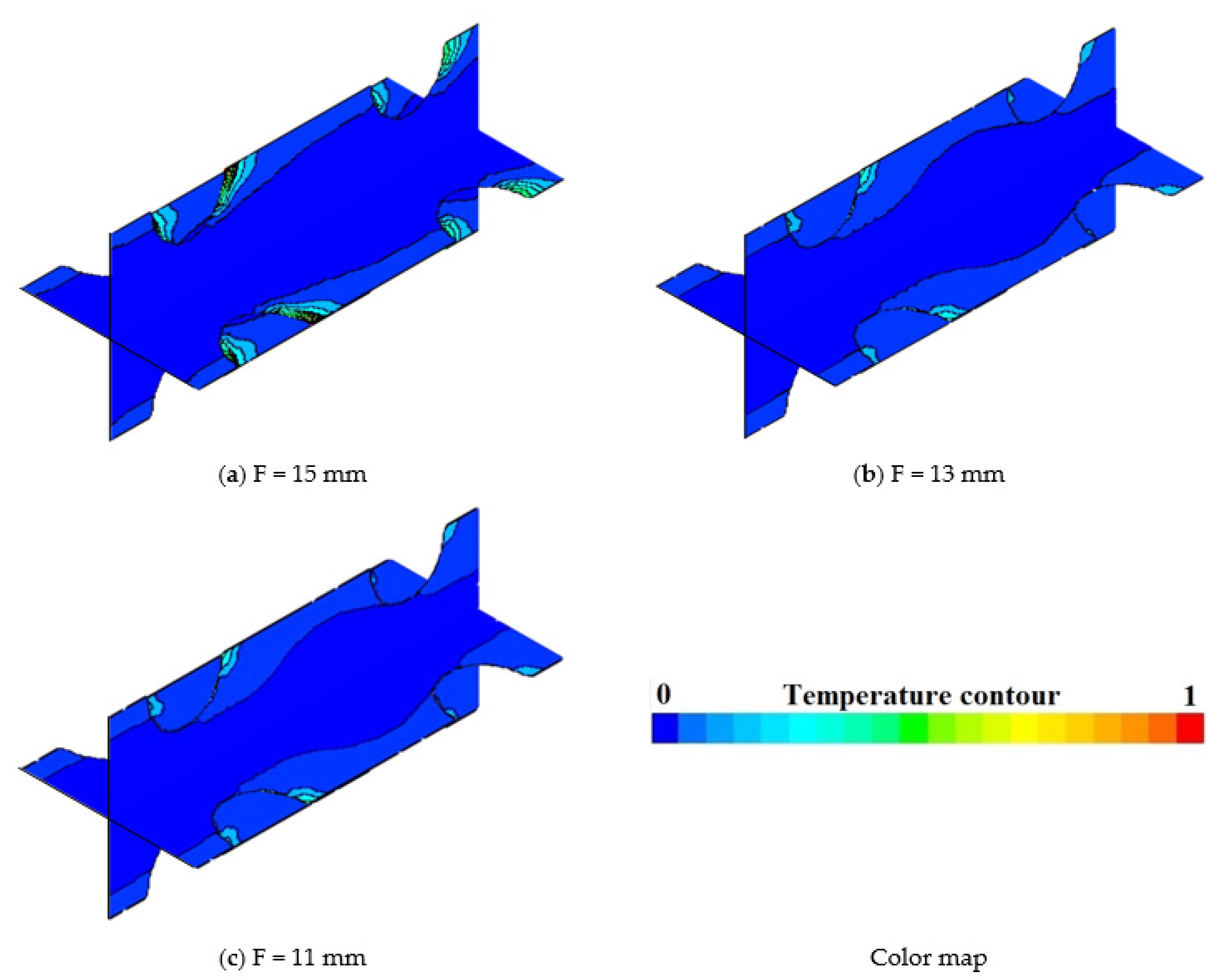
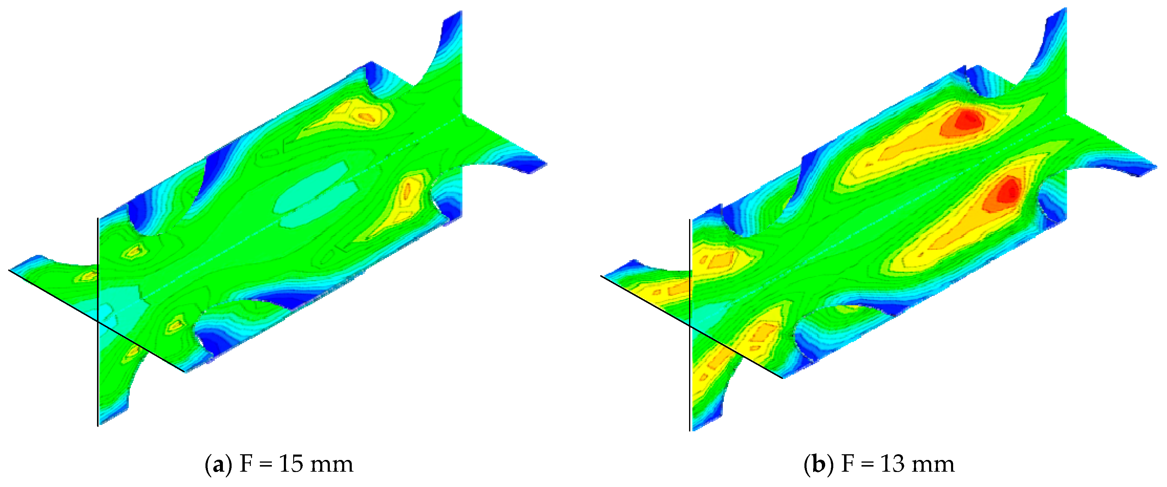
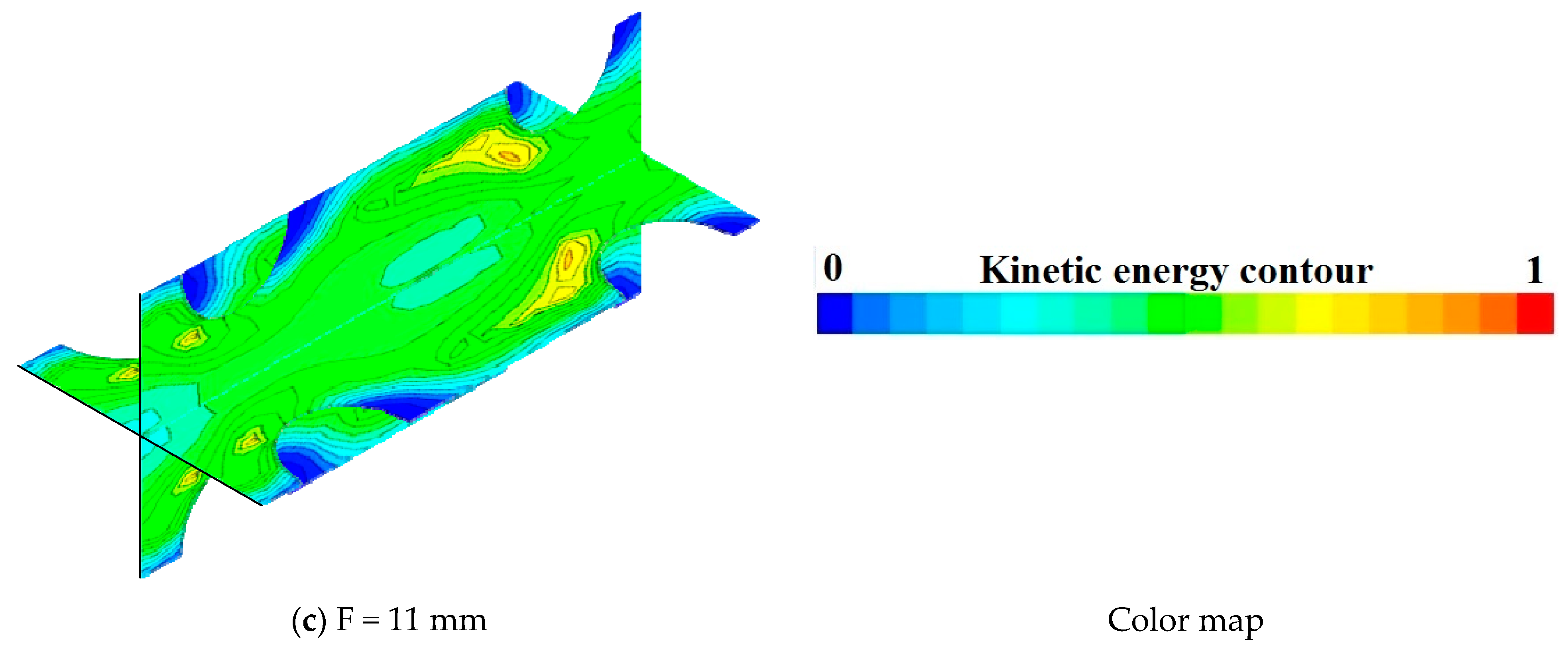
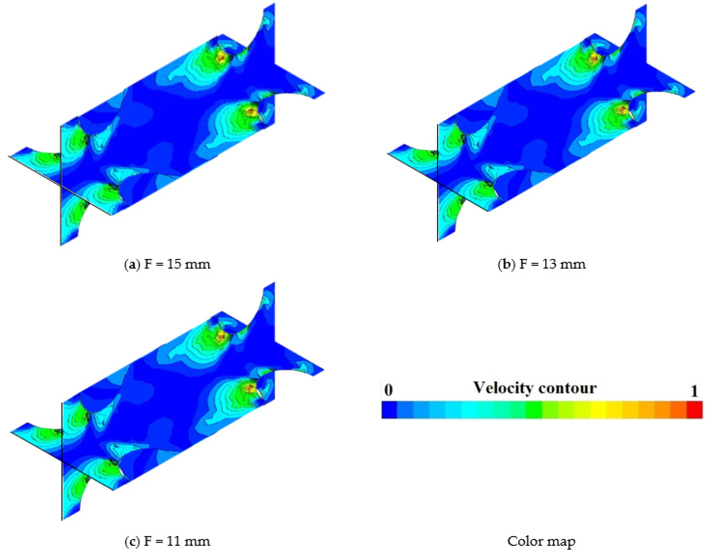
3.6. Case F
3.7. Comparison
- Case A: R = 15 mm and A2 = 24 mm
- Case B: R = 15 mm and B2 = 26 mm
- Case C: R = 13 mm and B2 = 22 mm
- Case D: R = 13 mm and B2 = 24 mm
- Case E: R = 15 mm and B2 = 24 mm
- Case F: F = 15 mm
4. Conclusions
Author Contributions
Funding
Acknowledgments
Conflicts of Interest
Nomenclature
| Specific heat capacity (J/kg.K) | |
| f | Friction coefficient (-) |
| g | Gravitational acceleration (m/s2) |
| Volume fraction | |
| Thermal conductivity (W/m.K) | |
| Nusselt number (-) | |
| Mass-averaged velocity (m/s) | |
| Velocity of solid particles (m/s) | |
| Velocity of the base fluid (m/s) | |
| Drift velocity (m/s) | |
| Greek Symbols | |
| ε | Turbulent dissipation (m2/s3) |
| Efficiency (-) | |
| μ | Viscosity (N·s/m2) |
| Turbulent viscosity (N·s/m2) | |
| Pressure (Pa) | |
| Reynolds number (-) | |
| Subscripts | |
| Nanofluid | |
| Nanoparticle | |
| Solid | |
References
- Parsa, S.M.; Yazdani, A.; Dhahad, H.; Alawee, W.H.; Hesabi, S.; Norozpour, F.; Ali, H.M.; Afrand, M. Effect of Ag, Au, TiO2 metallic/metal oxide nanoparticles in double-slope solar stills via thermodynamic and environmental analysis. J. Clean. Prod. 2021, 311, 127689. [Google Scholar] [CrossRef]
- Eshgarf, H.; Kalbasi, R.; Maleki, A.; Shadloo, M.S.; Karimipour, A. A review on the properties, preparation, models and stability of hybrid nanofluids to optimize energy consumption. J. Therm. Anal. Calorim. 2021, 144, 1959–1983. [Google Scholar] [CrossRef]
- Parsa, S.M.; Rahbar, A.; Koleini, M.; Aberoumand, S.; Afrand, M.; Amidpour, M. A renewable energy-driven thermoelectric-utilized solar still with external condenser loaded by silver/nanofluid for simultaneously water disinfection and desalination. Desalination 2020, 480, 114354. [Google Scholar] [CrossRef]
- Keepaiboon, C.; Dalkilic, A.S.; Mahian, O.; Ahn, H.S.; Wongwises, S.; Mondal, P.K.; Shadloo, M.S. Two-phase flow boiling in a microfluidic channel at high mass flux. Phys. Fluids 2020, 32, 093309. [Google Scholar] [CrossRef]
- Wang, N.; Maleki, A.; Nazari, M.A.; Tlili, I.; Shadloo, M.S. Thermal Conductivity Modeling of Nanofluids Contain MgO Particles by Employing Different Approaches. Symmetry 2020, 12, 206. [Google Scholar] [CrossRef] [Green Version]
- Garbadeen, I.; Sharifpur, M.; Slabber, J.; Meyer, J. Experimental study on natural convection of MWCNT-water nanofluids in a square enclosure. Int. Commun. Heat Mass Transf. 2017, 88, 1–8. [Google Scholar] [CrossRef]
- Rostami, S.; Kalbasi, R.; Talebkeikhah, M.; Goldanlou, A.S. Improving the thermal conductivity of ethylene glycol by addition of hybrid nano-materials containing multi-walled carbon nanotubes and titanium dioxide: Applicable for cooling and heating. J. Therm. Anal. Calorimetry 2021, 143, 1701–1712. [Google Scholar] [CrossRef]
- Yan, S.R.; Golzar, A.; Sharifpur, M.; Meyer, J.P.; Liu, D.H.; Afrand, M. Effect of U-shaped absorber tube on thermal-hydraulic performance and efficiency of two-fluid parabolic solar collector containing two-phase hybrid non-Newtonian nanofluids. Int. J. Mech. Sci. 2020, 185, 105832. [Google Scholar] [CrossRef]
- Aghakhani, S.; Ghasemi, B.; Pordanjani, A.H.; Wongwises, S.; Afrand, M. Effect of replacing nanofluid instead of water on heat transfer in a channel with extended surfaces under a magnetic field. Int. J. Numer. Methods Heat Fluid Flow 2019, 29, 1249–1271. [Google Scholar] [CrossRef]
- Giwa, S.; Sharifpur, M.; Goodarzi, M.; Alsulami, H.; Meyer, J.P. Influence of base fluid, temperature, and concentration on the thermophysical properties of hybrid nanofluids of alumina–ferrofluid: Experimental data, modeling through enhanced ANN, ANFIS, and curve fitting. J. Therm. Anal. Calorim. 2021, 143, 4149–4167. [Google Scholar] [CrossRef]
- Aghakhani, S.; Pordanjani, A.H.; Afrand, M.; Sharifpur, M.; Meyer, J.P. Natural convective heat transfer and entropy generation of alumina/water nanofluid in a tilted enclosure with an elliptic constant temperature: Applying magnetic field and radiation effects. Int. J. Mech. Sci. 2020, 174, 105470. [Google Scholar] [CrossRef]
- Ibrahim, M.; Saeed, T.; Chu, Y.-M.; Ali, H.M.; Cheraghian, G.; Kalbasi, R. Comprehensive study concerned graphene nano-sheets dispersed in ethylene glycol: Experimental study and theoretical prediction of thermal conductivity. Powder Technol. 2021, 386, 51–59. [Google Scholar] [CrossRef]
- Pordanjani, A.H.; Aghakhani, S.; Afrand, M.; Mahmoudi, B.; Mahian, O.; Wongwises, S. An updated review on application of nanofluids in heat exchangers for saving energy. Energy Convers. Manag. 2019, 198, 111886. [Google Scholar] [CrossRef]
- Komeilibirjandi, A.; Raffiee, A.H.; Maleki, A.; Nazari, M.A.; Shadloo, M.S. Thermal conductivity prediction of nanofluids containing CuO nanoparticles by using correlation and artificial neural network. J. Therm. Anal. Calorim. 2020, 139, 2679–2689. [Google Scholar] [CrossRef]
- Pordanjani, A.H.; Aghakhani, S. Numerical Investigation of Natural Convection and Irreversibilities between Two Inclined Concentric Cylinders in Presence of Uniform Magnetic Field and Radiation. Heat Transf. Eng. 2021, 1–21. [Google Scholar] [CrossRef]
- Yan, S.-R.; Aghakhani, S.; Karimipour, A. Influence of a membrane on nanofluid heat transfer and irreversibilities inside a cavity with two constant-temperature semicircular sources on the lower wall: Applicable to solar collectors. Phys. Scr. 2020, 95, 085702. [Google Scholar] [CrossRef]
- Ghalandari, M.; Maleki, A.; Haghighi, A.; Shadloo, M.S.; Nazari, M.A.; Tlili, I. Applications of nanofluids containing carbon nanotubes in solar energy systems: A review. J. Mol. Liq. 2020, 313, 113476. [Google Scholar] [CrossRef]
- Parsa, S.M. Reliability of thermal desalination (solar stills) for water/wastewater treatment in light of COVID-19 (novel coronavirus “SARS-CoV-2”) pandemic: What should consider? Desalination 2021, 512, 115106. [Google Scholar] [CrossRef]
- Rostami, S.; Aghakhani, S.; Pordanjani, A.H.; Afrand, M.; Cheraghian, G.; Oztop, H.F.; Shadloo, M.S. A Review on the Control Parameters of Natural Convection in Different Shaped Cavities with and Without Nanofluid. Processes 2020, 8, 1011. [Google Scholar] [CrossRef]
- Parsa, S.M.; Rahbar, A.; Koleini, M.; Javadi, Y.D.; Afrand, M.; Rostami, S.; Amidpour, M. First approach on nanofluid-based solar still in high altitude for water desalination and solar water disinfection (SODIS). Desalination 2020, 491, 114592. [Google Scholar] [CrossRef]
- Nakharintr, L.; Naphon, P. Magnetic field effect on the enhancement of nanofluids heat transfer of a confined jet impingement in mini-channel heat sink. Int. J. Heat Mass Transf. 2017, 110, 753–759. [Google Scholar] [CrossRef]
- Ashorynejad, H.R.; Zarghami, A. Magnetohydrodynamics flow and heat transfer of Cu-water nanofluid through a partially porous wavy channel. Int. J. Heat Mass Transf. 2018, 119, 247–258. [Google Scholar] [CrossRef]
- Dormohammadi, R.; Farzaneh-Gord, M.; Ebrahimi-Moghadam, A.; Ahmadi, M.H. Heat transfer and entropy generation of the nanofluid flow inside sinusoidal wavy channels. J. Mol. Liq. 2018, 269, 229–240. [Google Scholar] [CrossRef]
- Saeed, M.; Kim, M.-H. Heat transfer enhancement using nanofluids (Al2O3-H2O) in mini-channel heatsinks. Int. J. Heat Mass Transf. 2018, 120, 671–682. [Google Scholar] [CrossRef]
- Dalkılıç, A.S.; Türk, O.A.; Mercan, H.; Nakkaew, S.; Wongwises, S. An experimental investigation on heat transfer characteristics of graphite-SiO2/water hybrid nanofluid flow in horizontal tube with various quad-channel twisted tape inserts. Int. Commun. Heat Mass Transf. 2019, 107, 1–13. [Google Scholar] [CrossRef]
- Saba, F.; Ahmed, N.; Khan, U.; Mohyud-Din, S.T. A novel coupling of (CNT-Fe3O4/H2O) hybrid nanofluid for improvements in heat transfer for flow in an asymmetric channel with dilating/squeezing walls. Int. J. Heat Mass Transf. 2019, 136, 186–195. [Google Scholar] [CrossRef]
- Ajeel, R.K.; Salim, W.I.; Hasnan, K. Experimental and numerical investigations of convection heat transfer in different channels using alumina nanofluid under a turbulent flow regime. Chem. Eng. Res. Des. 2019, 148, 202–217. [Google Scholar] [CrossRef]
- Gholami, M.; Nazari, M.R.; Talebi, M.H.; Pourfattah, F.; Akbari, O.A.; Toghraie, D. Natural convection heat transfer enhancement of different nanofluids by adding dimple fins on a vertical channel wall. Chin. J. Chem. Eng. 2020, 28, 643–659. [Google Scholar] [CrossRef]
- Shah, Z.; Khan, A.; Khan, W.; Alam, M.K.; Islam, S.; Kumam, P.; Thounthong, P. Micropolar gold blood nanofluid flow and radiative heat transfer between permeable channels. Comput. Methods Programs Biomed. 2020, 186, 105197. [Google Scholar] [CrossRef]
- Ajeel, R.K.; Salim, W.I.; Sopian, K.; Yusoff, M.Z.; Hasnan, K.; Ibrahim, A.; Al-Waeli, A.H. Turbulent convective heat transfer of silica oxide nanofluid through different channels: An experimental and numerical study. Int. J. Heat Mass Transf. 2019, 145, 118806. [Google Scholar] [CrossRef]
- Ajeel, R.K.; Salim, W.S.I.W.; Hasnan, K. Influences of geometrical parameters on the heat transfer characteristics through symmetry trapezoidal-different channel using SiO2-water nanofluid. Int. Commun. Heat Mass Transf. 2019, 101, 1–9. [Google Scholar] [CrossRef]
- Ajeel, R.K.; Salim, W.I.; Hasnan, K. Numerical investigations of heat transfer enhancement in a house shaped-different channel: Combination of nanofluid and geometrical parameters. Therm. Sci. Eng. Prog. 2020, 17, 100376. [Google Scholar] [CrossRef]
- Salimpour, M.R.; Kalbasi, R.; Lorenzini, G. Constructal multi-scale structure of PCM-based heat sinks. Contin. Mech. Thermodynamics 2017, 29, 477–494. [Google Scholar] [CrossRef]
- Salari, A.; Kazemian, A.; Ma, T.; Hakkaki-Fard, A.; Peng, J. Nanofluid based photovoltaic thermal systems integrated with phase change materials: Numerical simulation and thermodynamic analysis. Energy Convers. Manag. 2020, 205, 112384. [Google Scholar] [CrossRef]
- Al-Ansary, H.; Zeitoun, O. Numerical study of conduction and convection heat losses from a half-insulated air-filled annulus of the receiver of a parabolic trough collector. Sol. Energy 2011, 85, 3036–3045. [Google Scholar] [CrossRef]
- Arani, A.A.A.; Sadripour, S.; Kermani, S. Nanoparticle shape effects on thermal-hydraulic performance of boehmite alumina nanofluids in a sinusoidal–wavy mini-channel with phase shift and variable wavelength. Int. J. Mech. Sci. 2017, 128–129, 550–563. [Google Scholar] [CrossRef]
- Sadripour, S. 3D numerical analysis of atmospheric-aerosol/carbon-black nanofluid flow within a solar air heater located in Shiraz, Iran. Int. J. Numer. Methods Heat Fluid Flow 2018, 29, 1378–1402. [Google Scholar] [CrossRef]
- Sadripour, S.; Chamkha, A.J. The effect of nanoparticle morphology on heat transfer and entropy generation of supported nanofluids in a heat sink solar collector. Therm. Sci. Eng. Prog. 2019, 9, 266–280. [Google Scholar] [CrossRef]
- Kim, D.; Kwon, Y.; Cho, Y.; Li, C.; Cheong, S.; Hwang, Y.; Lee, J.; Hong, D.; Moon, S. Convective heat transfer characteristics of nanofluids under laminar and turbulent flow conditions. Curr. Appl. Phys. 2009, 9, e119–e123. [Google Scholar] [CrossRef]
- Giwa, S.; Sharifpur, M.; Meyer, J. Experimental study of thermo-convection performance of hybrid nanofluids of Al2O3-MWCNT/water in a differentially heated square cavity. Int. J. Heat Mass Transf. 2020, 148, 119072. [Google Scholar] [CrossRef]
- Leong, W.; Hollands, K.; Brunger, A. Experimental Nusselt numbers for a cubical-cavity benchmark problem in natural convection. Int. J. Heat Mass Transf. 1999, 42, 1979–1989. [Google Scholar] [CrossRef]
- Yang, S.; Ordonez, J. 3D thermal-hydraulic analysis of a symmetric wavy parabolic trough absorber pipe. Energy 2019, 189, 116320. [Google Scholar] [CrossRef]


| Parameters | Values | Parameters | Values |
|---|---|---|---|
| D | 60 mm | J | 17 mm |
| L | R | 11, 13 and 15 mm | |
| A1 | 12 mm | A2 | 22, 24 and 26 mm |
| B1 | 12 mm | B2 | 22, 24 and 26 mm |
| C1 | 12 mm | C2 | 22, 24 and 26 mm |
| D1 | 12 mm | D2 | 22, 24 and 26 mm |
| E1 | 12 mm | E2 | 10, 12 and 14 mm |
| F | 11, 13 and 15 mm | 2 mm | |
| Tin | 330 K | Ts | 450 K |
| Pout | 0 (gage) | Re | 11,000, 15,000, 19,000, and 23,000 |
| Thermophysical Properties | k (W/m·K) | cp (J/kg·K) | ρ (kg/m3) | Mean Diameter of Particle (nm) |
|---|---|---|---|---|
| Graphite | 25 | 720 | 2060 | 8 |
| SiO2 | 1.4 | 765 | 2200 | 7 |
| water | 0.613 | 4179 | 997.1 | - |
Publisher’s Note: MDPI stays neutral with regard to jurisdictional claims in published maps and institutional affiliations. |
© 2021 by the authors. Licensee MDPI, Basel, Switzerland. This article is an open access article distributed under the terms and conditions of the Creative Commons Attribution (CC BY) license (https://creativecommons.org/licenses/by/4.0/).
Share and Cite
Khetib, Y.; Alahmadi, A.; Alzaed, A.; Tahmasebi, A.; Sharifpur, M.; Cheraghian, G. Effects of Different Wall Shapes on Thermal-Hydraulic Characteristics of Different Channels Filled with Water Based Graphite-SiO2 Hybrid Nanofluid. Processes 2021, 9, 1253. https://0-doi-org.brum.beds.ac.uk/10.3390/pr9071253
Khetib Y, Alahmadi A, Alzaed A, Tahmasebi A, Sharifpur M, Cheraghian G. Effects of Different Wall Shapes on Thermal-Hydraulic Characteristics of Different Channels Filled with Water Based Graphite-SiO2 Hybrid Nanofluid. Processes. 2021; 9(7):1253. https://0-doi-org.brum.beds.ac.uk/10.3390/pr9071253
Chicago/Turabian StyleKhetib, Yacine, Ahmad Alahmadi, Ali Alzaed, Ahamd Tahmasebi, Mohsen Sharifpur, and Goshtasp Cheraghian. 2021. "Effects of Different Wall Shapes on Thermal-Hydraulic Characteristics of Different Channels Filled with Water Based Graphite-SiO2 Hybrid Nanofluid" Processes 9, no. 7: 1253. https://0-doi-org.brum.beds.ac.uk/10.3390/pr9071253