Automated Compartment Model Development Based on Data from Flow-Following Sensor Devices

Abstract

Due to the heterogeneous nature of large-scale fermentation processes they cannot be modelled as ideally mixed reactors, and therefore flow models are necessary to accurately represent the processes. Computational fluid dynamics (CFD) is used more and more to derive flow fields for the modelling of bioprocesses, but the computational demands associated with simulation of multiphase systems with biokinetics still limits their wide applicability. Hence, a demand for simpler flow models persists. In this study, an approach to develop data-based flow models in the form of compartment models is presented, which utilizes axial-flow rates obtained from flow-following sensor devices in combination with a proposed procedure for automatic zoning of volume. The approach requires little experimental effort and eliminates the necessity for computational determination of inter-compartmental flow rates and manual zoning. The concept has been demonstrated in a 580 L stirred vessel, of which models have been developed for two types of impellers with varying agitation intensities. The sensor device measurements were corroborated by CFD simulations, and the performance of the developed compartment models was evaluated by comparing predicted mixing times with experimentally determined mixing times. The data-based compartment models predicted the mixing times for all examined conditions with relative errors in the range of 3–27%. The deviations were ascribed to limitations in the flow-following behavior of the sensor devices, whose sizes were relatively large compared to the examined system. The approach provides a versatile and automated flow modelling platform which can be applied to large-scale bioreactors.

1. Introduction

In the biotechnology industry models serve as an important tool to improve process efficiency and to provide a quantitative basis for process optimization, design, and control [1]. The environment of fermentation broths in industrial bioreactors is heterogeneous [2], and therefore models of microbial kinetics must be accompanied by liquid flow models to provide an accurate representation of the system [3]. These flow models are often developed based on the compartment model approach or with the use of computational fluid dynamics [4].

Computational fluid dynamics (CFD) comprises a collection of advanced modelling techniques which can provide detailed modelling of the hydrodynamics in bioreactors [5]. However, CFD is associated with considerable computational demands, which limits its wide application for the simulation of fermentation processes, where microbial reactions are considered [6]. Furthermore, predictions of multiphase and/or viscous systems, which is often the reality in fermentation processes, may suffer from modelling errors [6,7]. This poses a problem because the acquisition of spatial velocity measurements, which are needed for validation of the models, is challenging in industrial bioreactors [8,9].

Compartment modelling (CM) provides a simpler and less computationally demanding approach, in which flows are defined between a network of ideally mixed zones called compartments. With compartment models the modeler must make decisions regarding the number of compartments, the volumes of the compartments, the connections between the compartments, and the flow rates between them. The accuracy of the resulting model is highly dependent on these decisions [10]; Hence, unless the decisions are automated programmatically the model performance depends on the experience of the modeler. The traditional approach to compartment models is to support these decisions by knowledge from gross flow patterns, which have been extensively studied [11], and calculate the flow rates between the compartments with empirical correlations and experimentally determined global quantities, such as dimensionless flow numbers. Models of this type have been developed for both stirred tank bioreactors and for bubble-column bioreactors [4,8,12,13] and have been shown to provide reasonable predictions for mixing in stirred bioreactors with and without aeration [4,8]. The empirical nature and the use of global quantities in this approach makes it difficult to accurately determine the flow rates between adjacent compartments in the entire flow field, and thus the adaptability of the models to various bioreactor configurations is limited. A more recent approach is to compute the flows from the velocity fields obtained by CFD simulations with different zoning approaches of varying complexity [6,10,14,15]. This enables trading reduced model accuracy for a shortened computation time. However, CFD-based compartment models still inherit the previously mentioned limitations of CFD with respect to challenges with multiphase and viscous systems, and the lack of validation of the models in industrial bioreactors. A third option is an entirely data-based approach, which will be presented in this paper. The approach is enabled by the Lagrangian measurement technology of flow-following sensor devices, which have been introduced in earlier studies as a practical method to obtain axial velocity fields from bioreactors [9]. These axial velocity fields can be exploited in the development of compartment models.

The contribution of this paper is a methodology for developing compartment models based on axial velocities, derived from pressure measurements collected by flow-following sensor devices. The methodology can be broken down into two fundamental steps. First, determination of inter-compartmental flow rates between a set of equally spaced compartments which together represents the vessel volume. These compartments are referred to as initial compartments. Secondly, merging of the initial compartments into a set of perfectly mixed compartments in a process referred to as automatic zoning. The validity of the fundamental assumption for determining the flow rates between the compartments is corroborated by results from CFD simulations, and compartment model predictions of mixing times are compared against experimental data.

2. Materials and Methods

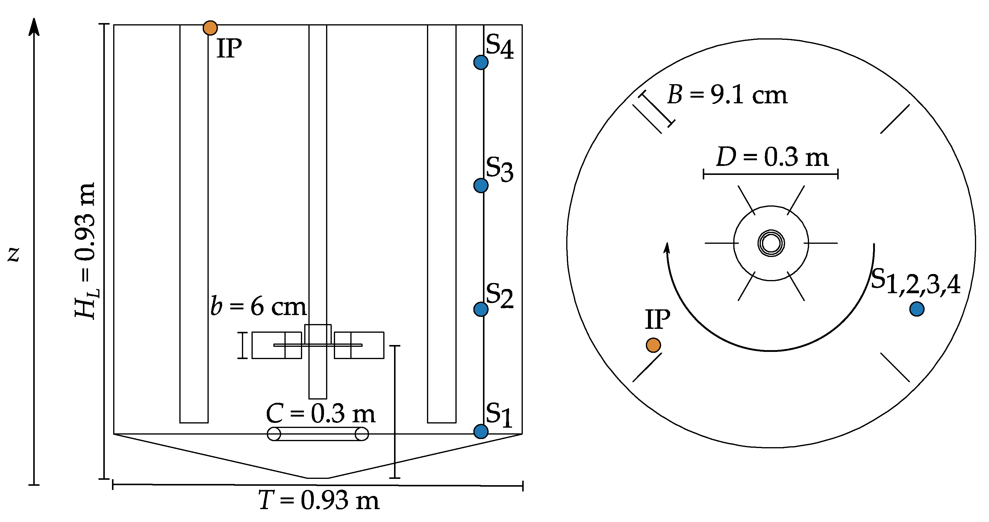
2.1. Stirred Reactor Geometry

The experiments were performed in a pilot-scale stirred vessel with a truncated conical bottom. The diameter of the vessel was T = 0.93 m, and the vessel was equipped with four baffles with a width of B = 9.1 cm. The geometry is outlined in Figure 1, together with details about the relevant dimensions. Besides the annotated geometries, a ring sparger with a diameter of 20 cm is located 10 cm above the bottom of the vessel.

2.2. Experimental Conditions

The examined conditions include agitation by a radial impeller (6-bladed Rushton disc turbine, RDT) and a down-pumping mixed-flow impeller with a predominant axial flow (45° 4-bladed pitched-blade turbine, PBT). Both impeller types were of the same dimensions, having a diameter of D = 0.3 m and a blade height of b = 6 cm. The experiments were carried out at four levels of specific power input, ε₁ = 0.02, ε₂ = 0.11, ε₃ = 0.21 and ε₄ = 0.31 W/kg. The four levels of specific power input correspond to impeller speeds of N = 60, 105, 130 and 150 rpm in the case of the radial impeller, and N = 105, 175, 220 and 245 rpm, in the case of the axial impeller. The experiments were carried out in demineralized water at room temperature (ρ_l = 998 kg/m³). The Reynolds number of the examined conditions, which was calculated by Re = ρ_fND²/µ, ranges from of Re = 9∙× 10⁴ to Re = 4∙× 10⁵ and the flow is therefore expected to be fully turbulent. A working volume of V = 580 L was used for all the experiments, resulting in a liquid height of H_L = 0.93 and an aspect ratio of H_L/T = 1.

2.3. Mixing Time

The pulse responses for determination of the mixing time were obtained by injection of alternating pulses of 50 wt% sodium hydroxide (NaOH) and 50 wt% sulfuric acid (H₂SO₄) in demineralized water. The system was buffered with 2 mM succinic acid and 2 mM malonic acid, which produces a linear pH response between pH 3 and 6 [16]. The pulses were added slightly to the side of the baffle at the top of the liquid, at the injection point (IP) shown in Figure 1. To pump the acid and base, two diaphragm pumps (Xylem Flojet Model: RLF122002C) were used. Injections of approximately 160 mL of H₂SO₄ and 100 mL of NaOH were used to generate pulses of approximately 1 pH unit. This resulted in pumping times of 2.8 and 1.8 s for the acid and base, respectively, which were subtracted from the corresponding mixing time calculations. After each tracer injection, the system was allowed to stabilize for four minutes before the next tracer pulse was injected. After the four minutes, the tracer was considered completely homogenized. The responses of seven pulses were captured by four fixed pH sensors (Figure 1, Tables S1 and S2) with short response times of less than 5 s (Endress + Hauser CPS471D-7211), located at z/H_L = 0.11, 0.38, 0.65 and 0.91. The 95% mixing time (t_m,95), which is defined as the time it takes for the tracer concentration to reach 95% of the concentration at complete homogenization, was calculated from the logarithmic root-mean-square (RMS) variance of the normalized responses from all four sensors, according to the procedure described in [17].

2.4. Flow-Following Sensor Devices

Flow-following sensor devices (Fermsense 3D, Freesense ApS [18,19]) were deployed to collect pressure measurements during the experiments. The sensor devices, measuring 43 mm in diameter, were configured to collect measurements at a sampling frequency of 8 Hz. The mass of each sensor device was adjusted to 41.6 g, which was calculated based on the volume of a perfect sphere in order to match the density of water at room temperature (ρ_l = 998 kg/m³). The data sets for each of the experimental conditions are comprised of one hour of continuous pressure measurements from four sensor devices. The pressure sensor has the following specifications: a measurement range of 1–5 bar, an accuracy ±10 mbar (20–60 °C), a resolution of 0.38 mbar and a response time of 10 ms (t₉₀). The accuracy is not critical for the experiments, as only the pressure difference between the sensor device and the liquid surface is of interest, which can easily be inferred from the measurements. A resolution of 0.38 mbar enables the detection of changes in the liquid column height above the sensor device of 0.39 cm, which is sufficient to resolve the 0.93 m liquid height in detail.

Processing of Sensor Device Data

The pressure signal was filtered with a rolling median filter with a window size of three samples to remove unwanted spikes which occurred when the sensor devices impacted with the impeller. The signal was then filtered by a three-sample rolling average filter to reconstruct a smooth profile. In order to obtain the axial position time series of the sensor devices (z(t)), the pressure measurements were converted by first subtracting the maximum measured pressure, corresponding to the bottom of the vessel, and then applying Pascal’s principle (Equation (1)), on the resulting pressure differences (ΔP(t)).

$$z\left(t\right)=\frac{\mathsf{\Delta }P\left(t\right)}{{\rho }_f\cdot g}$$

(1)

Axial velocities (v_z(t)) in the vessel were then obtained from the time derivative of the axial position, which results in both positive and negative velocities, corresponding to the upwards and downwards movements of the sensor devices.

Axial velocities over the compartment interfaces were isolated by deriving linear regressions of each pair of axial position measurements, z(t) = v_zt + b, assuming a constant velocity between the measurements. This is a reasonable assumption as the sampling frequency of eight samples per second is high compared to the magnitudes of the velocities in the system. The equations were solved for b and z(t) was replaced by a detection plane, z_plane, to solve for t, corresponding to the intersection time, t_x, if t_i−1 ≤ t_x ≤ t_i. In the stirred vessel, the value z_plane corresponds to a horizontal plane representing an interface between two adjacent compartments. The axial velocities over each z_plane, i.e., the slopes of the lines when t = t_x, were then separated into negative and positive values and averaged to obtain the final average upwards velocity (${\overline{v}}_{z,up}$) and downwards velocity (${\overline{v}}_{z,down}$) over the interfaces.

3. Modelling

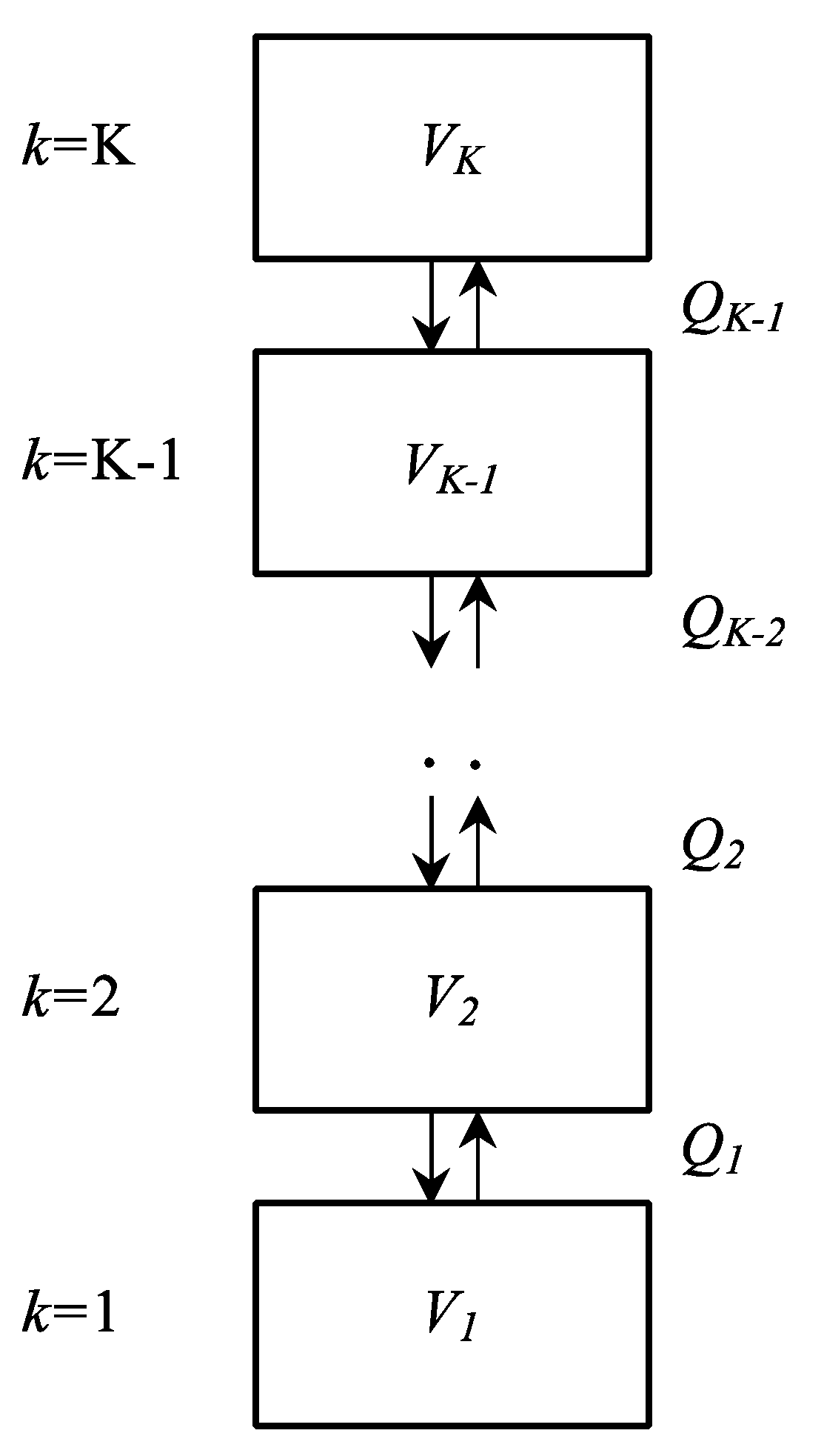
3.1. Data-Based Axial Compartment Model

The compartment model (CM) comprises of bidirectional axial exchanges of mass with a given flow rate (Q_k), between a set of ideally mixed compartments (k = 1, …, K) with equal or differing volumes (V_k). A simple schematic representation of the compartment model is shown in Figure 2.

The sole employment of axial compartments in the model implies that perfect radial mixing within the compartments is assumed. The differential equations constituting the compartment models are derived from the mass balances of ideally mixed compartments in Equations (2)–(4).

$$V_1\frac{d{C}_1}{dt}=C_2{Q}_1-C_1{Q}_1$$

(2)

$$V_k\frac{d{C}_k}{dt}=C_{k-1}{Q}_{k-1}+C_{k+1}{Q}_k-C_k{Q}_{k-1}-C_k{Q}_k,k=2,\dots ,K-1$$

(3)

$$V_K\frac{d{C}_K}{dt}=C_{K-1}{Q}_{K-1}-C_K{Q}_{K-1}$$

(4)

3.1.1. Inter-Compartmental Flow Rates and Volumes

The volumetric flows (Q) between the compartments are calculated from the vessel diameter (T) and the linear averaged axial velocities in the upwards direction (${\overline{v}}_{z,up}$) and downwards direction (${\overline{v}}_{z,down}$), by solving for the cross-sectional area of the fluid moving upwards ($A_{up}$) and downwards ($A_{down}$) in Equations (5)–(7):

$$Q_k={\overline{v}}_{z,up\left(k\right)}\cdot A_{up\left(k\right)}={\overline{v}}_{z,down\left(k\right)}\cdot A_{down\left(k\right)}$$

(5)

$$A=A_{up\left(k\right)}+A_{down\left(k\right)}$$

(6)

$$A=\frac{\pi T^2}{4}$$

(7)

The compartment volumes (V_k) are calculated as cylindric volumes with heights corresponding to the differences between the heights of the compartment interfaces. The volumes at the conical bottom are approximated by cylinders, using the area from the vessel geometry at the center of the compartments.

3.1.2. Automatic Zoning

The proposed automatic zoning approach is based on the volume to flow-rate ratio (V/Q) in the compartments. This definition is similar to the definition of residence time (τ) in a chemostat [20] and similarly the ratio describes the time it takes to replace the entire volume in a compartment by an external volume, as it applies for each compartment that Q_in = Q_out. It is reasoned that a critical local residence time (τ_crit) can be defined, for which this ratio indicates whether the assumption about perfect mixing is acceptable, although this ratio is strictly zero for a perfectly mixed compartment. The volume is initially divided into a set of smaller sub-compartments (K_init) from which the zoning algorithm iteratively merges compartments. Starting from the bottom compartment (k = 1), the compartment is tested for the condition stated in Equation (8).

$$\tau =\frac{V}{Q}\le {\tau }_{crit}$$

(8)

For two or more compartments to merge, they need to satisfy the condition individually and with their volumes combined. When the volumes are combined, the flow rates entering this combined compartment volume are used. If the condition is not satisfied for a compartment, the compartment is left unchanged from its initial state. For the merging of n out of K compartments, the condition can be written as in Equation (9).

$$\frac{{{\displaystyle \sum }}_k^{k+n-1}{V}_k}{Q_{k-1}+Q_{k+n-1}}\le {\tau }_{crit},$$

(9)

where the flow rates entering and leaving the outer compartments, Q₀ and Q_K, are set to zero.

The initial number of compartments was chosen to K_init = 25. For K_init > 10, the optimal value for τ_crit was found to be independent of the initial number of compartments, while minor reductions in model error were found when increasing from K_init = 10 to K_init = 25. As the automatic zoning is based on merging of the initial compartments at their interfaces, a larger model error when K_init < 10 can be explained by insufficient initial interfaces for the merging algorithm. Sufficient interfaces are necessary to obtain small compartments at volumes with poor mixing and to have interfaces available at important locations, for example, where the direction of the axial flow changes. If too many initial compartments are chosen (K_init is very large), the initial compartments will be very small. Very small compartments at zones with little sensor device presence face the risk that the average axial velocity has not converged to a stable value because the experiment duration, and therefore the velocity sample size, are confined in practice. This situation can be prevented by collecting more data by either deploying more sensor devices or examining a steady flow field for a longer duration.

The value for the parameter τ_crit was obtained by minimizing the sum of squared errors (SSE) between the measured mean mixing times and the simulated mixing times of the eight experimental conditions (four agitation levels with two impeller types). The simulated mixing times refer to the predictions from the compartment models developed based on flow rates obtained from the flow-following sensor devices. The parameter τ_crit is indirectly related to the mixing time, such that when τ_crit is increased more compartments are merged, resulting in larger compartments. Larger compartments imply that larger volumes are assumed to be perfectly mixed, and therefore the mixing time decreases. The opposite is true for reductions of τ_crit, which results in smaller compartments and longer mixing times.

3.2. Simulation of Tracer Pulses

The tracer concentration transients were simulated by initializing an arbitrary tracer concentration in the top compartment and numerically solving the ordinary differential equations (Equations (1)–(3)) using the LSODA solver implementation from Python’s Scipy library. The time to reach 95% homogeneity (t_m95) was determined from the logarithmic RMS variance of the normalized responses in all the modelled compartments.

3.3. CFD Simulations

The RDT and the PBT configurations were examined using CFD, with the geometry of the volume (Figure 1) generated in SolidWorks 2018. The vessel geometries with the RDT and the PBT were discretized in ICEM CFX 19.2 using a structured hexahedral mesh with an average mesh density of 2100 elements/L in the bulk (stationary domain). For the impeller area of the RDT (rotating domain), a structured hexahedral mesh with an average mesh density of 6200 elements/L was used, while for the PBT, an unstructured tetrahedral mesh with average mesh density of 7900 elements/L was used. The generated mesh densities are comparable with other similar studies [21]. The distribution of elements located at the rotating/stationary interface is matched to avoid local numerical instability. A mesh convergence study was performed to investigate model independence on mesh density. Refer to “Supplementary Materials” for mesh study results and details of the mesh generation.

The simulations were set up in ANSYS CFX 19.2 by employing the standard RANS k-ε turbulent model. The interfaces between the rotating and stationary domains were set as Transient Rotor-Stator interface with ‘automatic pitch change’. The liquid flow at the defined walls in the geometry, consisting of liquid surface and the solid surfaces in the vessel, i.e., the vessel walls, the impeller, the baffles, and the sparger, was solved using no-slip boundary condition. An open boundary was used for the liquid surface. Finally, the liquid profiles were calculated using the second order backwards Eulerian approach. An RMS residual level of 10⁻⁴ was used as the convergence criterion for the solutions.

For the comparative analysis of flow rates between the compartments obtained from CFD and from sensor device measurements, data on the axial velocity and the area were extracted from the mesh cells of 20 equally distributed planes in the axial direction. The overall flow rates over the interface planes were then determined by integrating the velocity with respect to the area and taking the mean of the mean positive and the mean absolute-negative flows.

4. Results and Discussion

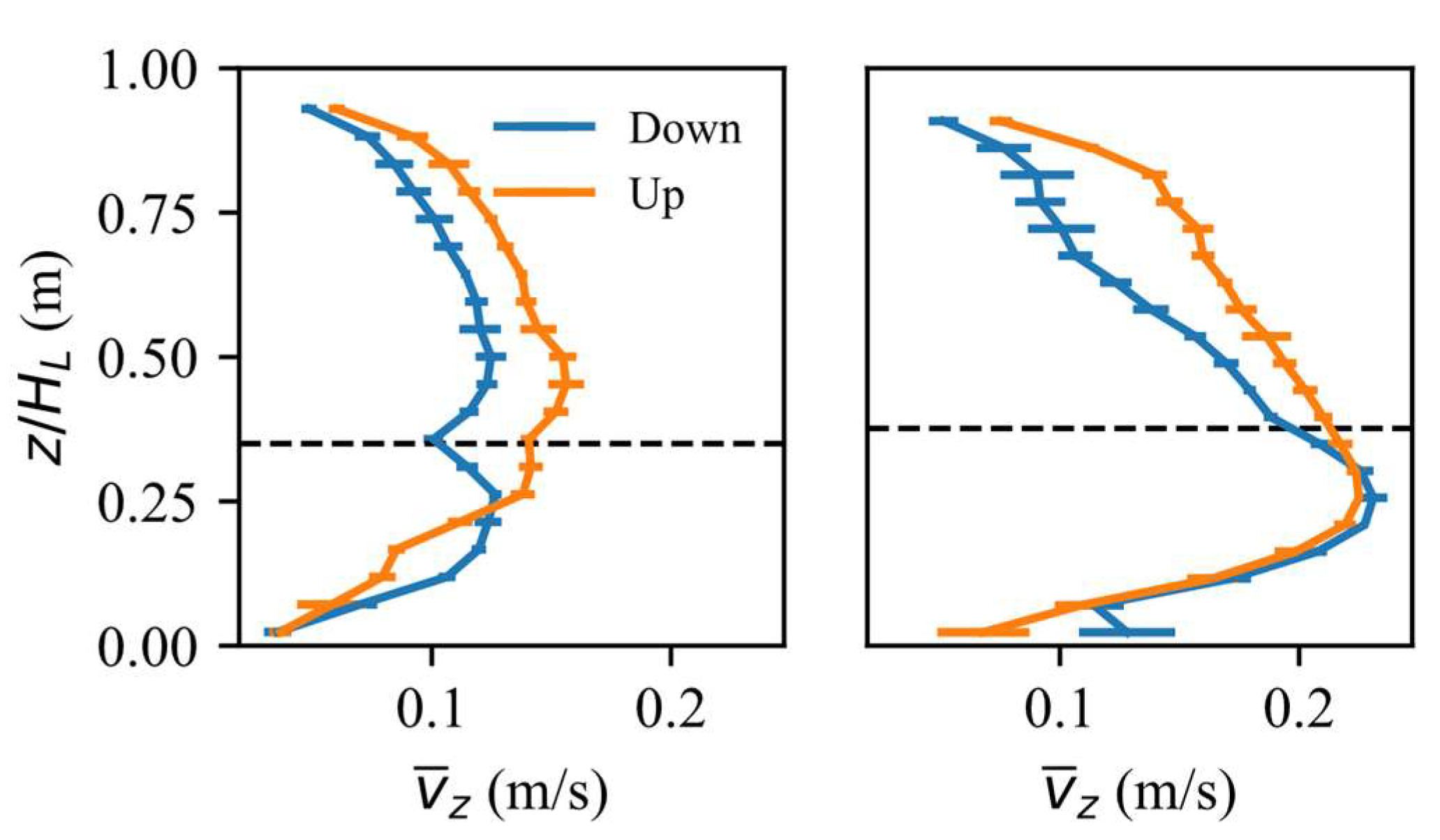
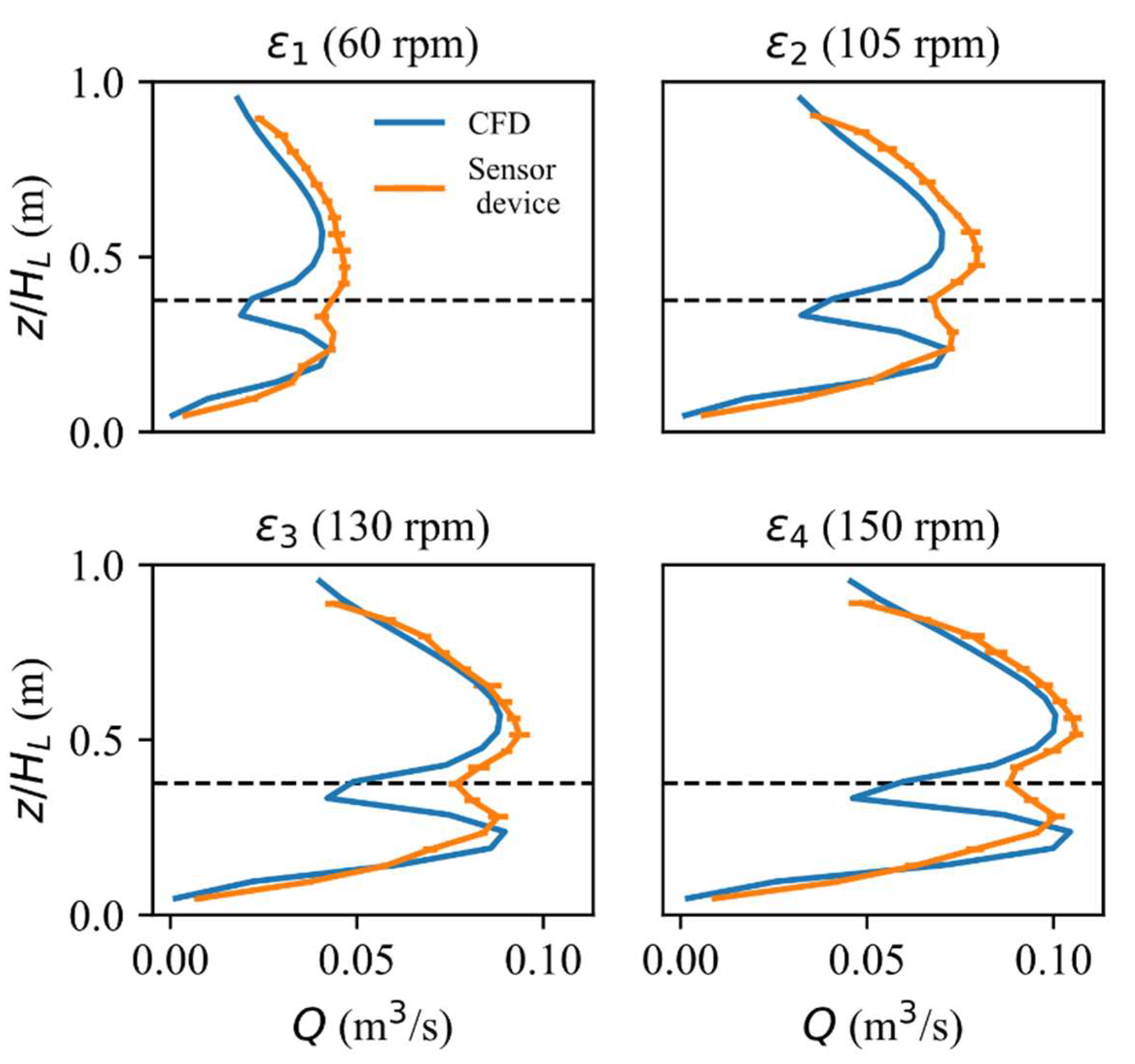
4.1. Comparison of CFD and Sensor Device Derived Flow Rates

The results obtained by the sensor devices have been compared against CFD simulations, which in the case of single-phase flow with the standard k-ε turbulence is believed to satisfactorily represent the true liquid flow. In order to ensure mass conservation in the model, the flows obtained from the average linear velocities in the upwards and downwards direction must be balanced by multiplication with the corresponding areas, according to Equation (4). An example of the average linear velocities in the upwards and the downwards direction as measured by the sensor devices is shown in Figure 3 for the RDT and PBT at ε = ε₁.

Above the impeller, the measured velocities are higher in the upwards direction as compared with the downwards direction, while the velocities are similar, or the opposite is true below the impellers. This means that the areas of the planar compartment interfaces are correspondingly smaller in the upwards flow above the impeller, while they are similar or larger in the flow below the impellers. This situation matches with the flow field over a vertical plane obtained from the CFD simulations, as shown in Figure 4. Here, it is clear that above the impellers the downwards facing velocity vectors constitute a larger cross-sectional area than the velocity vectors facing upwards and therefore higher velocities in the upward flow stream are expected.

A comparison of the flow rates between the compartments obtained by the sensor devices and by CFD for the four different impeller speeds is shown for the RDT in Figure 5. The flow rates obtained by the two approaches are in close agreement. However, close to boundaries, such as the liquid surface, the bottom of the vessel or the impeller, greater deviations exist. At the center of the RDT blade where the liquid flow is pumped directly towards the vessel wall the flow is expected to be primarily radial, and the axial velocity component is expected to be low. The sensor devices do, in some cases, impact with the impeller blade, which suddenly pushes them in different directions. The smaller deviations at the top, bottom and near the impeller could generally be explained by momentum related limitations in the flow following behavior of the flow-following sensor devices due to their considerable diameter. The affected volumes often include crucial interface locations of the compartment model, such as the impeller location, which therefore may introduce considerable errors in the model predictions. The experimental conditions in this study were chosen such that entrainment of air from the liquid surface and cavitation formation behind the impeller blades was negligible. If a significant amount of air is present in the vessel, the compartment volumes and the cross-sectional areas used to calculate the flow rates of the model, should be corrected by an estimate of the liquid fraction. More general challenges related to flow-following behavior and measurement accuracy when using flow-following sensor devices in multi-phase systems have been addressed in [19]. It should also be noted that the standard deviations between the flow rates measured by the four sensor devices are very small, indicating that the individual sensor devices exhibit almost identical behavior.

The same comparison between sensor device measured flow rates and CFD simulated flow rates is shown for the PBT in Figure 6. The same observations with respect to the boundaries apply to this case. However, even greater deviation is present near the impeller where very high velocities are present. Even at the same impeller speeds the PBT produces higher axial velocities compared to the RDT, because the dispersed flow does not separate into two flow streams with opposite directions at the vessel wall as is the case for radial impellers. Sensor devices with large momentum are therefore not able to respond to the changes in the flow fields with high velocities. More importantly, the probability that the sensor devices pass the predominant axial flow through the impeller region is lowered with increasing impeller rotation speeds. In the instances where the sensor devices do not pass the impeller they will be pushed in a radial direction towards the vessel wall, which explains the lower-than-expected axial-flow rates.

These comparisons suggest that the fundamental procedure for extracting the flow rates is appropriate, however, the sensor device technology faces some limitations under the studied experimental conditions. The limitations under these exact conditions have been assessed in greater detail in a previous study [22], in which the flow-following capabilities were addressed using the Stokes number (St), among other things. The Stokes number is a dimensionless number which is commonly used to evaluate the flow following capabilities of a particle and is defined as the ratio between the momentum response time of the particle and a characteristic time of the examined flow [23]. Flow tracers are generally regarded as suitable when the Stokes number is less than 0.1, which as a rule of thumb results in errors of less than 1.0% [24]. The Stokes numbers for the different agitation levels and impeller types were estimated to be in the range of St = 0.2 to St = 0.7 in the circulation flow, while values of the Stokes numbers in the impeller region were as high as St = 9 for the RDT and St = 36 for the PBT at ε = ε₄. In the zones away from the impeller where the sensor devices are expected to represent the circulation flow with reasonable accuracy, the sensor devices seem to overpredict the flow rates. This may be explained by the fact that the linear average axial velocities of the circulation flow represented by the sensor device trajectories are assumed to be representative of the flow over the entire cross-sectional interfaces, which in reality may have areas with lower velocity flow streams that the sensor devices will be entrained in and therefore not sample from. A comparison between the profiles for the CFD predicted flow rates for the PBT (Figure 6) and the velocity profiles of the upwards and downwards flow (Figure 3, right), indicates that the deviations are mainly present in the upwards flow. This could be explained by a predominant entrainment of the sensor devices in the strong flow at the vessel wall, rather than flow streams with lower velocities in the radial section between the impeller and the vessel wall (Figure 4). The differences could also be related to the zone near the shaft at approximately z/H_L = 0.8 (Figure 4), which appears to have a predominant tangential flow.

While more specialized tools are available for examining flows in lab or pilot scale reactors, such as positron emission particle tracking (PEPT) and computer-aided radioactive particle tracking (CARPT) [19], it should be emphasized that flow following sensor devices are specifically designed for large-scale fermentation processes. Large-scale bioreactors typically have circulation times longer than ten seconds [9,25,26]. Therefore, sensor devices with comparable sizes to the ones used in this study are expected to follow the circulation flow in the large-scale bioreactors with similar or higher accuracy than observed for the low speed RDT experiment performed here (St < 0.2) [9]. It should be mentioned that despite CFD models generally predict reality well in simple systems as the ones examined here, inaccuracies are still present.

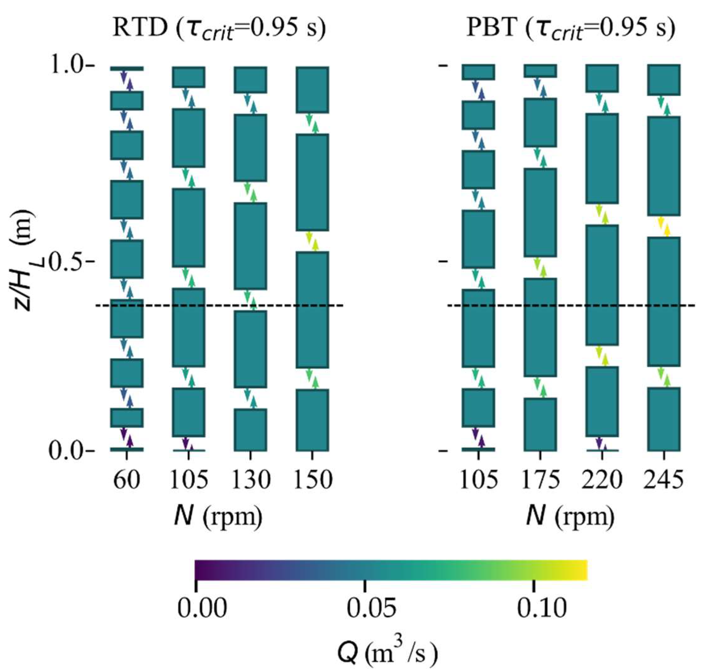
4.2. Comparison of Automatic Zoning

Zoning of compartment models is often performed based on changes in flow pattern, e.g., placing a compartment interface at the impeller in the case of RDTs, which is known to physically compartmentalize and create a barrier for the axial flow [14,27,28]. However, this approach does not account for the situation where the flows inside these compartments are weak and the assumption of perfect mixing fails. Here, the zoning is based on the introduced local residence time in the compartments τ = V/Q, which would further divide such compartments if τ exceeds the threshold τ_crit. τ_crit can also be understood as a relaxation of the condition about perfectly mixed zones, as such zones do not truly exist at this scale. An appropriate value for the critical residence time was found according to the procedure described in Section 3.1.2 to be τ_crit = 0.95 s. The value seems reasonable for the assumption of perfect mixing to be appropriate, i.e., the volume in a compartment should be completely exchanged by the flow from adjacent compartments in approximately one second. It should be mentioned that this value of τ_crit is fitted to the flow rates obtained by the sensor devices, which are known to have errors originating from their flow-following capabilities. Ideally, τ_crit should be obtained by fitting the data from a larger vessel, where these errors are expected to be small. The compartment models which were automatically generated based on the flow rates obtained by the flow-following sensor devices are presented for the RDT and the PBT on the right-hand side and left-hand side of Figure 7, respectively.

For the developed compartment models of all the experimental conditions (Figure 7), the initial compartments in zones with high flow rates expand and decrease in numbers with increasing impeller speeds, which is also what is expected as increasingly larger volumes can be assumed to be perfectly mixed. For the compartment models of the RDT, an interface is placed near the impeller location, with the case of the highest impeller speed being an exception. This agrees with the expected axial-flow barrier generated by the radial flow from the RDT. The interface is not present at the highest impeller speed because the sensor devices measure higher axial-flow rates in this zone than what is expected for the liquid flow, which is evident by the CFD comparison in Figure 5. For the PBT, a compartment for the main circulation flow is expected around and below the impeller. Such a compartment is present for condition ε₁ (105 rpm) and ε₂ (175 rpm), but not for the higher impeller speeds at ε₃ (220 rpm) and ε₄ (245 rpm). This is a result of the higher flow rates measured by the sensor devices above the impeller compared to liquid flow, as discussed in Section 4.1. Towards the top and bottom of the vessel, the flow rates decrease, and an increasing fraction of the velocity component becomes radial. The lower axial exchanges in these zones result in the presence of more compartments, depending on the magnitude of the flow rates.

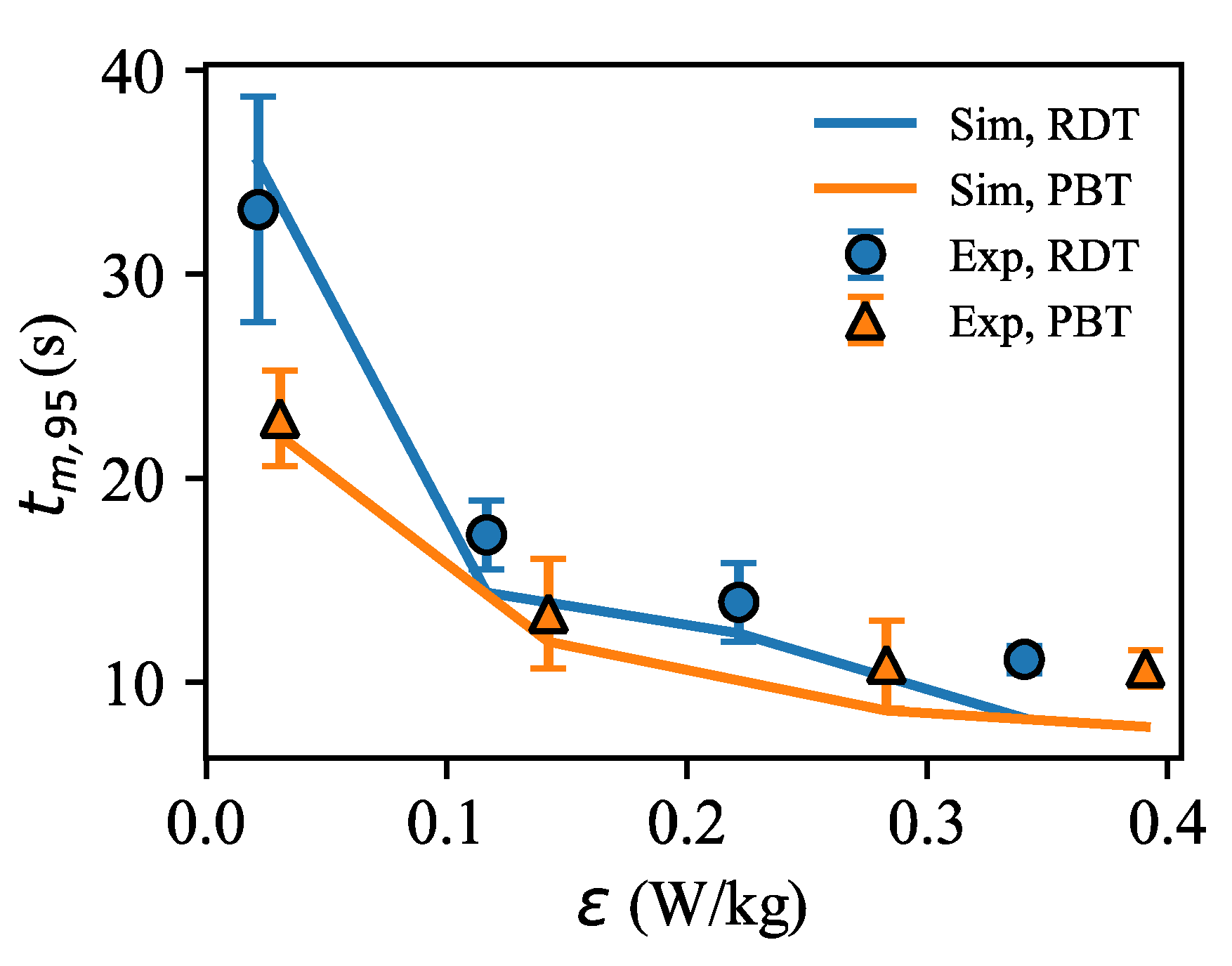
4.3. Comparison of CM-Simulated and Measured Mixing Times

A comparison between the CM-simulated and experimentally determined mixing times for both impeller types is presented in Figure 8.

The CM-simulated mixing times agree well with the measured mixing times, indicating that the model can describe all the examined conditions using a single value for the parameter τ_crit. A quantitative comparison of the relative errors between the CM-simulated mixing times and the experimentally determined mixing times is presented in

Table 1. The relative error between the measured and simulated mixing times, as defined by (t_m,sim-t_m,exp)/t_m,exp for the four examined levels of specific power input (ε₁, ε₂, ε₃, ε₄).

	Relative Error
	ε1	ε2	ε3	ε4
RDT	7% (2.3 s)	−16% (2.8 s)	−11% (1.5 s)	−26% (2.9 s)
PBT	−3% (0.9 s)	−10% (1.4 s)	−21% (2.3 s)	−27% (2.9 s)

.

With the exception of the specific power input ε₂ with the RDT, the relative error increases with increasing impeller speeds at the higher specific power inputs. This trend, including the higher relative error with the RDT at ε₂, matches well with what is expected from the flow rate deviations of the CFD comparisons in Figure 5 and Figure 6, and the discussion in Section 4.1. Despite the large differences between the sensor device measured flow rates and the flow rates from the CFD predictions for the PBT, the errors remain comparable to the errors obtained for the RDT. The reasonable fit for the PBT can be explained by the fact that the zone where major differences between the measured and CFD predicted flow rates exist, was considered perfectly mixed when applying the automatic zoning criteria due to the high axial-flow rates. Therefore, no interfaces were placed in this zone, but instead an interface was placed higher in the vessel where the flow rates are comparable. On the other hand, the lack of interface at the impeller at ε₄ for the RDT likely explains the increased error. A close agreement is observed between the measured mixing times and the mixing times predicted by the models with many axial compartments (at lower levels of specific power inputs). This finding suggests that the commonly used approach to zoning for RDTs, which separates the flow only by the radial flow at the impeller, would significantly underpredict the mixing time.

The sum of squared errors (SSE) between the measured and simulated mixing times for the optimal value of τ_crit was SSE = 14. It should be investigated if this value for τ_crit is more generally applicable for turbulent flow in agitated vessels, or if it is system-specific. It could be imagined that the assumption of perfect radial mixing in the compartments implies a dependency of τ_crit on the interplay between axial- and radial-flow dynamics in the vessel. Following that reasoning, the model predictions will likely improve when the height to diameter ratio of the vessel increases, and the axial mixing becomes the bottleneck.

5. Conclusions

A method for developing compartment models based on data collected by flow-following sensor devices was presented, comprising of two steps. First, derivation of axial-flow rates between a set of initial compartments, and secondly automatic zoning of the vessel volume into a set of axial compartments which can be considered as being perfectly mixed.

It was found that:

• The approach to derive axial-flow rates from the sensor devices was appropriate, however, inaccuracies were present since the sensor devices were not ideal flow tracers.
• A value for the model parameter τ_crit of 0.95 seconds was found to provide the most accurate predictions of the mixing in the vessel for the examined conditions (relative errors between 3–27%).

It is argued here that a value of the parameter τ_crit of approximately one second is reasonable and may be more generally applicable, considering the definition of the zoning criterion “a compartment can from a modelling perspective be assumed to be perfectly mixed if the volume in the compartment is exchanged by the flow from the adjacent compartments in less than a second”. However, this value should be validated for different bioreactor configurations at larger scales by following the same approach as presented in this study.

The method enables the development of flow models that are independent of the experience of the modeler, as all the required information is contained within the collected data. Adaptation of the proposed method to various bioreactor configurations and scales should be straightforward, with little experimental effort required. The flow models can be used to provide potential optimizations for industrial bioprocesses facing problems with mixing and concentration gradients. Such an optimization could be the selection of the optimal location for substrate addition to a process, by minimizing the mixing time with respect to the axial height of the substrate inlet, i.e., compartment. Compartment models can also relatively easily be coupled with models for reaction kinetics and mass transfer to simulate the course of entire fermentation processes, which is not feasible for CFD due to the extensive computation time required for CFD calculations.

References

1. Gernaey, K.V.; Lantz, A.E.; Tufvesson, P.; Woodley, J.M.; Sin, G. Application of mechanistic models to fermentation and biocatalysis for next-generation processes. Trends Biotechnol. 2010, 28, 346–354. [Google Scholar] [CrossRef] [PubMed]
2. Lara, A.R.; Galindo, E.; Ramírez, O.T.; Palomares, L.A. Living with heterogeneities in bioreactors: Understanding the effects of environmental gradients on cells. Mol. Biotechnol. 2006, 34, 355–381. [Google Scholar] [CrossRef]
3. Pigou, M.; Morchain, J.; Fede, P.; Penet, M.I.; Laronze, G. An assessment of methods of moments for the simulation of population dynamics in large-scale bioreactors. Chem. Eng. Sci. 2017, 171, 218–232. [Google Scholar] [CrossRef] [Green Version]
4. Vrábel, P.; Van Der Lans, R.G.J.M.; Luyben, K.C.A.M.; Boon, L.; Nienow, A.W. Mixing in large-scale vessels stirred with multiple radial or radial and axial up-pumping impellers: Modelling and measurements. Chem. Eng. Sci. 2000, 55, 5881–5896. [Google Scholar] [CrossRef]
5. Marshall, E.M.; Bakker, A. Computational Fluid Mixing. In Handbook of Industrial Mixing; John Wiley & Sons: Hoboken, NJ, USA, 2004; pp. 257–343. ISBN 9781444312928. [Google Scholar]
6. Delafosse, A.; Collignon, M.L.; Calvo, S.; Delvigne, F.; Crine, M.; Thonart, P.; Toye, D. CFD-based compartment model for description of mixing in bioreactors. Chem. Eng. Sci. 2014, 106, 76–85. [Google Scholar] [CrossRef]
7. Haringa, C.; Tang, W.; Deshmukh, A.T.; Xia, J.; Reuss, M.; Heijnen, J.J.; Mudde, R.F.; Noorman, H.J. Euler-Lagrange computational fluid dynamics for (bio)reactor scale down: An analysis of organism lifelines. Eng. Life Sci. 2016, 16, 652–663. [Google Scholar] [CrossRef] [PubMed] [Green Version]
8. Vrábel, P.; Van Der Lans, R.G.J.M.; Cui, Y.Q.; Luyben, K.C.A.M. Compartment model approach: Mixing in large scale aerated reactors with multiple impellers. Chem. Eng. Res. Des. 1999, 77, 291–302. [Google Scholar] [CrossRef]
9. Reinecke, S.; Deutschmann, A.; Jobst, K.; Kryk, H.; Friedrich, E.; Hampel, U. Flow following sensor particles-Validation and macro-mixing analysis in a stirred fermentation vessel with a highly viscous substrate. Biochem. Eng. J. 2012, 69, 159–171. [Google Scholar] [CrossRef]
10. Tajsoleiman, T.; Spann, R.; Bach, C.; Gernaey, K.V.; Huusom, J.K.; Krühne, U. A CFD based automatic method for compartment model development. Comput. Chem. Eng. 2019, 123, 236–245. [Google Scholar] [CrossRef]
11. Groen, D.J. Macromixing in Bioreactors; Delft University of Technology: Delft, The Netherlands, 1994. [Google Scholar]
12. Zahradník, J.; Mann, R.; Fialová, M.; Vlaev, D.; Vlaev, S.D.; Lossev, V.; Seichter, P. A networks-of-zones analysis of mixing and mass transfer in three industrial bioreactors. Chem. Eng. Sci. 2001, 56, 485–492. [Google Scholar] [CrossRef]
13. Cui, Y.Q.; Van Der Lans, R.G.J.M.; Noorman, H.J.; Luyben, K.C.A.M. Compartment mixing model for stirred reactors with multiple impellers. Chem. Eng. Res. Des. 1996, 74, 261–271. [Google Scholar]
14. Nørregaard, A.; Bach, C.; Krühne, U.; Borgbjerg, U.; Gernaey, K.V. Hypothesis-driven compartment model for stirred bioreactors utilizing computational fluid dynamics and multiple pH sensors. Chem. Eng. J. 2019, 356, 161–169. [Google Scholar] [CrossRef]
15. Bezzo, F.; Macchietto, S. A general methodology for hybrid multizonal/CFD models: Part II. Automatic zoning. Comput. Chem. Eng. 2004, 28, 513–525. [Google Scholar] [CrossRef]
16. Poulsen, B.R.; Iversen, J.J.L. Mixing determinations in reactor vessels using linear buffers. Chem. Eng. Sci. 1997, 52, 979–984. [Google Scholar] [CrossRef]
17. Brown, D.A.R.; Jones, P.N.; Middelton, J.C. Experimental Methods—Part A: Measuring Tools and Techniques for Mixing and Flow Visualization Studies; John Wiley & Sons: Hoboken, NJ, USA, 2004; ISBN 0-471-26919-0. [Google Scholar]
18. Freesense ApS Fermentation Modelling, Accelerated. Available online: www.freesense.dk/technology (accessed on 23 June 2021).
19. Bisgaard, J.; Muldbak, M.; Cornelissen, S.; Tajsoleiman, T.; Huusom, J.K.; Rasmussen, T.; Gernaey, K.V. Flow-following sensor devices: A tool for bridging data and model predictions in large-scale fermentations. J. Comput. Struct. Biotechnol. 2020, 18, 2908–2919. [Google Scholar] [CrossRef]
20. Enfors, S.O. Continuous and fed-batch fermentation. In Biochemical Engineering Principles; Beroviĉ, M., Nienow, A.W., Eds.; Faculty of Chemistry and Chemical Technology, University of Ljubljana: Ljubljana, Slovenia, 2005; pp. 146–170. [Google Scholar]
21. Bach, C.; Yang, J.; Larsson, H.; Stocks, S.M.; Gernaey, K.V.; Albaek, M.O.; Krühne, U. Evaluation of mixing and mass transfer in a stirred pilot scale bioreactor utilizing CFD. Chem. Eng. Sci. 2017, 171, 19–26. [Google Scholar] [CrossRef]
22. Bisgaard, J.; Muldbak, M.; Tajsoleiman, T.; Rydal, T.; Rasmussen, T.; Huusom, J.K.; Gernaey, K.V. Characterization of mixing performance in bioreactors using flow-following sensor devices. Chem. Eng. Res. Des. 2021. [Google Scholar] [CrossRef]
23. Crowe, C.T.; Schwarzkopf, J.D.; Sommerfeld, M.; Tsuji, Y. Properties of dispersed phase flows. In Multiphase Flows with Droplets and Particles; CRC Press: Boca Raton, FL, USA, 2012; pp. 24–26. [Google Scholar]
24. Tropea, C.; Yarin, A.L.; Foss, J.F. Particle-based techniques. In Handbook of Experimental Fluid Mechanics; Springer: Berlin/Heidelberg, Germany, 2007; pp. 287–290. [Google Scholar]
25. Haringa, C.; Tang, W.; Wang, G.; Deshmukh, A.T.; van Winden, W.A.; Chu, J.; van Gulik, W.M.; Heijnen, J.J.; Mudde, R.F.; Noorman, H.J. Computational fluid dynamics simulation of an industrial P. chrysogenum fermentation with a coupled 9-pool metabolic model: Towards rational scale-down and design optimization. Chem. Eng. Sci. 2018, 175, 12–24. [Google Scholar] [CrossRef]
26. van Barneveld, J.; Smit, W.; Oosterhuis, N.M.G.; Pragt, H.J. Measuring the Liquid Circulation Time in a Large Gas—Liquid Contactor by Means of a Radio Pill. 2. Circulation Time Distribution. Ind. Eng. Chem. Res. 1987, 26, 2192–2195. [Google Scholar] [CrossRef]
27. Spann, R.; Gernaey, K.V.; Sin, G. A compartment model for risk-based monitoring of lactic acid bacteria cultivations. Biochem. Eng. J. 2019, 151, 107293. [Google Scholar] [CrossRef]
28. Amanullah, A.; Buckland, B.C.; Nienow, A.W. Mixing in the Fermentation and Cell Culture Industries. In Handbook of Industrial Mixing; John Wiley & Sons: Hoboken, NJ, USA, 2004; pp. 1071–1170. ISBN 0471269190. [Google Scholar]
Figure 1. Illustration of the stirred vessel used in the study with annotations of important dimensions, locations of sensors and location of the injection point. Left: side view. Right: top view. HL: Liquid height. T: Tank diameter. D: Impeller diameter. C: Impeller clearance. b: Impeller blade height. B: Baffle width. IP: Tracer injection point. S(1–4): Mounted pH sensors.
Processes 09 01651 g001
Figure 2. Schematic representation of the compartment model with K compartments. Mass is exchanged between the ideally mixed volumes (Vk) with the given flow rates (Qk).
Processes 09 01651 g002
Figure 3. Comparison of upwards and downwards velocities measured by the flow-following sensor devices with at ε = ε1, for RDT (left) and PBT (right). The impeller location is represented by the dashed line. The error bars indicate the standard deviation between the measurements of the four sensor devices.
Processes 09 01651 g003
Figure 4. Example of CFD-simulated velocity fields of the stirred vessel at ε = ε1. The left-hand side of the figure shows the velocity fields generated by the RDT, while the right-hand side shows the velocity fields generated by the PBT.
Processes 09 01651 g004
Figure 5. Comparison of flow rates between compartments obtained by CFD (blue) and by the flow-following sensor devices (orange) for the four examined levels of specific power input (ε1, ε2, ε3, ε4) with the RDT. The dashed line represents the impeller location. The error bars indicate the standard deviation between the measurements of the four flow-following sensor devices.
Processes 09 01651 g005
Figure 6. Comparison of flow rates between compartments obtained by CFD (blue) and by the flow-following sensor devices (orange) for the four examined levels of specific power input (ε1, ε2, ε3, ε4) with the PBT. The dashed line represents the impeller location. The error bars indicate the standard deviation between the measurements of the four flow-following sensor devices.
Processes 09 01651 g006
Figure 7. Automatically generated compartment models for the four impeller speeds using the RDT (left) and the PBT (right). The relative heights of the compartments are presented in the y-axis, while the colored arrows between the compartments represent the inter-compartmental flow rates as represented by the color bar. The impeller location is indicated by the dashed line.
Processes 09 01651 g007
Figure 8. Simulated (Sim) and experimentally determined (Exp) mixing times as a function of the specific power input (ε) for the two impeller types (RDT, PBT). The lines depict simulated results for the RDT (blue) and the PBT (orange). The experimental mixing times is presented as circles for the RDT (blue) and triangles for the PBT (orange).
Processes 09 01651 g008