Set Membership Estimation with Dynamic Flux Balance Models

Abstract

Dynamic flux balance models (DFBM) are used in this study to infer metabolite concentrations that are difficult to measure online. The concentrations are estimated based on few available measurements. To account for uncertainty in initial conditions the DFBM is converted into a variable structure system based on a multiparametric linear programming (mpLP) where different regions of the state space are described by correspondingly different state space models. Using this variable structure system, a special set membership-based estimation approach is proposed to estimate unmeasured concentrations from few available measurements. For unobservable concentrations, upper and lower bounds are estimated. The proposed set membership estimation was applied to batch fermentation of E. coli based on DFBM.

1. Introduction

The increasing demand of bio-pharmaceutical products requires continuous improvement in monitoring and control strategies for the fermentation processes. Model-based control and optimization strategies are crucial to boost productivity. Unlike traditional unstructured biochemical models, dynamic flux balance models (DFBM) have gained increasing attention since they contain more detailed information about the distribution of metabolic fluxes [1,2]. The strength of DFBM relies on their use of stoichiometric information about the cell metabolic network. The use of this information often results in models that require a smaller number of parameters as compared to another type of modelling approaches and thus are less prone to over-fitting. However, regardless of the choice of model, monitoring and control of industrial fermentation processes remains challenging because feedback control strategies require many states to be measured online. In reality, most states cannot be measured online either due to the expense of measuring equipment and its maintenance or the lack of online measurement devices [3,4,5]. Some states, including concentration of amino acids, metals, vitamins, ATP and precursors have great effect on the fermentation process but are either difficult or impossible to measure online.

To address the lack of online measurements, soft sensors have been proposed. Soft sensors are algorithms that estimate the values of the states based on few available online measurements. Data-driven soft sensors are currently very popular, driven by the interest in the artificial intelligence research area. Reported data-driven soft sensors are generally based on artificial neural networks, support vector machines, partial least squares, and fuzzy inference [4]. However, despite their popularity, the main drawback of data-driven soft sensors is their limited applicability to the region of data used for model training and the scarcity of data available for calibration [6]. Moreover, the lack of mechanistic information of these black box models introduces concerns about the safety and reliability of the controllers designed based on these models [6].

Another category of soft sensors are state observers based on mechanistic models such as a Luenberger observer, Kalman filter, and particle filter. These state observers estimate the values of some states based on convergence of state prediction errors and provided that sufficient measurements are available [7]. A key prerequisite of theses state observer designs is that some observability condition is satisfied with respect to the estimated states. It will be shown later in the manuscript that, unless enough states of a DFBM model are measured online, it is difficult to satisfy full observability for all the states.

In the absence of observability of some states, instead of estimating their specific values it is possible to estimate intervals (ranges) of values based on a priori known range of initial conditions, i.e., range of values at $\mathrm{time}=0$. This type of problem is referred to in the literature as an initial values problem with parameter uncertainty or set-valued ODE integration. The parameter here refers to either uncertain initial states or some model parameter such as a kinetic constant. In the past several decades, different methods have been proposed to find tight bounds containing the reachable sets, including interval analysis [8], Taylor models with different remainder bounds [9], set-base parameter estimation [10], and different relaxation methods [11]. Due to the uncertainty amplification effect, interval analysis can diverge quickly and only suits a small part of the system. Set-based parameter estimation is computationally expensive because the parameter space need to be validated in a piecewise manner and each validation test requires the solution of a semi-definite programming problem. Taylor models can be used to find tight and nonconvex bounds of reachable sets but cannot be easily formulated to take measurements into consideration. To find the reachable sets compatible with available measurements, different relaxation methods and domain reduction are required which are computationally expensive.

When measurements are available, the trajectories that are not compatible with those measurements should be removed from the reachable sets. Estimation algorithms that efficiently deal with reachable sets subject to measurements including interval observers and set membership estimation algorithms [12,13]. An interval observer is usually composed of two classical observers (framers) which estimate the lower and upper bounds of states, respectively. However, sufficient measurements and fulfillment of observability are still required to build the two classical observers [14,15]. Most interval observers exploit the order-preserving properties of cooperative systems to estimate bounds of states [16]. Set membership estimation is an alternative method for estimating the uncertainty of a set of states that has been applied to linear systems [17]. The propagation of uncertainty along time is performed by a series of affine mapping operations over sets. Different shapes of sets have been used to contain the uncertainty, including zonotopes [18], parallelotopes [17] and ellipsoids [19].

In this research, a set membership estimation approach is proposed for nonlinear systems described by DFBM models. The DFBM is converted into a variable structure system composed of several continuous systems in different region of state space by multiparametric linear programming. To address the lack of measurements an Extended Kalman Filter (EKF) is used to estimate nominal values of some states which are important for determining metabolic fluxes. Then, a set membership estimation algorithm is applied for DFBM to estimate bounds of all states. A detector is proposed to detect the switch between different subsystems.

The paper is organized as follows. Section 2.1 introduces background of DFBM. Section 2.2 describes the use of multiparametric linear programming to convert the DFBM into a variable structure system composed of subsystems. Section 2.3 describes the EKF used to estimate some states which are important for determining metabolic fluxes. Section 2.4 presents the main ideas of set propagation and error compensation for calculation of states’ bounds. Section 2.5 presents the algorithm for detecting the switch between different subsystems. Section 3 provides the application of the proposed techniques to the batch fermentation of E. coli. Section 4 presents a Discussion of the results followed by Conclusions.

2. Materials and Methods

2.1. Dynamic Flux Balance Models

Dynamic flux balance models (DFBM) are structured genome-based metabolic models developed from flux balance models. The key assumption of DFBM is that the cells act as agents distributing resources through metabolic reaction networks to boost a biological objective, e.g., growth rate [1]. Accordingly, the DFBM is formulated as an optimization problem. In the literature [20], both dynamic and static optimization approaches are reported. In the dynamic approach, the nonlinear programming problem is solved over a relatively large time period which is computationally expensive and thus less convenient for uncertainty propagation. In this investigation, static optimization approach is adopted for its simplicity. DFBM is interpreted as a local linear programming problem to maximize a biological objective. In terms of dynamics of intracellular metabolites, there are two type of DFBM models in the literature. One type of DFBM differentiates intracellular and extracellular environments and assumes that the intracellular metabolic reactions are fast enough such as it can be assumed at quasi-steady state [2,21]. Accordingly, only the extracellular metabolites and the biomass are described by dynamic state equations. It has been argued that the intracellular metabolite concentrations are not constant and may change over time [22]. Accordingly, there is a second type of DFBM, used in the current study, which does not differentiate between intracellular and extracellular compartments and the dynamics of all the metabolites are considered [20,23]. The governing equations of DFBM are based on discretized mass balances for all metabolites and these are defined by Equations (1a)–(1d).

$$\begin{array}{cc}\hfill {\mathit{x}}_{\mathit{k}+\mathbf{1}}& =\mathit{B}{\mathit{x}}_{\mathit{k}}+\Delta t{x}_{bio,k}{\mathit{A}\mathit{v}}_{\mathit{k}}+\mathit{h}\hfill \end{array}$$

(1a)

$$\begin{array}{cc}\hfill {\mathit{y}}_{\mathit{k}}& ={\mathit{Cx}}_{\mathit{k}}+{\mathit{r}}_{\mathit{k}}\hfill \end{array}$$

(1b)

$$\begin{array}{cc}\hfill {\mathit{x}}_{\mathbf{0}}& \in {\mathcal{P}}_0\hfill \end{array}$$

(1c)

$$\begin{array}{cc}\hfill {\mathit{r}}_{\mathit{k}}& \sim TN(\mathbf{0},\mathbf{\Sigma },\mathit{l},\mathit{u})k=0,1,2\cdots \hfill \end{array}$$

(1d)

where ${\mathit{x}}_{\mathit{k}}$ is a vector of $n_x$ state variables at the time step k. The state vector $\mathit{x}$ includes concentrations of metabolites and biomass $x_{bio}$. $\mathit{y}$ is a vector of $n_y$ measured variables. $\mathit{B}\in {\mathbb{R}}^{n_x}\times {\mathbb{R}}^{n_x}$ is a constant diagonal matrix with diagonal elements $b_j$, $j=1,\cdots ,n_x$. $\Delta t$ is a constant discrete time step size. $\mathit{A}\in {\mathbb{R}}^{n_x}\times {\mathbb{R}}^{n_{rct}}$ is a stoichiometry coefficient matrix, where $n_{rct}$ is the number of reactions considered in the metabolic network. $\mathit{v}\in {\mathbb{R}}^{n_{rct}}$ is the metabolic flux vector and its calculation is discussed below. $\mathit{h}\in {\mathbb{R}}^{n_x}$ is a constant vector. The initial state ${\mathit{x}}_{\mathbf{0}}$ is assumed to be bounded by a finite polyhedron ${\mathcal{P}}_0$ as Equation (1c). The underlying assumption is that in practice the initial concentrations of the culture medium components are known to be within specific ranges of values ${\mathcal{P}}_0$. This assumption is based on the fact that some variation in media formulation occurs due to human factor and variability in raw materials. Hence, this research focuses on the initial uncertainty and we assume all parameters in the state equations to be known accurately. In other words, the method proposed in this research cannot deal with model structure uncertainty like uncertainty in matrix A. However, the method can be extended to deal indirectly with uncertainty in parameters $\mathit{\theta }$ defined in the following paragraphs.

${\mathit{r}}_{\mathit{k}}\in {\mathbb{R}}^{n_y}$ are measurement noise vectors of which the elements follow the truncated multivariate normal distribution (TN) [24,25]. The probability density function p for $TN(\mathit{\mu },\mathbf{\Sigma },\mathit{l},\mathit{u})$ are defined as per Equation (2).

$$p(\mathit{x},\mathit{\mu },\mathbf{\Sigma },\mathit{l},\mathit{u})=\frac{exp\{-\frac{1}{2}{(\mathit{x}-\mathit{\mu })}^T{\Sigma }^{-1}(\mathit{x}-\mathit{\mu })\}}{{\int }_{\mathit{l}}^{\mathit{u}}exp\{-\frac{1}{2}{(\mathit{x}-\mathit{\mu })}^T{\Sigma }^{-1}(\mathit{x}-\mathit{\mu })\}}$$

(2)

For ${\mathit{r}}_{\mathit{k}}$, the mean vector of TN is $\mathbf{0}\in {\mathbb{R}}^{n_y}$; the covariance is $\mathbf{\Sigma }\in {\mathbb{R}}^{n_y}\times {\mathbb{R}}^{n_y}$; the corresponding variance vector is ${\mathit{\sigma }}^2\in {\mathbb{R}}^{n_y}$; the lower bound and upper bound are $\mathit{l}\in {\mathbb{R}}^{n_y}$ and $\mathit{u}\in {\mathbb{R}}^{n_y}$, respectively. $|·|$ indicates the absolute value of a vector. It is assumed that $|\mathit{l}|\le 3\mathit{\sigma }$ and $|\mathit{u}|\le 3\mathit{\sigma }$, which indicate that the absolute values of the lower bound and upper bound, respectively, are within the range of $3\mathit{\sigma }$. For simplicity, the current study assumes the process noise to be zero. Process noise could be included as an additional state but this is beyond the scope of the current work.

Following the assumption that the cell allocates resources optimally, the metabolic flux $\mathit{v}$ vector at each time step is obtained by solving a linear programming (LP) problem, defined by Equations (3a) and (3b).

$$\begin{array}{ccccc}\hfill & \underset{{\mathit{v}}_{\mathit{k}}}{max}\hfill & \hfill & {\mathit{c}}^T{\mathit{v}}_{\mathit{k}}\hfill & \end{array}$$

(3a)

$$\begin{array}{cccc}\hfill & \mathrm{subject}\mathrm{to}\hfill & \hfill & {\mathit{Gv}}_{\mathit{k}}\le \mathit{F}{\mathit{\theta }}_{\mathit{k}}({\mathit{x}}_{\mathit{k}})+\mathit{z}\hfill \end{array}$$

(3b)

where $\mathit{c}\in {\mathbb{R}}^{n_{rct}}$, $\mathit{F}\in {\mathbb{R}}^{n_G}\times {\mathbb{R}}^{n_{\theta }}$, $\mathit{z}\in {\mathbb{R}}^{n_G}$, $\mathit{G}\in {\mathbb{R}}^{n_G}\times {\mathbb{R}}^{n_{rct}}$, $\mathit{\theta }\in \mathbf{\Theta }\subseteq {\mathbb{R}}^{n_{\theta }}$. $n_G$ is the number of linear constraints. The parameter vector $\mathit{\theta }$ is a nonlinear vector-valued function of states $\mathit{x}$. $n_{\theta }$ denotes the number of elements in the parameter vector $\mathit{\theta }$. Usually, each element $\theta$ is only function of two states at most and one of these two states is biomass concentration. $\mathbf{\Theta }$ denotes the parameter space where the optimal solution of the LP resides. Equation (3a) denotes the objective of the LP that cells are optimizing where the most commonly used objective is the biomass production rate, i.e., growth rate. Thus, cells try to maximize growth rate by allocating limited resources. The LHS (left hand-side) in Equation (3b) describes either the rate of change of metabolite concentrations or the change of metabolite concentrations over a discretization time step $\Delta t$. Matrices $\mathit{G}$ are constant matrices containing the information of the stoichiometry of reactions. RHS in Equation (3b) is a function of ${\mathit{x}}_{\mathit{k}}$, denoting the metabolic reaction bounds for each step. The matrix $\mathit{F}$ is a matrix of which the elements are the part of the right hand side of the constraints that are functions of states at the previous time interval. $\mathit{z}$ is a vector containing constant values such as constant uptake rate limits. Therefore, linear constraints of flux $\mathit{v}$ in Equation (3b) are reaction rate limits or bounds on available resources (nutrients). Numerical examples of these matrices and vectors are shown for the E. coli model in the results section.

2.2. Multiparametric Linear Programming for DFBM

2.2.1. Multiparametric Linear Programming

While set -based methods are available for uncertainty propagation for linear state space equations, these methods are not directly applicable to DFBM. The reason is that the fluxes used in the state equations are obtained from an LP and thus the problem is nonlinear due to the nonlinear function $\mathit{\theta }(\mathit{x})$ and the occurrence of different sets of active constraints. To tackle the dependency of the state equations on the LP, the concept of multiparametric linear programming (mpLP) is used to convert the DFBM into a variable structure system which is composed of subsystems. Multiparametric linear programming divides the parameter space ($\mathbf{\Theta }$) into different regions corresponding to different sets of active constraints and generates explicit expressions for calculating optimal solutions ($\mathit{v}$) for each region [26,27,28].

Let assume a given optimal solution $\mathit{v}$ of the LP (Equation (3)) where subscript $\mathcal{A}$ and $\mathcal{I}$ denote indices of active and inactive constraints, respectively. Using this notation Equation (3b) is decomposed into two parts, equalities ${\mathit{G}}_{\mathcal{A}}{\mathit{v}}_{\mathit{k}}={\mathit{F}}_{\mathcal{A}}{\mathit{\theta }}_{\mathit{k}}({\mathit{x}}_{\mathit{k}})+{\mathit{z}}_{\mathcal{A}}$ and inequalities ${\mathit{G}}_{\mathcal{I}}{\mathit{v}}_{\mathit{k}}\le {\mathit{F}}_{\mathcal{I}}{\mathit{\theta }}_{\mathit{k}}({\mathit{x}}_{\mathit{k}})+{\mathit{z}}_{\mathcal{I}}$. Without loss of generality, let us assume that ${\mathit{G}}_{\mathcal{A}}$ is linear independent (linear redundant rows can always been removed by Gaussian elimination). Let $\mathit{H}={\mathit{G}}_{\mathcal{A}}^{-\mathbf{1}}{\mathit{F}}_{\mathcal{A}}$ and $\mathit{g}={\mathit{G}}_{\mathcal{A}}^{-\mathbf{1}}{\mathit{z}}_{\mathcal{A}}$, then the optimal solution can be obtained by Equation (4).

$${\mathit{v}}_{\mathit{k}}=\mathit{H}{\mathit{\theta }}_{\mathit{k}}({\mathit{x}}_{\mathit{k}})+\mathit{g}$$

(4)

Substituting Equation (4) into the inequality constraints results in Equation (5).

$$({\mathit{G}}_{\mathcal{I}}\mathit{H}-{\mathit{F}}_{\mathcal{I}}){\mathit{\theta }}_{\mathit{k}}({\mathit{x}}_{\mathit{k}})<{\mathit{z}}_{\mathcal{I}}-{\mathit{G}}_{\mathcal{I}}\mathit{g}$$

(5)

Equation (5) defines a polyhedral region of $\mathit{\theta }$ where the existence of the optimal solution is ensured by Equation (4). The region defined by Equation (5) is referred to as a critical region in the multiparametric programming literature. Different critical regions are defined by different combinations of $\mathcal{A}$ and $\mathcal{I}$. Then, the entire parameter space $\mathbf{\Theta }$ can be decomposed into connected critical regions denoted by $\{{\mathbf{\Theta }}^i\},i=1,\cdots ,n_{\mathbf{\Theta }}$. $n_{\mathbf{\Theta }}$ denotes the total number of critical regions in $\mathbf{\Theta }$. In practice, critical regions that are very small are ignored and assumed to be covered by the adjacent critical region. Correspondingly, superscript i is used to denotes the i-th critical region. Assume for a specific $\mathit{\theta }\in {\mathbf{\Theta }}^i$, the optimal flux $\mathit{v}$ vector can be calculated analytically by ${\mathit{v}}_{\mathit{k}}^{\mathit{i}}={\mathit{H}}^{\mathit{i}}{\mathit{\theta }}_{\mathit{k}}+{\mathit{g}}^{\mathit{i}}$ thus bypassing the need for solving the LP. Following the literature and our previous studies, for a given $\mathit{\theta }$, multiple optimal solutions can coexist [29,30]. In other words, multiple Equation (4) can coexist which results in different ways to divide the parameter space $\mathbf{\Theta }$. When such multiplicity issue occurs it results in different time trajectories. For simplicity, multiplicity is not addressed in the current study and it is addressed in a separate work by different methods from the one presented here.

By substituting the optimizer equation ${\mathit{v}}_{\mathit{k}}^{\mathit{i}}={\mathit{H}}^{\mathit{i}}{\mathit{\theta }}_{\mathit{k}}+{\mathit{g}}^{\mathit{i}}$ into Equation (1a), we obtained a set of governing state equations as per Equations (6a)–(6e). Since different ${\mathit{\theta }}_{\mathit{k}}$ are within different critical regions as Equation (6b), each critical region corresponds to different state equations Equation (6a). Thus the set $\{{\mathbf{\Theta }}^{\mathit{i}}\}$ defines a family of state space models and this family is referred to as a variable structure system. A variable structure system is a piecewise continuous system composed of subsystems where each subsystem corresponds to a different region of the state space. Furthermore, the region of the state space corresponding to a specific subsystem is referred to as a critical region. Each subsystem is described by a different set of state equations. Accordingly, the state equations need to be changed as soon as the states enter into a new critical region. Here, the superscript i denotes the i-th subsystem corresponding to a critical region ${\mathbf{\Theta }}^{\mathit{i}}$. Equations (6c)–(6e) remain the same form as Equations (1b)–(1d).

$$\begin{array}{cc}\hfill {\mathit{x}}_{\mathit{k}+\mathbf{1}}& =\mathit{B}{\mathit{x}}_{\mathit{k}}+\Delta t{x}_{bio,k}\mathit{A}({\mathit{H}}^{\mathit{i}}{\mathit{\theta }}_{\mathit{k}}({\mathit{x}}_{\mathit{k}})+{\mathit{g}}^{\mathit{i}})+\mathit{h}\hfill \end{array}$$

(6a)

$$\begin{array}{cc}\hfill {\mathit{\theta }}_{\mathit{k}}& ({\mathit{x}}_{\mathit{k}})\in {\mathbf{\Theta }}^{i}i=1,\cdots ,n_{\mathbf{\Theta }}\hfill \end{array}$$

(6b)

$$\begin{array}{cc}\hfill {\mathit{y}}_{\mathit{k}}& ={\mathit{Cx}}_{\mathit{k}}+{\mathit{r}}_{\mathit{k}}\hfill \end{array}$$

(6c)

$$\begin{array}{cc}\hfill {\mathit{x}}_{\mathbf{0}}& \in {\mathcal{P}}_0\hfill \end{array}$$

(6d)

$$\begin{array}{cc}\hfill {\mathit{r}}_{\mathit{k}}& \sim TN(\mathbf{0},\mathbf{\Sigma },\mathit{l},\mathit{u})k=0,1,2\cdots \hfill \end{array}$$

(6e)

2.2.2. Reaction Rate Estimability

To further simplify the system described by Equations (6a)–(6e) it is possible to exploit the sparseness of the $\mathit{H}$ matrix. For instance, to take advantage of zero columns of $\mathit{H}$, Equation (4) can be re-written as shown in Equation (7). For conciseness, the subscript k is omitted here because Equation (7) applies for all time steps.

$${\mathit{v}}^{\mathit{i}}={\mathit{H}}^{\mathit{i}}\mathit{\theta }(\mathit{x})+{\mathit{g}}^{\mathit{i}}=\left[\begin{array}{cc}{\mathit{H}}_{\mathit{N}}^{\mathit{i}}& {\mathit{H}}_{\mathit{Z}}^{\mathit{i}}\end{array}\right]\left[\begin{array}{c}{\mathit{\theta }}_{\mathit{N}}^{\mathit{i}}({\mathit{x}}_{\mathit{N}}^{\mathit{i}})\\ {\mathit{\theta }}_{\mathit{Z}}^{\mathit{i}}(\mathit{x})\end{array}\right]+{\mathit{g}}^{\mathit{i}}={\mathit{H}}_{\mathit{N}}^{\mathit{i}}{\mathit{\theta }}_{\mathit{N}}^{\mathit{i}}({\mathit{x}}_{\mathit{N}}^{\mathit{i}})+{\mathit{g}}^{\mathit{i}}$$

(7)

In Equation (7) N and Z denote the indices of the nonzero and zero columns of the $\mathit{H}$ matrix, respectively. Because ${\mathit{H}}_{\mathit{Z}}$ is a submatrix containing the zero columns of $\mathit{H}$, the flux $\mathit{v}$ is only a function of parameters ${\mathit{\theta }}_{\mathit{N}}({\mathit{x}}_{\mathit{N}})$ according to Equation (7). Moreover, while the parameters $\mathit{\theta }$ are a function of states $\mathit{x}$ (see Equations Equations (1a)–(1d) and (3)), only some elements of $\mathit{x}$ actually determine the entire flux vector $\mathit{v}$. The vector ${\mathit{x}}_{\mathit{N}}$ contains, according to Equation (7), the states that determine the flux vector. Notice that for different critical regions flux-determining vector ${\mathit{x}}_{\mathit{N}}$ contains different states. Therefore, Equation (6a) can be simplified into Equation (8).

$${\mathit{x}}_{\mathit{k}+\mathbf{1}}=\mathit{B}{\mathit{x}}_{\mathit{k}}+\Delta t{x}_{bio,k}\mathit{A}({\mathit{H}}_{\mathit{N}}^{\mathit{i}}{\mathit{\theta }}_{\mathit{N}}^{\mathit{i}}({\mathit{x}}_{\mathit{N},\mathit{k}}^{\mathit{i}})+{\mathit{g}}^{\mathit{i}})+\mathit{h}$$

(8)

The biological interpretation of the flux-determining state vector ${\mathit{x}}_{\mathit{N}}$ is that only some resources are limiting the growth of cells, either because they are limited or because the activity of enzymes in the related reactions (fluxes) is limiting. As the fermentation progresses, the states transit into new critical regions from old critical regions. Different critical regions can be interpreted as different metabolic stages where ${\mathit{x}}_{\mathit{N}}$ are different. Similar interpretations have been reported in [26] in the context of steady state flux balance analysis.

In Equation (8), the term $\Delta t{x}_{bio,k}\mathit{A}({\mathit{H}}_{\mathit{N}}^{\mathit{i}}{\mathit{\theta }}_{\mathit{N}}^{\mathit{i}}({\mathit{x}}_{\mathit{N},\mathit{k}}^{\mathit{i}})$ denotes the change of metabolite concentrations contributed by metabolic reactions. Therefore, the reaction rates are $x_{bio,k}\mathit{A}({\mathit{H}}_{\mathit{N}}^{\mathit{i}}{\mathit{\theta }}_{\mathit{N}}^{\mathit{i}}({\mathit{x}}_{\mathit{N},\mathit{k}}^{\mathit{i}})$. It is noted that this nonlinear reaction rate term is not only a function of the flux-determining states vector ${\mathit{x}}_{\mathit{N}}$ but also of biomass concentration $x_{bio}$, because the fluxes are defined per unit biomass, i.e., more biomass demands more nutrients to satisfy the requirement of the growth. Once the states that determine the reaction rates, i.e., the states ${\mathit{x}}_{\mathit{N}}$ together with the value of $x_{bio}$, can be estimated, the estimation problem can be simplified greatly. Since in some cases ${\mathit{x}}_{\mathit{N}}$ contains $x_{bio}$ but in some cases it does not, we define a reaction-rate-determining state vector ${\mathit{x}}_{\mathit{M}}$ in Equation (9). Hence, the reaction-rate-determining state vector ${\mathit{x}}_{\mathit{M}}$ always contains the flux-determining states ${\mathit{x}}_{\mathit{N}}$ and the biomass state $x_{bio}$ without any redundancy.

$${\mathit{x}}_{\mathit{M}}=\left\{\begin{array}{cc}{\mathit{x}}_{\mathit{N}},\hfill & \mathrm{if}{\mathit{x}}_{\mathit{N}}\mathrm{contains}\mathrm{the}\mathrm{biomass}\mathrm{state}{x}_{bio}.\hfill \\ \left[\begin{array}{c}{\mathit{x}}_{\mathit{N}}\\ x_{bio}\end{array}\right],\hfill & \mathrm{otherwise}.\hfill \end{array}\right.$$

(9)

The vector ${\mathit{x}}_{\mathit{M}}$ for critical region ${\mathbf{\Theta }}^{\mathit{i}}$ is denoted by ${\mathit{x}}_{\mathit{M}}^{\mathit{i}}$. We define reaction rate estimability as the ability to determine the reaction rates $x_{bio,k}\mathit{A}({\mathit{H}}_{\mathit{N}}^{\mathit{i}}{\mathit{\theta }}_{\mathit{N}}^{\mathit{i}}({\mathit{x}}_{\mathit{N},\mathit{k}}^{\mathit{i}})$ in the metabolic networks which is needed for the calculation of Equation (8). Following the above, once reaction-rate-determining state vector ${\mathit{x}}_{\mathit{M}}$ at time step k can be estimated, the dynamic evolution of the culture at step $k+1$ as per Equation (8) can be predicted. In addition, it should be noticed that it is not necessary to measure all the reaction-rate-determining states for reaction rate estimability and instead some states can be estimated by an observer from available measurements. However, if an observer is used to estimate ${\mathit{x}}_{\mathit{M}}^{\mathit{i}}$, some particular combination of measurements is necessary for observability of ${\mathit{x}}_{\mathit{M}}^{\mathit{i}}$. Considering different measurement combinations ${\Omega }_1^i,{\Omega }_2^i...$ for the critical region ${\mathbf{\Theta }}^{\mathit{i}}$, only some combinations provide full observability of ${\mathit{x}}_{\mathit{M}}^{\mathit{i}}$. Let ${\Omega }_{\mathcal{O}}^i$ be defined as a family of sets of measurements, which contains all measurement combinations that fulfill observability of ${\mathit{x}}_{\mathit{M}}^{\mathit{i}}$.

Although many different critical regions and corresponding combinations of measurements could be considered, in practice the possibilities will be limited because industrial fermentations usually operate in a narrow range of operating conditions. Thus, the dynamic trajectories of states only pass through a limited set of critical regions. Assume for $\forall {\mathit{x}}_{\mathbf{0}}\in {\mathcal{P}}_0$, the set of critical regions that the trajectories traverse are $\Gamma$. Then, the minimum set of measurements required for the reaction rate estimability of the critical region set $\Gamma$ is ${\Omega }_{\Gamma }$ as per Equations (10a)–(10c).

$$\begin{array}{ccc}\hfill & {\Omega }_{\Gamma }=\underset{j}{min}|\bigcup _i{\Omega }_j^i|\hfill & \end{array}$$

(10a)

$$\begin{array}{ccc}\hfill & \mathrm{subject}\mathrm{to}i\in \Gamma \hfill & \end{array}$$

(10b)

$$\begin{array}{cc}\hfill & {\Omega }_j^i\in {\Omega }_{\mathcal{O}}^i\hfill \end{array}$$

(10c)

where $|·|$ is the cardinality of a finite countable set, i.e., the number of elements of a set. In Equation (10c), ${\Omega }_j^i\in {\Omega }_{\mathcal{O}}^i$ indicates that the measurement combination ${\Omega }_j^i$ can fulfill the observability of reaction-rate-determining states ${\mathit{x}}_{\mathit{M}}^{\mathit{i}}$ of critical region ${\mathbf{\Theta }}^{\mathit{i}}$. If all states in set ${\Omega }_{\Gamma }$ are measured, the reaction rate term of any trajectory starting from ${\mathcal{P}}_0$ can be estimated by the observer. In other words, although ${\mathit{x}}_{\mathit{M}}^{\mathit{i}}$ in different critical regions may be different, requiring different measurements for observability, ${\mathit{x}}_{\mathit{M}}^{\mathit{i}}$ is always observable if the chosen set of measurements satisfy Equation (10c).

2.3. Extended Kalman Filter (EKF)

Using the minimum required set of measurements, ${\Omega }_{\Gamma }$ is defined in Equation (10c), ${\mathit{x}}_{\mathit{M}}$ can be estimated by an observer. ${\mathit{x}}_{\mathit{M}}$ corresponds to the observable subspace of the governing equation (Equations (1a)–(1d)) for each critical region. The state equation of the observable subspace for critical region ${\mathbf{\Theta }}^{\mathit{i}}$ is given by Equations (11a)–(11c).

$$\begin{array}{cc}\hfill {\mathit{x}}_{\mathit{M},\mathit{k}+\mathbf{1}}^{\mathit{i}}& ={\mathit{f}}^i({\mathit{x}}_{\mathit{M},\mathit{k}}^{\mathit{i}})=\mathit{B}{\mathit{x}}_{\mathit{M},\mathit{k}}^{\mathit{i}}+\Delta t{x}_{bio,k}{\mathit{A}}_{\mathit{M}}({\mathit{H}}_{\mathit{N}}^{\mathit{i}}{\mathit{\theta }}_{\mathit{N}}^{\mathit{i}}({\mathit{x}}_{\mathit{N},\mathit{k}}^{\mathit{i}})+{\mathit{g}}^{\mathit{i}})+{\mathit{h}}_{\mathit{M}}\hfill \end{array}$$

(11a)

$$\begin{array}{cc}\hfill {\mathit{y}}_{\mathit{k}}& ={\mathit{C}}_{\mathit{M}}^{\mathit{i}}{\mathit{x}}_{\mathit{M},\mathit{k}}^{\mathit{i}}+{\mathit{r}}_{\mathit{k}}\hfill \end{array}$$

(11b)

$$\begin{array}{cc}\hfill {\mathit{r}}_{\mathit{k}}& \sim TN(\mathbf{0},\mathbf{\Sigma },\mathit{l},\mathit{u})k=0,1,2\cdots \hfill \end{array}$$

(11c)

where ${\mathit{x}}_{\mathit{N},\mathit{k}}^{\mathit{i}}$ and ${\mathit{x}}_{\mathit{M},\mathit{k}}^{\mathit{i}}$ are the flux-determining state vector and the reaction-rate-determining state vector for critical region ${\mathbf{\Theta }}^{\mathit{i}}$, respectively; ${\mathit{A}}_{\mathit{M}}$ is the stoichiometry submatrix corresponding to ${\mathit{x}}_{\mathit{M}}$. Similarly ${\mathit{h}}_{\mathit{M}}$ is a sub-vector of $\mathit{h}$ corresponding to ${\mathit{x}}_{\mathit{M}}$. It should be noticed that, for different critical regions, ${\mathit{x}}_{\mathit{M}}$ involves different states. Accordingly, each critical region requires the use of a different EKF. In addition, it should be noticed that the ${\mathit{C}}_{\mathit{M}}^{\mathit{i}}$ matrices are different for each critical region but the measured variables ${\Omega }_{\Gamma }$ are the same since the same sensors are used for the entire fermentation.

To estimate ${\mathit{x}}_{\mathit{M}}^{\mathit{i}}$, an standard EKF is used due to its effective and simple structure [31]. The estimate ${\widehat{\mathit{x}}}_{\mathit{M},\mathit{k}}^{\mathit{i}}$ and covariance ${\mathit{P}}_{\mathit{k}}^{\mathit{i}}$ of ${\mathit{x}}_{\mathit{M}}^{\mathit{i}}$ for critical region ${\mathbf{\Theta }}^{\mathit{i}}$ are described by Equation (12a) and Equation (12b), respectively.

$$\begin{array}{cc}\hfill {\widehat{\mathit{x}}}_{\mathit{M},\mathit{k}}^{\mathit{i}}& ={\mathit{f}}^i({\widehat{\mathit{x}}}_{\mathit{M},\mathit{k}-\mathbf{1}}^{\mathit{i}})+{\mathit{K}}_{\mathit{k}}({\mathit{y}}_{\mathit{k}}-{\mathit{C}}_{\mathit{M}}^{\mathit{i}}{\mathit{f}}^{\mathit{i}}({\widehat{\mathit{x}}}_{\mathit{M},\mathit{k}-\mathbf{1}}^{\mathit{i}}))\hfill \end{array}$$

(12a)

$$\begin{array}{cc}\hfill {{\mathit{P}}_{\mathit{k}}^{\mathit{i}}}^{-\mathbf{1}}& ={\mathsf{\Phi }}_{\mathit{k}-\mathbf{1}}^{\mathit{i}}{\mathit{P}}_{\mathit{k}-\mathbf{1}}^{\mathit{i}}{{\mathsf{\Phi }}_{\mathit{k}-\mathbf{1}}^{\mathit{i}}}^T+{{\mathit{C}}_{\mathit{M}}^{\mathit{i}}}^T{({\mathbf{\Sigma }\mathbf{\Sigma }}^T)}^{-1}{\mathit{C}}_{\mathit{M}}^{\mathit{i}}\hfill \end{array}$$

(12b)

where

$$\begin{array}{cc}\hfill {\mathit{K}}_{\mathit{k}}& ={\mathsf{\Phi }}_{\mathit{k}-\mathbf{1}}^{\mathit{i}}{\mathit{P}}_{\mathit{k}-\mathbf{1}}^{\mathit{i}}{{\mathsf{\Phi }}_{\mathit{k}-\mathbf{1}}^{\mathit{i}}}^T{{\mathit{C}}_{\mathit{M}}^{\mathit{i}}}^T{({\mathit{C}}_{\mathit{M}}^{\mathit{i}}{\mathsf{\Phi }}_{\mathit{k}-\mathbf{1}}^{\mathit{i}}{\mathit{P}}_{\mathit{k}-\mathbf{1}}{{\mathsf{\Phi }}_{\mathit{k}-\mathbf{1}}^{\mathit{i}}}^T{{\mathit{C}}_{\mathit{M}}^{\mathit{i}}}^T+{\mathbf{\Sigma }\mathbf{\Sigma }}^T)}^{-1}\hfill \end{array}$$

(13a)

$$\begin{array}{cc}\hfill {\mathsf{\Phi }}_{\mathit{k}}^{\mathit{i}}& =\frac{\partial {\mathit{f}}^i}{\partial {\mathit{x}}_{\mathit{M}}^{\mathit{i}}}({\widehat{\mathit{x}}}_{\mathit{M},\mathit{k}}^{\mathit{i}})\hfill \end{array}$$

(13b)

The measurement noise is assumed to be a truncated multivariate normal distribution as Equation (11c). This assumption is needed for estimating finite bounds as explained in the following section. Recall in Equation (2) that $|\mathit{l}|\le 3\mathit{\sigma }$ and $|\mathit{u}|\le 3\mathit{\sigma }$, the lower and upper bounds are located within the range of $3\mathit{\sigma }$. The covariance matrix ${\mathit{P}}_{\mathit{k}}$ is always overestimated to ensure boundedness. Although the EKF resulting from this assumption is sub-optimal, it is still sufficient to estimate ${\mathit{x}}_{\mathit{M}}^{\mathit{i}}$.

2.4. Set Propagation and Error Compensation

Since the minimum set of measurements defined by Equations (10a)–(10c) can only ensure the observability of ${\mathit{x}}_{\mathit{M}}$, the estimation of other states needs different estimation strategies. The idea is to exploit the a priori knowledge of the initial ranges of initial conditions to estimate all states. Instead of predicting specific values of states, set membership estimation (SME) approach is used to predict sets containing all possible states by a series of set operations. These set operations usually include linear mapping, projection, translation, Minkowski addition, intersection, union, and outer approximation. In this research, all sets and multiparametric linear programming operations are performed with the Multi-Parametric Toolbox 3.0 (https://www.mpt3.org/ accessed on 15 July 2021) [32] and MATLAB R2018a. The E. coli example can be found online (https://github.com/SetMembershipEstimationDFBM/E.coliExample, accessed on 25 September 2021). For DFBM, SME propagates the initial set ${\mathcal{P}}_0$ by affine mapping as Equation (14). Affine mapping involves two operations: linear mapping of the previous set and translation.

$${\widehat{\mathcal{X}}}_{k+1}\approx \underset{\mathrm{linear}\mathrm{mapping}}{\underbrace{\mathit{B}{\widehat{\mathcal{X}}}_k}}+\underset{\mathrm{translation}}{\underbrace{\Delta t{\widehat{x}}_{bio,k}\mathit{A}({\mathit{H}}_{\mathit{N}}^{\mathit{i}}{\mathit{\theta }}_{\mathit{N}}^{\mathit{i}}({\widehat{\mathit{x}}}_{\mathit{N},\mathit{k}}^{\mathit{i}})+{\mathit{g}}^{\mathit{i}})+\mathit{h}}}$$

(14)

where ${\widehat{\mathcal{X}}}_k$ represents the set of states at time step k and ${\widehat{\mathcal{X}}}_0={\mathcal{P}}_0$, i.e., the set of initial conditions assumed to be known. In Equation (14), the translation term is approximated by using the estimate ${\widehat{\mathit{x}}}_{\mathit{M},\mathit{k}}^{\mathit{i}}$ obtained by the EKF. In the application of EKF, the estimate ${\widehat{\mathit{x}}}_{\mathit{M},\mathit{k}}^{\mathit{i}}$ needs several time steps to converge to the true flux-determining states ${\mathit{x}}_{\mathit{M},\mathit{k}}^{\mathit{i}}$. Thus the SME described by Equation (14) may underestimate bounds while the EKF is converging. To mitigate this problem, a correction is implemented to compensate for the estimate error as described below. Since no extra information is available, the compensation of the estimate error is based on the worst case scenario.

The error in the estimate incurred by the observer for critical region ${\mathbf{\Theta }}^{\mathit{i}}$ is ${\mathit{e}}_{\mathit{M}}^{\mathit{i}}={\mathit{x}}_{\mathit{M},\mathit{k}}^{\mathit{i}}-{\widehat{\mathit{x}}}_{\mathit{M},\mathit{k}}^{\mathit{i}}$. Since ${\mathit{x}}_{\mathit{M},\mathit{k}}^{\mathit{i}}$ always contains biomass $x_{bio,k}^i$ and ${\mathit{x}}_{\mathit{N},\mathit{k}}^{\mathit{i}}$, the corresponding estimate errors are defined as ${\mathit{e}}_{\mathit{N},\mathit{k}}^{\mathit{i}}={\mathit{x}}_{\mathit{N},\mathit{k}}^{\mathit{i}}-{\widehat{\mathit{x}}}_{\mathit{N},\mathit{k}}^{\mathit{i}}$ and $e_{bio}^i=x_{bio,k}^i-{\widehat{x}}_{bio,k}^i$. Let us assume that the function $\mathit{\theta }$ is first-order differentiable and define Jacobian matrix ${\mathit{\psi }}_{\mathit{k}}^{\mathit{i}}$.

$${\mathit{\psi }}_{\mathit{k}}^{\mathit{i}}=\frac{\partial {\mathit{\theta }}_{\mathit{N}}^{\mathit{i}}}{\partial {\mathit{x}}_{\mathit{N}}^{\mathit{i}}}({\widehat{\mathit{x}}}_{\mathit{N},\mathit{k}}^{\mathit{i}})$$

(15)

Substituting the estimate error ${\mathit{e}}_{\mathit{k}}^{\mathit{i}}$, $e_{bio}^i$ and Jacobian matrix ${\mathit{\psi }}_{\mathit{k}}^{\mathit{i}}$ into Equation (8), a corrected state equation that accounts for the estimate error is obtained as Equations (16a) and (16b). Equations (16a) and (16b) uses a first order approximation to account for the state deviation ${\mathit{ϵ}}_{\mathit{k}}^{\mathit{i}}$ caused by the estimate error ${\mathit{e}}_{\mathit{M},\mathit{k}}^{\mathit{i}}$, while the EKF is converging. The error compensation based on linearization provides satisfactory bounds because the error between estimate and measured is small and decreases quickly due to the convergence of EKF.

$$\begin{array}{cc}\hfill {\mathit{x}}_{\mathit{k}+\mathbf{1}}& =\mathit{B}{\mathit{x}}_{\mathit{k}}+\Delta t{\widehat{x}}_{bio,k}\mathit{A}({\mathit{H}}_{\mathit{N}}^{\mathit{i}}{\mathit{\psi }}_{\mathit{k}}^{\mathit{i}}{\widehat{\mathit{x}}}_{\mathit{N},\mathit{k}}^{\mathit{i}}+{\mathit{g}}^{\mathit{i}})+\mathit{h}+{\mathit{ϵ}}_{\mathit{k}}^{\mathit{i}}\hfill \end{array}$$

(16a)

$$\begin{array}{cc}\hfill {\mathit{ϵ}}_{\mathit{k}}^{\mathit{i}}& ={\mathit{D}}_{\mathit{k}}{\mathit{e}}_{\mathit{N},\mathit{k}}^{\mathit{i}}+e_{bio,k}{\mathit{M}}_{\mathit{k}}{\mathit{e}}_{\mathit{N},\mathit{k}}^{\mathit{i}}+{\mathit{L}}_{\mathit{k}}{e}_{bio,k}\hfill \end{array}$$

(16b)

where

$$\begin{array}{cc}\hfill {\mathit{D}}_{\mathit{k}}& ={\widehat{x}}_{bio,k}\Delta t{\mathit{AH}}_{\mathit{N}}^{\mathit{i}}{\mathit{\psi }}_{\mathit{k}}^{\mathit{i}}+\mathit{h}\hfill \end{array}$$

(17a)

$$\begin{array}{cc}\hfill {\mathit{M}}_{\mathit{k}}& =\Delta t{\mathit{AH}}_{\mathit{N}}^{\mathit{i}}{\mathit{\psi }}_{\mathit{k}}^{\mathit{i}}\hfill \end{array}$$

(17b)

$$\begin{array}{cc}\hfill {\mathit{L}}_{\mathit{k}}& =\Delta t\mathit{A}({\mathit{H}}_{\mathit{N}}^{\mathit{i}}{\mathit{\theta }}_{\mathit{N},\mathit{k}}^{\mathit{i}}({\widehat{\mathit{x}}}_{\mathit{N},\mathit{k}}^{\mathit{i}})+{\mathit{g}}^{\mathit{i}})\hfill \end{array}$$

(17c)

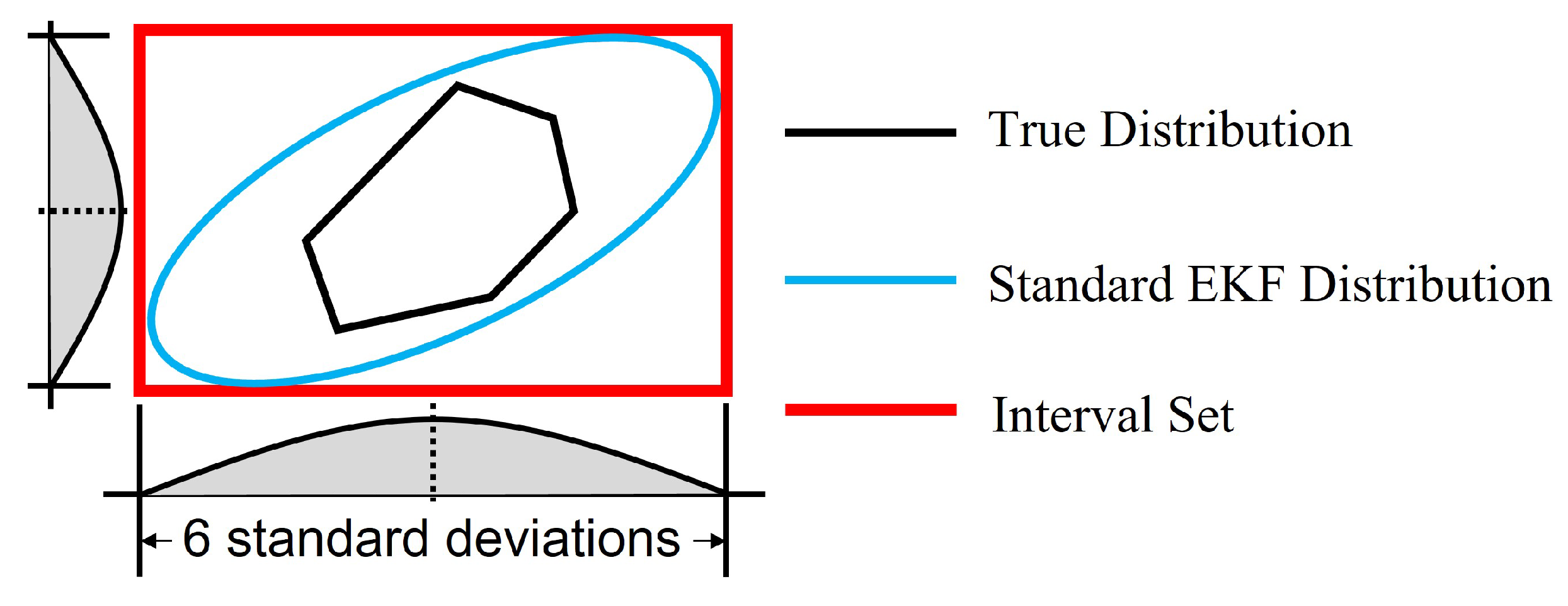
In this work, the noise was assumed to follow a truncated multivariate Gaussian distribution. The corresponding standard multivariate Gaussian distribution of noise contains the truncated one. As illustrated in Figure 1, when an EKF is used to estimate the states, the distribution of states with a standard Gaussian noise should similarly contain the one with the truncated Gaussian noise, which is the true distribution of states. Moreover, the distribution of states by standard EKF is also a multivariate Gaussian distribution. For Gaussian distribution, $99.7\%$ of the samples are within the interval of 6 standard deviations from both sides of the mean for each state. Thus, an interval set based on 6 standard deviations can contain the distribution by standard EKF and eventually contain the true distribution of states as in Figure 1. Since ${\mathit{P}}_{\mathit{k}}^{\mathit{i}}$ is the covariance of a standard EKF, the diagonal elements of matrix ${\mathit{P}}_{\mathit{k}}^{\mathit{i}}$ are the variances for each state. Therefore, diagonal elements of ${\mathit{P}}_{\mathit{k}}^{\mathit{i}}$ can be used to define the interval set to bound the error ${\mathit{ϵ}}_{\mathit{k}}^{\mathit{i}}$.

To formulate an error compensation operation scheme several set operations are introduced first as follows. The n-dimensional interval set is $\mathcal{S}(\mathit{p},\mathit{q})$ with lower bound $\mathit{p}$ and upper bound $\mathit{q}$ as $\mathcal{S}(\mathit{p},\mathit{q})=\{\mathit{x}\in {\mathbb{R}}^n:\mathit{p}\le \mathit{x}\le \mathit{q}\}$. The outer approximation operation $\mathcal{Q}(·)$ of a bounded set $\mathcal{W}$ is denoted by $\mathcal{Q}(\mathcal{W})$, which involves the mapping of the set $\mathcal{W}$ to a new interval set. If the infimum and supremum are denoted by $\inf (·)$ and $\sup (·)$, respectively, the outer approximation of the set $\mathcal{W}$ is $\mathcal{Q}(\mathcal{W})=\mathcal{S}(\inf (\mathcal{W}),\sup (\mathcal{W}))$. The operator ⊕ is the Minkowski addition of two sets. For example, for two sets $\alpha$ and $\beta$, $\alpha \oplus \beta =\{\mathit{a}+\mathit{b}:\forall \mathit{a}\in \alpha ,\forall \mathit{b}\in \beta \}$.

Notice that the diagonal elements of ${\mathit{P}}_{\mathit{k}}^{\mathit{i}}$ are the variances of each state. Then, if the standard deviation of ${\mathit{e}}_{\mathit{N},\mathit{k}}^{\mathit{i}}$ is ${\mathit{\eta }}_{\mathit{N},\mathit{k}}^{\mathit{i}}$ and of $e_{bio,k}^i$ is ${\eta }_{bio,k}^i$, two interval sets ${\mathcal{E}}_{N,k}$ and ${\mathcal{E}}_{bio,k}$ can be defined to bound ${\mathit{\eta }}_{\mathit{N},\mathit{k}}^{\mathit{i}}$ and ${\eta }_{bio,k}^i$, respectively, based on the choice of 3 standard deviation ranges, as ${\mathit{e}}_{\mathit{N},\mathit{k}}^{\mathit{i}}\in {\mathcal{E}}_{N,k}=\mathcal{S}(-3{\mathit{\eta }}_{\mathit{N},\mathit{k}}^{\mathit{i}},3{\mathit{\eta }}_{\mathit{N},\mathit{k}}^{\mathit{i}})$ and $e_{bio,k}^i\in {\mathcal{E}}_{bio,k}=\mathcal{S}(-3{\eta }_{bio,k}^i,3{\eta }_{bio,k}^i)$. In Equation (16b), since $|e_{bio,k}^i|<3{\eta }_{bio,k}^i$, we have $e_{bio,k}{\mathit{M}}_{\mathit{k}}{\mathit{e}}_{\mathit{N},\mathit{k}}^{\mathit{i}}\in 3{\eta }_{bio,k}^i{\mathit{M}}_{\mathit{k}}{\mathcal{E}}_{N,k}$. Similarly, the other two terms in Equation (16b) can be bounded as ${\mathit{D}}_{\mathit{k}}{\mathit{e}}_{\mathit{N},\mathit{k}}^{\mathit{i}}\in {\mathit{D}}_{\mathit{k}}{\mathcal{E}}_{N,k}$ and ${\mathit{L}}_{\mathit{k}}{e}_{bio,k}\in {\mathit{L}}_{\mathit{k}}{\mathcal{E}}_{bio,k}$, respectively. Therefore, the state deviation ${\mathit{ϵ}}_{\mathit{k}}^{\mathit{i}}$ term can be contained within the interval set ${\mathcal{E}}_{ϵ,k}$ according to Equation (18).

$${\mathit{ϵ}}_{\mathit{k}}^{\mathit{i}}\in {\mathcal{E}}_{ϵ,k}=\mathcal{Q}(({\mathit{D}}_{\mathit{k}}+3{\eta }_{bio,k}^i{\mathit{M}}_{\mathit{k}}){\mathcal{E}}_{N,k})\oplus \mathcal{Q}({\mathit{L}}_{\mathit{k}}{\mathcal{E}}_{bio,k})$$

(18)

where the sets ${\mathit{D}}_{\mathit{k}}{\mathcal{E}}_{N,k}$ and $3{\eta }_{bio,k}^i{\mathit{M}}_{\mathit{k}}{\mathcal{E}}_{N,k}$ occurring in Equation (18) are combined together. On the other hand, ${\mathit{L}}_{\mathit{k}}{\mathcal{E}}_{bio,k}$ originates from a different set ${\mathcal{E}}_{bio,k}$ and thus Minkowski addition must be used to add the different sets. However, linear mapping of interval sets can lead to irregular convex sets. In computational geometry, traditional algorithms that perform Minkowski addition for two convex irregular high-dimensional polytopes are computationally expensive [33]. On the other hand, Minkowski addition of two interval sets is computationally efficient because intervals are axis-aligned. Thus, the operator $\mathcal{Q}(·)$ that converts the irregular set to the axis-aligned set is applied to speed up the computation of the Minkowski addition.

Following the above, the set of states ${\widehat{\mathcal{X}}}_{k+1}$ is bounded by the prior estimate set ${\mathcal{P}}_{k+1}^{-}$ according to Equations (19a) and (19b).

$$\begin{array}{cc}\hfill {\mathcal{P}}_{k+1}^{-}& =\mathcal{Q}\{\underset{\mathrm{linear}\mathrm{mapping}}{\underbrace{\mathit{B}{\mathcal{P}}_k^{+}}}+\underset{\mathrm{translation}}{\underbrace{\Delta t{\widehat{x}}_{bio,k}\mathit{A}({\mathit{H}}_{\mathit{N}}^{\mathit{i}}{\mathit{\theta }}_{\mathit{N}}^{\mathit{i}}({\widehat{\mathit{x}}}_{\mathit{N},\mathit{k}}^{\mathit{i}})+{\mathit{g}}^{\mathit{i}})+\mathit{h}}}\}\oplus {\mathcal{E}}_{ϵ,k}\hfill \end{array}$$

(19a)

$$\begin{array}{cc}\hfill {\widehat{\mathcal{X}}}_{k+1}& \subset {\mathcal{P}}_{k+1}^{-}\hfill \end{array}$$

(19b)

where the set of the posterior estimates is ${\mathcal{P}}_k^{+}$. $\mathit{B}{\mathcal{P}}_k^{+}$ denotes the scaling of the set ${\mathcal{P}}_k^{+}$ by the diagonal matrix $\mathit{B}$. Then the set $\mathit{B}{\mathcal{P}}_k^{+}$ is translated by the vector in the big curly brackets. To compensate for the deviation during the convergence of EKF, the interval set ${\mathcal{E}}_{ϵ,k}$ is added by Minkowski addition.

Considering the truncated measurement noise, ${\mathit{r}}_{\mathit{k}}={\mathit{y}}_{\mathit{k}}-{\mathit{Cx}}_{\mathit{k}}$ is bounded by the lower $\mathit{l}$ and upper bounds $\mathit{u}$; let us define a set ${\mathcal{M}}_k=\{{\mathit{x}}_{\mathit{k}}\in {\mathbb{R}}^{n_x}:\mathit{l}<{\mathit{y}}_{\mathit{k}}-{\mathit{Cx}}_{\mathit{k}}<\mathit{u}\}$. Then, the posterior estimate set ${\mathcal{P}}_{k+1}^{+}$ is given by Equations (20a)–(20c). In this study, it is assumed that ${\mathcal{P}}_k^{+}$ and ${\mathcal{P}}_{k+1}^{-}$ are much smaller than the volumes of the critical regions.

$$\begin{array}{cc}\hfill {\mathcal{P}}_{k+1}^{+}& ={\mathcal{P}}_{k+1}^{-}\bigcap {\mathcal{M}}_{k+1}\hfill \end{array}$$

(20a)

$$\begin{array}{cc}\hfill {\widehat{\mathcal{X}}}_{k+1}& \subset {\mathcal{P}}_{k+1}^{+}\hfill \end{array}$$

(20b)

$$\begin{array}{cc}\hfill {\mathcal{P}}_0^{+}& ={\mathcal{P}}_0\hfill \end{array}$$

(20c)

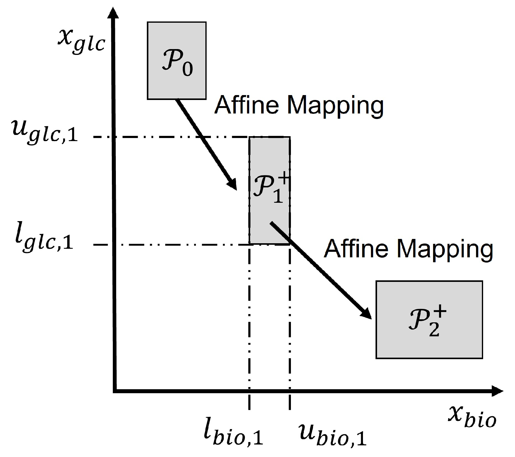
Figure 2 illustrates the set propagation using intervals for an example involving two states, e.g., glucose and biomass concentrations. The initial set ${\mathcal{P}}_0$ contains all possible initial values of glucose and biomass. Then ${\mathcal{P}}_1^{+}$ is generated through set operations by computational geometry algorithms. Since an interval set is used, it is computationally efficient to project the set ${\mathcal{P}}_1^{+}$ onto the biomass and glucose axes to obtain the corresponding lower bounds $l_{glc}$, $l_{bio}$ and upper bounds $u_{glc}$, $u_{bio}$ as shown in the figure for the set ${\mathcal{P}}_1^{+}$.

2.5. Detecting the Transition between Critical Regions

The proposed use of multiparametric programming converts the DFBM into a variable structure system composed of subsystems where each critical region corresponds to a subsystem. Along a given time trajectory the states may transit from one critical region to another. When the states estimated by the EKF leave a critical region ${\mathbf{\Theta }}^{\mathit{i}}$ to enter another critical region ${\mathbf{\Theta }}^{\mathit{j}}$, the estimate ${\widehat{\mathit{x}}}_{\mathit{M},\mathit{k}}$ and the covariance ${\mathit{P}}_{\mathit{k}}$ must be reinitialized because ${\mathit{x}}_{\mathit{M}}$ for different critical regions may be different, even though the measured states are the same. Moreover, a criterion is required to detect whether the states are entering into a new critical region.

When the system is traversing from one critical region to another, it needs to cross a boundary between the critical regions. Over time the states may cross over several boundaries along their trajectories and these crossings must be detected. Two neighboring critical regions share a boundary where an active constraint will become inactive or vice versa. The activation of a constraint may require the change of constraints related to ${\widehat{\mathit{x}}}_{\mathit{N},\mathit{k}}$. For a given constraint, $\theta$ is usually only function of two states at most because of commonly used Michaelis-–Menten kinetics [34] or constraints to prevent the depletion of nutrients [23] and one of these two states is biomass. So two special cases should be considered as follows when system switches from one critical region to the next:

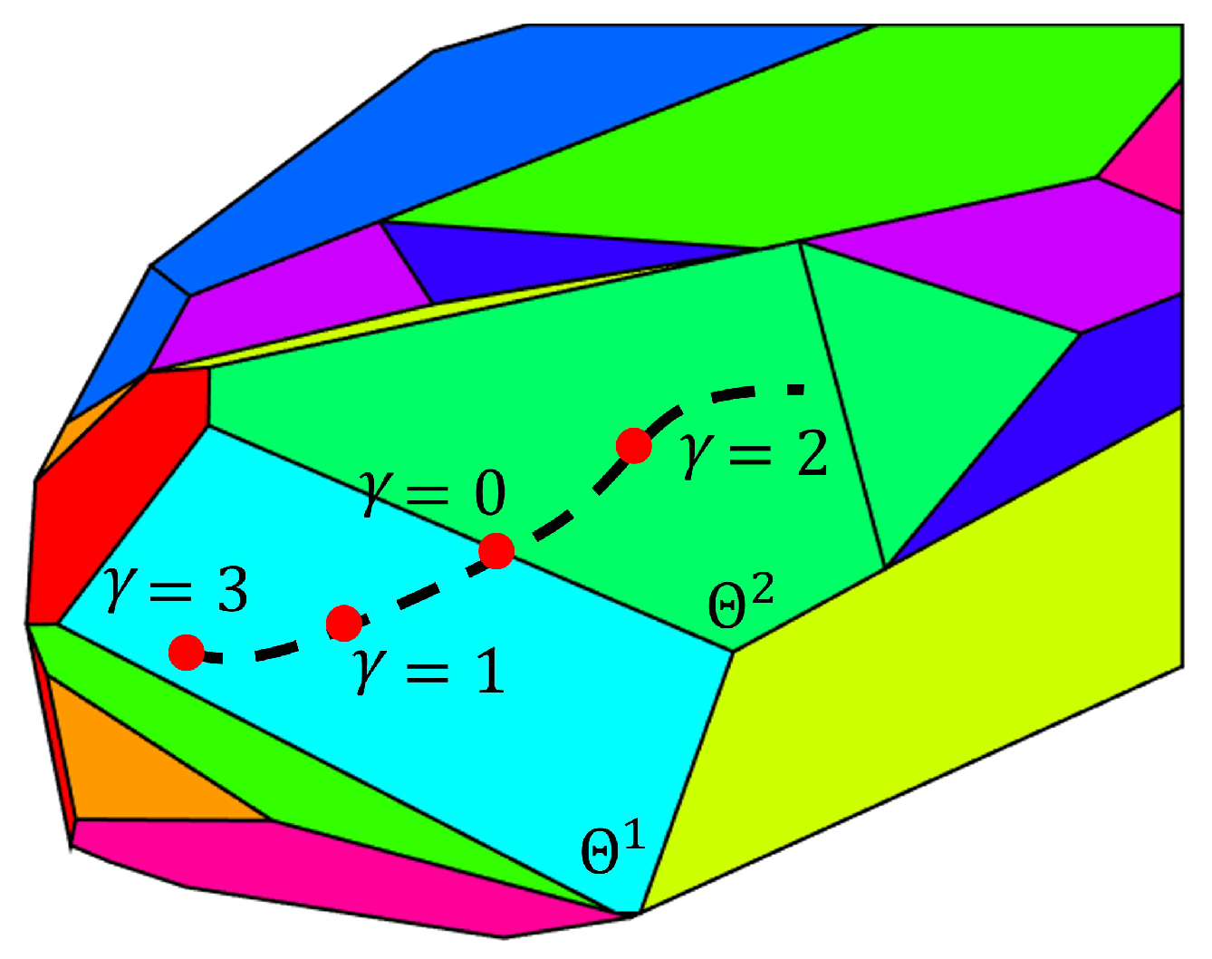
Case i—${\mathit{x}}_{\mathit{N}}^{\mathit{i}}$ of the old critical region ${\mathbf{\Theta }}^{\mathit{i}}$ have one more observable state than the ${\mathit{x}}_{\mathit{N}}^{\mathit{j}}$ of the new critical region ${\mathbf{\Theta }}^{\mathit{j}}$. For this case, the switch between critical regions is determined by Equation (21). Equation (21) calculates the norm of the difference between the flux estimates obtained with Equation (7) in the two neighboring regions. Notice that the flux estimate of ${\mathbf{\Theta }}^{\mathit{j}}$ is based on estimate ${\widehat{\mathit{x}}}_{\mathit{N},\mathit{k}}^{\mathit{i}}$ of the old critical region. The value of $\gamma (i,j,k)$ is used to detect the occurrence of a switch. If the system is exactly at the boundary of these two critical regions, the flux equation Equation (7) for these two critical regions should result in the same flux value and $\gamma (i,j,k)$ will be zero. A schematic example is shown in Figure 3. Polygons in different colors represent different critical regions in the parameter space $\mathbf{\Theta }$. As the state evolves with time, the corresponding $\mathit{\theta }$ changes along the dash line in the parameter space $\mathbf{\Theta }$. As the $\mathit{\theta }$ approaches the boundary between the critical region ${\mathbf{\Theta }}^{\mathbf{1}}$ and ${\mathbf{\Theta }}^{\mathbf{2}}$, $\gamma (i,j,k)$ approaches zero. Correspondingly, a value of $\gamma (i,j,k)$ smaller than a user specified tolerance indicates a switch between critical regions, thus requiring reinitialization of the EKF as follows: ${\widehat{\mathit{x}}}_{\mathit{N},\mathit{k}}^{\mathit{j}}$ is set equal to ${\widehat{\mathit{x}}}_{\mathit{N},\mathit{k}}^{\mathit{i}}$ and ${\mathit{P}}_{\mathit{k}}^{\mathit{j}}$ is set equal to ${\mathit{P}}_{\mathit{k}}^{\mathit{i}}$.

$$\gamma (i,j,k)=∥{\widehat{\mathit{v}}}_{\mathit{k}}^{\mathit{i}}-{\widehat{\mathit{v}}}_{\mathit{k}}^{\mathit{j}}∥=∥{\mathit{H}}_{\mathit{N}}^{\mathit{i}}{\mathit{\theta }}_{\mathit{N}}^{\mathit{i}}({\widehat{\mathit{x}}}_{\mathit{N},\mathit{k}}^{\mathit{i}})+{\mathit{g}}^{\mathit{i}}-({\mathit{H}}_{\mathit{N}}^{\mathit{j}}{\mathit{\theta }}_{\mathit{N}}^{\mathit{j}}({\widehat{\mathit{x}}}_{\mathit{N},\mathit{k}}^{\mathit{i}})-{\mathit{g}}^{\mathit{j}})∥$$

(21)

Case ii—${\mathit{x}}_{\mathit{N}}^{\mathit{j}}$ of the new critical region ${\mathbf{\Theta }}^{\mathit{i}}$ has one more observable state than the ${\mathit{x}}_{\mathit{N}}^{\mathit{j}}$ of the old critical region ${\mathbf{\Theta }}^{\mathit{i}}$. To reinitialize the EKF, ${\widehat{\mathit{x}}}_{\mathit{N},\mathit{k}}^{\mathit{j}}$ and ${\mathit{P}}_{\mathit{k}}^{\mathit{j}}$ can be set to the old values except for the new observable state that is not observable in the old critical region, and thus it needs to be estimated for calculating $\gamma (i,j,k)$. By projecting the set ${\mathcal{P}}_k^{+}$, the lower $l_{un,k}$ and upper bounds $u_{un,k}$ can be calculated. Since no extra information is available, the mean value of the upper bound and lower bound is used as the nominal value of the unobservable state as per Equation (22).

$${\widehat{x}}_{un,k}^i=\frac{1}{2}(u_{un,k}+l_{un,k})$$

(22)

Equation (23) is used to calculate $\gamma (i,j,k)$. The flux estimate for the new critical region ${\mathbf{\Theta }}^{\mathit{j}}$ is based on the nominal values of the unobservable state ${\widehat{x}}_{un,k}^i$ combined with ${\widehat{x}}_{N,k}^i$ of the old critical region.

$$\gamma (i,j,k)=∥{\widehat{\mathit{v}}}_{\mathit{k}}^{\mathit{i}}-{\widehat{\mathit{v}}}_{\mathit{k}}^{\mathit{j}}∥=∥{\mathit{H}}_{\mathit{N}}^{\mathit{i}}{\mathit{\theta }}_{\mathit{N}}^{\mathit{i}}({\widehat{\mathit{x}}}_{\mathit{N},\mathit{k}}^{\mathit{i}})+{\mathit{g}}^{\mathit{i}}-({\mathit{H}}_{\mathit{N}}^{\mathit{j}}{\mathit{\theta }}_{\mathit{N}}^{\mathit{j}}({\widehat{x}}_{un,k}^i,{\widehat{\mathit{x}}}_{\mathit{N},\mathit{k}}^{\mathit{i}})-{\mathit{g}}^{\mathit{j}})∥$$

(23)

To reinitialize the EKF, the estimate and covariance are used together with the estimation of the new state that is added in the new critical region. Assuming the states are close enough to the boundary between the critical regions, then Equation (24) holds.

$$∥{\mathit{H}}_{\mathit{N}}^{\mathit{i}}{\mathit{\theta }}_{\mathit{N}}^{\mathit{i}}({\widehat{\mathit{x}}}_{\mathit{N},\mathit{k}}^{\mathit{i}})+{\mathit{g}}^{\mathit{i}}-({\mathit{H}}_{\mathit{N}}^{\mathit{j}}{\mathit{\theta }}_{\mathit{N}}^{\mathit{j}}({\widehat{x}}_{N,k}^j,{\widehat{x}}_{un,0}^j)-{\mathit{g}}^{\mathit{j}})∥=0$$

(24)

The initial estimate of new observable state ${\widehat{x}}_{un,0}^j$ in the new region can be calculated by solving the Equation (24). Since the new state is between the upper bound and lower bound by SME, the half length between $u_{un,k}$ and $l_{un,k}$ is the worst possible deviation. Then, using a 3 standard deviation range, the initial variance ${\eta }_{un,k}^2$ can be estimated according to Equation (25) and all other covariance terms related to the new state are assumed to be zero.

$${\eta }_{un,k}=\frac{1}{3}·\frac{1}{2}(u_{un,k}-l_{un,k})$$

(25)

Bounds of states estimated by the SME are rigorously guaranteed in each critical region separately but subject to accurate tuning of the tolerance that is used to switch between the subsystems. The tolerance of $\gamma (i,j,k)$ is the only user specified parameter in this research. If the tolerance is too large or small, the EKF may switch the subsystem too early or too late. Accordingly, if the wrong state equations are used in estimation, the bounds on the states may be violated. To avoid such a situation, exhaustive simulations that are initialized with ${\mathcal{P}}_0$ are conducted to find the tolerance used to switch between critical regions. As an alternative, an overestimated covariance can also be used to reinitialize the EKF when the state enters a new critical region to avoid bound violations.

3. Results

3.1. DFBM Model of E. coli

A DFBM model of E. coli reported in [20] is used to illustrate the proposed methodology. The DFBM in batch operation includes four states, glucose concentration $x_{glc}$, oxygen concentration $x_{oxy}$, acetate concentration $x_{ace}$, and biomass concentration $x_{bio}$ as in Equations (26a)–(26e). Thus, the state vector is $\mathit{x}={\left[\begin{array}{cccc}{x}_{glc}& x_{oxy}& x_{ace}& x_{bio}\end{array}\right]}^T$. The substrates are glucose, oxygen, acetate.

$$\begin{array}{cc}\hfill x_{glc,k+1}& =x_{glc,k}+\Delta t{x}_{bio,k}{\mathit{A}}_{\mathit{glc}}{\mathit{v}}_{\mathit{k}}\hfill \end{array}$$

(26a)

$$\begin{array}{cc}\hfill x_{oxy,k+1}& =(1-k_{L}a\Delta t)x_{oxy,k}+\Delta t{x}_{bio,k}{\mathit{A}}_{\mathit{oxy}}{\mathit{v}}_{\mathit{k}}+0.21k_{L}a\Delta t\hfill \end{array}$$

(26b)

$$\begin{array}{cc}\hfill x_{ace,k+1}& =x_{ace,k}+\Delta t{x}_{bio,k}{\mathit{A}}_{\mathit{ace}}{\mathit{v}}_{\mathit{k}}\hfill \end{array}$$

(26c)

$$\begin{array}{cc}\hfill x_{bio,k+1}& =x_{bio,k}+\Delta t{x}_{bio,k}{\mathit{A}}_{\mathit{bio}}{\mathit{v}}_{\mathit{k}}\hfill \end{array}$$

(26d)

$$\begin{array}{cc}\hfill {\mathit{x}}_{\mathbf{0}}& \in {\mathcal{P}}_0=\mathcal{S}({\left[\begin{array}{cccc}0.38& 0.1995& 0.19& 0.00095\end{array}\right]}^T,{\left[\begin{array}{cccc}0.42& 0.2205& 0.21& 0.00105\end{array}\right]}^T)\hfill \end{array}$$

(26e)

where $k_{L}a=4h^{-1}$ is the oxygen mass transfer coefficient. The initial state vector ${\mathit{x}}_{\mathbf{0}}$ is defined by the interval set ${\mathcal{P}}_0$ according to Equation (26e). The matrix A contains the stoichiometric coefficients corresponding to four reactions according to Equation (27). Each column of this matrix corresponds to one reaction and each row correspond to one component.

$$\mathit{A}=\left[\begin{array}{c}{\mathit{A}}_{\mathit{glc}}\\ {\mathit{A}}_{\mathit{oxy}}\\ {\mathit{A}}_{\mathit{ace}}\\ {\mathit{A}}_{\mathit{bio}}\end{array}\right]=\left[\begin{array}{cccc}0& -9.46& -9.84& -19.23\\ -35& -12.92& -12.73& 0\\ -39.43& 0& 1.24& 12.12\\ 1& 1& 1& 1\end{array}\right]$$

(27)

The flux vector ${\mathit{v}}_{\mathit{k}}$ is obtained by solving the following linear programming problem as Equations (28a)–(28g):

$$\begin{array}{ccccc}\hfill & \underset{{\mathit{v}}_{\mathit{k}}}{max}\hfill & \hfill & {\mathit{A}}_{\mathit{bio}}{\mathit{v}}_{\mathit{k}}\hfill & \end{array}$$

(28a)

$$\begin{array}{ccccc}\hfill & \mathrm{subject}\mathrm{to}\hfill & \hfill & -{\mathit{A}}_{\mathit{oxy}}{\mathit{v}}_{\mathit{k}}\le {\mathrm{OUR}}_{max}\hfill & \end{array}$$

(28b)

$$\begin{array}{ccccc}\hfill & \hfill & & {\mathit{A}}_{\mathit{ace}}{\mathit{v}}_{\mathit{k}}\le 100\hfill & \end{array}$$

(28c)

$$\begin{array}{ccccc}\hfill & \hfill & & -\Delta t{\mathit{A}}_{\mathit{glc}}{\mathit{v}}_{\mathit{k}}\le \frac{x_{glc,k}}{x_{bio,k}}={\theta }_{1,k}\hfill & \end{array}$$

(28d)

$$\begin{array}{ccccc}\hfill & \hfill & & -\Delta t{\mathit{A}}_{\mathit{oxy}}{\mathit{v}}_{\mathit{k}}\le \frac{(1-k_{L}a\Delta t)x_{oxy,k}+0.21k_{L}a\Delta t}{x_{bio,k}}={\theta }_{2,k}\hfill & \end{array}$$

(28e)

$$\begin{array}{ccccc}\hfill & \hfill & & -\Delta t{\mathit{A}}_{\mathit{ace}}{\mathit{v}}_{\mathit{k}}\le \frac{x_{ace,k}}{x_{bio,k}}={\theta }_{3,k}\hfill & \end{array}$$

(28f)

$$\begin{array}{cccc}\hfill & \hfill & & -{\mathit{A}}_{\mathit{glc}}{\mathit{v}}_{\mathit{k}}\le \frac{{\mathrm{GUR}}_{max}{x}_{glc,k}}{K_m+x_{glc,k}}={\theta }_{4,k}\hfill \end{array}$$

(28g)

where ${\mathrm{OUR}}_{max}=12\mathrm{mM}/(\text{g−dw}·\mathrm{h})$ is the maximum oxygen uptake rate and g-dw is grams of dry weight of biomass; ${\mathrm{GUR}}_{max}=6.5\mathrm{mM}/(\text{g−dw}·\mathrm{h})$ denotes the maximum glucose uptake rate. Equation (28a) describes that the objective of the cells is to maximize the biomass growth rate. Equation (28b) indicates that the oxygen consumption rate is limited by a maximum uptake limit. Equation (28c) indicates that the acetate generation rate is bounded by $100\mathrm{mM}/(\text{g−dw}·\mathrm{h})$. Equation (28g) indicates that the glucose consumption rate is bounded by an upper limit. All the other constraints are positivity constraints to prevent depletion of metabolites. To express these constraints in Equations (28a)–(28g) compactly, the constraints in (28a)–(28g) can be expressed in the form of Equation (3):

$$\begin{array}{cc}\hfill {\mathit{Gv}}_{\mathit{k}}& \le \mathit{F}{\mathit{\theta }}_{\mathit{k}}({\mathit{x}}_{\mathit{k}})+\mathit{z}\hfill \end{array}$$

(29a)

$$\begin{array}{cc}\hfill \mathit{G}& =\left[\begin{array}{c}-{\mathit{A}}_{\mathit{oxy}}\\ {\mathit{A}}_{\mathit{ace}}\\ -\Delta t{\mathit{A}}_{\mathit{glc}}\\ -\Delta t{\mathit{A}}_{\mathit{oxy}}\\ -\Delta t{\mathit{A}}_{\mathit{ace}}\\ -{\mathit{A}}_{\mathit{glc}}\end{array}\right]\hfill \end{array}$$

(29b)

$$\begin{array}{cc}\hfill \mathit{F}& =\left[\begin{array}{cccc}0& 0& 0& 0\\ 0& 0& 0& 0\\ 1& 0& 0& 0\\ 0& 1& 0& 0\\ 0& 0& 1& 0\\ 0& 0& 0& 1\end{array}\right]\hfill \end{array}$$

(29c)

$$\begin{array}{cc}\hfill \mathit{z}& =\left[\begin{array}{c}{\mathrm{OUR}}_{max}\\ 100\\ 0\\ 0\\ 0\\ 0\end{array}\right]\hfill \end{array}$$

(29d)

3.2. Determination of Minimum Measurements

Due to the assumption that the initial state is contained in an interval, the problem in Equations (28a)–(28g) can be formulated as a multiparameteric linear programming (mpLP) problem. The vector $\mathit{\theta }$ is composed of four parameters which are nonlinear functions of states. Using the Multi-Parametric Toolbox 3.0, it can be found that the entire parameter space $\mathbf{\Theta }$ can be decomposed into a maximum of 24 critical regions. For each critical region, the mpLP solver calculates the constraints that form the boundaries of the region and the equations that generate the optimal solutions. In order to reduce the computational effort, extensive simulations are conducted with randomly chosen initial values in set ${\mathcal{P}}_0$ to identify which critical regions are relevant for the problem. It is found from these simulations that, for the chosen range of initial conditions, the states only traverse through two neighboring critical regions ${\mathbf{\Theta }}^1$ and ${\mathbf{\Theta }}^2$ assuming small critical regions are ignored. According to the results of the mpLP solver, the two critical regions can be defined as Equations (30a) and (30b). Critical regions ${\mathbf{\Theta }}^1$ and ${\mathbf{\Theta }}^2$ share a boundary defined in Equation (30c). Since $\mathit{\theta }$ is a function of $\mathit{x}$, the critical regions are next to each other in the state space.

$$\begin{array}{cc}\hfill {\mathbf{\Theta }}^1:\left[\begin{array}{ccccc}-0.9988& 0& 0& 0.0499& 0\\ 0& -1& 0& 0& 0\\ 0& 0& -0.9971& -0.0767& 0\\ 0& 0& 0& -0.0033& -1\\ 0& 0& 0& 1& 0\\ 0& 0& 0& -1& 0\end{array}\right]\mathit{\theta }(\mathit{x})& \le \left[\begin{array}{c}0\\ -0.6\\ -0.6740\\ 0.0171\\ 8.7864\\ 0\end{array}\right]\hfill \end{array}$$

(30a)

$$\begin{array}{cc}\hfill {\mathbf{\Theta }}^2:\left[\begin{array}{ccccc}-0.9988& 0& 0& 0.0499& 0\\ 0& -0.7469& 0.6630& 0.0510& 0\\ 0& 0& -0.0254& -0.0053& -0.9997\\ 0& 0& -1& 0& 0\\ 0& 0& 0.9971& 0.0767& 0\\ 0& 0& 0& -1& 0\end{array}\right]\mathit{\theta }(\mathit{x})& \le \left[\begin{array}{c}0\\ 0\\ 0\\ 0\\ 0.6740\\ 0\end{array}\right]\hfill \end{array}$$

(30b)

$$\begin{array}{cc}\hfill {\mathbf{\Theta }}^1\bigcap {\mathbf{\Theta }}^2:\left[\begin{array}{ccccc}0& 0& 0.9971& 0.0767& 0\end{array}\right]\mathit{\theta }(\mathit{x})& =0.6740\hfill \end{array}$$

(30c)

Accordingly, the mpLP solver also calculates the matrix $\mathit{H}$ and $\mathit{g}$ used in the flux equation Equation (7) for these two critical regions. By taking advantage of the sparseness of $\mathit{H}$ for these two critical regions, ${\mathit{\theta }}_{\mathit{N}}$ can be determined. The equations to calculate fluxes for these two critical regions can be expressed as Equations (31a) and (31b).

$$\begin{array}{cc}\hfill {\mathit{v}}_{\mathit{k}}^{\mathbf{1}}& ={\left[\begin{array}{cccc}-0.039& 0.1057& 0& 0\end{array}\right]}^T{\theta }_4(x_{glc,k})+{\left[\begin{array}{cccc}0.3429& 0& 0& 0\end{array}\right]}^T\hfill \end{array}$$

(31a)

$$\begin{array}{cc}\hfill {\mathit{v}}_{\mathit{k}}^{\mathbf{2}}& ={\left[\begin{array}{cccc}0.5072& 0& 0& 0\end{array}\right]}^T{\theta }_3(x_{ace,k},x_{bio,k})+{\left[\begin{array}{cccc}0& 0.1057& 0& 0\end{array}\right]}^T{\theta }_4(x_{glc,k})\hfill \end{array}$$

(31b)

where ${\mathit{\theta }}_{\mathit{N}}$ for critical region ${\mathbf{\Theta }}^1$ is ${\theta }_4$ and ${\mathit{\theta }}_{\mathit{N}}$ for critical region ${\mathbf{\Theta }}^2$ is ${\theta }_3$ and ${\theta }_4$. By substituting the flux equation Equations (31a) and (31b) into Equations (26a)–(26e), the simplified state equations of E. coli model can be rewritten compactly as in Equations (32a) and (32b).

$$\begin{array}{ccc}\hfill {\mathit{x}}_{\mathit{k}+\mathbf{1}}& =\mathit{B}{\mathit{x}}_{\mathit{k}}+\Delta t{x}_{bio,k}{\mathit{Av}}_{\mathit{k}}^{\mathbf{1}}(x_{glc,k})+\mathit{h}\hfill & \hfill \mathit{\theta }({\mathit{x}}_{\mathit{k}})\in {\mathbf{\Theta }}^1\end{array}$$

(32a)

$$\begin{array}{ccc}\hfill {\mathit{x}}_{\mathit{k}+\mathbf{1}}& =\mathit{B}{\mathit{x}}_{\mathit{k}}+\Delta t{x}_{bio,k}{\mathit{Av}}_{\mathit{k}}^{\mathbf{2}}(x_{ace,k},x_{bio,k},x_{glc,k})+\mathit{h}\hfill & \hfill \mathit{\theta }({\mathit{x}}_{\mathit{k}})\in {\mathbf{\Theta }}^2\end{array}$$

(32b)

Following the calculations above, the original E. coli model is simplified into an equivalent system comprised of two subsystems of interest. Equations (32a) and (32b) describe subsystem 1 and subsystem 2, respectively. These two subsystems are continuous in the state space and they share the same boundary as per Equation (30c). Once the state crosses the boundary between the two subsystems, the governing equation is switched from Equations (32a) and (32b). Because the initial state is randomly initialized in set ${\mathcal{P}}_0$, ${\mathcal{P}}_0$ corresponds to a set in ${\mathbf{\Theta }}^1$. Thus, the state evolves within the region of subsystem 1 and gradually approximates the region of subsystem 2 governed by Equation (32b) until finally crossing the boundary given by Equation (30c). As only part of $\theta$ is known, a detector is used to detect the crossing of the boundary, thus ensuring that the switch between the regions is performed accurately.

Based on the flux equation Equations (31a) and (31b), the reaction-rate-determining states vector ${\mathit{x}}_{\mathit{M}}^{\mathit{i}}$ for ${\mathbf{\Theta }}^1$ are biomass and glucose and for ${\mathbf{\Theta }}^2$ are biomass, acetate and glucose. Accordingly, the possible combinations of measurements needed for observing ${{\mathit{x}}_{\mathit{M}}}^1$ of ${\mathbf{\Theta }}^1$ include ${\Omega }_1^1=\{Bio\}$, ${\Omega }_2^1=\{Glc\}$ and ${\Omega }_3^1=\{Bio,Glc\}$. Similarly, there are 7 possible combinations of measurements for observing the vector ${{\mathit{x}}_{\mathit{M}}}^2$ in ${\mathbf{\Theta }}^2$, namely ${\Omega }_1^2=\{Ace\}$, ${\Omega }_2^2=\{Bio\}$, ${\Omega }_3^2=\{Glc\}$, ${\Omega }_4^2=\{Ace,Bio\}$, ${\Omega }_5^2=\{Bio,Glc\}$, ${\Omega }_6^2=\{Ace,Glc\}$, and ${\Omega }_7^2=\{Ace,Bio,Glc\}$. To find a combination of measurements ${\Omega }_{\Gamma }$ that will be suitable for both critical regions, it is necessary to perform an analysis of observability for these combinations. The Symbolic Toolbox calculation of MATLAB R2018a is used to develop an analytical equation observability rank condition and rank of ${\mathsf{\Phi }}_{\mathit{k}}^{\mathit{i}}$ of the nonlinear system according to the criterion presented in [31]. Since the symbolic expressions of the rank for each critical regions for Equation (11) are very complex, it is very difficult to infer a analytical condition of observability for all possible values of the states. Instead, the rank values are calculated for different measurement combinations and rank of ${\mathsf{\Phi }}_{\mathit{k}}^{\mathit{i}}$ using a Monte Carlo algorithm based on 5 million samples of ${\mathbf{\Theta }}^1$ and ${\mathbf{\Theta }}^2$, respectively. According to these Monte Carlo simulations, the only measurement required for observability of the vectors ${\mathit{x}}_{\mathit{M}}^{\mathbf{1}}$ in ${\mathbf{\Theta }}^1$ and ${\mathit{x}}_{\mathit{M}}^{\mathbf{2}}$ in ${\mathbf{\Theta }}^2$ is the biomass concentration, namely ${\Omega }_{\Gamma }=\{Bio\}$.

3.3. EKF for the Two Subsystems and Detection of Transition between Subsystems

Based on the aforementioned observability analysis, the biomass concentration is the only state that needs to be measured online as per Equation (33a) for implementation of the EKF. Measurement noise is assumed as a truncated normal distribution as described by Equation (33b). Since the initial ${\mathcal{P}}_0$ is assumed to be known, the EKF is initialized at the center of ${\mathcal{P}}_0$ with a variance based on 3 standard deviations and zero covariance terms. The state of the plant is initialized randomly by sampling a point within the region defined by ${\mathcal{P}}_0$.

$$\begin{array}{cc}\hfill y_k& =\left[\begin{array}{cccc}0& 0& 0& 1\end{array}\right]{\mathit{x}}_{\mathit{k}}+r_k\hfill \end{array}$$

(33a)

$$\begin{array}{cc}\hfill r_k& \sim TN(0,0.{004}^2,-0.0004,0.0004)k=0,1,2\cdots \hfill \end{array}$$

(33b)

Based on the assumed ${\mathcal{P}}_0$, in the batch process the EKF starts in critical region ${\mathbf{\Theta }}^1$ and later it transitions into critical region ${\mathbf{\Theta }}^2$. Thus, two EKFs are required in this case study to estimate the ${\mathit{x}}_{\mathit{M}}$ as summarized in

Table 1. Observable and unobservable subpace of two subsystems of the DFBM model of E. coli.

	Subsystem of ${\mathbf{\Theta }}^1$	Subsystem of ${\mathbf{\Theta }}^2$
Observable Subspace (${\mathit{x}}_{\mathit{M}}$)	Glc, Bio	Glc, Ace, Bio
Unobservable Subspace	Ace, Oxy	Oxy
Measurement	Bio	Bio

. Based on the biomass measurement $y_k$, the glucose and biomass concentrations are estimated by the EKF for ${\mathbf{\Theta }}^1$ as ${\widehat{x}}_{N,bio,k}$ and ${\widehat{x}}_{N,glc,k}$. With the same biomass measurement, the second critical region ${\mathbf{\Theta }}^2$ has one more observable state which is the acetate concentration ${\widehat{x}}_{N,ace,k}$.

Since acetate and oxygen are unobservable in ${\mathbf{\Theta }}^1$, they need to be estimated by bounds. To find these bounds, SME propagates the initial set ${\mathcal{P}}_0$ by set operations to obtain a prior estimate set ${\mathcal{P}}_k^{-}$ as Equation (19). After obtaining the measurement of biomass, a posterior estimate set ${\mathcal{P}}_k^{+}$ as in Equation (20) is calculated by set operations. The error due to lack of convergence of the EKF is compensated by using Equation (18). By projecting ${\mathcal{P}}_k^{+}$ onto the axis of acetate and oxygen, respectively, the upper bound ${\mathit{u}}_{\mathit{un},\mathit{k}}$ and lower bound ${\mathit{l}}_{\mathit{un},\mathit{k}}$ of these two states are obtained.

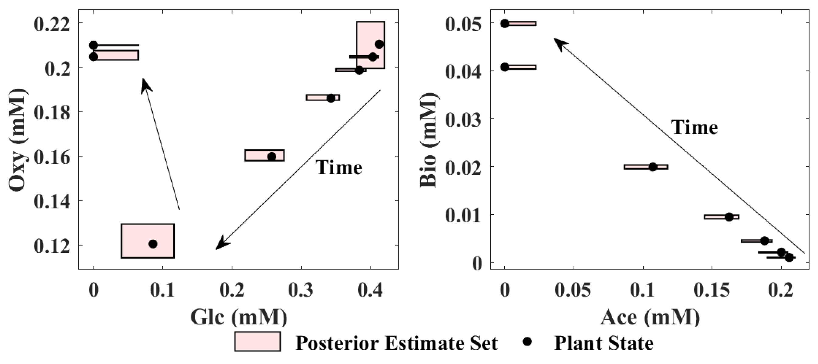
Since ${\mathbf{\Theta }}^2$ has one more flux-determining state, acetate that is not observable from the measurement of biomass, it must be estimated as explained in Equation (22). Using the mean value of $u_{un,ace,k}$ and $l_{un,ace,k}$ the nominal values of the unobservable state ${\widehat{x}}_{un,ace,k}$ are obtained. Using the EKF estimates of the observable flux-determining states ${\widehat{\mathit{x}}}_{\mathit{N},\mathit{k}}$ together with the nominal value of acetate ${\widehat{x}}_{un,ace,k}$, the detection scheme explained in Section 2.5 can be implemented. Accordingly, $\gamma (i,j,k)$ is calculated from Equation (23) to determine the switch from critical region ${\mathbf{\Theta }}^1$ to critical region ${\mathbf{\Theta }}^2$. The tolerance of $\gamma (i,j,k)$ to determine the switch between the critical regions is assumed as 0.08. This tolerance is the only tuning parameter of the proposed method and it is determined by trial and error. After the switch occurs the acetate concentration is initialized by the solution of Equation (24) and the variance of acetate is initialized based on Equation (25). After the switch to critical region ${\mathbf{\Theta }}^2$, the EKF continues to generate estimates of glucose, acetate and biomass concentrations in ${\mathbf{\Theta }}^2$ and the SME approach is used to propagate the set ${\mathcal{P}}_k^{+}$ as conducted in critical region 1. Figure 4 presents the posterior estimate sets ${\mathcal{P}}^{+}$ and true plant state $\mathit{x}$ at different times. Since the model is 4 dimensional, the posterior estimate sets ${\mathcal{P}}^{+}$ are projected for visualization onto two dimensional spaces: the glucose–oxygen subspace and acetate–biomass subspace. The 8 boxes denote the projected posterior estimate sets between 0 h and 7 h, and each box represents an hour. The arrows in Figure 4 indicate the direction of time evolution. The black dots denote the true plant state. Since biomass is measured, the length of the boxes along the biomass dimension is relatively smaller, as compared to the other dimensions. The switch between the critical regions occurs at around 5 h.

3.4. Set Membership Estimation

To verify the estimate and bounds generated by the proposed algorithm, we use a special Monte Carlo Algorithm (MCA) that takes biomass measurements into account. MCA randomly samples 100,000 different points from ${\mathcal{P}}_0$ and use them as initial states’ values, and then calculates the corresponding trajectories with respect to time. Since, for the measurement of biomass, a truncated normal distribution measurement noise was assumed, some trajectories are not within the confidence interval of measurements. Once a trajectory is found out of the measurement range, the evolution of the trajectory is stopped and the corresponding trajectory is removed while trajectories which are still within the confidence interval of measurements are kept. Accordingly, only a part (2581) out of the trajectories starting from ${\mathcal{P}}_0$ are used for comparison to the bounds calculated by the proposed method. It should be noticed the fraction of trajectories kept for comparison is small because only a very narrow set of solutions are within the measurement range from the from the beginning to the end. In other words, only a small part of the samples considered in the simulation are compatible with the biomass measured trajectory that is assumed for the calculation of bounds by the set-based approach. Using parallel computation, 4 h and 4 min of CPU time were required to complete all simulations. For comparison, the method proposed in this work can generate bounds with only 41 s of CPU time without parallel computation. It should be remembered that the MCA was conducted for a specific trajectory of biomass measurements so as to enable a fair comparison with the method proposed in the current study. While it could be argued that MCA could be used to calculate bounds for all possible biomass trajectories, this will be computationally prohibitive. Thus, the proposed technique is a practical and analytical approach to the online estimation problem.

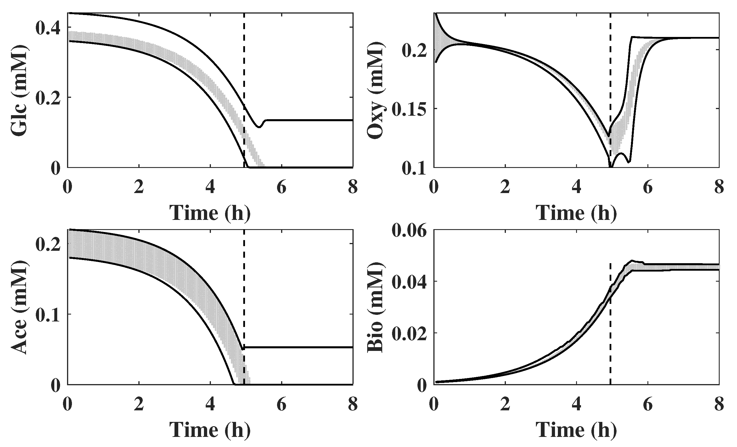
In Figure 5, the grey area denotes the trajectories randomly sampled and the two black lines represent the upper and lower bounds by SME. It is clear that the SME contains all the solutions generated by MCA, especially for the unobservable states. It can be observed that the switch from one critical region to the other occurs at approximately 5 h as shown in Figure 2. Before 5 h, the reactor has enough resources for cell growth and the limiting step is glucose uptake as Equation (31a) shows. Thus, critical region ${\mathbf{\Theta }}^1$ corresponds to the logarithmic phase of growth where the latter is driven by glucose consumption. At about 5 h, the simultaneous depletion of acetate and glucose leads to a metabolic switch from the logarithmic phase to the stationary phase. Following this metabolic switch, the culture is also acetate limited and thus acetate become a new flux-determining state. Since the oxygen feed rate is maintained constant in the model, the fact that the growth significantly decreases after the switch explains why the oxygen concentration bounces back up.

To further verify the proposed scheme, similar MCA simulations were conducted with a larger initial uncertainty and measurement noise. In Figure 6, the bounds of 4 component concentrations estimated by SME are shown. It is clear that the simulated trajectories contained in the grey color band generated by MCA is within the bounds calculated by the proposed methodology. From comparison of Figure 5 and Figure 6, it can be found that the SME approach copes with the larger noise and initial uncertainty by generating larger bounds.

4. Discussion

DFBM models are advantageous since they contain significant detail about the cell metabolism as compared to classical unstructured models. However, due to this level of detail, DFBM contain many states thus resulting in more difficult state estimation problem. The challenge of dealing with a large number of states is further exacerbated by the fact that online measurements of metabolites are generally difficult to obtain or not available. With limited online measurements, it is often impossible to produce observability for all the states. Noticing that the diagonal matrix $\mathit{B}$ in Equation (19) is a linear mapping of states, if the nonlinear term $\Delta t{x}_{bio,k}{\mathit{Av}}_{\mathit{k}}$ can be estimated then it is possible to estimate the other states of the DFBM.

Multiparametric LP is introduced to convert the original system into a series of piecewise continuous subsystems based on the partitioning of the parameter space into critical regions. The availability of an explicit expression for the calculation of the LP optima for each critical region significantly simplifies the solution of the problem. Although many critical regions may be mathematically possible, industrial fermentation is operated in a narrow range of initial operating conditions and as such only a few critical regions need to be considered.

Beyond their computational convenience the critical regions identified by the Multiparametric LP approach can be interpreted as corresponding changes in the cell metabolism. The relative abundance of substrates, i.e., glucose, acetate and oxygen in the E. coli model and their consumption towards biomass lead to the occurrence of different resources’ limitations at any given time. Within some ranges of concentration, the limiting substrate remains the same corresponding to a specific metabolism strategy.

In the E. coli example, four reactions can synthesize the biomass from glucose, acetate and oxygen. However, since the objective is to maximize growth subject to constraints, the cell prioritizes these reactions differently at any given time due to their different efficiency for biomass synthesis. The ratio of the stoichiometry coefficients in each column of matrix $\mathit{A}$ indicates the biomass yield of each substrate for each reaction. Reaction 1 is the only reaction that consumes acetate to synthesize biomass. The yield of acetate to biomass is $\frac{1}{39.43}$ for reaction 1, which is very low compared with reaction 2 and reaction 3. The biomass yield of reaction 2 and reaction 3 by glucose is $\frac{1}{9.46}$ and $\frac{1}{9.84}$, respectively. Reaction 4 is the only reaction that do not consume oxygen to generate biomass but it is very inefficient. Because the biomass yield of these reactions are different, reaction 2 is preferred over reaction 1 and reaction 3 when glucose and oxygen are abundant. When oxygen is very low, the cells switch their metabolism from aerobic to anaerobic to generate biomass through reaction 4.

To maximize the biomass growth rate, cells take advantage of reaction 1 and 2 to consume as much acetate and glucose as possible when oxygen is sufficient. However, the glucose amounts that can be consumed by the cells is limited by the glucose uptake rate, which is ${\theta }_4$. Similarly, oxygen consumption is limited by a constant oxygen uptake rate as in Equation (28b). The oxygen is consumed first with glucose in reaction 2 to synthesize biomass and the remaining oxygen is consumed for reaction 1. Multiparametric LP captures the relative priority of different reactions towards maximization of growth and identify the key limited resources. In critical region ${\mathbf{\Theta }}^{\mathbf{1}}$, glucose is the key resource that determines the flux vector according to Equation (31a). As glucose and acetate are consumed by reactions 1 and 2, biomass increases exponentially and the oxygen concentration drops fast due to oxygen demands as in Figure 5 and Figure 6. At some point the concentration of acetate becomes very low but acetate is necessary for reaction 2 to synthesize biomass. At this point, acetate becomes the key limited resource and the system enters into a new critical region ${\mathbf{\Theta }}^{\mathbf{2}}$. Then in ${\mathbf{\Theta }}^{\mathbf{2}}$, the metabolism is limited by the available acetate and glucose and as they deplete the growth of cells decreases and ultimately stops. Accordingly, ${\mathbf{\Theta }}^{\mathbf{1}}$ corresponds to the logarithmic phase and ${\mathbf{\Theta }}^{\mathbf{2}}$ to the stationary phase of growth.

The use of EKF for each subsystem is used to estimate the reaction-rate-determining states thus reducing the need for online measurements. Since biomass is highly correlated with the reaction-rate-determining states, EKF can take advantage of biomass measurement to estimate these states. Because some of these reaction-rate-determining states are common to different critical regions, only are fewer states required to be measured or estimated, which greatly reduce the demand of online measurements of concentration. In the E. coli example, only biomass needs to be measured. Once biomass is measured, glucose can be estimated by the EKF in critical region ${\mathbf{\Theta }}^{\mathbf{1}}$ and glucose and acetate can be estimated in ${\mathbf{\Theta }}^{\mathbf{2}}$.

By using the SME upper and lower bounds for all states can be generated including the unobservable ones such as acetate and oxygen in ${\mathbf{\Theta }}^{\mathbf{1}}$. Using the bounds of the acetate and biomass estimates, it was possible to determine the switch from one critical region to another and to re-initialize the estimates and covariance matrix for the EKF after the switch.

This research is helpful in DFBM-based control in bio-processes when many components cannot be measured online. Using the upper and lower bounds calculated by SME of unobservable states and estimates by EKF of observable states, robust control methods can be applied to achieve optimal operation in the presence of uncertainty. The method developed can also be extended to monitor the bio-processes and differentiate between normal and abnormal operations.

5. Conclusions

This research proposed a comprehensive DFBM-based approach to estimate the metabolites concentrations with a minimal number of online measurements. The main idea is to convert the DFBM model with uncertainty in initial conditions to an explicit variable structure system that can be analyzed by multiparametric linear programming. A key finding of the proposed work is that only a subset of the states, referred to as reaction-rate-determining states, is needed to calculate the flux vector. Identification of the reaction-rate-determining states for each critical region permitted the determination of the minimum set of measurements required for full state estimation. EKFs were used to estimate the observable states and set propagation by SME was used to identify bounds of both the observable states and unobservable states.

References

- Orth, J.D.; Thiele, I.; Palsson, B.∅. What is flux balance analysis? Nat. Biotechnol. 2010, 28, 245–248. [Google Scholar] [CrossRef]
- Höffner, K.; Harwood, S.M.; Barton, P.I. A reliable simulator for dynamic flux balance analysis. Biotechnol. Bioeng. 2013, 110, 792–802. [Google Scholar] [CrossRef] [PubMed]
- Stanbury, P.F.; Whitaker, A.; Hall, S.J. Principles of Fermentation Technology; Elsevier: Amsterdam, The Netherlands, 2013. [Google Scholar]
- Kadlec, P.; Gabrys, B.; Strandt, S. Data-driven soft sensors in the process industry. Comput. Chem. Eng. 2009, 33, 795–814. [Google Scholar] [CrossRef] [Green Version]
- Dochain, D. State and parameter estimation in chemical and biochemical processes: A tutorial. J. Process. Control 2003, 13, 801–818. [Google Scholar] [CrossRef]
- Haimi, H.; Mulas, M.; Corona, F.; Vahala, R. Data-derived soft-sensors for biological wastewater treatment plants: An overview. Environ. Model. Softw. 2013, 47, 88–107. [Google Scholar] [CrossRef]
- Ali, J.M.; Hoang, N.H.; Hussain, M.A.; Dochain, D. Review and classification of recent observers applied in chemical process systems. Comput. Chem. Eng. 2015, 76, 27–41. [Google Scholar]
- Jaulin, L.; Kieffer, M.; Didrit, O.; Walter, E. Interval analysis. In Applied Interval Analysis; Springer: London, UK, 2001; pp. 11–43. [Google Scholar]
- Makino, K.; Berz, M. Taylor models and other validated functional inclusion methods. Int. J. Pure Appl. Math. 2003, 6, 239–316. [Google Scholar]
- Rumschinski, P.; Borchers, S.; Bosio, S.; Weismantel, R.; Findeisen, R. Set-base dynamical parameter estimation and model invalidation for biochemical reaction networks. BMC Syst. Biol. 2010, 4, 69. [Google Scholar] [CrossRef] [PubMed] [Green Version]
- Sahlodin, A.M.; Chachuat, B. Convex/concave relaxations of parametric ODEs using Taylor models. Comput. Chem. Eng. 2011, 35, 844–857. [Google Scholar] [CrossRef]
- Blanchini, F.; Miani, S. Set-Theoretic Methods in Control; Springer: Cham, Switzerland, 2008. [Google Scholar]
- Schweppe, F. Recursive state estimation: Unknown but bounded errors and system inputs. IEEE Trans. Autom. Control 1968, 13, 22–28. [Google Scholar] [CrossRef]
- Gouzé, J.L.; Rapaport, A.; Hadj-Sadok, M.Z. Interval observers for uncertain biological systems. Ecol. Model. 2000, 133, 45–56. [Google Scholar] [CrossRef]
- Mazenc, F.; Dinh, T.N.; Niculescu, S.I. Robust interval observers and stabilization design for discrete-time systems with input and output. Automatica 2013, 49, 3490–3497. [Google Scholar] [CrossRef]
- Efimov, D.; Perruquetti, W.; Raïssi, T.; Zolghadri, A. On interval observer design for time-invariant discrete-time systems. In Proceedings of the 2013 IEEE European Control Conference (ECC), Zurich, Switzerland, 17–19 July 2013; pp. 2651–2656. [Google Scholar]
- Chisci, L.; Garulli, A.; Zappa, G. Recursive state bounding by parallelotopes. Automatica 1996, 32, 1049–1055. [Google Scholar] [CrossRef]
- Alamo, T.; Bravo, J.M.; Camacho, E.F. Guaranteed state estimation by zonotopes. Automatica 2005, 41, 1035–1043. [Google Scholar] [CrossRef]
- Maksarov, D.; Norton, J. Computationally efficient algorithms for state estimation with ellipsoidal approximations. Int. J. Adapt. Control Signal Process. 2002, 16, 411–434. [Google Scholar] [CrossRef]
- Mahadevan, R.; Edwards, J.S.; Doyle, F.J., III. Dynamic flux balance analysis of diauxic growth in Escherichia coli. Biophys. J. 2002, 83, 1331–1340. [Google Scholar] [CrossRef] [Green Version]
- Hjersted, J.L.; Henson, M.A.; Mahadevan, R. Genome-scale analysis of Saccharomyces cerevisiae metabolism and ethanol production in fed-batch culture. Biotechnol. Bioeng. 2007, 97, 1190–1204. [Google Scholar] [CrossRef] [PubMed]
- Ghorbaniaghdam, A.; Chen, J.; Henry, O.; Jolicoeur, M. Analyzing clonal variation of monoclonal antibody-producing CHO cell lines using an in silico metabolomic platform. PLoS ONE 2014, 9, e90832. [Google Scholar] [CrossRef] [Green Version]
- Budman, H.; Patel, N.; Tamer, M.; Al-Gherwi, W. A dynamic metabolic flux balance based model of fed-batch fermentation of bordetella pertussis. Biotechnol. Prog. 2013, 29, 520–531. [Google Scholar] [CrossRef] [PubMed]
- Wilhelm, S.; Manjunath, B. tmvtnorm: A package for the truncated multivariate normal distribution. Sigma 2010, 2, 1–25. [Google Scholar] [CrossRef] [Green Version]
- Botev, Z.I. The normal law under linear restrictions: Simulation and estimation via minimax tilting. arXiv 2016, arXiv:1603.04166. [Google Scholar] [CrossRef] [Green Version]
- Akbari, A.; Barton, P.I. An improved multi-parametric programming algorithm for flux balance analysis of metabolic networks. J. Optim. Theory Appl. 2018, 178, 502–537. [Google Scholar] [CrossRef] [Green Version]
- Borrelli, F.; Bemporad, A.; Morari, M. Geometric algorithm for multiparametric linear programming. J. Optim. Theory Appl. 2003, 118, 515–540. [Google Scholar] [CrossRef]
- Oberdieck, R.; Diangelakis, N.A.; Nascu, I.; Papathanasiou, M.M.; Sun, M.; Avraamidou, S.; Pistikopoulos, E.N. On multi-parametric programming and its applications in process systems engineering. Chem. Eng. Res. Des. 2016, 116, 61–82. [Google Scholar] [CrossRef]
- Murabito, E.; Simeonidis, E.; Smallbone, K.; Swinton, J. Capturing the essence of a metabolic network: A flux balance analysis approach. J. Theor. Biol. 2009, 260, 445–452. [Google Scholar] [CrossRef] [PubMed] [Green Version]
- Shen, X.; Budman, H. A method for tackling primal multiplicity of solutions of dynamic flux balance models. Comput. Chem. Eng. 2020, 143, 107070. [Google Scholar] [CrossRef]
- Song, Y.; Grizzle, J.W. The extended Kalman filter as a local asymptotic observer for nonlinear discrete-time systems. In Proceedings of the 1992 IEEE American Control Conference, Chicago, IL, USA, 24–26 June 1992; pp. 3365–3369. [Google Scholar]
- Herceg, M.; Kvasnica, M.; Jones, C.N.; Morari, M. Multi-parametric toolbox 3.0. In Proceedings of the 2013 IEEE European Control Conference (ECC), Zurich, Switzerland, 17–19 July 2013; pp. 502–510. [Google Scholar]
- Delos, V.; Teissandier, D. Minkowski sum of HV-polytopes in Rn. arXiv 2014, arXiv:1412.2562. [Google Scholar]
- Meadows, A.L.; Karnik, R.; Lam, H.; Forestell, S.; Snedecor, B. Application of dynamic flux balance analysis to an industrial Escherichia coli fermentation. Metab. Eng. 2010, 12, 150–160. [Google Scholar] [CrossRef]
Figure 1.
Illustration of the interval set containing the distribution of states.
Figure 2.
Illustration of set propagation of SME by set operations.
Figure 3.
Illustration of detecting a critical region switch.
Figure 4.
Posterior estimate sets projected onto the glucose–oxygen subspace and the acetate–biomass subspace at different times.
Figure 5.
Comparison between MCA with bounds of 4 components estimated by SME in batch fermentation of E. coli.
Figure 6.
Comparison between MCA with bounds of 4 components estimated by SME with loud noise.