Relevance of Particle Size Distribution to Kinetic Analysis: The Case of Thermal Dehydroxylation of Kaolinite

Abstract

Kinetic models used for the kinetic analysis of solid-state reactions assume ideal conditions that are very rarely fulfilled by real processes. One of the assumptions of these ideal models is that all sample particles have an identical size, while most real samples have an inherent particle size distribution (PSD). In this study, the influence of particle size distribution, including bimodal PSD, in kinetic analysis is investigated. Thus, it is observed that PSD can mislead the identification of the kinetic model followed by the reaction and even induce complex thermoanalytical curves that could be misinterpreted in terms of complex kinetics or intermediate species. For instance, in the case of a bimodal PSD, kinetics is affected up to the point that the process resembles a reaction driven by a multi-step mechanism. A procedure for considering the PSD in the kinetic analysis is presented and evaluated experimentally by studying the thermal dehydroxylation of kaolinite. This process, which does not fit any of the common ideal kinetic models proposed in the literature, was analyzed considering PSD influence. However, when PSD is taken into account, the process can be successfully described by a 3-D diffusion model (Jander’s equation). Therefore, it is concluded that the deviations from ideal models for this dehydroxylation process could be explained in terms of PSD.

1. Introduction

Solid-state kinetic models give a mathematical description of a process. These algebraic expressions of simplified physical models are based on both mechanistic assumptions and geometrical considerations [1,2,3,4,5]. These ideal conditions are rarely met in real experiments, which has motivated criticism towards the use of kinetic models [6]. Thus, for example, real samples are rarely constituted by particles with identical shape and size. In fact, usually, they have a certain particle size distribution (PSD), which is a sample’s inherent feature that leads to different values of the fractional reaction $\alpha$ during the process depending on particle size. Moreover, it has been reported that PSD plays a significant role in the thermal behavior and kinetics of solid-state processes [7,8,9]. The modification of ideal kinetic models $f\left(\alpha \right)$ when considering PSD has been previously studied for some diffusion and interface reaction models [10,11,12]. Therefore, the modification of the kinetic models caused by the presence in the sample of particles with different sizes needs to be considered, as a kinetic analysis based on the shape of $f\left(\alpha \right)$ without considering the PSD might lead to incorrect conclusions. However, PSD is seldom considered in kinetics analyses.

The first part of this paper emphasizes the importance of considering PSD when performing kinetic analysis. Consequently, we study how PSD affects the kinetic analysis in terms of the modification of the shape of interface reaction and diffusion models. Moreover, the specific case of bimodal particle size distributions is also considered.

In the second part, as an example, we study the kinetics of dehydroxylation of kaolinite (Al₂Si₂O₅(OH)₄). This is a very important process with applications in a number of industries (e.g., ceramics manufacturing, preparation of sialon, zeolite synthesis, geopolymer obtention, pozzolanic product manufacturing, paper production, pharmaceuticals, and environmental decontamination) [13,14,15,16,17,18,19,20], and it has largely been investigated without attention paid to the effect of PSD [21,22,23,24,25,26,27,28]. Moreover, the conclusions of these studies do not lack controversy. The values of the reported activation energies lie within a wide range, from 140 to 250 kJ/mol [29,30,31,32]. Besides, there is no consensus on the kinetic model that best describes this reaction. Some authors concluded that the reaction can be interpreted in terms of a first- or n-order kinetic model [26,33,34,35,36,37,38]. Other researchers have described it using Johnson–Mehl–Avrami or even diffusion models [21,23,39,40,41]. However, in [39], the authors observed a deviation from the diffusion models for values of $\alpha >$ 0.6. The complexity of the dehydroxylation has led some authors to suggest a change in mechanism during the process [42,43]. Other authors have pointed out that the process involves many individual steps with variations in the activation energy throughout it [25]. Here, we revisit the dehydroxylation of kaolinite considering PSD in this kinetic analysis, concluding that the apparent complexity of the process could be explained in terms of its PSD.

2. Theoretical Approach

The general equation that describes a solid-state reaction is:

$$\frac{d\alpha }{dt}=A\exp \left(-\frac{E}{RT}\right)f\left(\alpha \right)$$

(1)

where $\alpha$ stands for the extent of the reaction, $t$ is the time, $A$ is a constant termed pre-exponential factor, E is the apparent activation energy, $R=8.31$ J·mol⁻¹·K⁻¹ is the gas constant, and $T$ is the temperature of the process. The function $f\left(\alpha \right)$ represents the kinetic model relating the rate of the reaction to $\alpha$. Under isothermal conditions, this equation can be integrated to obtain [44]:

$$\underset{0}{\overset{\alpha }{{\displaystyle \int }}}\frac{d{\alpha }^{\prime }}{f\left({\alpha }^{\prime }\right)}=A\exp \left(-\frac{E}{RT}\right) \underset{0}{\overset{t}{{\displaystyle \int }}}d{t}^{\prime }$$

(2)

Using the notation $g\left(\alpha \right)={{\displaystyle \int }}_0^{\alpha }\frac{d{\alpha }^{\prime }}{f\left({\alpha }^{\prime }\right)}$, $k=A\exp \left(-\frac{E}{RT}\right)$ and integrating the right side of Equation (2), we can write:

$$g\left(\alpha \right)=kt$$

(3)

The dependence of kinetics on the particle size $r$ lies on $k$ (Equation (3)). In general, we can write:

$$k=k^{\prime }S\left(r\right)$$

(4)

where $k^{\prime }$ is a constant and $S\left(r\right)$ is a function of the particle size.

Table 1. Kinetic models of diffusion and interface reaction studied in this work.

	Symbol	Particle Shape	Meaning of $\mathit{r}$	$\mathit{S}\left(\mathit{r}\right)$	$\mathit{g}\left(\mathbf{\alpha }\right)$
2D diffusion	D2	Cylinder	Base diameter	$1/r^2$	$\alpha +\left(1-\alpha \right)·\ln \left(1-\alpha \right)$
3-D diffusion (Jander)	D3	Sphere	Diameter	$1/r^2$	${\left(1-{\left(1-\alpha \right)}^{1/3}\right)}^2$
3D diffusion (Ginstling–Brounshtein)	D4	Sphere	Diameter	$1/r^2$	$1-\frac{2\alpha }{3}-{\left(1-\alpha \right)}^{2/3}$
2D interface reaction	R2	Cylinder	Base diameter	$1/r$	$1-{\left(1-\alpha \right)}^{1/2}$
3D interface reaction	R3	Sphere	Diameter	$1/r$	$1-{\left(1-\alpha \right)}^{1/3}$

shows the expressions for $S\left(r\right)$ for the different ideal models studied in this paper. Substituting Equation (4) in (3) and ordering terms, we get:

$$g\left(\alpha \right)-k^{\prime }S\left(r\right)t=0$$

(5)

Expressions for $g\left(\alpha \right)$ are given in the right column in Table 1 [1].

In general, Equation (5) can be numerically solved for any kinetic model to obtain the extent of the reaction $\alpha$ as a function of time for a given value of $r$. In the case of an R3 model, Equation (5) takes the form (Table 1):

$$1-{\left(1-{\alpha }_r\right)}^{1/3}-\frac{k^{\prime }}{r}t=0$$

(6)

whose solution is:

$${\alpha }_r=1-{\left(1-\frac{k^{\prime }}{r}t\right)}^3$$

(7)

This latter function is plotted in Figure 1a, with $k^{\prime }=$ 2.8 × 10⁻¹² μm·s⁻¹, for different particle sizes. As expected, the time required to complete the reaction increases with the size of the particle. In fact, larger particles start to react at temperatures when the smallest ones are almost completely converted. This result has been substantiated by experimental investigations on the dehydroxylation of fractions of pyrophyllite with different particle sizes, which showed that the smaller the particles, the lower its average dehydroxylation temperature [45].

The overall values of the extent of the reaction, shown as a pink solid line in Figure 1a, were calculated according to:

$$\alpha ={{\displaystyle \sum }}_r{\alpha }_{r}V\left(r\right)\Delta r$$

(8)

where $V\left(r\right)\Delta r$ represents the volume fraction occupied by the particles whose size is $r$, with $\Delta r$ being the interval of sizes in which the volume fraction is considered to be constant. In this study, we use a lognormal-type PSD:

$$V\left(r\right)=\frac{1}{r\sigma \sqrt{2\pi }}\exp \left(-\frac{{(\ln r-\mu )}^2}{2{\sigma }^2}\right)$$

(9)

Specifically, the results of the simulation plotted in Figure 1a were obtained using the PSD shown in Figure 1b, with $\sigma =1$ and $\mu =\ln {10}^{-5}$, and the particle size ranging from 0 to 100 μm. The whole range was discretized into intervals of $\Delta r$ = 1 μm. As can be observed, the shape of the curve that represents the temporal evolution of the overall fractional reaction, considering the PSD, differs from the shape of the curve corresponding to a single particle with a specific size.

3. Experimental Section

A low-defect kaolinite sample from Washington County, Georgia (KGa-1 from the Source Clay Mineral Repository, University of Missouri, Columbia, MO, USA), was used for the present study. Dehydroxylation experiments were conducted in a thermogravimetric analyzer (TGA). The experiments were conducted in small samples (approx. 10 mg) at high vacuum (residual pressure: 3·10⁻⁵ millibar) to minimize mass transfer phenomena. The series of experiments were conducted under conventional linear heating conditions at 1, 5, and 10 K·min⁻¹ and non-conventional sample-controlled thermal analysis (SCTA) at a constant reaction rate of 4.6·10⁻³ min⁻¹. In the latter case, feedback from the thermogravimetric signal is used as an input in the algorithm commanding the furnace control in such a way that the total reaction rate remains constant over the entire process [46,47,48,49].

Particle size distribution of the kaolinite sample used here was measured using a low-angle laser light scattering instrument (Mastersizer Malvern Instruments).

4. Results and Discussion

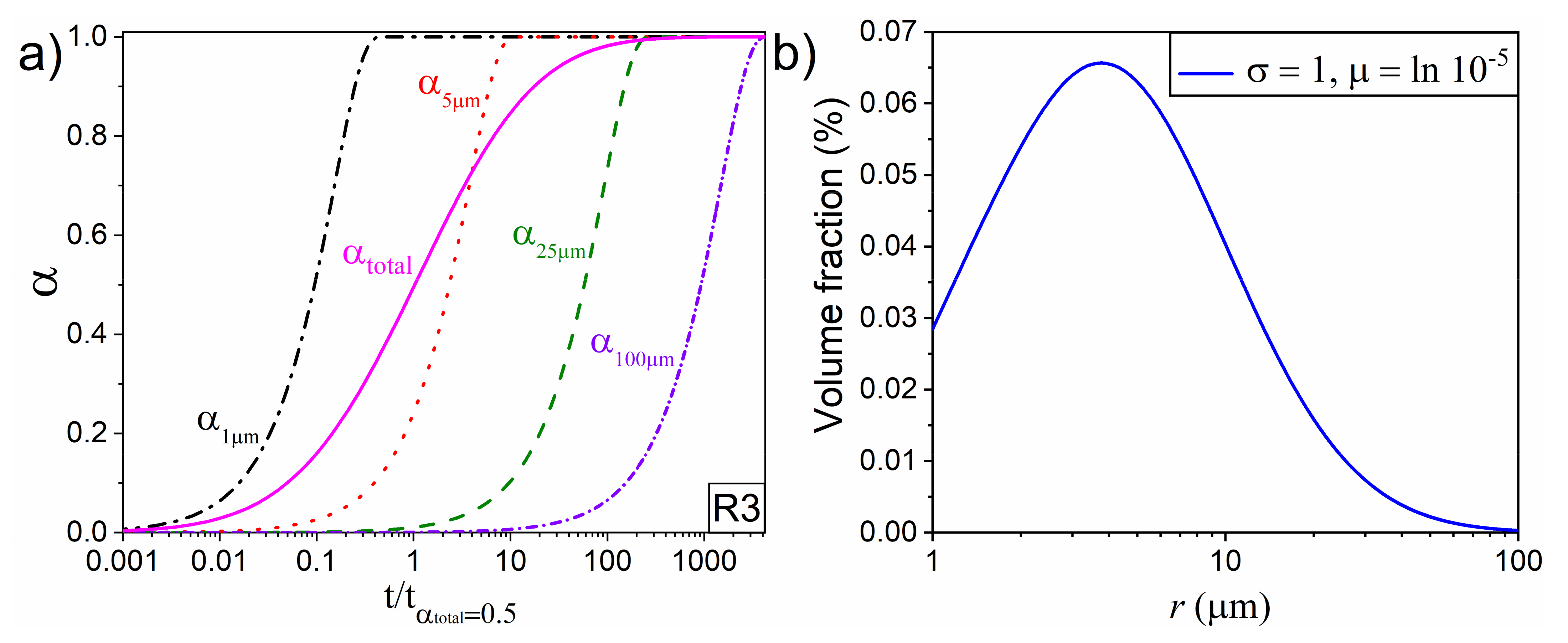
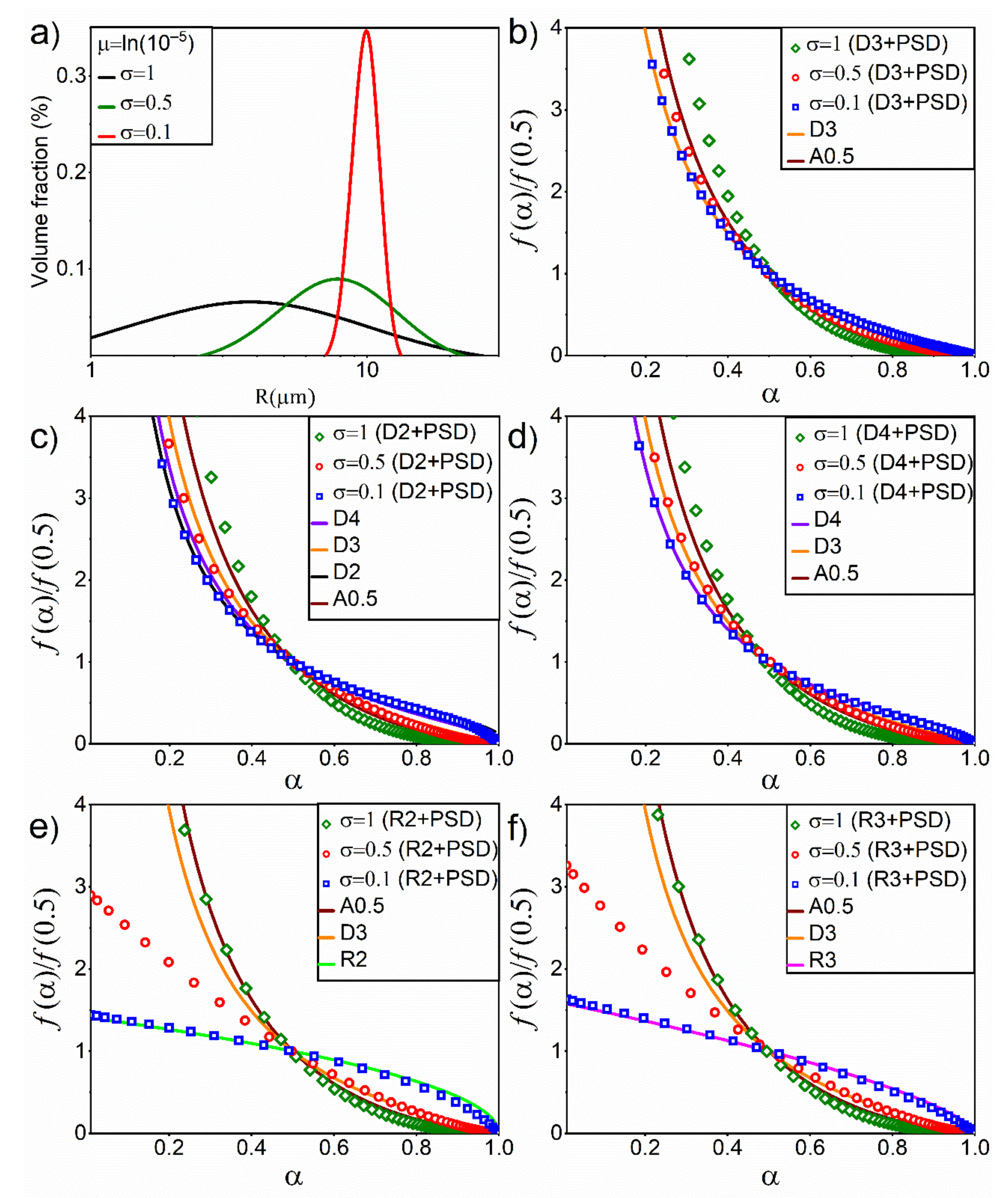
4.1. Effect of PSD in Simulated Linear Heating Experiments

Data plotted in Figure 1a can be used to derive the kinetic model that describes a 3D interface reaction occurring in a sample with the PSD shown in Figure 1b. Indeed, according to Equation (1), this can be achieved by differentiating the curve plotted as the pink solid line as follows:

$$\frac{f\left(\alpha \right)}{f\left(0.5\right)}=\frac{\frac{d\alpha }{dt}}{{\left.\frac{d\alpha }{dt}\right|}_{0.5}}$$

(10)

For the sake of clarity and ease of comparison with other models in the literature, the kinetic model was normalized to its value for $\alpha =$ 0.5. The normalized kinetic model is represented as a function of the extent of the reaction in Figure 2. The ideal model R3 is also plotted in Figure 2. Consistently with the results shown in Figure 1a, the kinetic model is significantly modified when we take PSD into account.

Using the kinetic model plotted in Figure 2, we simulated linear heating experiments intended to study the kinetics of a thermally induced reaction. The results of this simulation are shown in Figure 3a. To simulate the experiments, we solved the following system of equations using the Runge–Kutta method with the initial conditions $T\left(t=0\right)=$ 275 K and $\alpha \left(t=0\right)=$ 10⁻⁴:

$$\begin{gathered} \frac{d\alpha }{dt}=A\exp \left(-\frac{E}{RT}\right)f\left(\alpha \right) \\ \frac{dT}{dt}=\beta \end{gathered}$$

(11)

where $\beta$ represents the heating rates. Four different heating rates were considered: 1, 2, 5, and 10 K·min⁻¹. The pre-exponential factor used was $A=$ 10¹⁰ s⁻¹, and the activation energy was set to $E$ = 100 kJ·mol⁻¹.

Results of the Friedman isoconversional method applied to data in Figure 3a are depicted in Figure 3b. As expected, the values of activation energy remain constant for all the values of conversion. Thus, if this were an analysis of experimental data collected in the laboratory, the conclusions would be that this process can be described with a sole value of activation energy, and there is only one reaction kinetic mechanism [50,51]

To discriminate the kinetic model followed by the process, the combined kinetic analysis, which simultaneously analyzes all experimental data obtained under any heating conditions, was used. This analysis is based on the general kinetic Equation (11) that after rearranging terms can be written in logarithmic form as follows:

$$\ln \left(\frac{\frac{d\alpha }{dt}}{f\left(\alpha \right)}\right)=\ln A-\frac{E}{RT}$$

(12)

Thus, only the correct kinetic model, f($\alpha$), would fit all of the experimental data yielding a straight line from whose slope and intercept the activation energy and preexponential factor can be determined, respectively [52]. Moreover, a modified Sestak–Berggren equation is often used in the simultaneous combined kinetic analysis of experiments conducted under different experimental conditions:

$$f\left(\alpha \right)=C{\left(1-\alpha \right)}^n{\alpha }^m$$

(13)

where $C,n,$ and $m$ are the fitting parameters. The original Sestak–Berggren equation includes a term of the form ${(-\ln \left(1-\alpha \right))}^p$ [53]; however, it has been observed that this modified, simplified version given by Equation (13) can fit every f(α) of the ideal kinetic models most extensively used in the literature [54]. Using this expression, Equation (12) can be rewritten as follows:

$$\ln \left(\frac{d\alpha /dt}{C{\left(1-\alpha \right)}^n{\alpha }^m }\right)=\ln A-\frac{E}{RT}$$

(14)

Therefore, the model that best describes the reaction linearizes $\ln \left(d\alpha /dt/C{\left(1-\alpha \right)}^n{\alpha }^m\right)$ as a function of $1/T$. Thus, the parameters of Equation (13) are obtained by an optimization procedure that yields the parameters that maximize the linear correlation coefficient [54]. Then, the activation energy and the pre-exponential factor are both calculated from the slope and intercept of the plot of $\ln \left(d\alpha /dt/C{\left(1-\alpha \right)}^n{\alpha }^m\right)$ as a function of $1/T$, respectively. Figure 3c shows the results of combined kinetic analysis applied to data presented in Figure 3a. The values of the fitting parameters and correlation coefficient are given in the same graph. The values of $E$ and $A$ obtained are close to those used in the simulation, which validates the use of the combined kinetic analysis in this case. Nonetheless, although Equation (13) can be used to reconstruct the ideal kinetic models accurately with the appropriate choice of values for $C,n,$ and $m$, in general, Equation (13) has no physical meaning for an arbitrary selection of the fitting parameters. A practice commonly employed to provide the obtained equation with a physical significance consists of a graphical comparison with the ideal kinetic models from the literature. This comparison is made in Figure 4. The ideal kinetic models depicted are A0.5, F1, A2, A3 (nucleation), R2, R3 (interface reaction), D2, D3, and D4 (diffusion). Among these models, the one that most resembles the model obtained from the combined kinetic analysis is A0.5, which corresponds to a particular type of Avrami–Erofeev model used to describe a process of nucleation and growth. Therefore, these results lead to the conclusion that the reaction studied follows a nucleation and growth model instead of an interface reaction mechanism modified by the particle size distribution, which is the actual case.

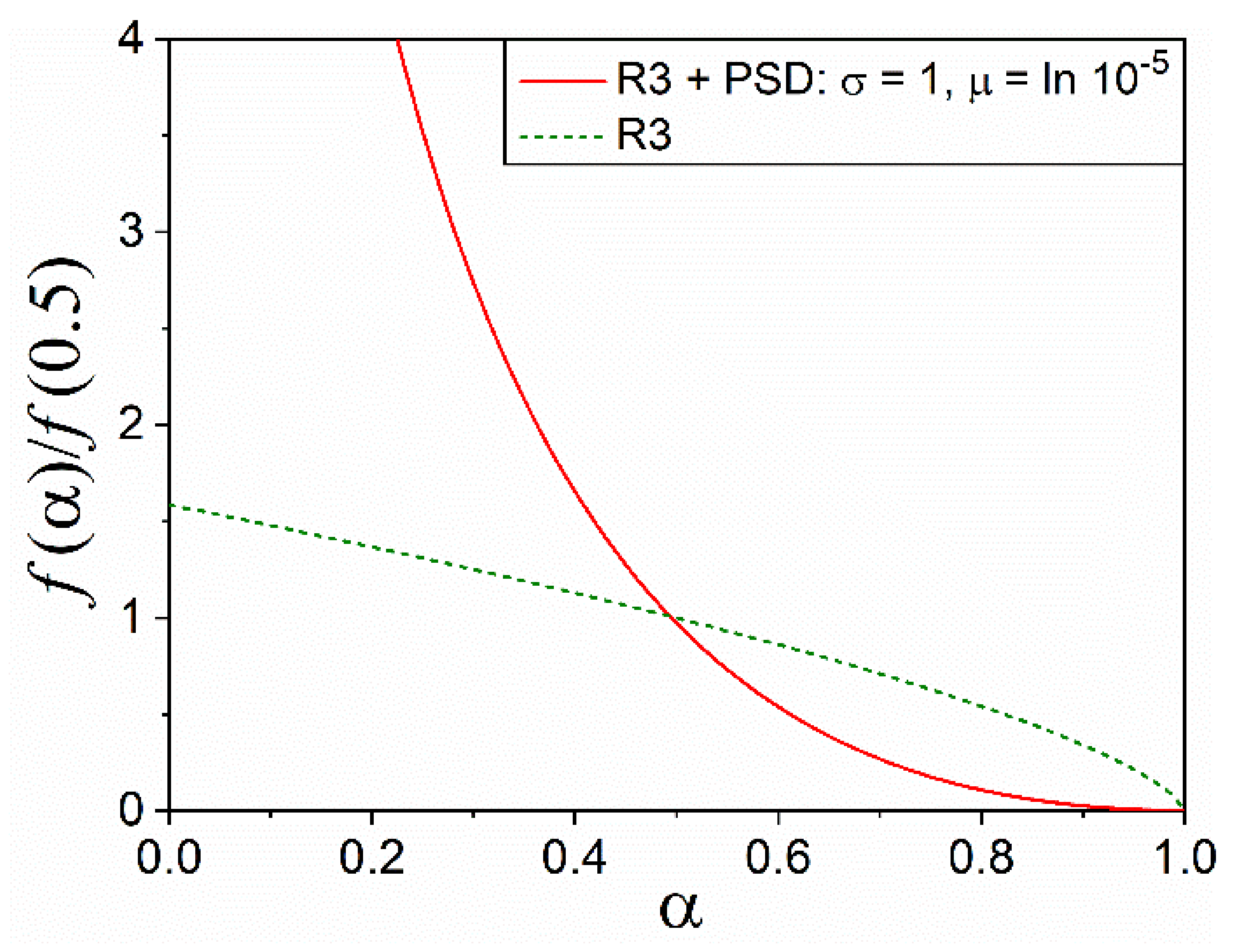
4.2. Effect of PSD on Diffusion and Interface Reaction Models

The study on how PSD modifies the shape of the R3 kinetic model was extended to other ideal models, such as interface growth and diffusion-controlled models (Figure 5 shows the results). In this study, three possible PSDs with $\sigma$ = 0.1, 0.5, and 1, while maintaining $\mu =\ln {10}^{-5}$ constant, were considered in the calculus, (see the resulting PSD curves in Figure 5a). As observed in Figure 5b–d, in the cases of diffusion models, it is hard to discern if the reaction is described by one model or another when PSD comes into play. For instance, a sample with a PSD characterized by $\mu =\ln {10}^{-5}$ and $\sigma =0.5$ that reacts according to D2 could be wrongly assigned to a D3 model (Figure 5c), while D3 can be confused with a nucleation A0.5 model (Figure 5b) when considering PSD.

As observed in Figure 5e,f, the impact seems to be more noticeable in the case of interface reaction models, which can be easily mistaken with a diffusion-type model or a nucleation A0.5 model.

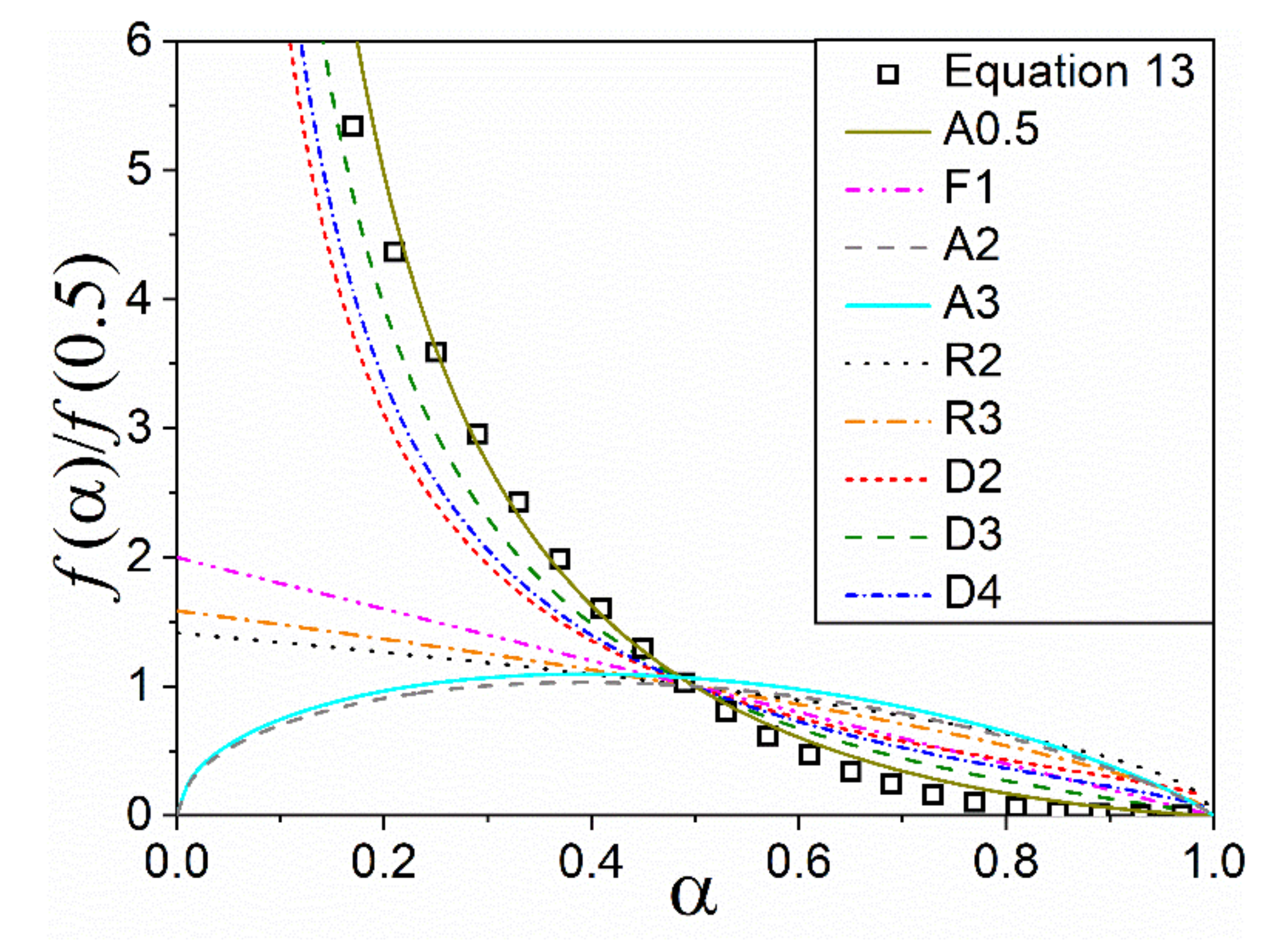
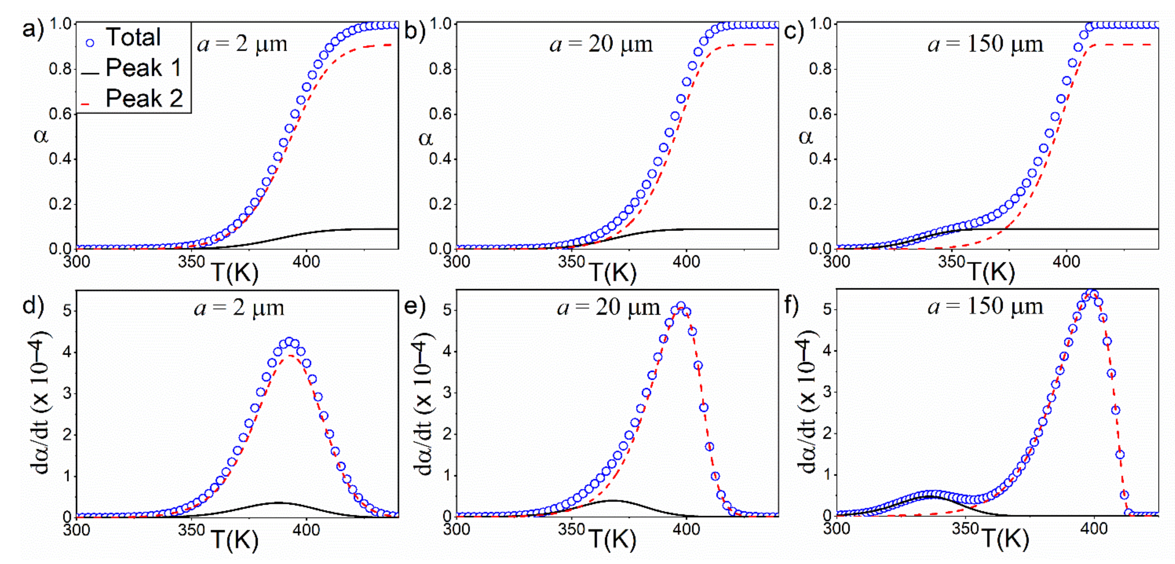
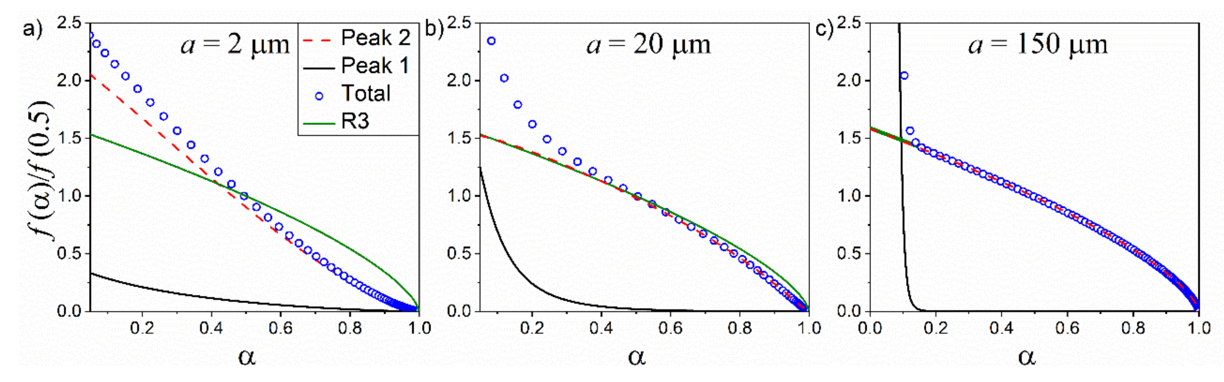
4.3. Effect of a Bimodal PSD in Kinetic Curves

When measuring particle sizes, a PSD that exhibits two separated peaks or humps is commonly found, as observed in the graphs shown in Figure 6. The PSDs shown in this figure was calculated as the sum of two lognormal functions, with $\mu =\ln \left({10}^{-5}\right)$ and $\sigma =0.5$, whose peaks are separated at a variable distance of a. For the sake of clarity, the peaks are plotted separately in each graph as lines, while the sum of both is represented by open blue circles. The calculation was performed assuming that every individual particle in the sample reacts according to the ideal model R3.

The extent of the reaction and its derivative as a function of temperature are plotted in Figure 7. These data were simulated assuming linear heating conditions with a heating rate of $\beta =1$ K·min⁻¹. As in the case of Figure 6, the contribution of each peak is depicted separately as a line, while the total is plotted as open blue circles. As can be observed, the separation between peaks has a clear impact on the shape of the curves $\alpha$-T (Figure 7a–c) and derivatives (Figure 7d–f). For the largest value of a used, the derivative clearly exhibits two humps. This can be explained by the fact that the smaller particles in the left peak of the PSD require much less time to attain a complete reaction than those particles in the right peak of the PSD. Such behavior was observed in Figure 1. Therefore, when the smaller particles complete the reaction, at low values of temperature, a considerable portion of the volume occupied by the larger ones remains unreacted. This result could lead to the misleading conclusion that the reaction is driven by two processes or mechanisms separated by temperature. Therefore, taking PSD into account when performing kinetic analysis is crucial to avoid such mistakes.

Figure 8 shows the kinetic models modified by the consideration of the bimodal PSDs. Again, for the sake of clarity, the contributions of each peak to the kinetic model are presented separately. When a is very large, the kinetic model obtained deviates largely from the ideal one for $\alpha <0.1$, whilst both coincide for higher values of the fractional reaction. As can be observed in Figure 6, the relative relevance of $\sigma$ decreases as a increases, and for a = 150 μm, the second peak can be practically considered as single particle size distribution. This reflects in the graphs of Figure 8, where the contribution of the second peak to $f\left(\alpha \right)$ tends to be the ideal kinetic model used in the simulation (R3) as a increases. For a = 150 μm, the contribution of the second peak and the ideal kinetic model overlap.

As can be inferred from the results shown in Figure 1, for a = 150 μm, only the smaller particles contribute significantly to the reaction rate at the beginning of the reaction, which explains why the contribution of the first peak is much larger in the range of low $\alpha$ values ($\alpha$ < 0.2).

These theoretical results are supported by experimental observations for clay samples of different particle sizes, prepared by a sonication procedure that induces particle size reduction without damaging the crystallographic structure [17,55,56]. These studies show complex TG and DTA profiles, including double peaks, which could be clearly attributed to the contribution of the different particle size fractions to the overall thermal analysis curves rather than to complex thermal mechanisms or intermediate species [57,58].

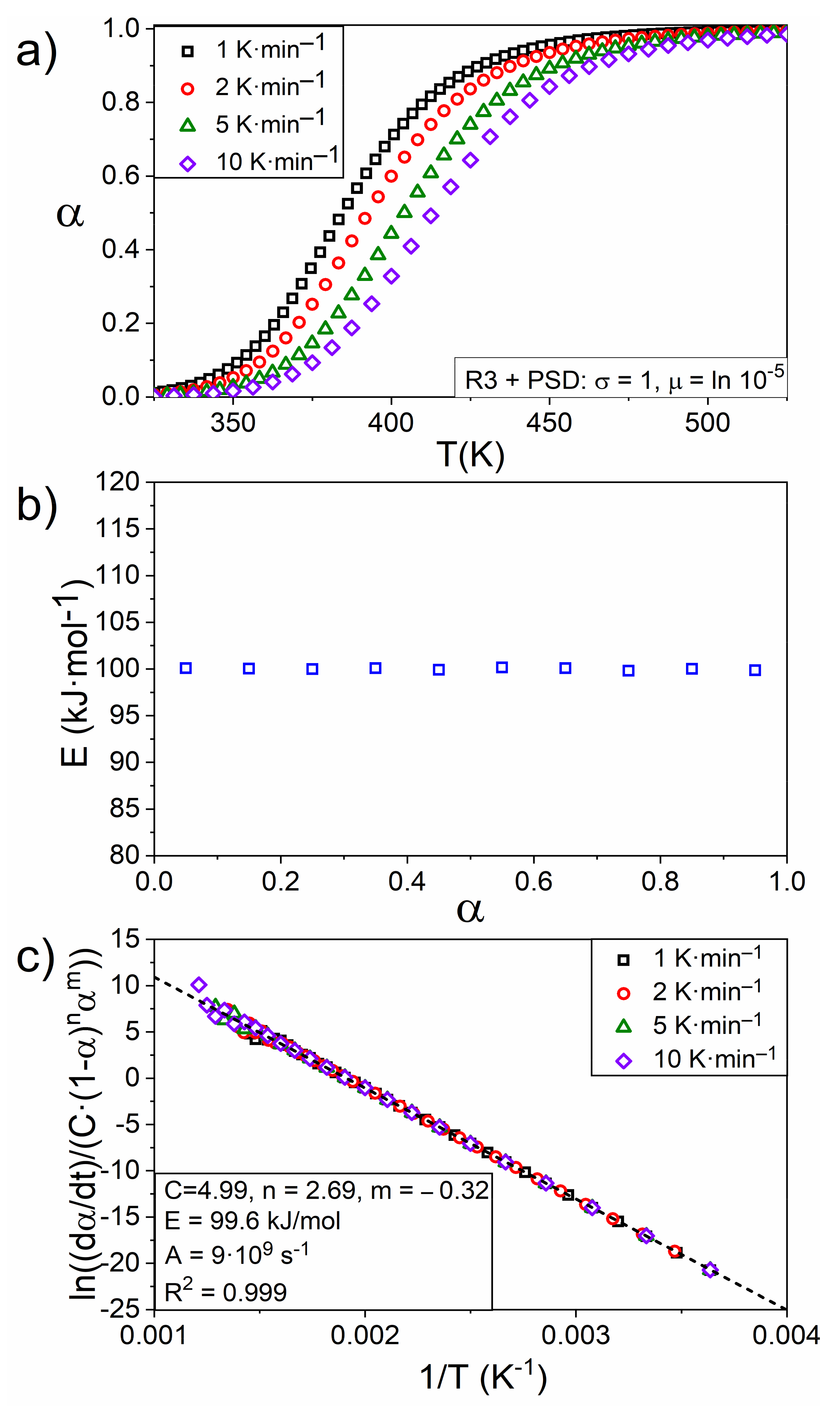
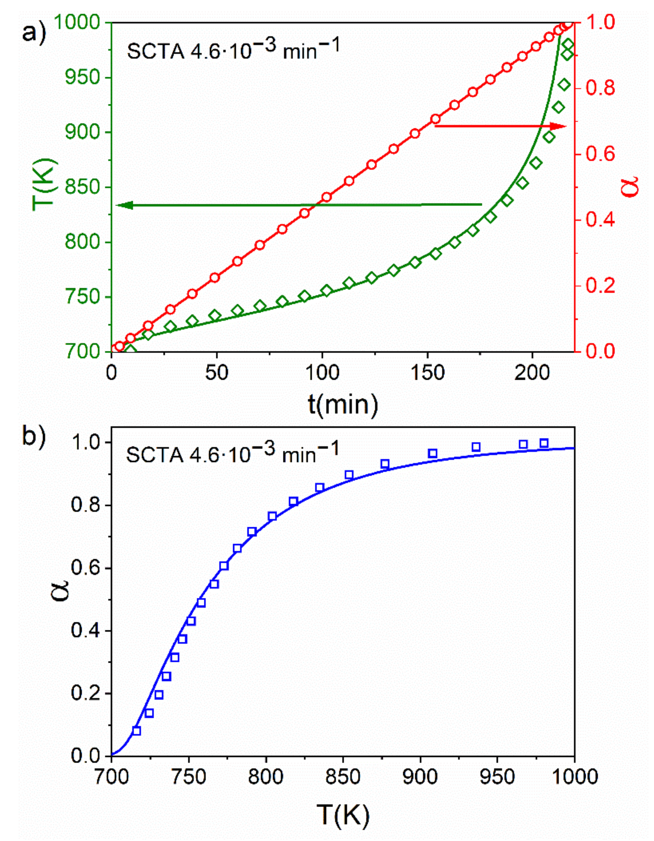
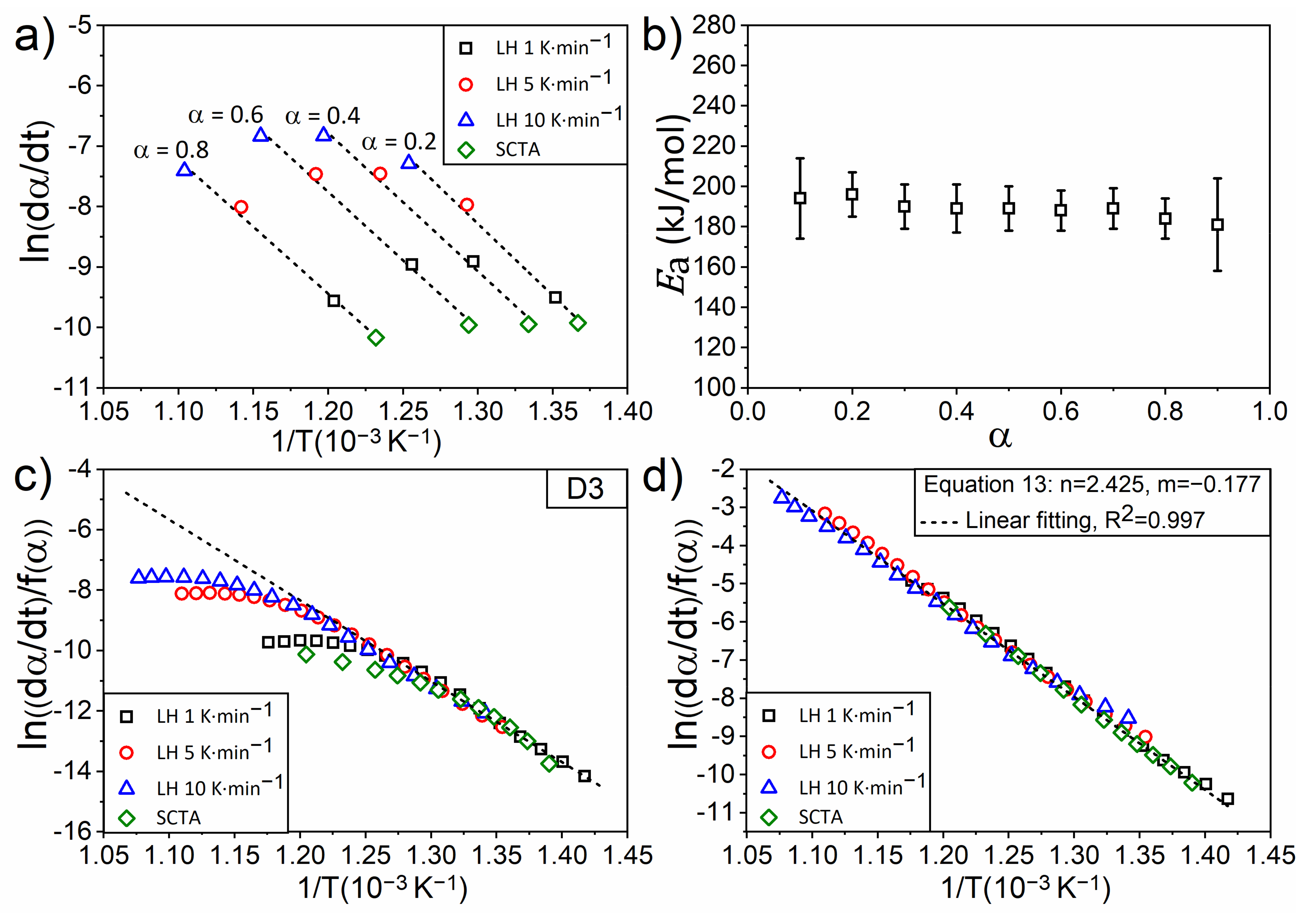
4.4. An Experimental Case: Kinetic of Thermal Dehydroxylation of Kaolinite

Figure 9 shows the values of the extent of the reaction as a function of time in the experiments conducted under linear heating conditions with different heating rates: 1, 5, and 10 K·min⁻¹. The total mass loss of the sample after complete dehydroxylation was in close agreement with the theoretical value ($~$14%).

For the sake of clarity, the experimental data corresponding to the SCTA experiment conducted under the conditions described in the Experimental Section are presented separately in Figure 10. In this experiment, the reaction rate was maintained constant at 4.6·10⁻³ min⁻¹ during the entire experiment, and the relation $\alpha$-time was linear, as observed in Figure 10a. The evolution of temperature with time is also depicted Figure 10a. Additionally, $\alpha$ as a function of temperature is presented in a separate graph (Figure 10b).

Figure 11a,b summarize the results of an isoconversional Friedman analysis to calculate the values of the apparent activation energy during the dehydroxylation process. The results of this analysis indicate that the apparent activation energy remained approximately constant at around (189 $\pm$ 5) kJ/mol during the entire dehydroxylation process (see Figure 11b). This is a common feature of single processes that do not entail a change in mechanism during the process [51,59].

For experimental data shown in Figure 9 and Figure 10, it was observed that all of the most common kinetic models proposed in the literature (F1, A2, A3, R2, R3, D2, and D4) failed at linearizing $\ln \left(\left(d\alpha /dt\right)/f\left(\alpha \right)\right)$ as a function of 1/T (Equation (12)). This indicates that the experimental data could not be fitted by any of these ideal models, despite the fact that the activation energy remains constant in the entire range of $\alpha \mathrm{values}$. Such behavior has been already observed by other authors [29,42,43]. In the case of a D3 model (Figure 11c), which shows the best linearization of all the models, data could be fitted for values of $\alpha <0.6$, but a significant deviation for larger values of $\alpha$ can be observed. Other authors have also observed such a deviation from the ideal model for high values of $\alpha$ and have attributed it to the fact that the metakaolinite formed up to that value of $\alpha$ blocks the interlamellar channels, hindering the escape of water and, thus, curtailing the rate of dehydroxylation [21,60].

By applying the combined kinetic analysis (Equation (14)), it can be observed that the set of experimental data could be linearized in the entire $\alpha$ range for the kinetic model $f\left(\alpha \right)={\alpha }^{-0.177}·{\left(1-\alpha \right)}^{2.425}$, resulting from the optimization process (Figure 11d). Moreover, the value of the apparent activation energy obtained from the slope (E = 191 $\pm$ 1 kJ/mol) is coincident with that obtained by the isoconversional method. Using the resulting kinetic parameters, the experimental curves could be well reconstructed, as shown in Figure 9 and Figure 10. However, the resulting kinetic function does not match any of the ideal kinetic models in the entire range of values for $\alpha$ (Figure 12a). Thus, except for low values of $\alpha$, it fits the D3 kinetic model; for large values, there is a clear deviation from the D3 model, which explains the results in Figure 11c where experimental data could be fitted with a D3 kinetic model only for values of alpha smaller than 0.6, in agreement with previous studies [42,43]. Nevertheless, if the PSD measured experimentally for this sample (Figure 12b) is taken into consideration in the D3 kinetic model, using the same procedure described above for the log normal distribution, the resulting model matches well with the kinetic model resulting in this combined kinetic analysis (Figure 12a). This could be interpreted by considering that kaolinite dehydroxylates according to a D3 model, but the broad particle size distribution plays a significant role in its kinetics in such a way that the time required to achieve a given degree of dehydroxylation depends on the particle size. The non-consideration of PSD leads to discrepancies when comparing the experimental data with the ideal kinetic models. This could be a feasible explanation for the deviation found for the dehydroxylation of kaolinite when interpreted in terms of ideal diffusion models.

5. Conclusions

The influence of PSD on kinetic analysis has been studied both theoretically and experimentally. PSD has a significant effect on the shape of kinetic model functions and might lead to an apparent change in the kinetic mechanism and, therefore, to a misinterpretation of kinetic results. Thus, processes following interface reaction models might look like diffusion-controlled or even nucleation and growth processes, while processes following diffusion-controlled models might look like nucleation and growth processes. Moreover, for bimodal PSD, which is very common in natural samples, complex thermoanalytical profiles are obtained that could be erroneously interpreted in terms of complex reaction mechanisms that involve several stages and intermediate species. Our conclusions are supported experimentally by analyzing the thermal dehydroxylation of kaolinite. This process cannot be fitted by any of the ideal kinetic models despite the fact that the activation energy remains constant throughout the entire range of reaction fractions. We demonstrate that by considering the experimental particle size distribution on an ideal diffusion kinetic model, all experimental curves, obtained under different heating procedures, including linear heating and sample controlled thermal analysis, could be properly fitted.

References

1. Khawam, A.; Flanagan, D.R. Solid-State Kinetic Models: Basics and Mathematical Fundamentals. J. Phys. Chem. B 2006, 110, 17315–17328. [Google Scholar] [CrossRef]
2. Galwey, M.E.; Brown, A.K. Background to Thermal Analysis and Calorimetry, In Handbook of Thermal Analysis and Calorimetry: Applications to Inorganic and Miscellaneous Materials; Elservier Science: Amsterdam, The Netherlands, 1998; Volume 1, p. 147. [Google Scholar]
3. Koga, N.; Tanaka, H. A physico-geometric approach to the kinetics of solid-state reactions as exemplified by the thermal dehydration and decomposition of inorganic solids. Thermochim. Acta 2002, 388, 41–61. [Google Scholar] [CrossRef]
4. Skrdla, P.J. Use of Coupled Rate Equations To Describe Nucleation-and-Branching Rate-Limited Solid-State Processes. J. Phys. Chem. A 2004, 108, 6709–6712. [Google Scholar] [CrossRef]
5. Fedunik-Hofman, L.; Bayon, A.; Donne, S.W. Kinetics of Solid-Gas Reactions and Their Application to Carbonate Looping Systems. Energies 2019, 12, 2981. [Google Scholar] [CrossRef] [Green Version]
6. Frade, J.R.; Cable, M. Reexamination of the Basic Theoretical Model for the Kinetics of Solid-State Reactions. J. Am. Ceram. Soc. 1992, 75, 1949–1957. [Google Scholar] [CrossRef]
7. Cooper, E.A.; Mason, T.O. Mechanism of La2CuO4 Solid-State Powder Reaction by Quantitative XRD and Impedance Spectroscopy. J. Am. Ceram. Soc. 1995, 78, 857–864. [Google Scholar] [CrossRef]
8. Sasaki, H. Introduction of Particle-Size Distribution into Kinetics of Solid-State Reaction. J. Am. Ceram. Soc. 1964, 47, 512–516. [Google Scholar] [CrossRef]
9. Kapur, P.C. Kinetics of Solid-State Reactions of Particulate Ensembles with Size Distributions. J. Am. Ceram. Soc. 1973, 56, 79–81. [Google Scholar] [CrossRef]
10. Miyagi, S. Criticism on Jander’s Equation of Reaction-Rate, Considering Statistical Distribution of Particle Size of Reacting Substance. J. Ceram. Assoc. Jpn. 1951, 59, 132–135. [Google Scholar] [CrossRef] [Green Version]
11. Koga, N.; Criado, J.M. Kinetic Analyses of Solid-State Reactions with a Particle-Size Distribution. J. Am. Ceram. Soc. 1998, 81, 2901–2909. [Google Scholar] [CrossRef]
12. Urrutia, G.A.; Blesa, M.A. The influence of particle size distribution on the conversion/time profiles under contracting-geometry kinetic regimes. React. Solids 1988, 6, 281–284. [Google Scholar] [CrossRef]
13. HMurray, H.H. Traditional and new applications for kaolin, smectite, and palygorskite: A general overview. Appl. Clay Sci. 2000, 17, 207–221. [Google Scholar] [CrossRef]
14. Massaro, M.; Colletti, C.G.; Lazzara, G.; Riela, S. The Use of Some Clay Minerals as Natural Resources for Drug Carrier Applications. J. Funct. Biomater. 2018, 9, 58. [Google Scholar] [CrossRef] [Green Version]
15. ERuiz-Hitzky, E.; Aranda, P.; Darder, M. Hybrid and Biohybrid Materials Based on Layered Clays. In Tailored Organic-Inorganic Materials, 1st ed.; Brunet, E., Colón, J.L., Clearfield, A., Eds.; Instituto de Ciencia de Materiales de Madrid, ICMM-CSIC Cantoblanco: Madrid, Spain, 2015; pp. 245–297. [Google Scholar] [CrossRef]
16. Zhao, B.; Liu, L.; Cheng, H. Rational design of kaolinite-based photocatalytic materials for environment decontamination. Appl. Clay Sci. 2021, 208, 106098. [Google Scholar] [CrossRef]
17. Franco, F.; Pérez-Maqueda, L.; Pérez-Rodríguez, J. The effect of ultrasound on the particle size and structural disorder of a well-ordered kaolinite. J. Colloid Interface Sci. 2004, 274, 107–117. [Google Scholar] [CrossRef]
18. Belviso, C.; Cavalcante, F.; Lettino, A.; Fiore, S. A and X-type zeolites synthesised from kaolinite at low temperature. Appl. Clay Sci. 2013, 80–81, 162–168. [Google Scholar] [CrossRef]
19. Rashad, A.M. Metakaolin as cementitious material: History, scours, production and composition—A comprehensive overview. Constr. Build. Mater. 2013, 41, 303–318. [Google Scholar] [CrossRef]
20. Nawaz, M.; Heitor, A.; Sivakumar, M. Geopolymers in construction—Recent developments. Constr. Build. Mater. 2020, 260, 120472. [Google Scholar] [CrossRef]
21. Criado, J.M.; Ortega, A.; Real, C.; De Torres, E.T. Re-examination of the kinetics of the thermal dehydroxylation of kaolinite. Clay Miner. 1984, 19, 653–661. [Google Scholar] [CrossRef]
22. Bellotto, M.; Gualtieri, A.; Artioli, G.; Clark, S.M. Kinetic study of the kaolinite-mullite reaction sequence. Part I: Kaolinite dehydroxylation. Phys. Chem. Miner. 1995, 22, 207–217. [Google Scholar] [CrossRef]
23. Redfern, S.A.T. The kinetics of dehydroxylation of kaolinite. Clay Miner. 1987, 22, 447–456. [Google Scholar] [CrossRef]
24. Gasparini, E.; Tarantino, S.; Ghigna, P.; Riccardi, M.P.; Cedillo-González, E.I.; Siligardi, C.; Zema, M. Thermal dehydroxylation of kaolinite under isothermal conditions. Appl. Clay Sci. 2013, 80–81, 417–425. [Google Scholar] [CrossRef]
25. Ortega, A.; Gotor, F.J.; Macías, M. The Multistep Nature of the Kaolinite Dehydroxylation: Kinetics and Mechanism. J. Am. Ceram. Soc. 2010, 93, 197–203. [Google Scholar] [CrossRef]
26. Murray, P.; White, J. Kinetics of the Thermal Dehydration of Clays. Trans. Br. Ceram. Soc. 1955, 54, 137–150. [Google Scholar]
27. Frost, R.L.; Vassallo, A.M. The Dehydroxylation of the Kaolinite Clay Minerals using Infrared Emission Spectroscopy. Clays Clay Miner. 1996, 44, 635–651. [Google Scholar] [CrossRef]
28. Ortega, A.; Rouquérol, F.; Akhouayri, S.; Laureiro, Y.; Rouquerol, J. Kinetical study of the thermolysis of kaolinite between −30° and 1000 °C by controlled rate evolved gas analysis. Appl. Clay Sci. 1993, 8, 207–214. [Google Scholar] [CrossRef]
29. Liu, X.; Liu, X.; Hu, Y. Investigation of the thermal behaviour and decomposition kinetics of kaolinite. Clay Miner. 2015, 50, 199–209. [Google Scholar] [CrossRef]
30. Ptáček, P.; Frajkorová, F.; Soukal, F.; Opravil, T. Kinetics and mechanism of three stages of thermal transformation of kaolinite to metakaolinite. Powder Technol. 2014, 264, 439–445. [Google Scholar] [CrossRef]
31. Ptáček, P.; Soukal, F.; Opravil, T.; Havlica, J.; Brandštetr, J. The kinetic analysis of the thermal decomposition of kaolinite by DTG technique. Powder Technol. 2011, 208, 20–25. [Google Scholar] [CrossRef]
32. KNahdi, K.; Llewellyn, P.; Rouquérol, F.; Ariguib, N.; Ayedi, M. Controlled Rate Thermal Analysis of kaolinite dehydroxylation: Effect of water vapour pressure on the mechanism. Thermochim. Acta 2002, 390, 123–132. [Google Scholar] [CrossRef]
33. Allison, E.B. The dtermination of specific heats of reaction of clay minerals by thermal analysis. Silic. Ind. 1954, 19, 363–373. [Google Scholar]
34. Cabrera, J.; Eddleston, M. Kinetics of dehydroxylation and evaluation of the crystallinity of kaolinite. Thermochim. Acta 1983, 70, 237–247. [Google Scholar] [CrossRef]
35. Ondro, T.; Húlan, T.; Vitázek, I. Non-Isothermal Kinetic Analysis of the Dehydroxylation of Kaolinite in Dynamic Air Atmosphere. Acta Technol. Agric. 2017, 20, 52–56. [Google Scholar] [CrossRef] [Green Version]
36. Saikia, D.N.; Sengupta, P.; Gogoi, P.; Borthakur, P.C. Kinetics of dehydroxylation of kaolin in presence of oil field effluent treatment plant sludge. Appl. Clay Sci. 2002, 22, 93–102. [Google Scholar] [CrossRef]
37. Levy, J.H.; Hurst, H. Kinetics of dehydroxylation, in nitrogen and water vapour, of kaolinite and smectite from Australian Tertiary oil shale. Fuel 1993, 72, 873–877. [Google Scholar] [CrossRef]
38. Ptáček, P.; Kubátová, D.; Havlica, J.; Brandštetr, J.; Soukal, F.; Opravil, T. The non-isothermal kinetic analysis of the thermal decomposition of kaolinite by thermogravimetric analysis. Powder Technol. 2010, 204, 222–227. [Google Scholar] [CrossRef]
39. Brindley, G.W.; Sharp, J.H.; Patterson, J.H.; Narahari, B.N. Kinetics and Mechanism of Dehydroxylation Processes, I. Temperature and Vapor Pressure Dependence of Dehydroxylation of Kaolinite. Am. Mineral. 1967, 52, 201–211. [Google Scholar]
40. Redaoui, D.; Sahnoune, F.; Heraiz, M.; Belhouchet, H.; Fatmi, M. Thermal decomposition kinetics of Algerian Tamazarte kaolinite by thermogravimetric analysis. Trans. Nonferrous Met. Soc. China 2017, 27, 1849–1855. [Google Scholar] [CrossRef]
41. Horváth, I. Kinetics and compensation effect in kaolinite dehydroxylation. Thermochim. Acta 1985, 85, 193–198. [Google Scholar] [CrossRef]
42. Dion, P.; Alcover, J.-F.; Bergaya, F.; Ortega, A.; Llewellyn, P.L.; Rouquérol, F. Kinetic study by controlled-transformation rate thermal analysis of the dehydroxylation of kaolinite. Clay Miner. 1998, 33, 269–276. [Google Scholar] [CrossRef]
43. Zhang, X.L.Z.; Zhong, Y.; Wang, L.; Liao, G.; Wang, R.; Li, Z.; Li, J. Kinetic analysis of non-isothermal dehydroxylation of kaolinite based on isoconversional and multivariate non-linear regression methods. Kuangwu Yanshi 2019, 39, 1–7. [Google Scholar] [CrossRef]
44. Pérez-Maqueda, L.; Sanchez, P.; Criado, J. Evaluation of the integral methods for the kinetic study of thermally stimulated processes in polymer science. Polymer 2005, 46, 2950–2954. [Google Scholar] [CrossRef] [Green Version]
45. Perez-Rodriguez, J.L.; Duran, A.; Jiménez, P.E.S.; Franquelo, M.L.; Perejón, A.; Pascual-Cosp, J.; Pérez-Maqueda, L.A. Study of the Dehydroxylation-Rehydroxylation of Pyrophyllite. J. Am. Ceram. Soc. 2010, 93, 2392–2398. [Google Scholar] [CrossRef] [Green Version]
46. Rouquerol, J. Thermal analysis: Sample-controlled techniques. In Encyclopedia of Analytical Science; Elsevier: Amsterdam, The Netherlands, 2019; pp. 17–321. [Google Scholar]
47. Pérez-Maqueda, L.A.; Ortega, A.; Criado, J.M. The use of master plots for discriminating the kinetic model of solid state reactions from a single constant-rate thermal analysis (CRTA) experiment. Thermochim. Acta 1996, 277, 165–173. [Google Scholar] [CrossRef]
48. Chopra, G.S.; Real, C.; Alcalá, M.D.; Perez-Maqueda, L.A.; Subrt, J.; Criado, J.M. Factors Influencing the Texture and Stability of Maghemite Obtained from the Thermal Decomposition of Lepidocrocite. Chem. Mater. 1999, 11, 1128–1137. [Google Scholar] [CrossRef]
49. Pérez-Maqueda, L.A.; Criado, J.M.; Real, C.; Šubrt, J.; Boháček, J. The use of constant rate thermal analysis (CRTA) for controlling the texture of hematite obtained from the thermal decomposition of goethite. J. Mater. Chem. 1999, 9, 1839–1846. [Google Scholar] [CrossRef]
50. Pérez-Maqueda, L.A.; Sánchez-Jiménez, P.E.; Criado, J.M. Kinetic analysis of solid-state reactions: Precision of the activation energy calculated by integral methods. Int. J. Chem. Kinet. 2005, 37, 658–666. [Google Scholar] [CrossRef] [Green Version]
51. Vyazovkin, S.; Burnham, A.K.; Favergeon, L.; Koga, N.; Moukhina, E.; Pérez-Maqueda, L.A.; Sbirrazzuoli, N. ICTAC Kinetics Committee recommendations for analysis of multi-step kinetics. Thermochim. Acta 2020, 689, 178597. [Google Scholar] [CrossRef]
52. Pérez-Maqueda, L.A.; Criado, J.M.; Gotor, F.J.; Málek, J. Advantages of Combined Kinetic Analysis of Experimental Data Obtained under Any Heating Profile. J. Phys. Chem. A 2002, 106, 2862–2868. [Google Scholar] [CrossRef]
53. Šesták, J.; Berggren, G. Study of the kinetics of the mechanism of solid-state reactions at increasing temperatures. Thermochim. Acta 1971, 3, 1–12. [Google Scholar] [CrossRef]
54. Pérez-Maqueda, L.A.; Criado, A.J.M.; Sánchez-Jiménez, P.E. Combined Kinetic Analysis of Solid-State Reactions: A Powerful Tool for the Simultaneous Determination of Kinetic Parameters and the Kinetic Model without Previous Assumptions on the Reaction Mechanism. J. Phys. Chem. A 2006, 110, 12456–12462. [Google Scholar] [CrossRef]
55. Franco, F.; Cecila, J.; Pérez-Maqueda, L.; Pérez-Rodríguez, J.; Gomes, C. Particle-size reduction of dickite by ultrasound treatments: Effect on the structure, shape and particle-size distribution. Appl. Clay Sci. 2007, 35, 119–127. [Google Scholar] [CrossRef]
56. Wiewióra, A.; Pérez-Rodrıguez, J.L.; Perez-Maqueda, L.A.; Drapała, J. Particle size distribution in sonicated high- and low-charge vermiculites. Appl. Clay Sci. 2003, 24, 51–58. [Google Scholar] [CrossRef]
57. Perez-Maqueda, L.A.; Blanes, J.M.M.; Pascual, J.; Pérez-Rodríguez, J.L. The influence of sonication on the thermal behavior of muscovite and biotite. J. Eur. Ceram. Soc. 2004, 24, 2793–2801. [Google Scholar] [CrossRef]
58. Pérez-Maqueda, L.A.; Montes, O.M.; González-Macias, E.M.; Franco, F.; Poyato, J.; Pérez-Rodrıguez, J.L. Thermal transformations of sonicated pyrophyllite. Appl. Clay Sci. 2004, 24, 201–207. [Google Scholar] [CrossRef]
59. Vyazovkin, S.; Burnham, A.; Criado, J.M.; Perez-Maqueda, L.A.; Popescu, C.; Sbirrazzuoli, N. ICTAC Kinetics Committee recommendations for performing kinetic computations on thermal analysis data. Thermochim. Acta 2011, 520, 1–19. [Google Scholar] [CrossRef]
60. Otero-Arean, C.; Letellier, M.; Gerstein, B.C.; Fripiat, J.J. Protonic structure on kaolinite during dehydroxylation studied by proton nuclear magnetic resonance. Summary 1982, 105, 499. [Google Scholar] [CrossRef]
Figure 1. (a) Fractional reaction as a function of normalized time for different particle sizes. The overall values for the sample are plotted as a pink solid line. (b) Lognormal PSD with σ = 1 and μ = ln 10 5 .
Processes 09 01852 g001
Figure 2. Normalized kinetic models. The dashed green line represents the ideal model R3, whilst the continuous red line corresponds to the kinetic model obtained when PSD is taken into account.
Processes 09 01852 g002
Figure 3. (a) Curves simulated under linear heating conditions using the kinetic model R3 with the PSD shown in Figure 1b. (b) Values of activation energy as a function of the fractional reaction obtained by the Friedman isoconversional method. (c) Combined kinetic analysis.
Processes 09 01852 g003
Figure 4. Comparison between the modified Sestak–Berggren equation obtained from combined analysis (open black squares) and some ideal kinetic models from the literature (lines) [1].
Processes 09 01852 g004
Figure 5. Modification of ideal kinetic models when PSD is taken into consideration. (a) Different PSD used. (b) D3, (c) D2, (d) D4, (e) R2 and (f) R3.
Processes 09 01852 g005
Figure 6. Bimodal particle size distributions using the simulations. The total PSD was calculated as the sum of two lognormal functions, with μ = ln 10 5 and σ = 0.5 being the amplitude of the second peak ten times the amplitude of the first one. The separation between peaks was set at (a) 2 μm, (b) 20 μm, and (c) 150 μm.
Processes 09 01852 g006
Figure 7. (ac) Curves of α as a function of temperature, simulated using the R3 kinetic models modified by bimodal PSD, with β = 1 K·min−1 and a = 2, 20 and 150 μm, respectively. (df) Derivative of α with time as a function of temperature for a = 2, 20 and 150 μm, respectively.
Processes 09 01852 g007
Figure 8. Kinetic models modified by the consideration of the bimodal PSDs. The curves that represent the contribution of the peaks are plotted as lines, while the total kinetic model is depicted as a set of blue open circles. The separation between the two peaks of the bimodal PSDs was set at (a) 2 μm, (b) 20 μm and (c) 150 μm.
Processes 09 01852 g008
Figure 9. Reacted fraction as a function of temperature in the experiments conducted under linear heating conditions: 1, 5, and 10 K·min1. Experimental data are depicted as open symbols. Solid lines represent the curves reconstructed using the modified Sestak–Berggren equation (Equation (13)), where n = 2.425 and m = −0.177.
Processes 09 01852 g009
Figure 10. Dehydroxylation of kaolinite conducted under SCTA (4.6·10−3 min−1). (a) Time evolution of the reacted fraction and temperature during reaction. (b) Reacted fraction as a function of temperature. Experimental data are depicted as open symbols. Solid lines represent the curves reconstructed using the kinetic parameters resulting from the analysis.
Processes 09 01852 g010
Figure 11. (a) ln d α / d t as a function of the inverse of temperature 1/T for different values of α . (b) Values of the apparent activation energy as obtained by the Friedman isoconversional analysis (Figure 11a) as a function of α . (c) ln d α / d t / f α as a function of the inverse of temperature 1/T for D3 and (d) for the modified Sestak–Berggren equation (Equation (13)) with the n and m parameters resulting from the optimization procedure.
Processes 09 01852 g011
Figure 12. (a) Comparison between the Sestak–Berggren model obtained for the dehydroxilation of kaolinite, represented as open symbols, and some ideal kinetic models from the literature. The D3 kinetic model, modified considering the PSD is also included as a red solid line. (b) PSD of the kaolinite sample used in this work.
Processes 09 01852 g012