Synthesis of Polynomial Fuzzy Model-Based Designs with Synchronization and Secure Communications for Chaos Systems with H_∞ Performance

Abstract

This paper presents the sum of squares (SOS)-based fuzzy control with H∞ performance for a synchronized chaos system and secure communications. To diminish the influence of the extrinsic perturbation, SOS-based stability criteria of the polynomial fuzzy system are derived by using the polynomial Lyapunov function. The perturbation decreasing achievement is indexed in a H∞ criterion. The submitted SOS-based stability criteria are more relaxed than the existing linear matrix inequality (LMI)-based stability criteria. The cryptography scheme based on an n-shift cipher is combined with synchronization for secure communications. Finally, numerical simulations illustrate the perturbation decay accomplishment of the submitted polynomial fuzzy compensator.

1. Introduction

In recent years, the studies on synchronization of chaos systems have acquired substantial attention. The drive-response frame, which is the means to synchronize chaos systems, was established by Caroll and Pecora [1]. The master chaos system, as a drive system, is synchronized with another chaos system, the response system. Complicated dynamic phenomena are the major characteristics of chaos systems. For instance, chaos systems are sensitive to parameter variation and initial conditions, such that the trajectory of states is unpredictable. As a result of these properties, chaos synchronization can be applied to communications for security and privacy [2], and photovoltaic module fault detection [3]. How to operate the variables of the response system to equal those of the drive system in various original states is the essential problem of the synchronization of chaos systems.

Many control methods have been developed for chaos synchronization, such as iterative learning control [4], robust adaptive control [5], sliding mode control [6], and adaptive fuzzy perturbation observer [7]. The Takagi–Sugeno (T-S) fuzzy model with linear matrix inequality (LMI) control is effective among these control strategies. A nonlinear dynamic plant can be easily described by using the T-S fuzzy model, which is constructed from IF–THEN fuzzy rules [8]. By using the parallel distributed compensation (PDC) method, T-S fuzzy compensators can be portrayed. Furthermore, solving LMI-based stability conditions can secure the state feedback gain. Thus, chaotic systems have been synchronized through T-S fuzzy modeling and control [9,10,11,12]. In [9], the LMI-based fuzzy control was applied to synchronization of chaotic systems. In [10], the perturbation observer-based LMI was engaged for the synchronization of T-S fuzzy chaos systems. In [11], the design of an adaptive TSK fuzzy self-organizing compensator was proposed for chaotic systems. An exact linearization (EL) technique, which was employed to synchronize the chaotic systems via the PDC, has been discussed [12]. However, there still exist two design issues in LMI-based T-S fuzzy control methodology. First, T-S fuzzy models cannot describe all nonlinear systems. Second, the LMI-based stability conditions will be very tentative if the quadratic Lyapunov function is employed. Thus, some literature has taken relaxed stability conditions into account [13,14,15]. In [13], the conservativeness of stabilization criterion for the T-S fuzzy system was significantly relaxed using the constraints condition of the controller membership functions. From a line-integral Lyapunov function, a possible conservatism generated by the derivation of the membership function was removed to raise the relaxation of the sufficient conditions [14]. In [15], the piecewise fuzzy Lyapunov function was introduced and less conservatism was attained. Therefore, this paper employs a polynomial Lyapunov function to acquire the sum of squares (SOS)-based stability criteria of chaotic synchronization systems to reduce the conservativeness of the LMI-based stability criteria.

The polynomial fuzzy model can more efficaciously characterize the nonlinear system than the T-S fuzzy model [16]. Several studies on polynomial fuzzy control systems have been investigated recently [17,18,19,20,21]. In [17], polynomial Lyapunov functions are designed by introducing a gradient algorithm without applying the typical transformation so that the polynomial fuzzy controller with SOS stability conditions was received. In [18], the message and character of membership functions are deliberated in the SOS-based stability design of (interval type 2) IT2 polynomial-fuzzy-model-based control systems. In [19], a homogeneously state-dependent polynomial Lyapunov function was proposed for an observed-state feedback polynomial fuzzy control system. In [20], using a free full-block multiplier, the conservativeness of SOS-based stability analysis was reduced. In [21], using the Lyapunov function and the S-procedure, SOS-based stability criteria are received for uncertain large-scale polynomial T–S fuzzy systems. However, when an extrinsic perturbation occurs in the chaos synchronization systems, the stability of the system cannot be guaranteed using these SOS criteria.

Consequently, based on the above observations from the literature, this paper takes extrinsic perturbation into account to synthesize the $H_{\infty }$ control of polynomial fuzzy chaos synchronization systems. That is, the proffered SOS-based stability conditions not only guarantee that the chaos synchronization systems are stable but also that $H_{\infty }$ is achieved for the perturbation attenuation. Further, the proffered methodology can evade the aforesaid shortcomings of the T-S fuzzy compensator with LMI stability criteria. Moreover, the cryptography scheme based on an n-shift cipher combined with synchronization is applied to increase the security of the transmitted signal. The solutions of the submitted SOS-based criteria in this paper were determined by using SOSTOOLS [22]. This paper proposes two novel theorems and the contributions of this article are summarized as follows. First, SOS-based stability criteria with $H_{\infty }$ performance are proposed for chaos synchronization. Then, a second theorem with SOS stability criteria is acquired to perform quasi-linearization (QL) of a chaos system.

This paper is organized as follows. In Section 2.1, the polynomial fuzzy systems with extrinsic perturbation are given. Moreover, using the polynomial Lyapunov function, we derive the SOS stability criteria and obtain $H_{\infty }$. In Section 2.2 and Section 2.3, the chaos synchronization and secure communication are discussed. Section 3 shows the simulation results of the comparison with the SOS approach and the LMI approach. Finally, some conclusions are drawn in Section 4.

2. Methods

This section presents the design of a polynomial fuzzy compensator for synchronized chaos systems and secure communications. First, stability criteria are derived for the polynomial fuzzy system with extrinsic perturbation. Second, the drive-response structure is employed for chaotic synchronization, and two cases of the polynomial fuzzy synchronized chaos system are studied. Last, the polynomial fuzzy synchronized chaos system is combined with cryptography technology to raise the security of communications.

2.1. $H_{\infty }$ Polynomial Fuzzy Compensator

The extrinsic perturbation in chaos synchronization systems will result in destroying stability or degrading accomplishment. The polynomial fuzzy model can more efficaciously characterize the nonlinear system and is more universal than the Takagi-Sugeno (T-S) fuzzy model. Accordingly, the $H_{\infty }$ polynomial fuzzy control will be investigated for chaos systems in this section.

2.1.1. Polynomial Fuzzy Chaos System with Extrinsic Perturbation

The state variables are included in the polynomial fuzzy chaos system with extrinsic perturbation. The following fuzzy rules describe the polynomial fuzzy chaos system.

$$\begin{gathered} \mathit{IF}{z}_1(t)\mathrm{is}{M}_{i1}\dots \dots \mathrm{and}{z}_p(t)\mathrm{is}{M}_{ip} \\ \mathit{THEN}\dot{x}(t)=A_i(x(t))\widehat{x}(x(t))+Bu(t)+Dn(t) \\ y(t)=C\widehat{x}(x(t))\hspace{1em}\hspace{1em}\hspace{1em}\hspace{1em}\hspace{1em}\hspace{1em}\hspace{1em}i=1,2,\dots ,r. \end{gathered}$$

(1)

where $z(t)=[z_1(t),z_2(t),\cdots ,z_P(t)]$ denotes the variables in the premise, $M_{ij}(j=1,2,\dots ,p)$ is the membership function, and r indicates the number of fuzzy rules. $x\left(t\right)\in R^n$ denotes a state vector. $\widehat{x}(x(t))\in R^N$ is a vector of which all elements are monomials in $x\left(t\right)$. $A_i(x(t))\in R^{n\times N}$ indicates a polynomial system matrix. $B\in R^{n\times m}$, $D\in R^{n\times p}$, and $C\in R^{q\times N}$ denote constant system matrices. $u(t)\in R^m$ is a compensator input. $n(t)\in R^p$ indicates a perturbation. $y(t)\in R^q$ denotes a vector of output signal.

The results of the polynomial fuzzy chaos plant are expressed by

$$\begin{gathered} \dot{x}(t)=\frac{{\displaystyle \sum _{i=1}^r{\omega }_i(z(t))\{A_i(x(t))\widehat{x}(x(t))+Bu(t)+Dn(t)\}}}{{\displaystyle \sum _{i=1}^r{\omega }_i(z(t))}} \\ ={\displaystyle \sum _{i=1}^r{h}_i(z(t))\{A_i(x(t))\widehat{x}(x(t))+Bu(t)+Dn(t)\}} \\ y(t)=C\widehat{x}(x(t)) \end{gathered}$$

(2)

where

$${\omega }_i(z(t))={\displaystyle \prod _{j=1}^P{M}_{ij}(z_j(t))},{\omega }_i(z(t))\ge 0,{\displaystyle \sum _{i=1}^r{\omega }_i(z(t))}>0,i=1,2,\dots ,r.$$

(3)

Thus,

$$h_i(z(t))=\frac{{\omega }_i(z(t))}{{\displaystyle \sum _{i=1}^r{\omega }_i(z(t))}},\hspace{1em}\hspace{1em}\hspace{1em}\hspace{1em}{\displaystyle \sum _{i=1}^r{h}_i(z(t))}=1$$

(4)

2.1.2. Polynomial Fuzzy Compensator Gain

Based on the parallel distributed compensation (PDC) strategy, both the polynomial fuzzy compensator and the polynomial fuzzy model have identical fuzzy membership functions. The polynomial fuzzy compensator can hold state variables, which is the principal discrimination between the polynomial fuzzy compensator and the T-S fuzzy compensator. The following presents the fuzzy control if–then rules

$$\begin{gathered} \mathit{IF}{z}_1(t)\mathrm{is}{M}_{i1}\dots \dots \mathrm{and}{z}_p(t)\mathrm{is}{M}_{ip} \\ \mathit{THEN}u(t)=-F_i(x(t))\widehat{x}(x(t)),\hspace{1em}\hspace{1em}\hspace{1em}\hspace{1em}i=1,2,\dots ,r. \end{gathered}$$

(5)

The overall compensator is acquired by executing the sum of each control rule

$$u(t)=-{\displaystyle \sum _{i=1}^r{h}_i(z(t))F_i(x(t))\widehat{x}(x(t))}$$

(6)

where $F_i(x(t))$ denotes the compensator gain.

2.1.3. Polynomial Fuzzy Compensated Chaos System

The whole polynomial fuzzy compensated chaos system include the polynomial fuzzy chaos system and the polynomial fuzzy compensator. Thus, replacing the control signal (2) with (6) obtains the overall polynomial fuzzy compensated chaos system shown by

$$\begin{gathered} \dot{x}(t)={\displaystyle \sum _{i=1}^r{h}_i(z(t))\{\left[A_i(x(t))-B{F}_i(x(t))\right]\widehat{x}(x(t)})\}+Dn(t) \\ y(t)=C\widehat{x}(x(t)) \end{gathered}$$

(7)

2.1.4. Sum of Squares

The definition of the sum of squares (SOS) for a multivariate polynomial $f(x(t))$ (where $x(t)\in R^{\mathrm{n}}$) is as follows. If there are polynomials $f1(x(t)),\dots ,fm(x(t))$, which meet

$$f(x(t))={\displaystyle \sum _{i=1}^m{f}_i^2(x(t))}$$

(8)

Then, $f(x(t))$ is an SOS, which intimates it is positive for $x(t)\in R^{\mathrm{n}}$. Accordingly, $f(x(t))$ is an SOS if the matrix R is positive and semidefinite so that

$$f(x(t))={\widehat{x}}^T(x(t))R\widehat{x}(x(t))$$

(9)

where $\widehat{x}(x(t))$ denotes a vector whose elements are monomials in $x(t)$.

2.1.5. $H_{\infty }$ SOS-Based Stability Criteria

Using the polynomial Lyapunov function secures the $H_{\infty }$ SOS-based stability criteria to diminish the influence of an extrinsic perturbation and guarantee the polynomial fuzzy compensated chaos system (7) is universally stable. $A_i^k(x)$ indicates the $k_{\mathit{th}}$ row of $A_i(x)$. $K=\left\{k_1,k_2,\dots ,k_m\right\}$ denotes the row indices of $B$ and $D$ of which the corresponding row is zero. In addition, define $\tilde{x}=(x_{k1},x_{k2},\dots ,x_{km})$. The perturbation attenuation can be achieved through minimizing $\xi$ with

$$\underset{{\Vert n(t)\Vert }_2\ne 0}{\sup }\frac{{\Vert y(t)\Vert }_2}{{\Vert n(t)\Vert }_2}\le \xi$$

(10)

Theorem 1.

If the SOS-based stability criteria (11) and (12) are satisfied for a polynomial symmetric matrix $R(\tilde{x})\in {\Re }^{N\times N}$ and a polynomial matrix $O_i(x)$ with prescribed $\xi$ in (10), the system (7) will be $H_{\infty }$ stable.

$$\underset{R,O_1,\dots ,O_r}{\mathrm{minimize}}{\xi }^2$$

Subject to

$$w^T(R(\tilde{x})-\alpha (x)I)w\mathrm{is}\mathrm{SOS},$$

(11)

$$w^T({\Phi }_i(x)-{\beta }_i(x)I)w\mathrm{is}\mathrm{SOS},i=1,2,\dots ,r.$$

(12)

where $w$ is unconnected with the states, which meets $\alpha (x)>0$ and ${\beta }_i(x)\ge 0$. $L^{ij}(x)=\frac{\partial {\widehat{x}}_i}{\partial x_j}(x)$ indicates the (i,j) th element of the polynomial matrix $L(x)\in R^{N\times n}$;

$${\Phi }_i(x)=\left[\begin{array}{ccc}{Q}_i(x)& \ast & \ast \\ -D_{}^T{L}^T(x)& {\xi }^{2}I& 0\\ CR(\tilde{x})& 0& I\end{array}\right]$$

(13)

$$\begin{gathered} Q_i(x)=-\{L(x)A_i(x)R(\tilde{x})-L(x)B{O}_i(x) \\ +R(\tilde{x})A_i^T(x)L^T(x)-O_i^T(x)B^T{L}^T(x)-{\displaystyle \sum _{k\in K}\frac{\partial R(\tilde{x})}{\partial x_k}}{A}_i^k(x)\widehat{x}(x)\} \end{gathered}$$

(14)

Furthermore, compensator gains $F_i(x)$ are calculated by

$$F_i(x)=O_i(x)R^{-1}(\tilde{x})$$

(15)

The proof of Theorem 1 is given in Appendix A.

2.2. Chaotic Synchronization

This section presents the drive-response structure of chaotic synchronization. The drive system is the reference model, which shall be traced. The proposed $H_{\infty }$ polynomial fuzzy compensator is designed in the response system to accomplish the synchronized chaos systems. The $H_{\infty }$ SOS-based fuzzy compensator can be obtained by employing Theorem 1. Theorem 2 is employed to perform the quasilinearization of the chaos system. Two cases of the synchronized discrepancies are discussed.

Case 1: The synchronization discrepancies are minute.

Case 2: The synchronization discrepancies are in excess of case 1.

2.2.1. Case 1

Assume that the synchronization discrepancies are minute. In this case, the drive chaos system can be characterized by the following polynomial fuzzy model

$$\begin{gathered} \mathit{IF}{z}_{d1}\left(t\right)\mathrm{is}{M}_{i1}\mathrm{and}\dots \mathrm{and}{z}_{dp}\left(t\right)\mathrm{is}{M}_{ip} \\ \mathit{THEN}{\dot{x}}_d\left(t\right)=A_i(x_d(t\left)\right){\widehat{x}}_d(t) \\ {y}_d\left(t\right)=C{\widehat{x}}_d(t)\hspace{1em}\hspace{1em}\hspace{1em}\hspace{1em}i=1,2,\dots ,r. \end{gathered}$$

(16)

where $z_d(t)=\left[z_{d1}(t),z_{d1}(t),\dots ,z_{dp}(t)\right]$. $x_d(t)=$${\left[x_{d1}(t),x_{d1}(t),\dots ,x_{dn}(t)\right]}^T$. ${\widehat{x}}_d(t)\in R^N$ denotes the state signal and the elements are monomials in $x_d\left(t\right)$. $A_i(x_d(t))\in R^{n\times N}$ is a system matrix of the drive chaos system. $y_d(t)\in R^q$ indicates the output signal for the drive chaos system.

The whole drive fuzzy model can be obtained as

$$\begin{gathered} {\dot{x}}_d(t)={\displaystyle \sum _{i=1}^r{h}_i(z_d(t))}{A}_i(x_d(t\left)\right){\widehat{x}}_d(t) \\ {y}_d\left(t\right)=C{\widehat{x}}_d\left(t\right) \end{gathered}$$

(17)

A response chaos system could be described by another polynomial fuzzy model shown as follows

$$\begin{gathered} \mathit{IF}{z}_{r1}\left(t\right)\mathrm{is}{M}_{i1}\mathrm{and}\dots \mathrm{and}{z}_{rp}(t)\mathrm{is}{M}_{ip} \\ \mathit{THEN}{\dot{x}}_r\left(t\right)=A_i(x_r(t\left)\right){\widehat{x}}_r(t)+Bu(t) \\ {y}_r\left(t\right)=C{\widehat{x}}_r(t)\hspace{1em}\hspace{1em}\hspace{1em}\hspace{1em}\hspace{1em}\hspace{1em}i=1,2,\dots ,r. \end{gathered}$$

(18)

where $z_r(t)=\left[z_{r1}(t),z_{r2}(t),\dots ,z_{rp}(t)\right]$. $x_r(t)=$ ${\left[x_{r1}(t),x_{r2}(t),\dots ,x_{rn}(t)\right]}^T$. ${\widehat{x}}_r(t)\in R^N$ denotes the state signal and the elements are monomials in $x_r\left(t\right)$. $A_i(x_r(t))\in R^{n\times N}$ is a system matrix of the response chaos system. $y_r(t)\in R^q$ indicates the output signal for the response chaos system.

The whole response fuzzy model can be obtained by

$$\begin{gathered} {\dot{x}}_r(t)={\displaystyle \sum _{i=1}^r{h}_i(z_r(t))}{A}_i(x_r(t\left)\right){\widehat{x}}_r(t)+Bu(t) \\ {y}_r\left(t\right)=C{\widehat{x}}_r\left(t\right) \end{gathered}$$

(19)

Let the state discrepancy be defined as $\widehat{e}\left(t\right)={\widehat{x}}_r\left(t\right)-{\widehat{x}}_d\left(t\right)$. When a message is dispatched between the drive and response chaos systems, an extrinsic perturbation frequently occurs in the public channel. The following presents the discrepancy model with extrinsic perturbation

$$\begin{gathered} \dot{e}\left(t\right)={\dot{x}}_r\left(t\right)-{\dot{x}}_d\left(t\right)+Dn(t) \\ ={\displaystyle \sum _{i=1}^r{h}_i\left(z_r\right(t\left)\right)}{A}_i(x_r(t\left)\right){\widehat{x}}_r(t)-{\displaystyle \sum _{i=1}^r{h}_i\left(z_d\right(t\left)\right)}{A}_i(x_d(t\left)\right){\widehat{x}}_d(t)+Bu(t)+Dn(t) \\ ={\displaystyle \sum _{i=1}^r{h}_i\left(z_r\right(t\left)\right)}{A}_i(x_r(t\left)\right)\widehat{e}(t)+Bu(t)+Dn(t)+{\displaystyle \sum _{i=1}^r\left[h_i\left(z_r\right(t\left)\right)A_i\left(x_r\right(t\left)\right)-h_i\left(z_d\right(t\left)\right)A_i\left(x_d\right(t\left)\right)\right]{\widehat{x}}_d\left(t\right)} \\ {e}_y\left(t\right)=C\widehat{e}\left(t\right) \end{gathered}$$

(20)

Let $z_d^T\left(t\right)=x_d\left(t\right)$ and $z_r^T\left(t\right)=x_r\left(t\right)$. The final item will approach the null when $\Vert \widehat{e}\left(t\right)\Vert \le \rho$ for the $\rho$ being very small,

$${\displaystyle \sum _{i=1}^r\left[h_i\left(z_r\right(t\left)\right)A_i\left(x_r\right(t\left)\right)-h_i\left(z_d\right(t\left)\right)A_i\left(x_d\right(t\left)\right)\right]{\widehat{x}}_d\left(t\right)}\approx 0$$

(21)

This indicates that the norm of synchronization discrepancies is limited to a minute scope. Therefore, the chaos discrepancy model with extrinsic perturbation can be approached as

$$\begin{gathered} \dot{e}(t)={\displaystyle \sum _{i=1}^r{h}_i\left(z_r\right(t\left)\right)}{A}_i(x_r(t\left)\right)\widehat{e}(t)+Bu(t)+Dn(t) \\ {e}_y\left(t\right)=C\widehat{e}\left(t\right) \end{gathered}$$

(22)

In this case, the SOS-based polynomial fuzzy compensator is sketched by

$$u(t)=-{\displaystyle \sum _{i=1}^r{h}_i\left(z_r\right(t\left)\right)}{F}_i(x_r(t\left)\right)\widehat{e}(t)$$

(23)

Utilizing Theorem 1 acquires the compensator gains $F_i$. The chaos discrepancy system can attenuate extrinsic perturbation with $H_{\infty }$ achievement. This indicates that the SOS-based polynomial fuzzy compensator will not be executed until the discrepancy signal falls into a minute scope.

2.2.2. Case 2

Assume that the synchronization discrepancies are in excess the minute scope of case 1. That is, $\Vert \widehat{e}\left(t\right)\Vert >\rho$. Thus, we design two polynomial fuzzy sub-compensators to achieve the synchronization of the chaos systems.

Sub-compensator 1:

$$\begin{gathered} \mathit{IF}{z}_{d1}\left(t\right)\mathrm{is}{M}_{i1}\dots \dots \mathrm{and}{z}_{dp}\left(t\right)\mathrm{is}{M}_{ip} \\ \mathit{THEN}{u}_1\left(t\right)=F_i(x_d(t\left)\right){\widehat{x}}_d(t)\hspace{1em}\hspace{1em}\hspace{1em}\hspace{1em}\hspace{1em}i=1,2,\dots ,r. \end{gathered}$$

(24)

Sub-compensator 2:

$$\begin{gathered} \mathit{IF}{z}_{r1}(t)\mathrm{is}{M}_{i1}\dots \dots \mathrm{and}{z}_{rp}(t)\mathrm{is}{M}_{ip} \\ \mathit{THEN}{u}_2\left(t\right)=-F_i(x_r(t\left)\right){\widehat{x}}_r(t)\hspace{1em}\hspace{1em}\hspace{1em}\hspace{1em}\hspace{1em}i=1,2,\dots ,r. \end{gathered}$$

(25)

The whole polynomial fuzzy compensator will be built as

$$\begin{gathered} u\left(t\right)=u_1\left(t\right)+u_2\left(t\right) \\ =-{\displaystyle \sum _{i=1}^r{h}_i\left(z_r\right(t\left)\right)}{F}_i(x_r(t\left)\right){\widehat{x}}_r(t)+{\displaystyle \sum _{i=1}^r{h}_i\left(z_d\right(t\left)\right)}{F}_i(x_d(t\left)\right){\widehat{x}}_d(t) \end{gathered}$$

(26)

By (20) and (26), the chaos discrepancy system can be rewritten as follows:

$$\begin{gathered} \dot{e}(t)={\displaystyle \sum _{i=1}^r{h}_i(z_r(t))}\left\{A_i(x_r(t))-B{F}_i(x_r(t))\right\}{\widehat{x}}_r(t)+Dn(t) \\ -{\displaystyle \sum _{i=1}^r{h}_i(z_d(t))}\left\{A_i(x_d(t))-B{F}_i(x_d(t))\right\}{\widehat{x}}_d(t) \\ {e}_y\left(t\right)=C\widehat{e}\left(t\right) \end{gathered}$$

(27)

The quasilinearization will be used in the following section.

Theorem 2.

If thereare compensator gains$F_i(x_r(t))$ and $F_i(x_d(t))$ so that

$$\begin{gathered} v^T\left(\left[\begin{array}{cc}\mu I& \ast \\ \begin{array}{c}\left(G_1(x_r(t))-G_i(x_r(t))\right)R(\tilde{x}(t))\\ \left(G_1(x_d(t))-G_i(x_d(t))\right)R(\tilde{x}(t))\\ \left(G(x_r(t))-G(x_d(t))\right)R(\tilde{x}(t))\end{array}& I\end{array}\right]-{\epsilon }_{i-1}(x_r(t))\right)v \\ \mathrm{is}\mathrm{SOS}\mathrm{for}2\le i\le r. \end{gathered}$$

(28)

Then, $G_1(x_r(t))=G_i(x_r(t)$, $G_1(x_d(t))=G_i(x_d(t))$, and $G(x_r(t))=G(x_d(t))$. Thus, the chaos discrepancy system (27) is quasi-linearized (QL) as:

$$\begin{gathered} \dot{e}\left(t\right)=G(x_r(t)){\widehat{x}}_r(t)-G(x_d(t)){\widehat{x}}_d(t)+Dn\left(t\right) \\ =G(x_r(t))\widehat{e}(t)+Dn\left(t\right) \\ {e}_y\left(t\right)=C\widehat{e}(t) \end{gathered}$$

(29)

where ${\epsilon }_{i-1}(x_r(t))$ is a nonnegative polynomial for all $x_r(t)$, $v$ is a vector, which is unconnected to $x_r(t)$, $R(\tilde{x}(t))$ is a positive matrix, and $\mu$ is a small positive number.

$$\begin{gathered} G_i(x_r(t))=A_i(x_r(t))-B{F}_i(x_r(t)), \\ {G}_i(x_d(t))=A_i(x_d(t))-B{F}_i(x_d(t)),\hspace{1em}\hspace{1em}\hspace{1em}\mathrm{for}i=1,2,\cdots r. \end{gathered}$$

(30)

The proof of Theorem 2 is given in Appendix A.

The quasilinearization of chaos synchronization can be obtained through Theorem 2. However, Theorem 2 cannot guarantee the system is always stable with $H_{\infty }$ performance. Therefore, we utilize Theorem 1 such that the stability of the quasilinearization of the chaos system is globally stable with $H_{\infty }$ performance. Since the chaos discrepancy system (29) is a special polynomial fuzzy system (i = 1), the stability conditions with $H_{\infty }$ performance (12) of Theorem 1 can be simplified as

$$w^T(\Phi (x)-\beta (x)I)w\mathbf{is}\mathbf{SOS}$$

(31)

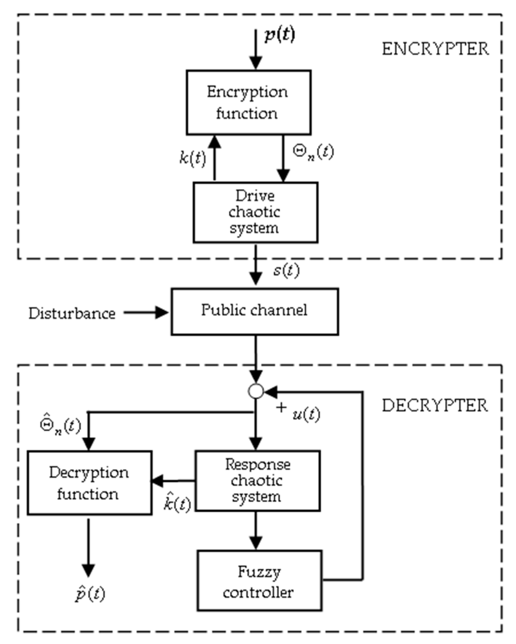
2.3. Chaotic Secure Communications

Using the property of a chaotic system, which is excessively reactive to original states, the chaos system can be applied to secure communications. This section combines cryptography technology with a chaotic system to raise the security of the dispatched message. In order to encrypt the original signal, an n-shift cipher is adopted. Figure 1 shows the block diagram of chaotic secure communications.

The encryption function is described as

$${\Theta }_n(t)=f_1(\cdots f_1(f_1(p(t),k(t)),k(t)),\cdots ,k(t))$$

(32)

where

$$f_1(p,k)=\{\begin{array}{ll}(p+k)+2\lambda & -2\lambda \le (p+k)\le -\lambda \\ (p+k)& -\lambda \le (p+k)\le \lambda \\ (p+k)-2\lambda & \lambda \le (p+k)\le 2\lambda \end{array}$$

(33)

$p(t)$ is a plaintext signal, $k(t)$ is the key signal, which is retrieved from one state of the variable of the chaotic system, n is the number of shifts, 2$\lambda$ is the range of plaintext signal plus key signal, and ${\Theta }_n(t)$ is a ciphertext signal.

By using the decryption function, the recovered signal $\widehat{p}\left(t\right)$ can be obtained. The decryption rule is described as

$$\widehat{p}(t)=f_1(\cdots f_1(f_1({\widehat{\Theta }}_n(t),-\widehat{k}(t)),-\widehat{k}(t\left)\right),\cdots ,-\widehat{k}(t))$$

(34)

where ${\widehat{\Theta }}_n(t)$ is a recovered ciphertext and $\widehat{k}(t)$ is a recovered key signal.

The chaotic secure system with extrinsic perturbation is designed as:

$$\begin{gathered} \mathit{IF}{z}_{d1}\left(t\right)\mathrm{is}{M}_{i1}\dots \dots \mathrm{and}{z}_{dp}\left(t\right)\mathrm{is}{M}_{ip} \\ \mathit{THEN}{\dot{x}}_d\left(t\right)=A_i(x_d(t\left)\right){\widehat{x}}_d(t)+B{\Theta }_n(t) \\ {y}_d\left(t\right)=C{\widehat{x}}_d(t)\hspace{1em}\hspace{1em}\hspace{1em}\hspace{1em}\hspace{1em}\hspace{1em}\hspace{1em}i=1,2,\dots ,r. \end{gathered}$$

(35)

Using fuzzy reasoning obtains the overall outputs of the polynomial fuzzy encrypter system

$$\begin{gathered} {\dot{x}}_d(t)={\displaystyle \sum _{i=1}^r{h}_i(z_d(t))}{A}_i(x_d(t\left)\right){\widehat{x}}_d(t)+B{\Theta }_n(t) \\ {y}_d\left(t\right)=C{\widehat{x}}_d\left(t\right) \end{gathered}$$

(36)

$$\begin{gathered} \mathit{IF}{z}_{r1}(t)\mathrm{is}{M}_{i1}\dots \dots \mathrm{and}{z}_{rp}(t)\mathrm{is}{M}_{ip} \\ \mathit{THEN}{\dot{x}}_r\left(t\right)=A_i(x_r(t\left)\right){\widehat{x}}_r(t)+B(u(t)+s(t))+Dn(t) \\ {y}_r\left(t\right)=C{\widehat{x}}_r(t)\hspace{1em}\hspace{1em}\hspace{1em}\hspace{1em}\hspace{1em}\hspace{1em}\hspace{1em}i=1,2,\dots ,r. \end{gathered}$$

(37)

where $s\left(t\right)$ is a transmitted message and designed as

$$s(t)={\displaystyle \sum _{i=1}^r{h}_i\left(z_d\right(t\left)\right)}{F}_i(x_d(t\left)\right){\widehat{x}}_d(t)+{\Theta }_n(t)$$

(38)

$$u(t)=-{\displaystyle \sum _{i=1}^r{h}_i\left(z_r\right(t\left)\right)}{F}_i(x_r(t\left)\right){\widehat{x}}_r(t)$$

(39)

Using fuzzy reasoning obtains the final outputs of the polynomial fuzzy decrypter system

$$\begin{gathered} \begin{array}{l}{\dot{x}}_r(t)={\displaystyle \sum _{i=1}^r{h}_i(z_r(t))}\left\{A_i\left(x_r\right(t\left)\right)-B{F}_i(x_r(t\left)\right)\right\}{\widehat{x}}_r(t)\\ +{\displaystyle \sum _{i=1}^r{h}_i\left(z_d\right(t\left)\right)}B{F}_i(x_d(t\left)\right){\widehat{x}}_d(t)+B{\Theta }_n(t)+Dn(t)\end{array} \\ {y}_r\left(t\right)=C{\widehat{x}}_r\left(t\right) \end{gathered}$$

(40)

By (36)–(40), the chaos discrepancy system with cryptography is obtained

$$\begin{gathered} \begin{array}{l}\dot{e}(t)={\displaystyle \sum _{i=1}^r{h}_i(z_r(t))}\left[A_i\left(x_r\right(t\left)\right)-B{F}_i\left(x_r\right(t\left)\right)\right]{\widehat{x}}_r(t)\\ +{\displaystyle \sum _{i=1}^r{h}_i\left(z_d\right(t\left)\right)}B{F}_i(x_d(t\left)\right){\widehat{x}}_d(t)+B{\Theta }_n(t)+Dn(t)\end{array} \\ -\left[{\displaystyle \sum _{i=1}^r{h}_i(z_d(t))}{A}_i(x_d(t\left)\right){\widehat{x}}_d(t)+B{\Theta }_n(t)\right] \\ {e}_y\left(t\right)=C\widehat{e}\left(t\right) \end{gathered}$$

(41)

In case 1, (41) can be rewritten as follows:

$$\begin{gathered} \begin{array}{l}{\displaystyle \sum _{i=1}^r{h}_i\left(z_r\right(t\left)\right)}{A}_i(x_r(t\left)\right)\widehat{e}(t)-{\displaystyle \sum _{i=1}^r{h}_i\left(z_r\right(t\left)\right)}B{F}_i(x_r(t\left)\right)\widehat{e}(t)\\ +Dn(t)\end{array} \\ +{\displaystyle \sum _{i=1}^r\left[h_i\left(z_r\right(t\left)\right)A_i\left(x_r\right(t\left)\right)-h_i\left(z_d\right(t\left)\right)A_i\left(x_d\right(t\left)\right)\right]{\widehat{x}}_d\left(t\right)} \\ +{\displaystyle \sum _{i=1}^r\left[h_i\left(z_r\right(t\left)\right)B{F}_i\left(x_r\right(t\left)\right)-h_i\left(z_d\right(t\left)\right)B{F}_i\left(x_d\right(t\left)\right)\right]{\widehat{x}}_d\left(t\right)} \end{gathered}$$

(42)

Let $z_d^T\left(t\right)=x_d\left(t\right)$ and $z_r^T\left(t\right)=x_r\left(t\right)$. The final two items will approach null when $\Vert \widehat{e}\left(t\right)\Vert \le \rho$ for the $\rho$ being very small,

$${\displaystyle \sum _{i=1}^r\left[h_i\left(z_r\right(t\left)\right)A_i\left(x_r\right(t\left)\right)-h_i\left(z_d\right(t\left)\right)A_i\left(x_d\right(t\left)\right)\right]{\widehat{x}}_d(t)\approx 0}$$

(43)

$${\displaystyle \sum _{i=1}^r\left[h_i\left(z_r\right(t\left)\right)B{F}_i\left(x_r\right(t\left)\right)-h_i\left(z_d\right(t\left)\right)B{F}_i\left(x_d\right(t\left)\right)\right]{\widehat{x}}_d\left(t\right)\approx 0}$$

(44)

Therefore, the chaotic error system with cryptography is similar to (22).

In case 2, (41) can be rewritten as (27).

3. Results

In this section, two cases of computer simulation are offered to illustrate the viability of the submitted methodology and to validate the expected $H_{\infty }$ performance. Furthermore, the sum of squares (SOS) compensator is compared with the linear matrix inequality (LMI) compensator to display the effectiveness of the submitted approach.

3.1. Case 1

In this section, the polynomial fuzzy compensator based on Theorem 1 will be executed if the synchronized discrepancies fall into a minute scope. Due to the chaos behavior of Chua’s circuit, one of the state variables will be the key signal for secure communication. The following presents the chaotic Chua’s system with perturbation.

Chua’s circuit:

$$\begin{array}{l}{\dot{x}}_1(t)={\sigma }_1(-x_1(t)+x_2(t)-f(x_1(t)))\hfill \\ {\dot{x}}_2(t)=x_1(t)-x_2(t)+x_3(t)\hfill \\ {\dot{x}}_3(t)=-{\sigma }_2{x}_2(t)\hfill \end{array}$$

(45)

With a nonlinear resistor $f(x_1(t))=g_b{x}_1(t)+0.5(g_a-g_b)$$\cdot (\left|x_1(t)+1\right|-\left|x_1(t)-1\right|),$ where ${\sigma }_1=10$, ${\sigma }_2=14.87$, $g_a=-1.27$, and $g_b=-0.68$. The nonlinear term $f(x_1(t))$ of Chua’s circuit satisfies ${\lim }_{\underset{x\in \mathsf{\Omega }}{x_1(t)\to 0}}(f(x_1(t))/x_1(t))=g_a$. Then, $f(x_1(t))$ is taken as $\phi (x_1(t))$ with

$$\phi (x_1(t))\equiv \{\begin{array}{c}f(x_1(t))/x_1(t),\\ g_a,\end{array}\begin{array}{c}{x}_1(t)\ne 0\\ x_1(t)=0\end{array}$$

(46)

Select $x_1(t)$ as the premise state and design the fuzzy set to be $M_1(x_1(t))$=$(1/2)(1-(\phi (x_1(t))/d))$ and $M_2(x_1(t))$ $=1-M_1(x_1(t))$ with $d={\sup }_{x_r\in \mathsf{\Omega }}\left|\phi \left(x_1\right)\right|=3$.

Deliberate synchronization of two fuzzy Chua’s systems in which the drive and response systems are represented by (16) and (18), respectively. Let the system matrices be designed as:

$$A_1(x_r(t\left)\right)=A_1(x_d(t\left)\right)=\left[\begin{array}{ccc}(d-1){\sigma }_1& {\sigma }_1& 0\\ 1& -1& 1\\ 0& -{\sigma }_2& 0\end{array}\right],$$

(47)

$$A_2(x_r(t\left)\right)=A_2(x_d(t\left)\right)=\left[\begin{array}{ccc}-(d+1){\sigma }_1& {\sigma }_1& 0\\ 1& -1& 1\\ 0& -{\sigma }_2& 0\end{array}\right],$$

(48)

$$B=\left[\begin{array}{c}1\\ 0\\ 0\end{array}\right],C=\left[\begin{array}{ccc}1& 1& 0\end{array}\right].$$

(49)

The original conditions of the response system are arbitrarily selected as $x_r(0)={[\begin{array}{ccc}-0.1& -0.1& -0.1\end{array}]}^{\mathrm{T}}$ and those of the drive system are arbitrarily selected as $x_d(0)={[\begin{array}{ccc}0.1& 0.1& 0.1\end{array}]}^{\mathrm{T}}$. If there exists an extrinsic perturbation, which is a pulse with amplitude 40 occurring from the 35th sec to the 36th sec, we assume the perturbation appeared in the first state, which means that $D={\left[\begin{array}{ccc}1& 0& 0\end{array}\right]}^T$. The $H_{\infty }$ achievement is chosen as $\xi =0.2$ for better perturbation attenuation. The plaintext signal is set as p(t) = 2sin(t) for better demonstration. The number of shifts is selected as n = 30 for better security. The key signal is retrieved from the first state of the Chua’s circuit, i.e., k(t) = $x_{d1}(t)$ and $\widehat{k}\left(t\right)$ = $x_{r1}\left(t\right)$. The range of plaintext signal plus the key signal is estimated as $\lambda$ = 8. Then, utilizing Theorem 1 we acquire the compensator ($F_1,F_2$) and the matrix $R$ whose eigenvalues are positive. To compare with the SOS methodology, the LMI-based compensator is procured from the literature [8].

SOS-based compensator ($\xi$ = 0.2)

$$F_1=\left[\begin{array}{ccc}61.6093& 27.5899& 0.0058\end{array}\right]$$

(50)

$$F_2=\left[\begin{array}{ccc}8.5459& 29.5633& -0.0734\end{array}\right]$$

(51)

$$\mathit{R}=\left[\begin{array}{ccc}2.7517& 1.0915& -0.0247\\ 1.0915& 1.4974& -0.0285\\ -0.0247& -0.0285& 0.0725\end{array}\right]$$

(52)

LMI-based compensator ($\xi$ = 0.2)

$$F_1=\left[\begin{array}{ccc}38.2871& 28.5285& 0.8880\end{array}\right]$$

(53)

$$F_2=\left[\begin{array}{ccc}-21.7129& 28.5285& 0.8880\end{array}\right]$$

(54)

$$\mathit{R}=\left[\begin{array}{ccc}0.2500& 0.2272& -0.0000\\ 0.2272& 0.2758& -0.0009\\ -0.0000& -0.0009& 0.0047\end{array}\right]$$

(55)

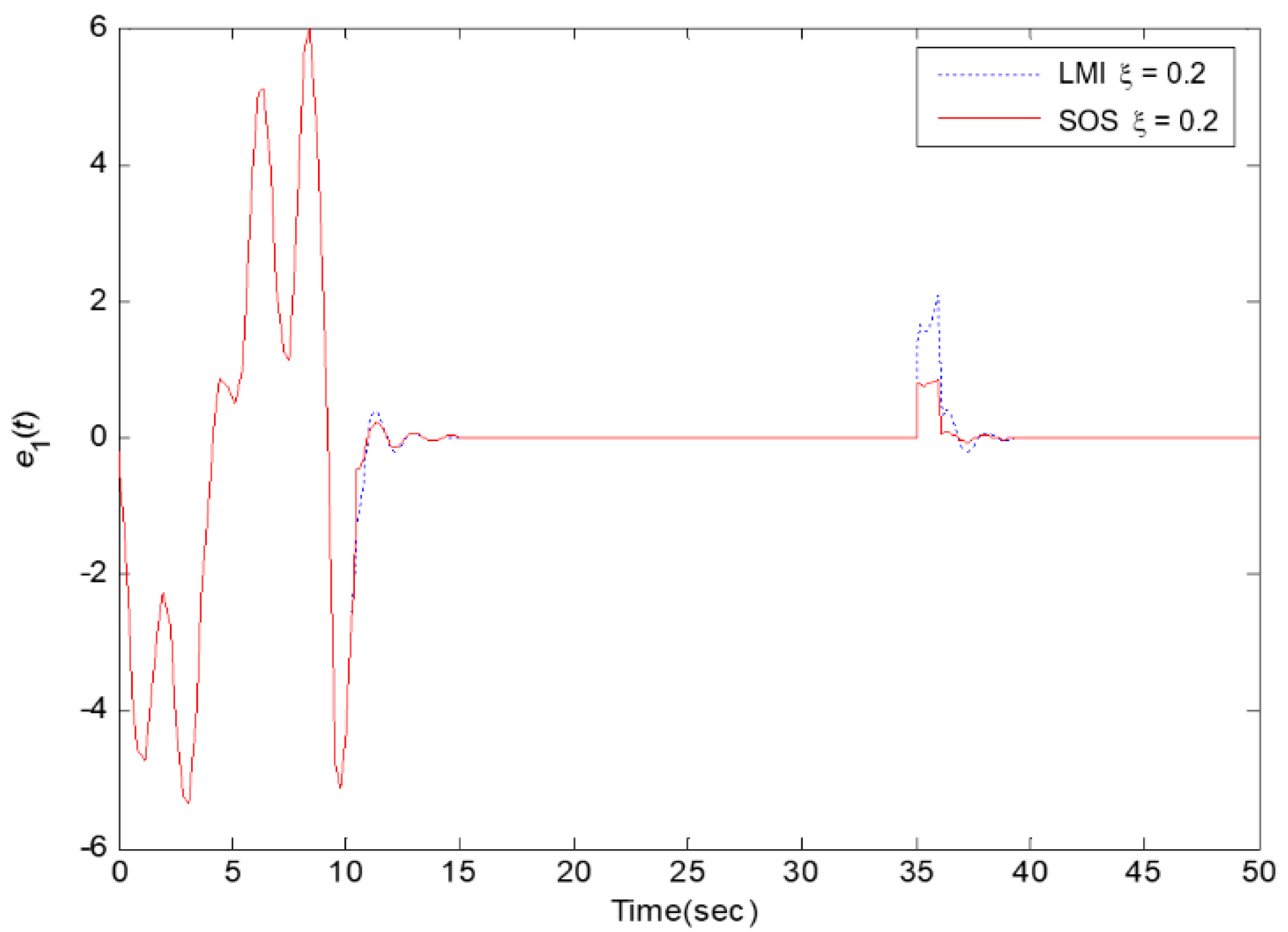
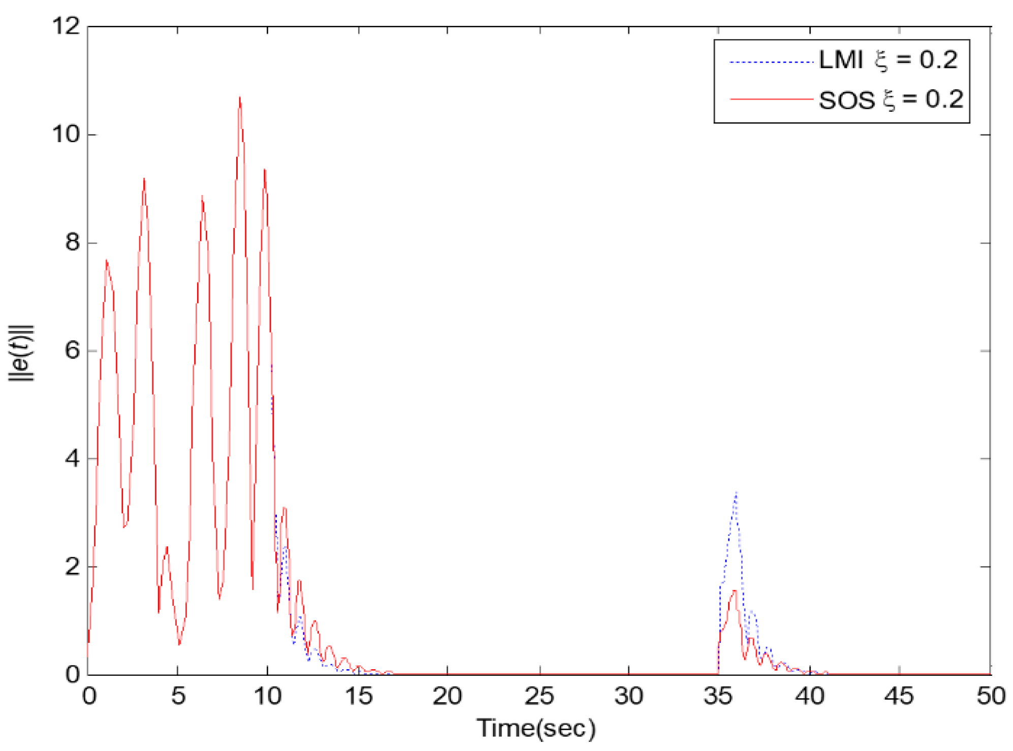
Figure 2, Figure 3 and Figure 4 display the compared responses of the perturbation decay achievement. Figure 5 shows that the operation commences at t = 10 s, but the control signal is joined around 10.5 s when $\Vert \widehat{e}\left(t\right)\Vert \le 4$. To evaluate the $H_{\infty }$ performance of proposed method, an integral square error (ISE) is defined as follows:

$$\mathrm{ISE}={\displaystyle {\int }_{35}^{40}\Vert e\left(t\right)\Vert }\mathrm{d}t$$

(56)

The value of ISE via the SOS method is 3.02 and the value of ISE via the LMI method is 6.17. Apparently, the submitted SOS-based compensator has better perturbation rejection.

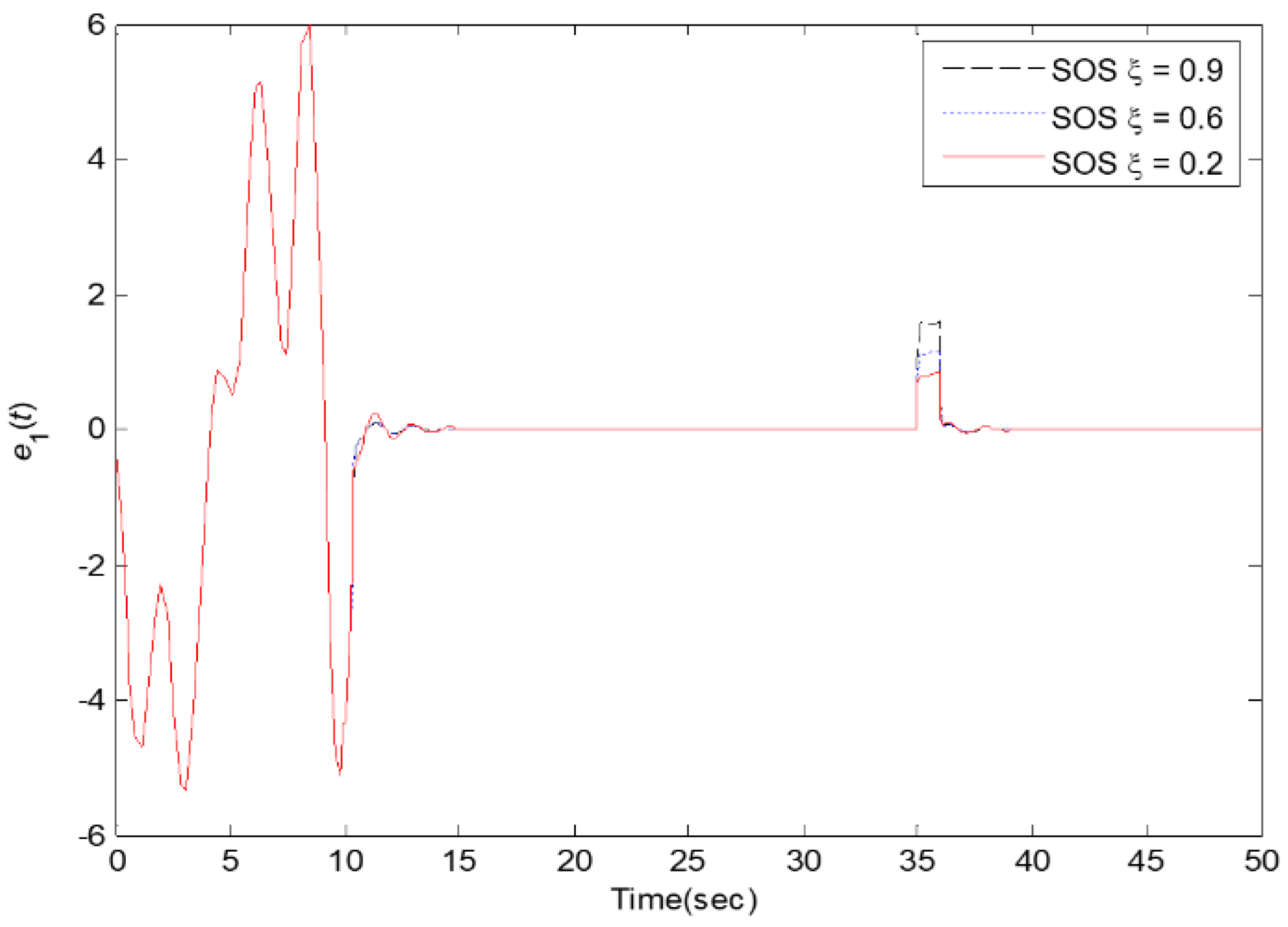
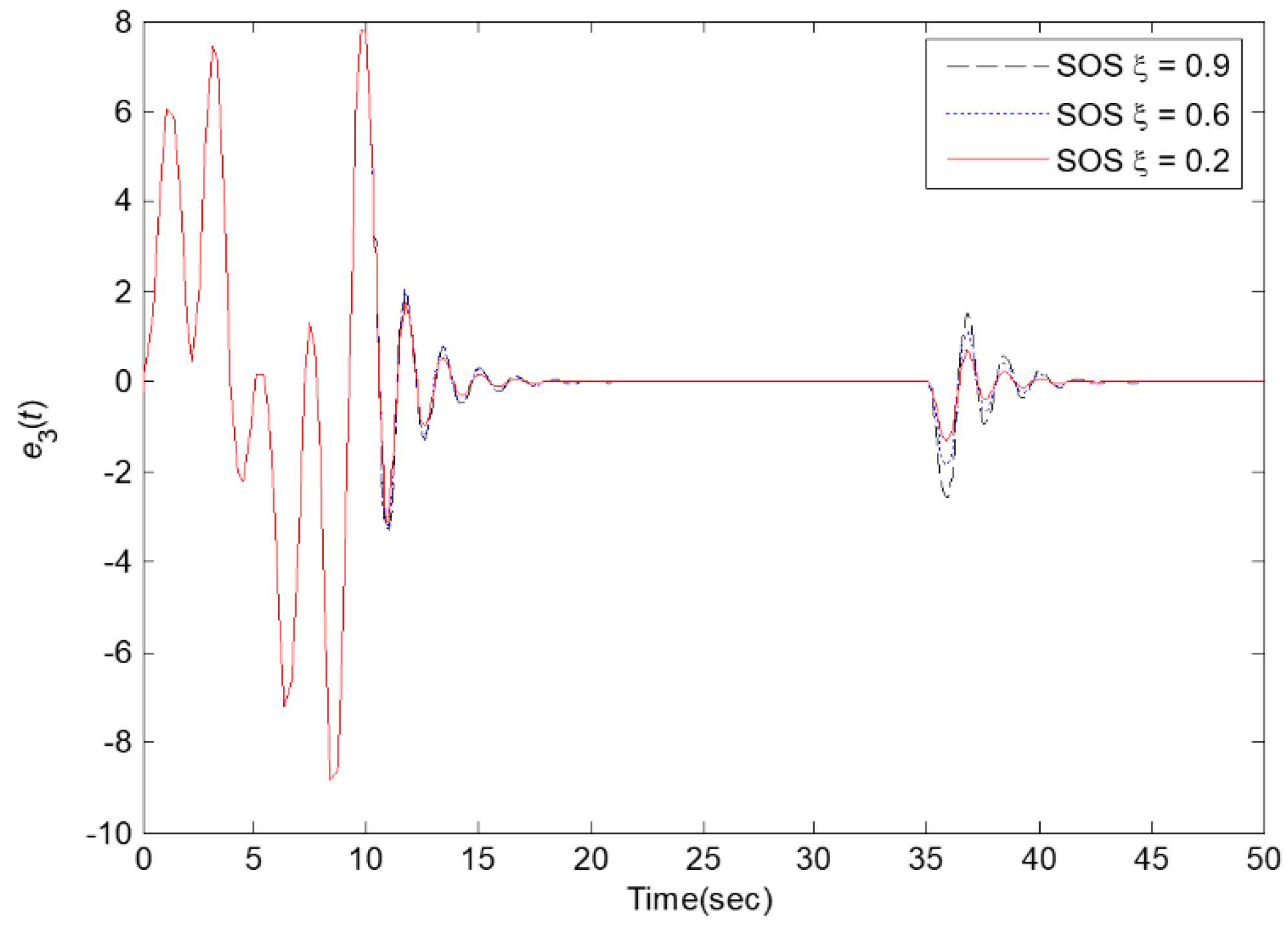
Based on Theorem 1, the compensator ($F_1,F_2$) and the matrix $R$, whose eigenvalues are positive at various $\xi$, are obtained as follows. Figure 6, Figure 7 and Figure 8 show the $H_{\infty }$ achievement at various $\xi$ cases with the compensators operating at $t\ge 10$. Obviously, the perturbation attenuation achievement will be increased when the value of $\xi$ is decreased.

SOS-based compensator ($\xi$ = 0.6)

$${\mathit{F}}_1=\left[\begin{array}{ccc}48.2971& 15.2806& -0.0009\end{array}\right]$$

(57)

$${\mathit{F}}_2=\left[\begin{array}{ccc}-6.8468& 15.6567& -0.0164\end{array}\right]$$

(58)

$$\mathit{R}=\left[\begin{array}{ccc}12.5995& 2.1331& -0.0633\\ 2.1331& 4.3748& -0.0695\\ -0.0633& -0.0695& 0.2725\end{array}\right]$$

(59)

SOS-based compensator ($\xi$ = 0.9)

$${\mathit{F}}_1=\left[\begin{array}{ccc}41.4964& 13.4478& 0.0136\end{array}\right]$$

(60)

$${\mathit{F}}_2=\left[\begin{array}{ccc}-13.3518& 13.7721& 0.0033\end{array}\right]$$

(61)

$$\mathit{R}=\left[\begin{array}{ccc}16.6246& 2.3470& -0.0736\\ 2.3470& 5.3791& -0.0830\\ -0.0736& -0.0830& 0.3425\end{array}\right]$$

(62)

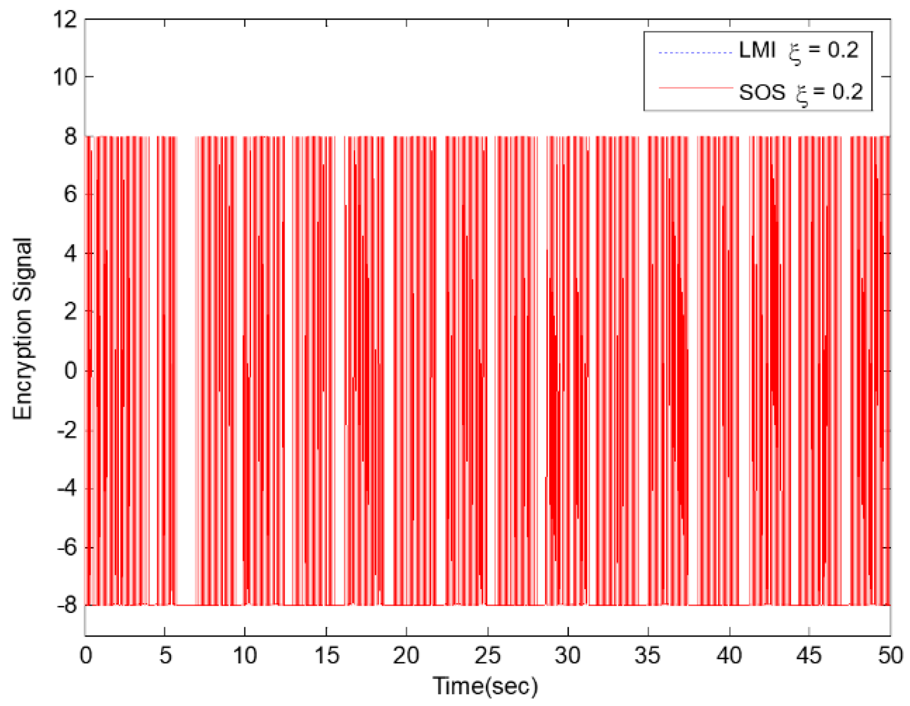
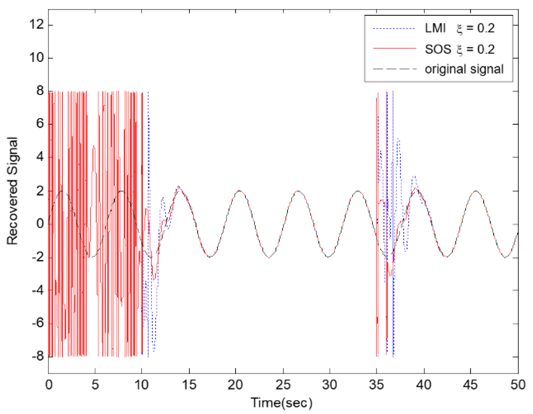
Figure 9 shows the encrypted signal. Figure 10 shows the recovered signal with perturbation rejection. Figure 11 and Figure 12 show that the SOS method is more relaxed than the LMI method. The stability criteria via SOS are more universal than those via LMI. That is, the result from the LMI method is also a solution for the SOS-based method. From the above outcomes, we confirm that the proposed SOS-based fuzzy compensator also offers larger feasible space and achieves better perturbation attenuation performance for Chua’s system.

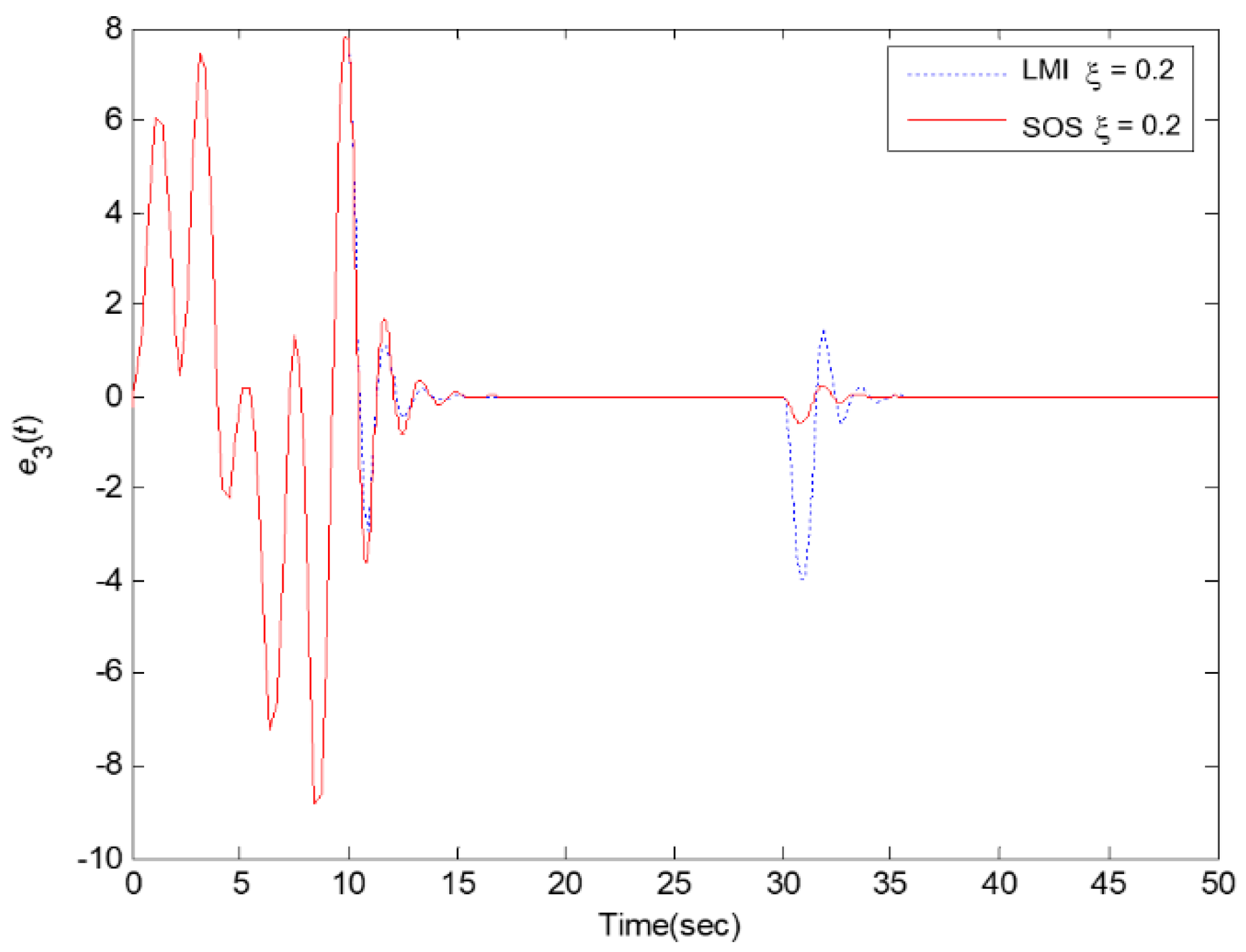
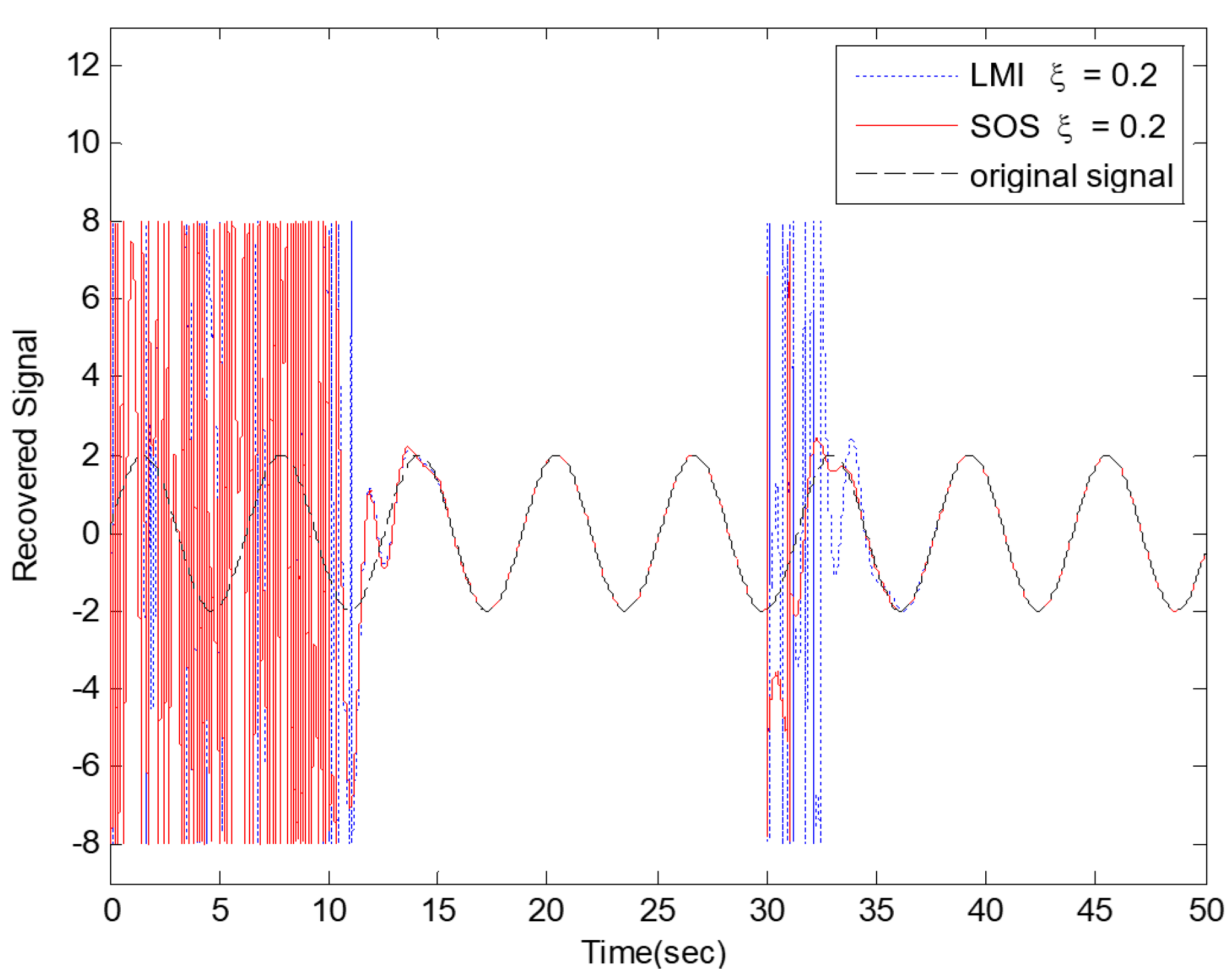
3.2. Case 2

In this section, the polynomial fuzzy decrypter based on Theorem 2 will be executed if the synchronized discrepancies exceed the minute scope of case 1. The fuzzy model of two Chua’s circuits and the simulation parameters (such as the initial states, r, p(t), n, $\lambda$, k(t), and $\widehat{k}(t)$) are the same as case 1 except that the extrinsic perturbation is a pulse with amplitude 40 and occurs from the 30th sec to the 31th sec.

Thus, applying Theorem 2 could acquire the compensators ($F_1,F_2$) and the matrix $R$ whose eigenvalues are positive. To contrast with the SOS methodology, the LMI-based compensator is procured from the literature [8].

SOS-based compensator ($\xi$ = 0.2)

$$F_1=\left[\begin{array}{ccc}103.2541& 96.2763& -0.1880\end{array}\right]$$

(63)

$$F_2=\left[\begin{array}{ccc}96.5163& 91.0441& -0.1315\end{array}\right]$$

(64)

$$\mathit{R}=\left[\begin{array}{ccc}0.9843& 0.0512& -0.0004\\ 0.0512& 1.0614& -0.0145\\ -0.0004& -0.0145& 0.0713\end{array}\right]$$

(65)

LMI-based compensator ($\xi$ = 0.2)

$$F_1=\left[\begin{array}{ccc}34.7109& 25.1400& 0.8711\end{array}\right]$$

(66)

$$F_2=\left[\begin{array}{ccc}-25.2891& 25.1400& 0.8711\end{array}\right]$$

(67)

$$\mathit{R}=\left[\begin{array}{ccc}0.2926& 0.2618& -0.0000\\ 0.2618& 0.3388& -0.0013\\ -0.0000& -0.0013& 0.0070\end{array}\right]$$

(68)

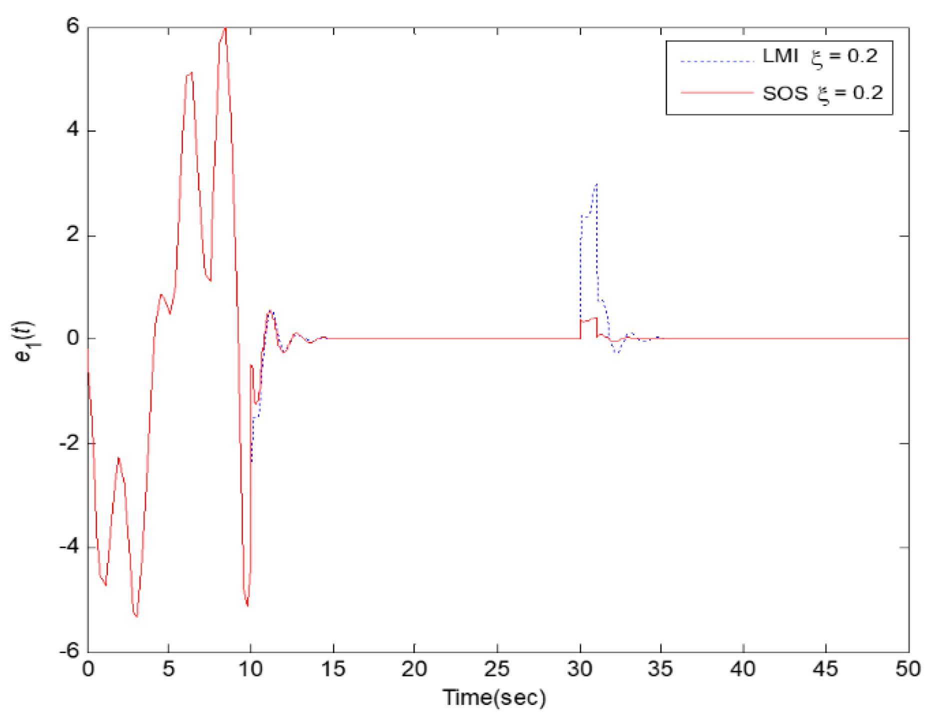
Figure 13, Figure 14 and Figure 15 show the comparison results of the perturbation attenuation performance for Chua’s circuit. Figure 16 shows the recovered signal with perturbation rejection for Chua’s circuit. Moreover, the SOS approach is superior to the LMI approach for Chua’s circuit.

4. Conclusions

This study displayed the $H_{\infty }$ synthesis of a polynomial fuzzy compensator through the sum of squares (SOS) approach for synchronization of chaos systems and secure communications. The SOS-based criteria with $H_{\infty }$ performance was proposed against the extrinsic perturbation through the polynomial Lyapunov function. Based on the norm of synchronization discrepancies, the chaos synchronization was divided into two cases. Numerical simulation showed that the synchronization discrepancy can converge to zero, and the signal can be recovered under extrinsic perturbation in either case 1 or case 2. The feasible space of the proposed stability conditions via SOS was larger than that of the existing stability conditions via linear matrix inequality (LMI). Moreover, the $H_{\infty }$ performance of the proposed SOS chaos control system was superior to that of the existing LMI chaos control system.