
Infection Units: A Novel Approach for Modeling COVID-19 Spread


1
Department of Chemical Engineering, Ben-Gurion University of the Negev, Beer-Sheva 84105, Israel
2
Research Centre CIAIMBITAL, Department of Chemical Engineering, University of Almería, 04120 Almería, Spain
*
Author to whom correspondence should be addressed.
Processes 2021, 9(12), 2272; https://0-doi-org.brum.beds.ac.uk/10.3390/pr9122272
Submission received: 26 November 2021
/
Revised: 11 December 2021
/
Accepted: 12 December 2021
/
Published: 17 December 2021
(This article belongs to the Special Issue Mathematical Modeling and Numerical Research of Heat Transfer in Heterogeneous Flows)
Abstract
:A novel mechanistic model of COVID-19 spread is presented. The pool of infected individuals is not homogeneously mixed but is viewed as a passage into which individuals enter upon the contagion, through which they pass (in the manner of “plug flow”) and exit at their recovery points within a fixed time. Our novel concept of infection unit is defined. The model separately considers various population pools: two of symptomatic and asymptomatic infected patients; three different pools of recovered individuals; of assisted hospitalized patients; of the quarantined; and of those who die from COVID-19. Transmission of this disease is described by an infection rate function, modulated by an encounter frequency function. This definition makes redundant the addition of a separate pool for the exposed, as done in several other models. Simulations are presented. The effects of social restrictions and of quarantine policies on pandemic spread are demonstrated. The model differs conceptually from others of the kind in the description of the transmission dynamics of the disease. A set of experimental data is used to calibrate our model, which predicts the dynamic behavior of each of the defined pools during pandemic spread.
1. Introduction
It seems that COVID-19 is one of the hardest health problems that humanity has had to deal with throughout its history, not due to the severity of the disease, nor its rate of spreading, but because of its global impact, as it has been the most rapidly widespread pandemic. This is the case due to the 21stcentury combination of accessible, advanced transportation technology and the large volume of international travel for both business and pleasure—a blatant feature of modern consumer societies. Currently, almost all the countries in the world are engaged in trial-and-error processes, in which sanitary measures (including vaccination rate) are competing with economic activities of all kinds in battles between public health management and sustainable population maintenance [1]. There is a need for a macro-model that describes, as closely as possible, the whole of this complex issue [2,3]. Within such a macro-model, the modelling of the epidemiologic aspect and its particularities is of extreme relevance. The textbook of Keeling and Rohani [4] is an excellent presentation of the state of the art at the time of its publication and remains a very valuable source. However, the surge of the COVID-19 pandemic led to an extraordinary number of scientific publications dealing specifically with the matter.
The number of research papers published on COVID-19 is vast, and their scope is broad [5]. Sometimes the spread of a pandemic has tendencies that seem random. Therefore, statistical methods have been applied to predict the spread of such diseases as they take multiple factors into account by means of time-series models, multivariate linear regressions, gray forecasting models, backpropagation neural networks and others. However, the aforementioned statistical tools seem to be insufficient for analyzing pandemic randomness and these models are difficult to generalize, as noted by Ceylan [1]. She claims that the COVID-19 prevalence in several European countries may be described using variants of an autoregressive integrated moving average (“ARIMA”) model, a time-series-type model [1]. Wu et al. simulated the expansion of COVID-19 across the most populated Chinese cities connected by airlines, using what they called “a metapopulation model” with SEIR variables. SEIR stands for susceptible (individuals that are vulnerable to viral infection), exposed (individuals that have been invaded by the virus, but do not shed virions and therefore are not infectious yet), infected (individuals that can transmit the virus) and recuperated (individuals that have been through the disease and are not infectious anymore) [6]. A metapopulation model is one that considers regional subgroups that are interacting. The basic calculations applied Markov chain Monte Carlo methods. Models of this type are called “agent-based” models because they focus on the movement of/and contact between individuals. They require laborious calculations that provide a geographical aspect to pandemic spread.
Hunter et al. made a detailed comparison of equation-based models (EBM) versus agent-based models (ABM) [7]. They are two modelling methods widely reported to model the spread of infectious diseases. An ABM consists of emulating the individual behavior of a set of agents that make up the system under consideration. By contrast, EBM is a set of equations whose execution consists of evaluating them. Moreover, recently Tsori and Granek [8] among others commented that most of the deterministic models are of the SEIR-type; they also stressed the fact that a “perfect mixing”, that is “total homogeneity” in each of the pools, is always assumed [8]. They pursue mitigation of this limitation by formulating “a continuous spatial model based on nearest-neighbor infection kinetics,” which leads to a reaction-diffusion-type description of pandemic spread. This enables the description of the spatial spread of a pandemic; their results show the two-dimensional spread across an actual geographical map. Nevertheless, their model maintains the same mathematical format as the SEIR-type models by describing the infected (I) pool as a mixed compartment, in the sense that an individual classified as “infected” may leave this compartment independently of his/her “external age”, i.e., the time spent in it [9]; here, “age” is defined as the average time an infected individual spends in the I pool (The significance of this point is explained below).
The Manenti et al. model describes the entire population of the world as a perfectly mixed batch reactor [10] and reaches formulations that are equivalent to the classic SEIR or SIR models, as may be expected. Cao et al. proposed an improvement with their 6-compartment SEIR-type model, by adding a pool of quarantined patients [11]. They used a time-series analysis exponential smoothing method and the ARIMAX model (often used in statistical modeling) to analyze changes that occur over time.
A considerable improvement in SEIR-type models was achieved by Ivorra et al. [12]. They called it the θ-SEIHRD model and it was based on their previously published Bi-CoDis model [13]. In the θ-SEIHRD model, they added seroprevalence as a measured variable, which is a very important addition to a system with a scant number of measured variables. Most recently, Sen and Sen (2021) published a modification of the SEIRD model, in which a quarantine (Q) pool is included [14]. They claim the data fits satisfactorily with the recorded changes in the infected, recovered and dead in five countries, but comes at the cost of significant variation in some of the rate constants for different countries [14]. This variation, sometimes of several orders of magnitude, is explained by the authors as related to marked lifestyle differences. These outcomes stress the difficulties in the formulation of a general model that describes all the manifestations of such pandemics. Note when reading their paper that their definition of “quarantine” differs from the usual one found in the literature. For Sen and Sen, it represents the isolation enforced after infection is confirmed, rather than preventive isolation, due to suspicion of potential contagion [14].
In the present work, we focus on the basic mechanisms of pandemic spread and present a deterministic model with a novel approach. Our model differs conceptually in the manner of description of the transmission dynamics of the disease, the key being the “external age distribution” of the individuals exiting the I pool [9]. This requires a formulation that is different from that of the various SEIRD models mentioned above [12,14], among others, which assume that all the population pools are perfectly mixed.
The Flow Dynamics of the Infected (I) Population Pool
Here, we try to focus on one basic concept implied in the SEIR formulation and propose an alternative. The SEIR-inspired models, in all their variants, collide with the basic observation that the duration of this illness is an almost constant number of days [15,16]. The well-known SEIR models describe distinct pools of the susceptible (S), exposed (E), infectious (I) and recovered (R) and sometimes additional pools--all of them defined as completely mixed. In a completely mixed continuous system, the systemic response to a pulse disturbance will always have a bell shape (in the case of an ideal instantaneous pulse, to a descending exponential), as described in basic textbooks [4,17]. This bell shape represents the “age distribution” within the compartment; consequently, the “age” of the individuals leaving the I pool will show a wide distribution. There would be individuals who stay in that pool a very short time, near zero and others who stay in the pool a very long time, near infinite. This blatantly contradicts our knowledge about the behavior of COVID-19 and other Coronaviruses that produce sicknesses with quite defined durations [15].
The I pool, as it will be defined here, has an inlet of individuals from the pool of the susceptible, S, and outlets to other pools, but has a completely different behavior. In the terminology of process engineering, the exhibited behavior is called “a plug flow system” (resembling a conveyor belt), such as a moving walkway transporting infected individuals. The main characteristic defining such a system is its population dynamics, i.e., the homogeneity of the “age” of the individuals leaving the compartment. The “age” of the elements leaving the system cluster around a certain mean “residence time”, tr, with relatively small variance. In practice, it is well known that a COVID-19-infected individual stays as such for a finite and quite defined period of time, as estimated in the literature on the basis of experimental findings [15]. Though there may be some individual variations in the case of COVID-19, this period of time seems to be consistently around two weeks [18]. The state of the patient changes throughout this period and may lead either to recovery or to a more severe state and then, either to a full recovery or to death. The actual events during a normal I period take place along one clear timeline in an orderly manner. This is a basic characteristic of the illness, and the SEIR models fail to describe it. Such models may fit the dynamics of infection in the case of a population pool over long periods of time but cannot describe the short-term dynamics. Here, we present an alternative approach that overcomes this weakness.
2. An Alternative Approach
2.1. The I Pool
A “plug flow model” is a diametrically opposed alternative to the totally mixed compartments that characterize the SEIR-type models. In a plug flow system, all the elements that enter a compartment will leave it after residing in it a unique finite time, tr, the same for all. In terms of our model, all the infected individuals will remain in this condition approximately tr days.
In an ideal plug flow situation, any change in the input at t = 0 will produce the same (or similar) signal at the outlet, at t = tr. In other words, the “age” of each infected individual will increase steadily from 0 to tr, which represents the period during which he/she was a member of the I pool. In practice, there will obviously be a certain distribution around the mean value but, in this version of the model, we disregard it.
For convenience in formulating this model, a dimensionless residence time τ (τ = t/tr) was defined, only and specifically for the description of the infection in an individual staying in the I pool. The value of τ varies between 0 (at the inlet of the pool I, i.e., at the start of the infection) and 1 (at the outlet of the pool I). Therefore, τ = 1 is equivalent to tr. τ runs parallel to time t, starting from zero every time a susceptible individual becomes infected. The time span (0 < t < tr) must be treated somewhat differently, as shown below.
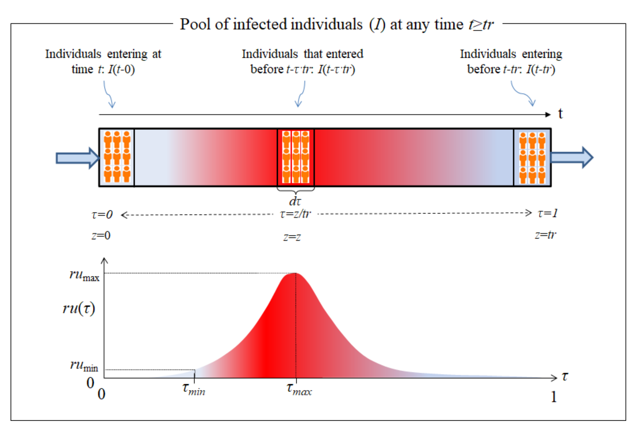
Based on the definition of τ, schematic Figure 1 shows how individuals, with different I ages, are located throughout the entire I pool (top of the figure) at a given time t. At the bottom of Figure 1, a single individual is shown in transit through the course of the illness (0 < τ < 1). For any t > tr, a record of all the data in the entire I pool would show the whole length of the passage or moving walkway that represents the pool of the infected, occupied by infected individuals of increasing “age” (“residence time” in the I pool). In other words, at the pool inlet (τ = 0), I(t) newly infected would be entering, while the infected individuals located within 0 < τ < 1 would be those who entered the pool at an earlier time (t − τ·tr). The “oldest” individuals, after tr days of illness, are found at the exit, τ = 1, leaving the I pool. For the special case in which the time elapsed from the start of the pandemic is exactly t = tr, those individuals who are just about to leave the I pool (at τ = 1) will be those same susceptible individuals who had just become infected and started their infection period at t = τ = 0.
There is another particular case that occurs when the time elapsed from the beginning of the pandemic is t < tr. In this case, “patient zero” is located on the “moving walkway” at τ = t/tr and has not yet left the I pool, the end of which is located at τ = 1. As result, the “moving walkway” is empty in the interval [τ, 1]. Other than this special case, all patients start the transit through the I pool at τ = 0 and exit at τ = 1.
Before describing the I pool, we must introduce the “infection unit” (U), defined as the amount of COVID-19 virus released by an infectious individual in any way or form, having the capacity to cause the conversion of susceptible (S) individuals into infected (I) ones. This definition is inspired by the “Photosynthetic Unit” (PSU) concept, sometimes called photosynthetic factories, that is widely accepted in photosynthesis modelling. A PSU is defined as the sum of light-trapping systems, reaction centers and associated apparatus that are activated by a given amount of light energy to produce a certain quantity of photoproducts. This PSU concept seems intangible, yet it has produced excellent practical results in the modeling of photobioreactors [19,20,21]. We consider that the same may be true for our viral “infection unit” concept, U. An infected individual moves through the I pool, releasing U at a certain rate, ru(τ). This rate is only the result of the disease incubating in his body during his/her transit through the illness (from τ = 0 to τ = 1) and will, therefore, not be affected by any of the variables in the model. A shifted Gaussian function, as shown in the lower part of Figure 1, was chosen arbitrarily to represent ru(τ). Other functions may be used without changing the underlying concept.
The curve plotted in Figure 1 concurs with the actual behavior of the virus. Once the invading virus enters the body, it requires a certain amount of time to locate and penetrate its target cell, before activating its cellular machinery to produce the first generation of native virus. The durations of some of those steps have been reported for other viruses [22]. Then, additional time (an “eclipse phase”) necessarily follows, during which more cells must be infected and finally reach τmin, the point in time at which the actual dissemination of the virus from the ill person’s body takes place. At this stage, the infection may be detected in the case of symptomatic patients, or by RT-PCR test (reverse transcription polymerase chain reaction) in asymptomatic ones. Since ru(τ) starts at zero and at the end of the infectious period it will once again be zero or close to it, it is obvious that, at some point (τ = τmax), there will be a peak in viral dissemination rate (rumax), followed by a ru(τ) decrease. Here, it is assumed that there is a certain minimum rate of U production, below which there is no infectivity (rumin), as shown in Figure 1. At the end of the period (τ = 1), the patient recuperates and passes into the R pool, unless his/her health deteriorates, a situation will also be considered below. The definition of ru(τ) makes redundant the addition of a separate pool for the “Exposed”, as was done in several other models.
The generation of U is necessary, but on its own, it is not enough to transmit an infection. For transmission to occur, the presence of a susceptible individual is also required. In the SEIR models, the presence of susceptible individuals is permanent, as implied by the assumed kinetic form of the infection rate, where the product I times S appears. As long as S is not null, some degree of infection occurs. Nonetheless, in practical, interpersonal encounters, an infected individual will not always be within physical infectivity range, nor will the quantity of the U released by an infectious person be enough to effectively transmit this viral disease. This fact is expressed by means of our encounter frequency function, f(t), where t is the timeline along which the pandemic progresses. We will focus on the case of a typical, asymptomatic person infected with COVID-19.
The transmission of this infection via individuals who carry the virus, but are asymptomatic, is a characteristic of COVID-19 and was seldom seen in the SARS and MERS outbreaks. As long as the disease has not yet been diagnosed, no special insolation measures are taken. It may be assumed that there are different types of encounters between infected and susceptible members in a community related to lifestyles, usual daily routines, essentially repetitious in nature (e.g., work, study, shopping, hobbies, regular schedules and means of transportation). The importance of such regular routines has been recognized Backer et al. [23]. There are also certain non-routine activities, often involving a larger number of people (e.g., weddings, parties, dinners, etc.). The abovementioned “super-spreading events” can easily be included here in addition to individual singularities but here, for the sake of simplicity, we intentionally present only the repetitive daily encounters as periodic functions. One of the simplest formulations for this encounter frequency function, f(t), is:
In expression (2), the influence of the restrictions imposed on social contacts (“social distancing”) and their impact on the behavior of the population may be accounted for in a(t), which is instrumental in the modulation of the infection rate constant (KSI). The need for this modulation has already been indicated in the literature [24,25]. We adopted the following function based on another recent report [26]:
where it is assumed that, once a restriction has been imposed by the authorities and it starts on a certain fixed day (tc), the level of social contact will decay at a rate of λ from a starting value βo, tending towards a limit value of βf. Obviously, the greater the severity of the restrictions, the higher the λ value and the lower the βf value. The Equation (3) above may be used for i consecutive constraints; with λi values for each interval tci − tci+1, on which the i restriction is set. As previously detailed [25], to improve the flexibility of Equation (3), the integration interval may be split into sub-intervals with widths that do not have to coincide exactly with the days on which the restrictions were decreed.
It should also be taken into account that not every infected person in the I pool will transmit the disease. In this paper, we assume that all diagnosed patients (Id), are under proper care, completely isolated, in which case f(t) = 0 and they cease to be contagion factors; the same applies to all assisted, hospitalized patients. However, infected individuals who have not yet been identified as such because they are not showing blatant symptoms, are considered in the present version of this model as being the only factors of pandemic transmission.
The U defined above are generated at the rate of ru(τ), produced during the evolution of the disease within the body of each patient during his/her passage through the illness (from τ = 0 to τ = 1); as such, this rate is not affected by any of the variables in the model. By definition, ru represents the rate of generation of the U by a single infected individual. In order to calculate the total U generation, the number of infected individuals is required. The number of asymptomatic infected individuals at time t, who are at stage of the illness is Ind(t − τ·tr). It is convenient to define the total number of U generated by individuals in the state of infection at a given time t as U(t,):
Here, Ind(t − τ·tr) is the number of Ind who entered the Ind pool at an earlier time (t − τ·tr) and, as a result, they have an “infectivity rate” of ru(τ) at a given time t, where is the dimensionless “residence time” (t/tr) in the Ind pool, that runs along time, taking values from = 0 to = 1, as previously explained. Note that Equation (4) renders the U production rate of infected individuals at time t in state . Multiplying by the encounter function, we get the number of U able to transmit infection. Integrating over the range of we obtain the total rate of infection at any time, t > tr, within the Ind pool:
Equation (5) shows that, for the calculation at a time t, we must refer back to past values of Ind(t) (before t), following Equation (4). (The precise numerical calculation procedure is detailed later on in this paper.) Note that, for t < tr the number of infected individuals coincides with the initial condition Ind(0). For the interval 0 < t ≤ tr, we have modified Equation (5) as follows:
The shape of Equation (5) allows to include this model in the category of Models with History [4].
2.2. Description of the Model
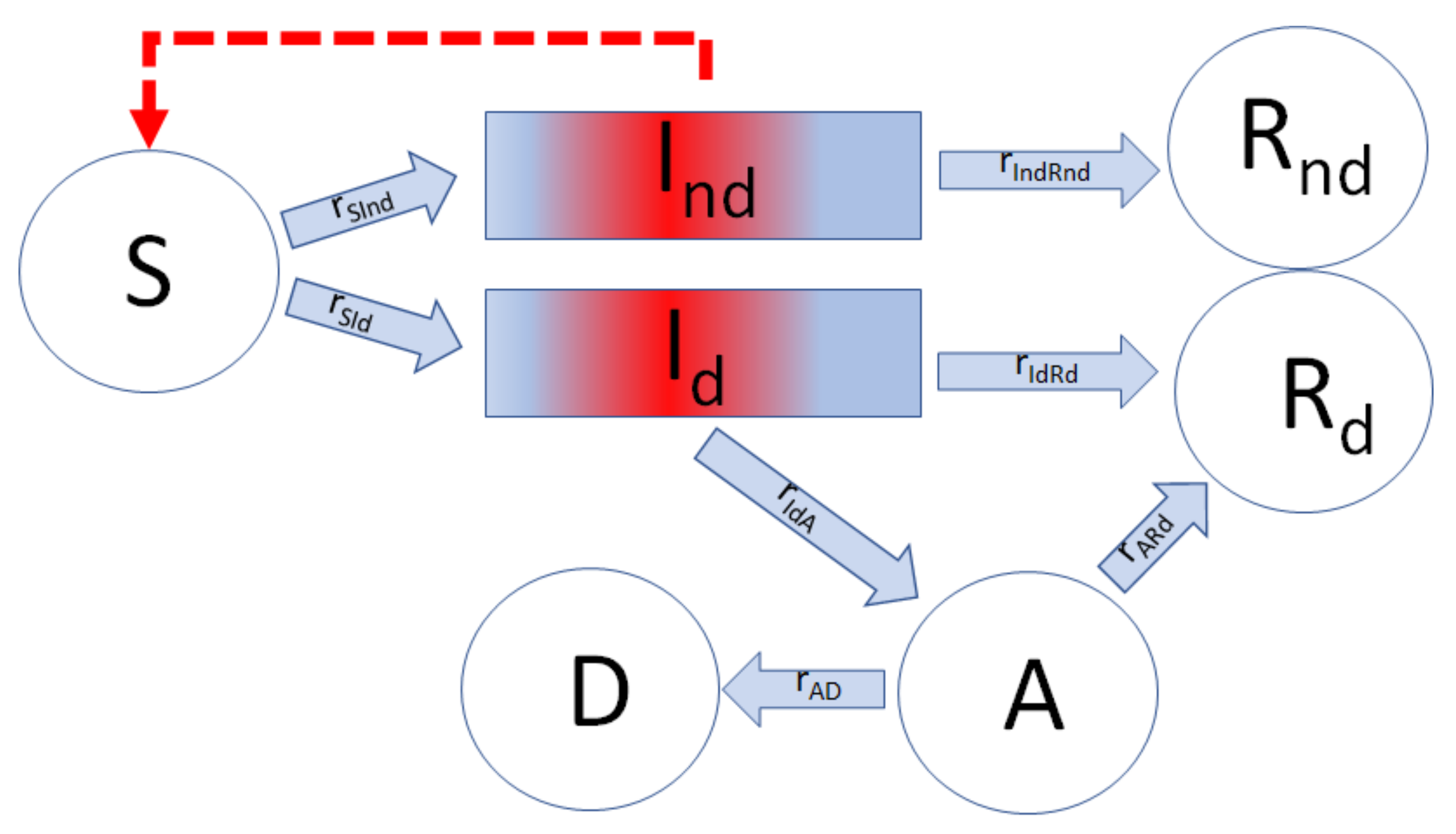
The history of a single member of the entire I pool, from the time of his/her infection (τ = 0), is presented here. At this stage, it is important to note the distinction between asymptomatic individuals, who are unaware of their medical conditions and to whom no social-distancing restrictions are yet applied, and those detected patients, identified as having COVID-19, who are assumed to be isolated. The general scheme of the model may be seen in Figure 2 below.
In Figure 2, the rectangles indicate that the individuals in both I pools behave as described in Figure 1 in regard to time dependence, tr, while the circles symbolize other pools, in which the exit time, t, is not dependent on the “residence age”; that is, the sub-population is “perfectly mixed”.
That fraction of infected individuals who are not diagnosed, either because they were asymptomatic or because the symptoms were mild and went unnoticed, constitute the pool, Ind. They are, however, contagious and can infect the susceptible population (S) in accordance with the U dissemination mechanism described above. All the undiagnosed individuals in the Ind pool recover after a time of tr, when they become members of the corresponding pool of the detected recovered patients, Rnd. The remainder of the total infected, Id, develop characteristic symptoms after the period of incubation and are then isolated; thus, we assume that they no longer serve as factors in contagion. After tr, when the Id recuperate, they enter the pool Rd. An alternative case is when a patient suffers a complication during his/her illness (related or not to pre-existing problems) and the patient’s health deteriorates further, requiring some kind of intensive treatment—thus passing to the assisted, hospitalized (A) pool. The point in the patient’s history, at which this change in status may possibly take place, is symbolized as τIdA. The patients in the A pool either recuperate and transit into Rd or, contrarily, their condition deteriorates to a state of death, when they join the D pool, having died of COVID-19.
Our model describes the mechanism of COVID-19 dissemination as a series of mathematical expressions, symbolized by the different arrows in Figure 2.
2.3. Balance in the Ind Pool
We define the total number of infected, I, as the sum of all undetected and detected infected individuals:
Step S→I, the contagion is itself, is responsible for the generation of all the infected, Ind and Id, at rate rSI. This step is catalyzed by the U generated within the Ind pool, in accordance with the mechanism described above. Therefore, rSI can be presented as Equation (5):
The term is the fraction of susceptible individuals in the population and gives physical meaning to the encounter function, f(t). The constant KSI characterizes the infectivity of the virus, though it may be somewhat different for different genetic variants of the same virus.
The overall change in the number of individuals in the Ind pool represents the balance of the fluxes, S→I (influx) and Ind→Rnd (outflow). A fraction of the I generated corresponds to the Ind, the rest to the Id.
Defining the ratio as:
It is obvious that the rate of the undetected, infected (Ind), moving to the pool of the undetected, recuperated, rIndRnd, will be similar to the input, rSInd but shifted by tr days, thus:
This means that the first individuals to leave the Ind pool and reach the Rnd pool are those who first entered the Ind pool tr days earlier. This assures the simple fact that no patient will recuperate before a time tr from the beginning of the process (t = 0), as usually observed in practice. A similar delay will take place in the transit from Id to Rd. This delay is not described by the SIR-type models.
In our model, the rate of change of Ind is given simply by:
Equation (11) simply states that the accumulation of the infected, Ind, is equal to the difference between those generated and those exiting that pool to the pool of the recuperated, Rnd.
2.4. Balance within the Id Pool
The population in the Id pool is kept balanced by the influx of S→Id (rSId) and two outflows, Id→Rd (rIdRd) and Id→A (rIdA). However, a considerable simplification may be obtained by accepting the abovementioned assumption (derived from Equation (9)) about the relationship presented below (in Equation (12)), that takes advantage of seroprevalence information:
letting us write:
It is intuitive that an infected patient will not become gravely ill immediately after infection, since a certain period is required before the patient may reach a state of severe illness. The rate of transit (rIdA) from Id to A, the pool of assisted, hospitalized patients, applies to some of the infected individuals, Id (t − τIdA tr), at an “age” τIdA in the Id pool. The range of possible complications in this disease is extremely wide, since it depends on the patients’ previous health conditions. It would be extremely difficult to contemplate all the possibilities and, therefore, we assume the simplest mathematical form, and rIdA is written as:
where it has also been assumed that the rate of patients exiting to pool A is proportional to Id(t − ). It seems that this is the likely point at which this disease may lead to complications in a fraction of the patients at the “age” of. This roughly agrees with reported field observations [27]. In the special case of t <·, no patient will have yet exited to the assisted, hospitalized A pool; such an event can only occur after t = ·. The output from the Id pool to the Rd pool, consisting of the diagnosed, recuperated patients, is written as:
where it has been assumed that the exit rate to pool Rd is proportional to the number of patients Id(t − tr), and that no patient can recover before tr days from the initial time of infection (t = 0). Therefore, the mathematical formulation of this balance is presented as:
2.5. The Rest of the Pools
The formulations for the rest of the pools are much simpler. There are no fixed timeframes of which we are aware for severely ill patients who remain in pool A. The pools Rd, Rnd and D grow monotonically over time, while pool S can only shrink, since we do not consider births nor deaths as causes of COVID-19.
The balances for the recuperated patients’ pools, Rd and Rnd (both these pools are considered here to be resistant to COVID-19) involve the following fluxes: Ind→Rnd (rIndRnd); Id→Rd (rIdRd); and A→Rd (rARd). Flux rIndRnd (from Equation (10)) represents undetected, infected patients who have recuperated; flux rIdRd (from Equation (15)) represents diagnosed, infected patients who have recuperated; and rARd represents those who recuperated after a period of assisted, hospital treatments. Our mathematical expression for rARd follows a simple first-order law:
The balances for each of the pools, Rd, Rnd and R, are formulated as:
Similarly, the balance of the assisted, hospitalized patients’ pool, A, is written as:
where the first term on the right-hand side of Equation (21) represents the flux into pool A coming from pool Id and the second term is the sum of the recuperation and death rates of the assisted, hospitalized patients.
The rate of change in the balance of COVID-19 mortality assumes that all the patients who reach pool D previously passed through pool A. It is written as:
The balance of the susceptible patients’ pool S is written as:
In Equation (23), the first and the second terms represent the outflows from the pool S to two types of infected pools, Ind and Id, respectively. Recall that neither births nor deaths, other than those due to COVID-19, are considered in the present model. Thus, the total population, P0, remains constant:
Since in our model neither natality nor mortality other than from COVID-19 were not taken into account, the use of Equation (24) makes redundant one of the balances presented in this model.
3. Model Calibration
The hitherto described model (see scheme in Figure 2) consists of a set of delay differential (DDE) and algebraic equations numbered from (1) to (24). In order to perform a model calibration and simulations thereof, we employed the MATLAB solver DDE23 with constant delays to integrate the system of DDEs. Our system is positive, since all the state variables have non-negative values for t ≥ 0. The constant delays considered in the current formulation of the model were essentially two: “residence time” (tr) in the I pool and “residence time” (tr·τIdA) of those individuals shifted into pool A. Other constant delays are those corresponding to the number of subintervals into which the limits of the integrations in Equations (5) and (6) are divided.
In order to estimate the parameters, data from the early evolution of COVID-19 in Italy [28] was used, as an example of the application of the “Infection Units Model.” Table 1 shows the set of fitting parameters and the initial conditions for the DDEs used. We fit the solution of the set of DDEs to the measured data from the cumulative diagnosed, infected (ΣId), recovered Rd and deceased D populations, relative to 35 days, from 21 February 2020 to 26 March 2020 [28]. The parameters of our model were calibrated by minimizing the following multi-output function, based on the average relative root mean squared error (RRMSE), as elsewhere described [29]:
where y represents the experimental variable (i.e., ΣId, Rd or D); d is the number of experimental variables (i.e., 3; ΣId, Rd and D); Ntest is the size of the data set; and are the vectors of the actual and predicted outputs for the time vector, respectively, and is the vector of average of the actual outputs. The RRMSE automatically rescales the error contributions of each target variable [29]. Minimization of Equation (25) was performed by using the MATLAB Genetic Algorithm Solver with the following options: (i) a crossover fraction of 0.8; (ii) “mutationadaptfeasible” as the mutation function; (iii) “selectionroulette” as the selection function; (iv) a population size of 500; and (v) 50 generations.
The available experimental data started from 21 February 2020, when the figures of the pandemic were low, but revealing: ΣId = 20, Rd = 0 and D = 1. If there had been a “patient zero” (i.e., a single initiator, Id(0) = 1) of the COVID-19 outbreak, that individual must have emerged a few days earlier; as such, we assumed that this initial event happened around 15 days before. Thus, the integration interval was 50 days: a virtual first period of 15 days to capture the start of the pandemic outbreak and a second period of 35 days that included the data from 21 February 2020. The initial conditions of this pandemic are displayed in Table 1 below.
Since, at that time, no seroprevalence data were available, ϕ is left here as a variable to be found by the optimization procedure. Neither were the data on A taken, due to the uncertainty regarding certain criteria, such as the availability of free space (beds) and equipment for intensive treatment in the hospitals. The impact of the degree of compliance by the general population with the newly imposed regulations on “social distancing” was taken into account. The Italian Government adopted new restrictive measures aimed at combating the spread of COVID-19. According to Italian announcements, the integration period (see Equation (3) above) was divided into three phases, delimited by the corresponding tc0-3 values in Table 1. Consequently, three parameters were needed for λ and βf (see Table 1). The starting value, βo, was fixed at 1.
The values of the lower and upper bounds in Table 1 were mainly selected using the following three classic criteria: (i) to provide a wide enough range to guarantee the location of the global optimum; (ii) to provide a relatively reduced search space, so that the MATLAB solver will find good solutions faster; and (iii) to be consistent with the literature cited in the MS. Indeed, the fitted values of the parameters displayed in Table 1 remained within the corresponding ranges. An increase or decrease in the upper limits shown in Table 1 did not improve the aRRMSE value.
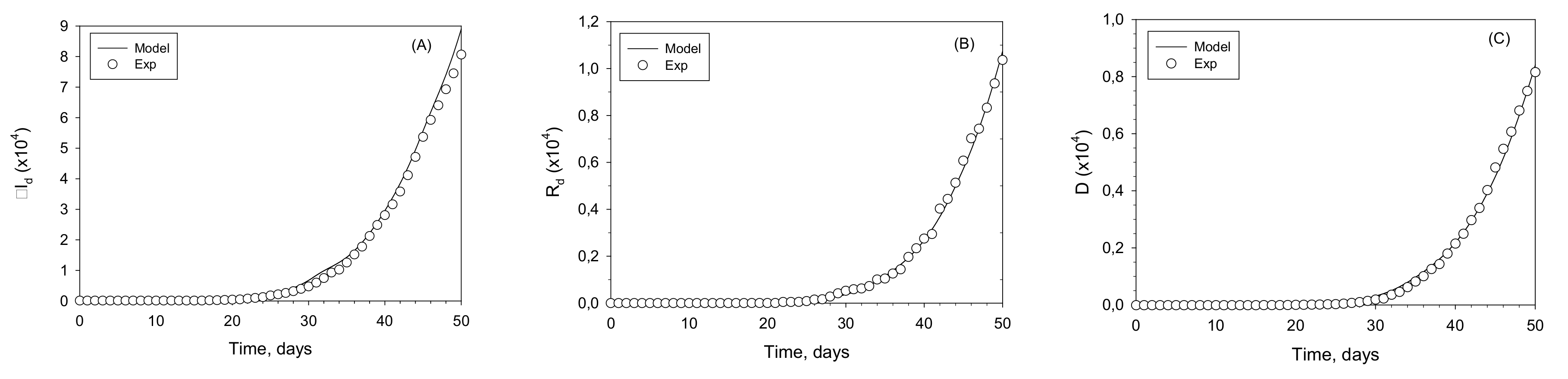
The fitting of the model to the experimental data of ΣId, Rd and D is displayed in Figure 3; the fit is satisfactory (RRMSE = 0.0461). A was not taken as an input but as an output, to avoid the uncertainty in the reported data. This is related to the lack of homogeneity in medical criteria and the availability of hospital beds and medical devices in different locations. This fit renders the numerical values for the parameters shown in Table 1. Of special interest is the mean residence time of an I patient, tr = 12.2 days and the fraction of undetected infected individuals, ϕ = 0.543. Both these values are within range of the reports available from multiple sources and strengthen the validity of our obtained results.
4. Model Behavior
In this section, we present numerical simulations that assess various characteristics of this model represented by the set of delay differential (DDE) and algebraic equations numbered from (1) to (24). To that end, all the fitted parameters listed in Table 1 were kept constant, except KSI to reveal its relative influence. This parameter is crucial in any model for the spread of COVID-19 because it characterizes the infectivity power of the virus. The simulations were run of our model extended to 200 days for four KSI values. The effect of the constant KSI on the predictions of all the variables (S, Id, Ind, A, D, Rd and Rnd) is presented in Figure 4.
These plots include the time ranges and the field data used for the fittings, but should not be considered as extrapolations, rather as extensions of their ranges, for the purpose of qualitatively exploring the potential of our model. The constants in Table 1 are strictly valid for the time ranges on which they were based. For a more accurate simulation, research based on much more data over a longer time period should be carried out; such a study is currently beyond our means. The primary purpose of this study is to present our novel conceptual approach.
The constant, KSI, which may be seen as an infectivity coefficient in the formulation of the rate of S decrease, rSI, is one of the main factors affecting the performance of the model. Within the context of the COVID-19 pandemic, its variation range is rather limited to the altered infectivity of various the mutations. Nonetheless, a wider range of variation is shown in Figure 4, in order to display the general characteristics and the potential of extension of our model to other viruses with a similar mechanism of dissemination. The profiles of the diagnosed, infected Id, the dead D, the assisted, hospitalized A and the diagnosed, recuperated Rd are shown. Bear in mind that Id(t) is the number of instantaneous infected, and not the cumulative number that is published sometimes. The latter can be readily calculated from Id(t). As expected, the lowest values of KSI led to the failure of the virus to spread in the population. As KSI increases, a peak in Id(t) appears. The larger the KSI, the higher the peak and the earlier it appears. The peak in the curve indicates the point at which the rate of recovery that takes place after tr days; plus, the rate of transfer to pool A equals the rate of new infections. The plots of D, A and Rd concur with this behavior and follow from it. A has a shape that is similar to that of Id(t), but at a substantially lower level.
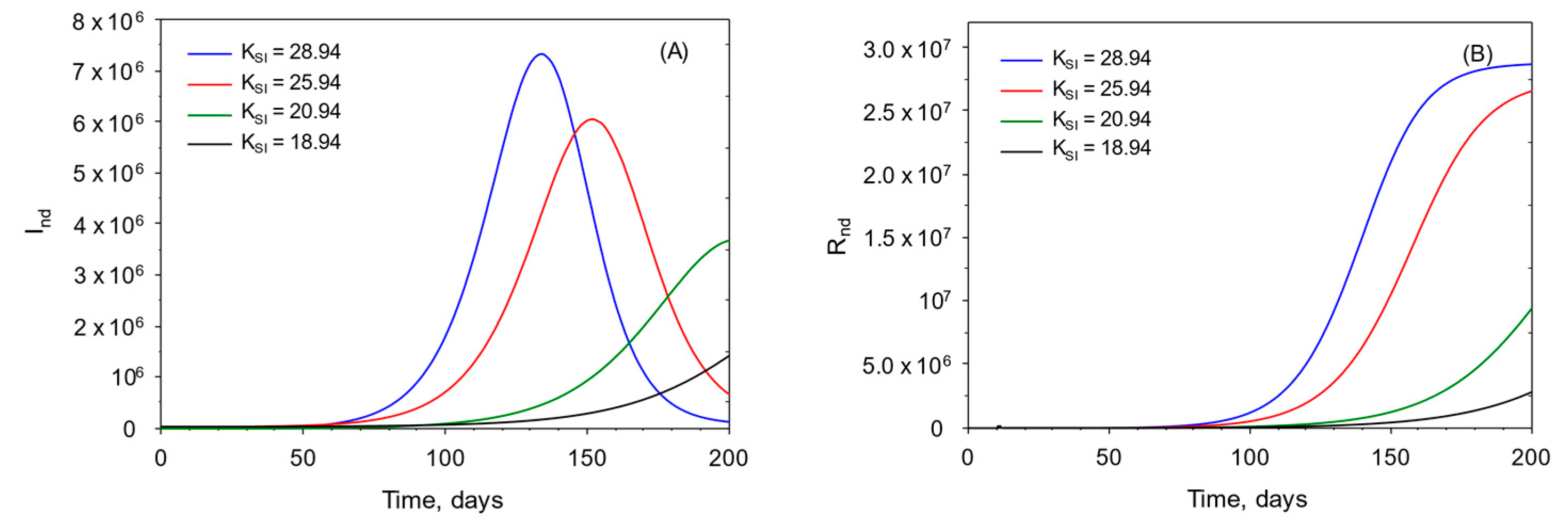
In Figure 5, the plots of the undetected infected pools Ind and Rnd are shown for the same values of KSI as in Figure 4 above. Their plots are similar to those of Id(t) and Rd(t), respectively. The calculation of those values is only possible if the knowledge of ϕ is accessible from public seroprevalence data.
5. Model Assumptions
Assumptions are one of the most substantial elements in a mathematical formulation. In the present case, the assumptions made with respect to the flow of the population in the I compartments (symptomatic and asymptomatic) are in fact its distinctive feature. Although each assumption made in the previous sections was presented next to the mathematical equation where it first appeared, most of them are collected below:
- a-
- The transit of the individuals through the I compartments is similar to a plug-flow.
- b-
- The existence of natural immunity to the virus is ignored.
- c-
- Natality is neglected.
- d-
- No mortality other that this associated to the pandemics is considered.
- e-
- No vaccination in taken into account (it would imply changes in KSI and KIdA).
- f-
- No variants of the virus are considered (it would imply changes in KSI and KIdA).
- g-
- No infected individual dies without being treated for its disease (No transit from Id directly to D).
- h-
- No age effects.
- i-
- The infection rate function ru(τ) follows the shape of Equation (1) (but other shapes may be used).
- j-
- The encounter function f(t) follows the shape of Equation (2) (but other shapes may be used).
- k-
- The the influence of the restrictions imposed on social contacts, a(t), follows the shape of Equation (3) (but other shapes may be used).
- l-
- The rate of Infection Units generation ru(τ) is the same for both detected and non-detected individuals.
All of those points above are based in common sense or on general observations of the disease characteristics but cannot be proved and remain as assumptions.
6. Preventive Quarantine
The quarantine that is usually applied in most countries as a preventive measure may be incorporated into the present model. When a patient is identified as hosting COVID-19, an epidemiologic study is carried out and all the individuals suspected of having been in potentially contagious contact with him/her are sent into quarantine, isolated for a duration that is usually less than tr. Those individuals are indicated in the integrated scheme shown in Figure 6, as pool Q. Those who test positive for COVID-19, during or at the end of the quarantine period, go to the Id pool, while the rest rejoin the susceptible in the S pool.
Strictly, those Q individuals usually enter the Id pool at a known “residence age” larger than zero; this is, however, ignored in the present version of the model for the sake of simplicity. Additionally, precise data on the number of individuals under quarantine are scant and not very reliable. Note that, here, Q is not the latent or pre-symptomatic stage that has been defined in other sources, but represents the actual quarantine as conducted in most countries. Quarantined individuals exit the S pool, at least temporarily, when joining the Q pool. The procedure of release from quarantine has several variants that may include the simple requirement of the asymptomatic passage of a certain amount of time and/or one or two negative COVID-19 tests; those testing positive enter pool Id(t), while the rest rejoin the S pool. For the present demonstration and for the sake of simplicity, we assume that the average “residence time” (tr) of an individual in pool Q (trQ), until receiving the results of the COVID-19 test from the health authorities, is 0.3·tr. We represent the number of isolated individuals per one confirmed infected by the letter w.
In order to reformulate the model to integrate pool Q, we rewrite Equations (12), (13), (23) and (24) as:
In Equation (29), the first and the second terms on the right-hand side correspond to the outputs from pool S to the two pools of infected people, Ind(t) and Id(t), respectively, as seen in Equation (23). The third term in Equation (29), represents the flux from pool S to Q, which is simply w times the flux from S(t) to Id(t). The ratio w is defined in Equation (31) below:
The fourth and fifth terms are related to the exit of individuals from pool Q. The fourth term, is the net output from pool Q to S, defined as follows:
It has been assumed that this flux is proportional to the number of individuals in isolation, Q. The term is given by:
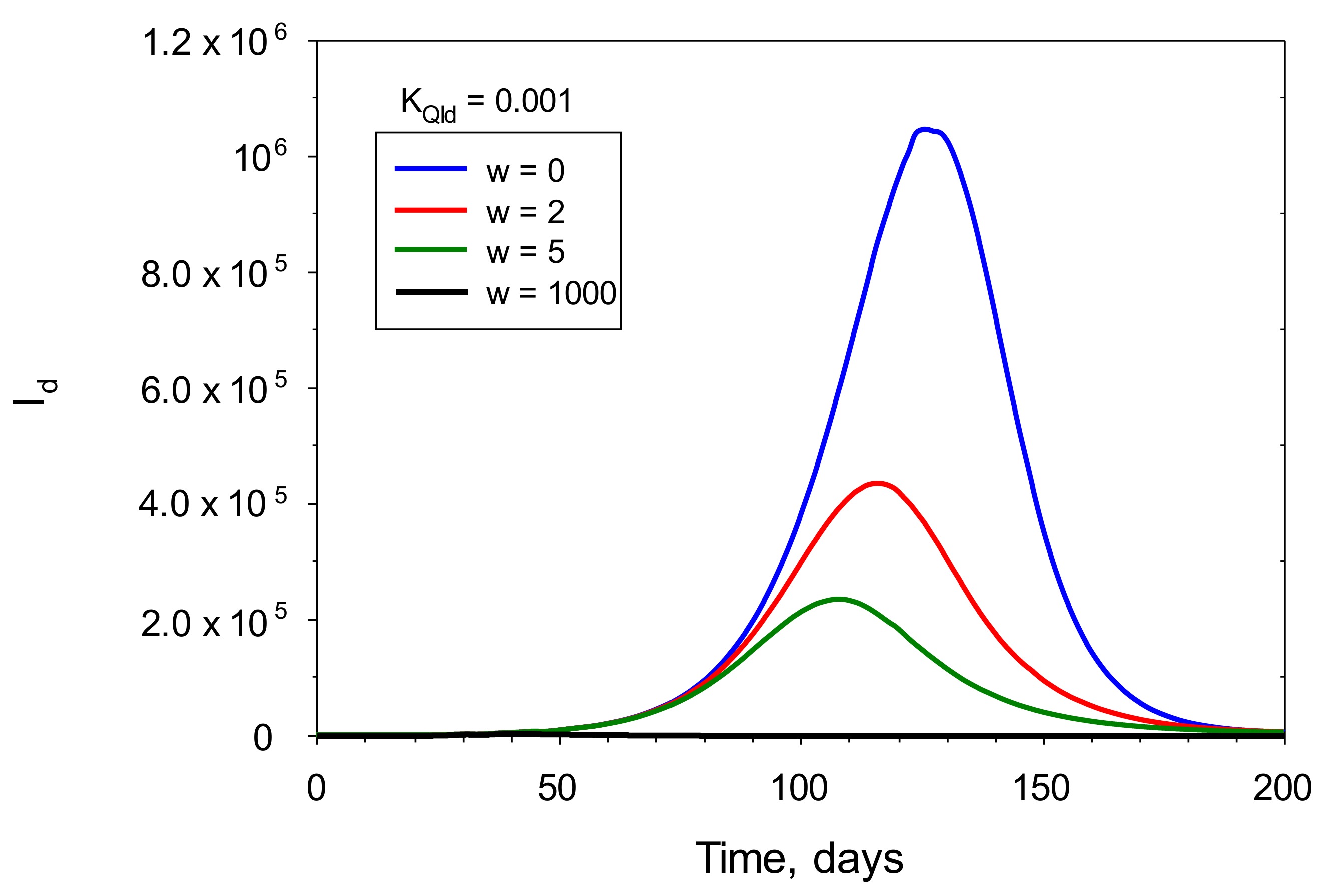
Figure 7 shows the influence of w on the Id plot for the set of parameters given in Table 1. A higher value of w indicates that more stringent preventive actions were taken. This Figure also reveals that w may have an important effect on the number of infected people. As w increases, peak value of Id decreases and appears at shorter times, that is, Id begins to decrease earlier. Thus, this model stresses the importance and effectiveness of quarantine in the management and control of the pandemics. In this sense the infection units model may become a useful tool in the planification of pandemic control preventive measures.
7. Conclusions
A novel, deterministic mathematical model of the spread of the COVID-19 virus is presented here. This model describes the mechanism of the spread of the pandemic as it has been seen in practice. It includes variables such as the number of individuals in the following pools: S (susceptible); Id (diagnosed, infected); Ind (undetected, infected); A (assisted, hospitalized); RdR (diagnosed, recuperated); RndR (undetected, recuperated); and Q (quarantined) individuals in a given population pool. The main novelty in our model are the dynamics of the disease; our model also consists of presenting of the I pool, not as a mixed compartment, but as a plug flow system, in which each of the individuals remains for a fixed period of time. In this sense the present model is conceptually different from SIRD-type models and, in fact, from most of the available deterministic models. Our model precludes the possibility that an infected patient recuperates in a time shorter than the mean infective time tr, a possibility that exist in the classic SIRD model as a consequence of the being pool of infected “perfectly mixed”. The scheme presented here is quite general and may be applied to the spread of practically any viral disease of fixed duration. It is expected that the key ideas in this model will become useful building blocks for the construction of more complex and generalized “supermodels” that should include metapopulations, agent-based elements, statistical tools, cultural and economic aspects and their influence on the spread of pandemics such as COVID-19.
Author Contributions
Conceptualization, J.C.M. and F.G.-C.; methodology, J.C.M., F.G.-C. and L.L.-R.; software, L.L.-R.; validation, L.L.-R. and F.G.-C.; formal analysis, J.C.M., F.G.-C. and L.L.-R.; investigation, J.C.M. and F.G.-C.; resources, J.C.M., F.G.-C. and L.L.-R.; data curation, F.G.-C. and L.L.-R.; writing—original draft preparation, J.C.M.; writing—review and editing, J.C.M. and F.G.-C.; visualization, F.G.-C.; supervision, J.C.M. and F.G.-C. All authors have read and agreed to the published version of the manuscript.
Funding
This research received no external funding.
Institutional Review Board Statement
Not applicable.
Informed Consent Statement
Not applicable.
Conflicts of Interest
The authors declare no conflict of interest.
Nomenclature
| A | Assisted, hospitalized individuals |
| a(t) | Function representing influence of restrictions imposed by “social distancing” on social contact (dimensionless) |
| b | Parameter in the ru equation which modulates the width of the shifted ru Gaussian curve (days) |
| D | Dead individuals |
| f | Encounter function (dimensionless) |
| fo | Coefficient in the encounter function f (dimensionless) |
| I | Infected individuals |
| Id | Detected infected individuals |
| Ind | Undetected infected individuals |
| KAD | Rate constant in rAD (day−1) |
| KARd | Rate constant in rARd (day−1) |
| KIdA | Rate constant in rIdA (day−1) |
| KIdRd | Rate constant in rIdRd (day−1) |
| KQId | Rate constant in rQId (day−1) |
| KSI | Infectivity coefficient in rSI (infected individuals U−1) |
| P0 | Target population (individuals) |
| Q | Isolated individuals by preventive quarantine |
| R | Recovered individuals |
| rAD | Flux of individuals from pools A to D (individuals/day−1) |
| rARd | Flux of individuals from pools A to Rd (individuals/day−1) |
| Rd | Recovered individuals from pool Id (diagnosed, infected individuals) |
| rIdA | Flux of individuals from pools Id to A (individuals/day−1) |
| rIdRd | Flux of individuals from pools Id to Rd (individuals/day−1) |
| rIndRnd | Flux of individuals from pools Ind to Rnd (individuals/day−1) |
| Rnd | Recovered individuals from pool Ind (undetected, infected individuals) |
| rQId | Flux of individuals from pools Q to Id (individuals/day−1) |
| rQS | Flux of individuals from pools Q to S (individuals/day−1) |
| rSI | Flux of individuals from pools S to I (individuals/day−1) |
| rSid | Flux of individuals from pools S to Id (individuals/day−1) |
| rSind | Flux of individuals from pools S to Ind (individuals/day−1) |
| rSQ | Flux of individuals from pools S to Q (individuals/day−1) |
| ru | Individual infectivity of an infected person (U/day−1/individual−1) |
| rumax | Maximum value of the ru equation (=1) (U day−1 individual−1) |
| S | Susceptible individuals |
| t | Time (day) |
| tc | Starting time of restriction implementation by authorities (day) |
| tr | Average “residence time”/”age” in the I pool (day) |
| trQ | Average “residence time”/”age” in the Q pool (day) |
| U | Infection units (dimensionless) |
| Greek letters | |
| w | Mean number of isolated individuals per each confirmed infected individual |
| βf | The limit value towards which a(t) tends (dimensionless) |
| βo | The starting value of the function a(t) (dimensionless) |
| λ | Decay rate of social contact (day−1) |
| τ | Dimensionless residence time, tr, defined in the I pool (-) |
| τIdA | Typical age of the patient passing from pool Id to that pool A (-) |
| τmax | Point in τ where rumax is reached in the ru equation (-) |
| τmix | Point in τ where rumin is reached in the ru equation (-) |
| ϕ | Fraction of infected individuals (I) that were undetected, Ind (dimensionless) |
| Ψ’nd | Infectivity of the Ind pool for t < tr (U day−1) |
| Ψnd | Infectivity of the Ind pool for t ≥ tr (U day−1) |
References
- Ceylan, Z. Estimation of COVID-19 prevalence in Italy, Spain, and France. Sci. Total Environ. 2020, 729, 138817. [Google Scholar] [CrossRef] [PubMed]
- Acemoglu, D.; Chernozhukov, V.; Werning, I.; Whinston, M.D. A Multi-Risk SIR Model with Optimally Targeted Lockdown; NBER Working Paper (w27102); National Bureau of Economic Research: Cambridge, MA, USA, 2020. [Google Scholar]
- Alvarez, F.E.; Argente, D.; Lippi, F. A Simple Planning Problem for Covid-19 Lockdown; National Bureau of Economic Research: Cambridge, MA, USA, 2020; pp. 0898–2937. [Google Scholar]
- Keeling, M.J.; Rohani, P. Modeling Infectious Diseases in Humans and Animals; Princeton University Press: Princeton, NJ, USA, 2007. [Google Scholar]
- Fraser, N.; Brierley, L.; Dey, G.; Polka, J.K.; Pálfy, M.; Nanni, F.; Coates, J.A. The evolving role of preprints in the dissemination of COVID-19 research and their impact on the science communication landscape. PLoS Biol. 2021, 19, e3000959. [Google Scholar] [CrossRef]
- Wu, J.T.; Leung, K.; Leung, G.M. Nowcasting and forecasting the potential domestic and international spread of the 2019-nCoV outbreak originating in Wuhan, China: A modelling study. Lancet 2020, 395, 689–697. [Google Scholar] [CrossRef] [Green Version]
- Hunter, E.; Mac Namee, B.; Kelleher, J.D. A Comparison of Agent-Based Models and Equation Based Models for Infectious Disease Epidemiology. In Proceedings of the AICS, Singapore, 6–8 June 2018; pp. 33–44. [Google Scholar]
- Tsori, Y.; Granek, R. Epidemiological model for the inhomogeneous spatial spreading of COVID-19 and other diseases. medRxiv 2020. [Google Scholar] [CrossRef] [PubMed]
- Danckwerts, P.V. Continuous flow systems: Distribution of residence times. Chem. Eng. Sci. 1953, 2, 1–13. [Google Scholar] [CrossRef]
- Manenti, F.; Galeazzi, A.; Bisotti, F.; Prifti, K.; Dell’Angelo, A.; Di Pretoro, A.; Ariatti, C. Analogies between SARS-CoV-2 infection dynamics and batch chemical reactor behavior. Chem. Eng. Sci. 2020, 227, 115918. [Google Scholar] [CrossRef] [PubMed]
- Cao, J.; Jiang, X.; Zhao, B. Mathematical modeling and epidemic prediction of COVID-19 and its significance to epidemic prevention and control measures. J. Biomed. Res. Innov. 2020, 1, 1–19. [Google Scholar]
- Ivorra, B.; Ferrández, M.R.; Vela-Pérez, M.; Ramos, A. Mathematical modeling of the spread of the coronavirus disease 2019 (COVID-19) taking into account the undetected infections. The case of China. Commun. Nonlinear Sci. Numer. Simul. 2020, 88, 105303. [Google Scholar] [CrossRef]
- Ivorra, B.; Ngom, D.; Ramos, Á.M. Be-codis: A mathematical model to predict the risk of human diseases spread between countries—validation and application to the 2014–2015 ebola virus disease epidemic. Bull. Math. Biol. 2015, 77, 1668–1704. [Google Scholar] [CrossRef] [PubMed] [Green Version]
- Sen, D.; Sen, D. Use of a modified SIRD model to analyze COVID-19 data. Ind. Eng. Chem. Res. 2021, 60, 4251–4260. [Google Scholar] [CrossRef]
- Bar-On, Y.M.; Flamholz, A.; Phillips, R.; Milo, R. Science Forum: SARS-CoV-2 (COVID-19) by the numbers. elife 2020, 9, e57309. [Google Scholar] [CrossRef] [PubMed]
- Linton, N.M.; Kobayashi, T.; Yang, Y.; Hayashi, K.; Akhmetzhanov, A.R.; Jung, S.M.; Yuan, B.; Kinoshita, R.; Nishiura, H. Incubation period and other epidemiological characteristics of 2019 novel coronavirus infections with right truncation: A statistical analysis of publicly available case data. J. Clin. Med. 2020, 9, 538. [Google Scholar] [CrossRef] [Green Version]
- Levenspiel, O. Chemical Reaction Engineering; Wiley Eastern Limited: New York, NY, USA, 1972. [Google Scholar]
- Liu, Y.; Gayle, A.A.; Wilder-Smith, A.; Rocklöv, J. The reproductive number of COVID-19 is higher compared to SARS coronavirus. J. Travel Med. 2020, 27, taaa021. [Google Scholar] [CrossRef] [Green Version]
- Megard, R.O.; Tonkyn, D.W.; Senft, W.H. Kinetics of oxygenic photosynthesis in planktonic algae. J. Plankton Res. 1984, 6, 325–337. [Google Scholar] [CrossRef]
- Merchuk, J.; Garcia-Camacho, F.; Molina-Grima, E. Photobioreactors–Models of Photosynthesis and Related Effects. In Comprehensive Biotechnology; Moo-Young, M., Ed.; Elsevier: Pergamon, Turkey, 2019; Volume 2, pp. 320–360. [Google Scholar]
- Prézelin, B. Light reactions in photosynthesis. In Physiological Bases of Phytoplankton Ecology; Canadian Government Publishing: Ottawa, ON, Canada, 1981; pp. 1–43. [Google Scholar]
- Zhang, Y.; Enden, G.; Wei, W.; Zhou, F.; Chen, J.; Merchuk, J.C. Baculovirus transit through insect cell membranes: A mechanistic approach. Chem. Eng. Sci. 2020, 223, 115727. [Google Scholar] [CrossRef] [PubMed]
- Backer, J.A.; Mollema, L.; Klinkenberg, D.; van der Klis, F.R.; de Melker, H.E.; van den Hof, S.; Wallinga, J. The impact of physical distancing measures against COVID-19 transmission on contacts and mixing patterns in the Netherlands: Repeated cross-sectional surveys. medRxiv 2020. [Google Scholar] [CrossRef]
- Canabarro, A.; Tenório, E.; Martins, R.; Martins, L.; Brito, S.; Chaves, R. Data-driven study of the COVID-19 pandemic via age-structured modelling and prediction of the health system failure in Brazil amid diverse intervention strategies. PLoS ONE 2020, 15, e0236310. [Google Scholar]
- Loli Piccolomini, E.; Zama, F. Monitoring Italian COVID-19 spread by a forced SEIRD model. PLoS ONE 2020, 15, e0237417. [Google Scholar]
- Prasad, J. A Data First Approach to Modelling Covid-19. medRxiv 2020. [Google Scholar] [CrossRef]
- Novack, V.; Director of Soroka Clinical Research Center Novak, Beer-Sheva, Israel. Personal Communication, 2020.
- Giordano, G.; Blanchini, F.; Bruno, R.; Colaneri, P.; Di Filippo, A.; Di Matteo, A.; Colaneri, M. Modelling the COVID-19 epidemic and implementation of population-wide interventions in Italy. Nat. Med. 2020, 26, 855–860. [Google Scholar] [CrossRef] [PubMed]
- Borchani, H.; Varando, G.; Bielza, C.; Larranaga, P. A survey on multi-output regression. Wiley Interdiscip. Rev. Data Min. Knowl. Discov. 2015, 5, 216–233. [Google Scholar] [CrossRef] [Green Version]
Figure 1.
Top: the I pool as it behaves over time, t. Bottom: the transit of a single patient through the I pool is delimited from the time of infection (inlet at τ = 0) to the end of the sickness (outlet at τ = 1).
Figure 1.
Top: the I pool as it behaves over time, t. Bottom: the transit of a single patient through the I pool is delimited from the time of infection (inlet at τ = 0) to the end of the sickness (outlet at τ = 1).

Figure 2.
Id is the pool of detected patients; Ind is the pool of non- detected individuals; Rnd includes those undiagnosed that have recuperated; Rd includes those detected and recuperated; A—the assisted, hospitalized patients; D—the dead; S—those susceptible. The broken lines indicate the action of the U that catalyze the conversion of S into I. The ri represents the flux rate between the different pools. Circles stand for mixed pools, and rectangles for plug-flow pools.

Figure 3.
Infection units model fitted to Italy: (A) cumulative detected infected population, ΣId; (B) detected, recovered population, Rd; (C) dead population, D. Experimental data (cycles); modelled populations (continuous lines).
Figure 3.
Infection units model fitted to Italy: (A) cumulative detected infected population, ΣId; (B) detected, recovered population, Rd; (C) dead population, D. Experimental data (cycles); modelled populations (continuous lines).

Figure 4.
Calculated plots of those diagnosed, infected, dead and recuperated for increasing values of the basic infectivity coefficient, KSI. (A) detected, (B) dead, (C) recovered and (D) assisted populations.
Figure 4.
Calculated plots of those diagnosed, infected, dead and recuperated for increasing values of the basic infectivity coefficient, KSI. (A) detected, (B) dead, (C) recovered and (D) assisted populations.

Figure 5.
Calculated plots of undetected, infected (A) and undetected, recuperated (B) for increasing values of the basic infectivity coefficient, KSI.
Figure 5.
Calculated plots of undetected, infected (A) and undetected, recuperated (B) for increasing values of the basic infectivity coefficient, KSI.

Figure 6.
Integrated scheme of the infection units model including the quarantine pool, Q. The main associated parameter is the number of isolated individuals per one confirmed infected, w.
Figure 6.
Integrated scheme of the infection units model including the quarantine pool, Q. The main associated parameter is the number of isolated individuals per one confirmed infected, w.

Figure 7.
Calculated plots of diagnosed, infected (Id) for increasing values of the mean number of isolated individuals per one confirmed infected (w). The simulations were performed by inserting the values of the parameters displayed in Table 1, plus the values of w and KQId that appear in the legend, into the model’s equations. KQId was fixed at 0.001.


Table 1.
Displays a summary of the parameters identified with the genetic algorithm for the early development of the COVID-19 in Italy. The range of the boundary values (low and high), initial conditions, constraints and fixed parameters during the optimization process are listed.
Table 1.
Displays a summary of the parameters identified with the genetic algorithm for the early development of the COVID-19 in Italy. The range of the boundary values (low and high), initial conditions, constraints and fixed parameters during the optimization process are listed.
| Parameter | Low | High | Fitted Value | |
|---|---|---|---|---|
| KSI | Infectivity coefficient in rSI (infected individuals U−1) | 0 | 30 | 28.950 |
| KIdRd | Rate constant in rIdRd (day−1) | 0 | 5 | 6.876 × 10⁻² |
| KIdA | Rate constant in rIdA (day−1) | 0 | 5 | 48.138 × 10⁻² |
| KARd | Rate constant in rARd (day−1) | 0 | 5 | 5.016 × 10⁻² |
| KAD | Rate constant in rAD (day−1) | 0 | 5 | 4.591 × 10⁻² |
| βfo | Coefficient in the encounter function | 0.1 | 0.8 | 26.543 × 10⁻² |
| βf1 | Coefficient in the encounter function | 0.1 | 0.8 | 13.043 × 10⁻² |
| βf2 | Coefficient in the encounter function | 0.1 | 0.8 | 12.073 × 10⁻² |
| λo | Decay rate of social contact (day−1) | 0.001 | 0.9 | 6.510 × 10⁻² |
| λ1 | Decay rate of social contact (day−1) | 0.001 | 0.9 | 7.318 × 10⁻² |
| λ2 | Decay rate of social contact (day−1) | 0.001 | 0.9 | 11.190 × 10⁻² |
| tc0 | Starting time of restriction (day) | 15 | 30 | 15.2 |
| tc1 | Starting time of (day) | 30 | 40 | 30.1 |
| tc2 | Starting time of restriction (day) | 40 | 50 | 44.8 |
| tr | Average “residence time”/”age” in the I pool (day) | 12 | 17 | 12.2 |
| τIdA | Typical infection age of the patient passing from Id to A | 0.1 | 0.9 | 0.124 |
| ϕ | Fraction of infected individuals (I) that were undetected, Ind | 0.5 | 0.9 | 0.543 |
| Constraints | ||||
| KSI > KIdA > KIdRd > KARd > KAD | βfo > βf1 > βf2 | |||
| Initial conditions | ||||
| Ind(0) = 3; Id(0) = 1; D(0) = 0; Rd(0); Rnd(0) = 0; A(0) = 0; S(0) = 59,999,996 | ||||
| Fixed parameters | ||||
| τmax = 0.5 | ||||
Publisher’s Note: MDPI stays neutral with regard to jurisdictional claims in published maps and institutional affiliations. |
© 2021 by the authors. Licensee MDPI, Basel, Switzerland. This article is an open access article distributed under the terms and conditions of the Creative Commons Attribution (CC BY) license (https://creativecommons.org/licenses/by/4.0/).
Share and Cite
MDPI and ACS Style
Merchuk, J.C.; García-Camacho, F.; López-Rosales, L. Infection Units: A Novel Approach for Modeling COVID-19 Spread. Processes 2021, 9, 2272. https://0-doi-org.brum.beds.ac.uk/10.3390/pr9122272
AMA Style
Merchuk JC, García-Camacho F, López-Rosales L. Infection Units: A Novel Approach for Modeling COVID-19 Spread. Processes. 2021; 9(12):2272. https://0-doi-org.brum.beds.ac.uk/10.3390/pr9122272
Chicago/Turabian StyleMerchuk, Jose C., Francisco García-Camacho, and Lorenzo López-Rosales. 2021. "Infection Units: A Novel Approach for Modeling COVID-19 Spread" Processes 9, no. 12: 2272. https://0-doi-org.brum.beds.ac.uk/10.3390/pr9122272
Note that from the first issue of 2016, this journal uses article numbers instead of page numbers. See further details here.