
Migration-Based Moth-Flame Optimization Algorithm
by
 , , , , and
Mohammad H. Nadimi-Shahraki
1,2,* ,
,
Ali Fatahi
1,2 ,
,
Hoda Zamani
1,2 ,
,
Seyedali Mirjalili
3,4,* ,
,
Laith Abualigah
5,6 and
and
Mohamed Abd Elaziz
7,8,9,10
1
Faculty of Computer Engineering, Najafabad Branch, Islamic Azad University, Najafabad 8514143131, Iran
2
Big Data Research Center, Najafabad Branch, Islamic Azad University, Najafabad 8514143131, Iran
3
Centre for Artificial Intelligence Research and Optimisation, Torrens University Australia, Brisbane 4006, Australia
4
Yonsei Frontier Lab, Yonsei University, Seoul 03722, Korea
5
Faculty of Computer Sciences and Informatics, Amman Arab University, Amman 11953, Jordan
6
School of Computer Sciences, University Sains Malaysia, Pulau Pinang 11800, Malaysia
7
Department of Mathematics, Faculty of Science, Zagazig University, Zagazig 44519, Egypt
8
Artificial Intelligence Research Center (AIRC), Ajman University, Ajman 346, United Arab Emirates
9
Department of Artificial Intelligence Science & Engineering, Galala University, Suze 435611, Egypt
10
School of Computer Science and Robotics, Tomsk Polytechnic University, 634050 Tomsk, Russia
*
Authors to whom correspondence should be addressed.
Processes 2021, 9(12), 2276; https://0-doi-org.brum.beds.ac.uk/10.3390/pr9122276
Submission received: 18 November 2021
/
Revised: 6 December 2021
/
Accepted: 14 December 2021
/
Published: 18 December 2021
(This article belongs to the Special Issue Evolutionary Process for Engineering Optimization)
Abstract
:Moth–flame optimization (MFO) is a prominent swarm intelligence algorithm that demonstrates sufficient efficiency in tackling various optimization tasks. However, MFO cannot provide competitive results for complex optimization problems. The algorithm sinks into the local optimum due to the rapid dropping of population diversity and poor exploration. Hence, in this article, a migration-based moth–flame optimization (M-MFO) algorithm is proposed to address the mentioned issues. In M-MFO, the main focus is on improving the position of unlucky moths by migrating them stochastically in the early iterations using a random migration (RM) operator, maintaining the solution diversification by storing new qualified solutions separately in a guiding archive, and, finally, exploiting around the positions saved in the guiding archive using a guided migration (GM) operator. The dimensionally aware switch between these two operators guarantees the convergence of the population toward the promising zones. The proposed M-MFO was evaluated on the CEC 2018 benchmark suite on dimension 30 and compared against seven well-known variants of MFO, including LMFO, WCMFO, CMFO, CLSGMFO, LGCMFO, SMFO, and ODSFMFO. Then, the top four latest high-performing variants were considered for the main experiments with different dimensions, 30, 50, and 100. The experimental evaluations proved that the M-MFO provides sufficient exploration ability and population diversity maintenance by employing migration strategy and guiding archive. In addition, the statistical results analyzed by the Friedman test proved that the M-MFO demonstrates competitive performance compared to the contender algorithms used in the experiments.
1. Introduction
During past decades, optimization techniques have been developed widely to solve complex problems that emerged in different fields of science, such as engineering [1,2,3,4,5,6,7,8,9], clustering [10,11,12,13,14,15,16,17,18], feature selection [19,20,21,22,23,24,25,26,27,28], and task scheduling [29,30,31,32]. Such optimization problems mainly involve characteristics such as linear/non-linear constraints, non-differentiable functions, and a substantial number of decision variables. These characteristics make optimization problems almost impossible to solve by exact methods reasonably, and an effective approach is needed to tackle such complexities. Approximate algorithms are recognized as an effective approach for solving issues due to their stochastic techniques and global and local search strategies. Although metaheuristic algorithms cannot guarantee the optimality of their solutions, they can offer near-optimal solutions in a reasonable amount of time, which helps solve real-world problems [33,34,35,36,37].
Metaheuristic algorithms mostly employ stochastic techniques to solve optimization problems by exploring the search space to promote population diversity in the early iterations. In the exploitation phase, the algorithm locally searches the promising areas to enhance the quality of solutions discovered in the exploration phase. Striking a proper balance between these two tendencies leads the algorithm toward the global optimum after a limited number of iterations. The bio-inspired algorithms are the primary approach to solve optimization problems by employing biological concepts. In the literature, some of the bio-inspired algorithms, such as genetic algorithm (GA) [38], differential evolution (DE) [39], particle swarm optimization (PSO) [40], and artificial bee colony (ABC) [41], have been used to find the optimum of optimization problems in polynomial time. Although the mentioned algorithms demonstrate satisfactory results for many problems, no single metaheuristic can solve all optimization issues based on the no free lunch (NFL) theorem [42]. The NFL is the main reason for continuous developments in the field of optimization. As a result, numerous bio-inspired algorithms have been developed by introducing novel methods.
To comprehensively investigate the bio-inspired algorithms, we can classify them based on their source of inspiration to evolutionary and swarm intelligence (SI) [43]. The natural biological evolution, reproduction, mutation, and Darwin’s theory of evolution are the most used fundamentals for developing evolutionary optimization algorithms. Genetic algorithm (GA) [44], genetic programming (GP) [45], differential evolution (DE) [39], evolution strategy (ES) [46], and, from recent studies, quantum-based avian navigation optimizer algorithm (QANA) [47] are some evolutionary algorithms. During past years, many variants have been developed to improve the performance of evolutionary algorithms, such as enhanced genetic algorithm (EGA) [48], an ensemble of mutation strategies and control parameters with the DE (EPSDE) [49], the real-coded genetic algorithm using a directional crossover operator (RGA-DX) [50], and an effective multi-trial vector-based differential evolution (MTDE) [51].
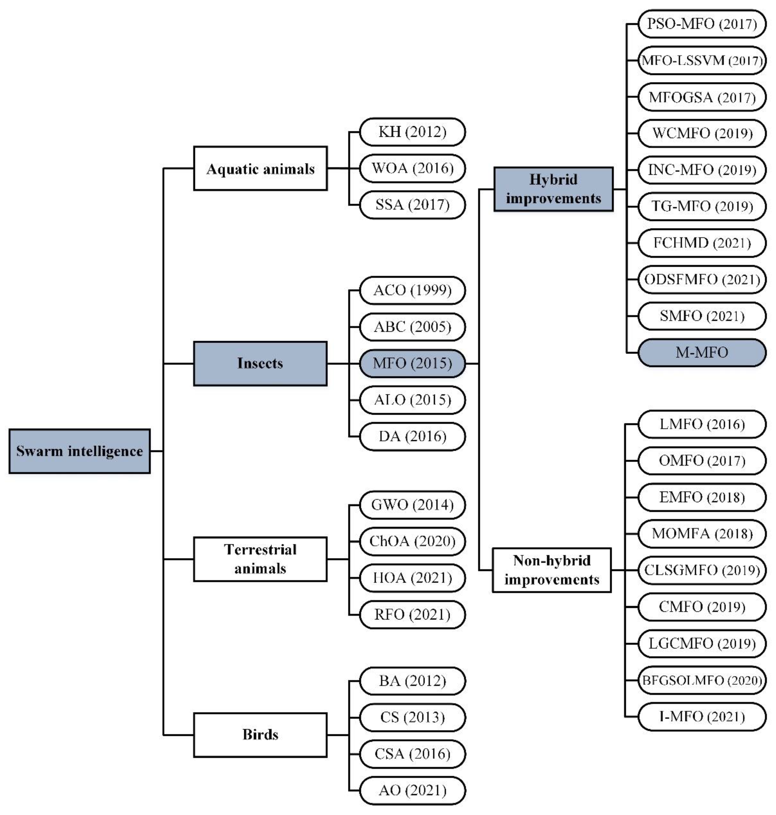
Swarm intelligence (SI) algorithms are grounded in the collective behavior of a group of biological organisms. SI algorithms can be divided into four categories: aquatic animals, terrestrial animals, birds, and insects [52]. The natural behavior of aquatic animals, such as prey besieging and foraging, has been mimicked in many SI algorithms, including the krill herd (KH) algorithm [53], whale optimization algorithm (WOA) [54], and salp swarm algorithm (SSA) [55]. Many researchers have simulated the biological behavior of terrestrial animals to propose functional metaheuristic algorithms, such as grey wolf optimizer (GWO) [41], red fox optimization algorithm (RFO) [56], chimp optimization algorithm (ChOA) [57], and horse herd optimization algorithm (HOA) [58]. In the third category, bat algorithm (BA) [59], cuckoo search algorithm (CS) [60], crow search algorithm (CSA) [61], and Aquila optimizer (AO) [62] are among the well-known algorithms inspired by birds’ behaviors. Social behaviors of insects, such as self-organization and cooperation, are the main sources of inspiration behind the fourth group of SI algorithms, including ant colony optimization (ACO) [63], artificial bee colony (ABC) [64], ant lion optimization (ALO) [65], dragonfly algorithm (DA) [66], and moth–flame optimization (MFO) [67].
The SI algorithms intrinsically benefit from autonomy, adaptability, and acceptable time complexity. However, loss of population diversity and sinking into the local optimum are common issues among most SI algorithms. Therefore, many variants have been proposed to address these shortcomings and enhance the performance of the algorithms. Karaboga et al. [68] introduced a quick artificial bee colony (qABC) algorithm to improve the exploitation ability of the traditional algorithm. The conscious neighborhood-based crow search algorithm (CCSA) [52] addresses the imbalance between exploration and exploitation. An improved grey wolf optimizer (I-GWO) [69] was proposed to maintain the population diversity. An enhanced chimp optimization algorithm (EChOA) [70] has been introduced to avoid local optimum.
The moth–flame optimization (MFO) is a prominent bio-inspired metaheuristic algorithm inspired by the moths’ spiral movement around the light source at night. The MFO algorithm stands out among many metaheuristic algorithms for its simplicity and acceptable time complexity. Therefore, the MFO is used for solving a broad range of real-world problems, such as clustering [71,72,73,74,75,76,77], feature selection [78,79,80,81,82,83,84,85], and image processing [86,87,88,89,90,91]. Although the MFO is applicable for solving real-world problems and many improvements have been developed, it has been observed that the MFO and its variants hereditarily suffer from poor exploration and loss of population diversity before the near-optimal solution is met, which leads the algorithm toward local optima trapping and premature convergence.
In this study, an enhanced MFO algorithm, named migration-based moth–flame optimization (M-MFO) algorithm, is proposed to cope with these weaknesses. The M-MFO introduces a guiding archive to maintain the population diversity and a hybrid simple strategy named migration strategy consists of two random migration (RM) and guided migration (GM) operators which take advantage of an adapted crossover introduced in the GA [44]. The RM operator is introduced to enhance the exploration ability and population diversity by crossing the unlucky moths with a randomly generated moth to migrate to new areas. If the migrated moths obtain better positions, they are updated and added to the guiding archive to guide other unlucky moths. When the guiding archive size reaches the size of the problem variables, the archive is mature enough to guide other unlucky moths using the GM operator. This dimensionally aware switch between operators can guarantee the convergence of the algorithm toward promising areas.
To evaluate the efficiency of the M-MFO, the CEC 2018 benchmark functions were conducted to investigate the characteristics and performance of the proposed algorithm and its competitors in different dimensions, 30, 50, and 100. The convergence curves and population diversity provided in Section 5, show that the M-MFO can maintain population diversity until the optimal solution emerges and effectively facilitates the convergence behavior. Moreover, the Friedman test was conducted to evaluate the obtained results statistically. The experimental and statistical results were first compared with seven well-known variants of MFO, including LMFO [92], WCMFO [93], CMFO [94], CLSGMFO [95], LGCMFO [96], SMFO [97], and ODSFMFO [98] in dimension 30. Then, the top four algorithms and eight other state-of-the-art swarm intelligence algorithms were considered for the main experiments. Hence, the total competitors for the main experiments were KH [53], GWO [41], MFO [67], WOA [54], WCMFO [93], CMFO [94], HGSO [99], RGA-DX [50], ChOA [57], AOA [100], and ODSFMFO [98]. The experimental evaluations and statistical tests revealed that the M-MFO algorithm outperforms other competitor algorithms with overall effectiveness of 91%. The experimental results revealed that the migration strategy enhances the exploration ability and maintains the population diversity to avoid local optimum by stochastically migrating the worst individuals across the search space in the first iterations and exploiting promising areas discovered by the RM operator in the next iterations. The main contributions of this study are summarized as follows.
- Introducing a guiding archive for storing improved moths to guide other unlucky moths.
- Introducing a migration strategy using RM and GM operators to improve unlucky moths.
- The RM operator enhances the exploration ability, while the GM operator converges the population toward the promising areas by exploiting around improved moths.
- The experiments prove that the M-MFO effectively maintains the population diversity by taking advantage of the guiding archive.
- The Friedman test demonstrated that the M-MFO provides the best results compared to competitors and stands out among MFO variants for solving global optimization problems.
The remainder of the paper is organized as follows. A literature overview of the MFO variants is included in Section 2. Section 3 briefly presents the MFO algorithm. Section 4 comprehensively presents the proposed M-MFO algorithm. A rigorous examination of the effectiveness of the proposed algorithm is provided experimentally in Section 5 and statistically in Section 6. Finally, Section 7 summarizes the conclusions.
2. Related Work
The MFO algorithm is known as a prominent problem solver due to its simple framework, fewer control parameters, and ease of implementation. However, the MFO suffers from some issues for solving complex optimization problems. Therefore, since the release of the MFO, many variants have been developed to address MFO’s shortcomings and offer improved performance. These variants can be categorized into hybrid improvements and non-hybrid improvements, as illustrated in Figure 1.
Since the introduction of MFO, many researchers have proposed hybrid variants to effectively address shortcomings of the canonical MFO by employing operators of other algorithms. Bhesdadiya et al. [101] introduced a hybrid PSO-MFO algorithm by combining particle swarm optimization (PSO) with MFO to boost the exploitation ability of the MFO algorithm. MFO-LSSVM [102] is a hybridization of MFO with least squares support vector machines (LSSVM) to enhance the generalization in the prediction of the MFO algorithm. To boost the exploitation ability of the MFO, Sarma et al. [103] introduced the gravitational search algorithm (GSA) to the canonical MFO and proposed MFOGSA. In WCMFO, Khalilpourazari et al. [93] introduced a combined MFO, water cycle algorithm (WCA) and a random walk to avoid local optimum and enhance the solution quality. Rezk et al. [104] designed a hybrid MPPT method by combining an incremental conductance (INC) approach and MFO, called (INC-MFO), to reach a maximum-power solar PV/thermoelectric system under different environmental conditions.
Ullah et al. [105] introduced a time-constrained genetic moth–flame optimization (TG-MFO) algorithm for an energy management system (EMS) in smart homes and buildings. The FCHMD [106] algorithm combines Harris hawks optimizer (HHO) and MFO to cope with the insufficient exploitation and exploration rate of the HHO and MFO, respectively. Moreover, the method of evolutionary population dynamics (EPD) is employed to address premature convergence and local optima stagnation. ODSFMFO, proposed by Li et al. [98], is a hybridization of MFO with differential evolution (DE) and shuffled frog leaping algorithm (SFLA). In addition, the algorithm is enhanced by the addition of a flame generation strategy and death mechanism. Dang et al. [107] brought up a hybridization of MFO and three different methods, including the Taguchi method, fuzzy logic, and response surface method, to solve the flexure hinge design problem. SMFO has been recently proposed by [97] to enhance the solution quality and convergence speed of the MFO by introducing the sine cosine strategy to the MFO algorithm.
The non-hybrid algorithms are mostly developed to cope with issues such as local optima trapping, premature convergence, the imbalance between search strategies, and poor local and global search abilities. The LMFO algorithm proposed by Li et al. [92] is an enhanced version of MFO, improved by Lévy flight to address premature convergence and local optimum trapping by improving the population diversity. Apinantanakon et al. [108] established an opposition-based moth–flame optimization (OMFO) algorithm to evade local optimum by boosting the exploration ability of the MFO. Xu et al. [109] addressed the MFO’s low population diversity and introduced EMFO by taking advantage of the Gaussian mutation (GM). Li et al. [110] presented a multi-objective moth–flame optimization algorithm (MOMFA) to enhance water resource efficiency by maintaining population diversity and accelerating convergence speed by taking advantage of opposition-based learning and indicator-based learning selection-efficient mechanisms.
The CLSGMFO [95] presents an efficient chaotic mutative moth–flame-inspired algorithm by employing Gaussian mutation and chaotic local search to enhance the population diversity and exploitation rate, respectively. Chaos-enhanced moth–flame optimization (CMFO), proposed by Hongwei et al. [94], is an improved MFO algorithm that employs ten chaotic maps. Xu et al. [96] developed LGCMFO to enhance the global and local search ability of the MFO and avoid local optimum by employing new operators, such as Gaussian mutation (GM), Lévy mutation (LM), and Cauchy mutation (CM). In BFGSOLMFO, Zhang et al. [111] introduced orthogonal learning (OL) and Broyden–Fletcher–Goldfarb–Shanno (BFGS) to the MFO to enhance the solution quality of the MFO. Nadimi-Shahraki et al. [112] proposed an improved moth–flame optimization (I-MFO) algorithm to evade the local optima trapping and premature convergence by adding a memory mechanism and taking advantage of the adapted wandering around search (AWAS) strategy. This algorithm is designed to solve the numerical and mechanical engineering problems.
3. Moth–Flame Optimization (MFO) Algorithm
The moth–flame optimization (MFO) is a prominent SI algorithm inspired by the spiral locomotion behavior of moths around a light source at night. This behavior is derived from the navigation mechanism of moths that is used to fly a long distance in a straight line by maintaining a fixed inclination to the moon. However, this principled navigation mechanism turns into a deadly spiral path toward the light source if the light source is relatively close to the moths. According to the brief description, the MFO algorithm consists of moths and flames. As shown in Equation (1), moths are considered search agents, organized in matrix M (t), that explore the D-dimensional search space, and N is the number of moths.
Additionally, the fitness of the corresponding moth is stored in an array OM (t), as shown below.
On the other hand, flames are the best positions discovered by moths and are stored in a similar matrix F (t), along with their fitness values in an array OF (t). The moths spirally move around their corresponding flames, as shown in Equation (3), where Mi (t) is the position of ith moth in the current iteration, the Disi determines the distance between Mi and its corresponding jth flame (Fj) formulated in Equation (4), b indicates the shape of the logarithmic spiral, and k is a random number value between intervals [−1, 1].
To converge the algorithm and provide more exploitation, the number of flames decreases in the course of iterations based on Equation (5), where t determines the current number of iterations, while N and MaxIt demonstrate the total number of flames and the maximum number of iterations, respectively.
4. Proposed Algorithm
The MFO is a prominent population-based algorithm that is successfully applied in different fields. However, based on the conducted analysis reported in Section 5.2 and related studies [113,114,115], the MFO algorithm suffers from poor exploration and rapid loss of population diversity. While the number of flames converges, the algorithm provides more local searches throughout the course of the iterations. Hence, the algorithm is prone to sink into the local optimum due to its limited simple spiral movement of moths around their corresponding flames which cannot offer further exploration to avoid the local optimum. Therefore, this study proposes a migration-based moth–flame optimization (M-MFO) algorithm, which is a hybridization of the MFO algorithm and the crossover operator introduced in the GA. Moreover, the M-MFO utilizes a guiding archive to maintain population diversity and a migration strategy that uses the crossover operator to boost exploration ability. The migration strategy introduces two operators, RM and GM, by taking advantage of an adapted GA’s crossover. The RM operator is introduced to provide sufficient exploration ability during the early iterations, while the GM operator converges the population toward promising areas. Moreover, to maintain the population diversity, a guiding archive is introduced, as outlined in Definition 1, to store lucky moths that have improved using the migration strategy.
Definition 1 (guiding archive).
The guiding archive keeps the position of lucky moths improved by the migration strategy to maintain the population diversity and suppress the premature convergence of the population. Both RM and GM add improved moths to the guiding archive, although only the GM operator exploits the archive. The guiding archive capacity (MaxArc) is formulated in Equation (6), where D and N are dimensions and population size.
To ensure that the guiding archive is mature enough to guide other unlucky moths, the current size of the archive (δ) needs to be greater than the size of the problem variables (D). This limitation provides a dimensionally aware switch to choose the right operator in the migration strategy effectively. In addition, if the value of δ exceeds the MaxArc, the next moth is replaced with a random member of the guiding archive.
Migration strategy includes RM and GM operators to ensure that there is high enough exploration capability and convergence toward promising zones. The RM operator provides further exploration ability by changing the position of Mi stochastically. At the same time, the GM operator is introduced to converge the population toward promising zones by exploiting improved moths kept in the guiding archive. Moreover, the migration strategy benefits from a dimensionally aware switch between these two operators as represented in Equation (7), where δ indicates the current size of the guiding archive. The pseudo-code and the flowchart of the M-MFO are presented in Algorithm 1 and Figure 2, respectively.
Random migration (RM) operator: Let unlucky moths (t) = {M1, M2, …, Mi, …}, which is a finite set of unlucky moths, such that OMi (t) > OMi (t − 1). Hence, in this operator, the position of Mi changes by considering a randomly generated moth (Mr) and Mi represents the parents in the crossover formulated in Equations (8) and (9), where α is a random number in [0, 1]. The crossover produces two offspring, and the one with better fitness is selected and compared with other offspring to choose the best one, and the position of OMi (t + 1) is added to the guiding archive if it can dominate the OMi (t). The RM operator satisfies the need for exploration by stochastically moving the unlucky moths to discover promising areas in the early iterations.
Guided migration (GM) operator: The GM operator is employed to change the position of unlucky moth, Mi, when the size of the GM reaches the size of the problem variables. The GM changes the position of Mi by employing the crossover formulated in Equations (10) and (11), where LMr is a random lucky moth from the guiding archive. Similarly, to the RM operator, if the new offspring obtains a better position compared to Mi (t), the position of Mi (t + 1) is updated, and it is appended to the guiding archive.
| Algorithm 1. The pseudocode of proposed M-MFO algorithm. | |
| Input: Max iterations (MaxIt), number of moths (N), max size of guiding archive (MaxArc), and dimension (D). | |
| Output: The best flame position and its fitness value. | |
| Begin | |
| Randomly distributing M moths in the D-dimensional search space. | |
| Calculating moths’ fitness (OM). | |
| Set t and δ = 1 //δ is the number of guiding archive members. | |
| OF (t) ← sort OM (t). | |
| F (t) ← sort M (t). | |
| While t ≤ MaxIt | |
| Updating F and OF by the best N moths from F and current M. | |
| Updating FlameNum (t) using Equation (5). | |
| For i = 1: N | |
| Updating the position of Mi (t) using Equation (3) and computing the OMi (t). | |
| If OMi (t) > OMi (t − 1) | |
| τ ← Generating a random number between intervals [1, D]. | |
| For j = 1: τ | |
| If δ ≤ D (The guiding archive is still immature) | |
| Generating the next position Mi (t + 1) using RM operator and Equations (8) and (9). | |
| Else (The guiding archive is mature) | |
| Generating next position Mi (t + 1) using GM operator and Equations (10) and (11). | |
| End If | |
| End For | |
| If OMi (t + 1) < OMi (t) | |
| Updating position Mi (t) and adding Mi (t + 1) to guiding archive using Definition 1 and MaxArc. | |
| End If | |
| End If | |
| End For | |
| Updating the position and fitness value of the global best flame. | |
| t = t +1. | |
| End while | |
5. Numerical Experiment and Analysis
In this section, the performance of the proposed M-MFO has been evaluated on several benchmark functions. In the first section, the population diversity and convergence behavior of the canonical MFO have been analyzed on some selected functions to provide some useful information about the shortcomings of the MFO algorithm. Then, the MFO variants and the M-MFO have been compared on dimension 30 to determine the top four superior MFO variants to participate in the next experiments. Following that, the performance of M-MFO has been compared with ten of the state-of-the-art swarm intelligence algorithms: KH [53], GWO [41], MFO [67], WOA [54], WCMFO [93], CMFO [94], HGSO [99], RGA-DX [50], ChOA [57], AOA [100], and ODSFMFO [98]. The parameters of the competitor algorithms are reported in Table 1.
5.1. Experimental Environment and Benchmark Functions
The M-MFO and competitor algorithms were implemented in Matlab 2020a. All experiments were performed 20 times, independently, on a laptop with Intel Core i7-10750H CPU (2.60 GHz) and 24 GB of memory to ensure fair comparisons. In each run, the maximum number of iterations (MaxIt) was set by (D × 104)/N where D and N were respectively set to the dimensions of the problem and 100. In this study, the CEC 2018 benchmark functions [116] were used to evaluate the effectiveness of the proposed M-MFO. There are 29 test functions in the CEC 2018 benchmark suite, each with its own set of characteristics and different dimensions 30, 50, and 100. These test functions can be classified into unimodal functions F1 and F3, multimodal functions F4–F10, hybrid functions F11–F20, and composition functions F21–F30. The experimental results tabulated in Table 2, Table 3, Table 4 and Table 5 and Table A1, Table A2, Table A3 and Table A4 in the Appendix A are based on each algorithm’s average and minimum fitness value, where the bold values illustrate the winning algorithm. Moreover, the symbols “W|T|L” in the last row of each table demonstrate the number of wins, ties, and losses for each algorithm.
5.2. Population Diversity Analysis
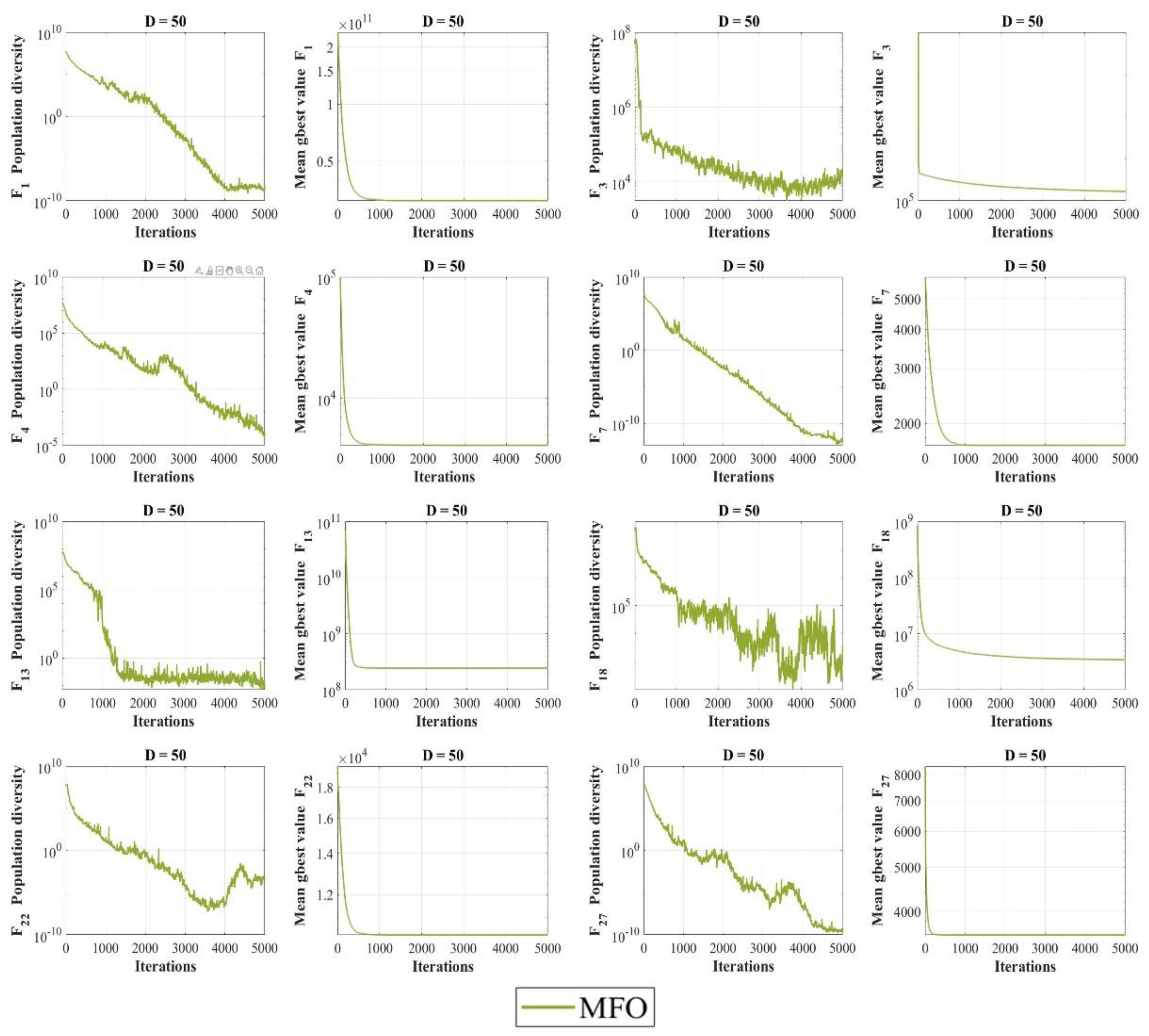
Maintaining population diversity plays a crucial role in metaheuristic algorithms during the optimization process, as low diversity among search agents can lead the algorithm toward getting stuck at a local optimum. In this experiment, the population diversity and convergence behavior of the MFO algorithm were comprehensively examined to discover the shortcomings of the MFO algorithm. The population diversity curves shown in Figure 3 were measured by a moment of inertia (Ic) [117], where the Ic represents the spreading of each individual from their centroid given by Equation (12) and the centroid cj for j = 1, 2 … D was calculated using Equation (13).
In order to perform a fair analysis and develop a better understanding of how population diversity affects the optimization process, Figure 3 illustrates the population diversity and convergence curves of the MFO side by side. For unimodal function F1, the diversity fell while the optimal solution had not been met yet. Hence, the algorithm sunk into the local optimum until the last iterations. For F3, the slope of losing diversity was not as sharp as F1, and the convergence trend continued until the last iterations. However, the population diversity was still low, and convergence speed was too slow to reach the near-optimal solution in the course of iterations. F4 and F7 represent the multimodal functions in which the MFO could not maintain the population diversity, and the algorithm experienced premature convergence, beginning at early iterations. F13, F18, F22, and F27 were plotted as representatives of hybrid and composition functions with similar diversity and convergence behaviors. The standard behavior was the effort of the algorithm to avoid the local optimum by increasing the population diversity; however, the simple movements of search agents in MFO could not satisfy the needs of exploration to escape the local optimum. To sum up, it can be concluded from the plots that the MFO loses its population diversity before reaching an optimal solution. This behavior was repeated for most of the functions, proving the deficiency of the algorithm in maintaining the population diversity.
5.3. Comparison of M-MFO with MFO Variants
To compare M-MFO with more variants, the results of M-MFO and seven other well-known variants of MFO, including LMFO [92], WCMFO [93], CMFO [94], CLSGMFO [95], LGCMFO [96], SMFO [97], and ODSFMFO [98], were assessed and tabulated in Table 2 and Table A1 in the Appendix A, where the M-MFO outperformed its competitors in dimension 30. Then, the top four algorithms, including the proposed M-MFO, ODSFMFO, WCMFO, and CMFO, were selected for main experiments, including comparison results on dimensions 30, 50, and 100; convergence analysis; population diversity analysis; and the Friedman test.
5.4. Evaluation of Exploitation and Exploration
The exploitation and exploration abilities of the proposed M-MFO have been evaluated by unimodal and multimodal test functions, respectively. As the unimodal functions, F1 and F3 have a single global optimum and they are suitable for assessing the exploitation abilities of optimization algorithms. Based on the results of the unimodal functions reported in Table 3 and Table A2 in the Appendix A, the M-MFO outperformed competitors for 30, 50, and 100 dimensions, particularly on test function F3, where the M-MFO provided the global best solution. The main reason for this exploitation ability is to employ the GM operator, which effectively exploits improved moths kept in the guiding archive. To assess the exploration ability of the M-MFO, the multimodal test functions F4–F10 were considered, as multimodal functions have many local optima. The results of multimodal test functions demonstrated that the M-MFO provides very competitive results compared to other competitors, mainly because of the RM operator and its stochastic movement employed for exploring the landscape effectively in the early iterations.
5.5. Local Optima Avoidance Analysis
In this experiment, the local optima avoidance ability and balance between exploration and exploitation of M-MFO were investigated using hybrid F11–F20 and composition F21–F30 functions with dimensions 30, 50, and 100. The related results, tabulated in Table 4, Table 5, Table A3 and Table A4 in the Appendix A, proved that the M-MFO is very competitive in comparison to other algorithms used for approximating the global optima values. The main reason is that the algorithm optimally trades off exploration and exploitation by defining two operators—the RM operator, which stochastically moves the unlucky search agents across the search space, and the GM operator, which exploits the promising areas located by successful migrants. Additionally, a guiding archive is introduced to maintain the population diversity by storing new solutions obtained by migration strategy. Moreover, defining a dimensionally aware switching between operators of migration strategy guarantees a proper trade-off between exploration and exploitation.
5.6. The Overall Effectiveness of M-MFO
This study evaluated the overall effectiveness (OE) of the M-MFO and contender algorithms based on the results reported in Table 3, Table 4 and Table 5 and Table A2, Table A3, Table A4 in Appendix A. The OE results reported in Table 6 were calculated using Equation (14), where N indicates the total number of test functions and L is the number of losing tests for each algorithm. The results prove that the M-MFO, with overall effectiveness of 91%, is the most effective algorithm for the various dimensions 30, 50, and 100.
5.7. Convergence Rate Analysis
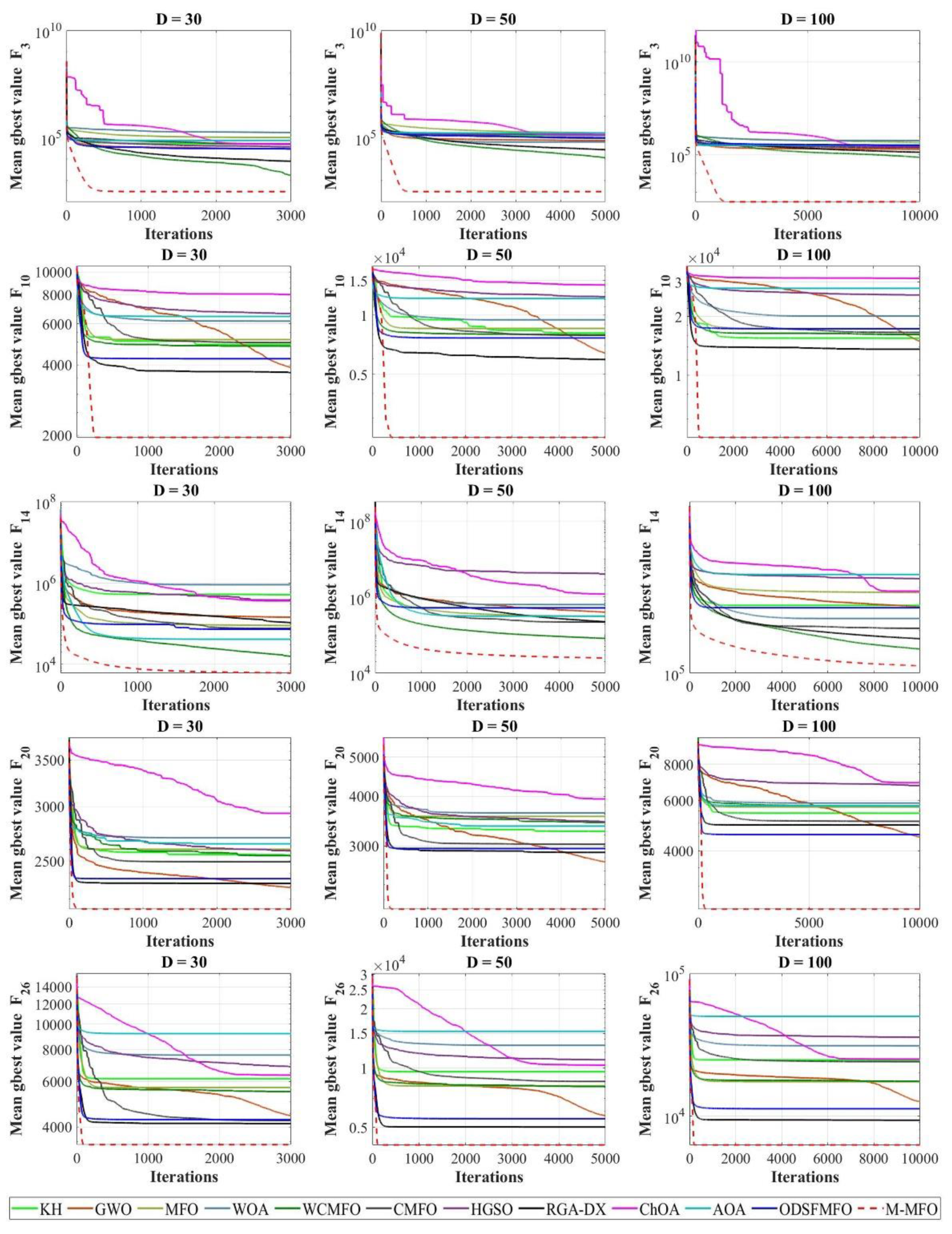
In this experiment set, the convergence properties of the M-MFO were examined and the results were compared with contender algorithms for dimensions 30, 50, and 100. Figure 4 illustrates the convergence curves of the average fitness values obtained by each algorithm on unimodal, multimodal, hybrid, and composition test functions. The first row shows the convergence behavior of algorithms on F3. The M-MFO hit the global optimum solution in the early iterations for all dimensions, which proved the sufficient exploitation ability of the M-MFO. In contrast, the convergence trends of other algorithms were hampered by local minima or demonstrated a prolonged convergence rate. For multimodal function F10, the M-MFO provided the best solution among competitors in the early iterations due to its exploration ability derived from the migration strategy. The third and fourth rows present the convergence of the hybrid functions. The M-MFO bypassed the local optima and continued its gradual trend toward the near-optimum solutions until the final iterations by striking a balance between exploration and exploitation. The convergence curves of the composition function illustrated in the last row demonstrate that the M-MFO obtained the best solution among competitors in early iterations. To sum up, the plots proved that the M-MFO is superior to the other algorithms and provides sufficient exploitation, exploration, and balance between these two tendencies. In addition, it can be noticed that the M-MFO offered more consistent results by increasing the size of the problem variables.
5.8. Population Diversity Analysis
As mentioned in Section 5.2, adequate population diversity can suspend the algorithm from local optima trapping. Therefore, in this section, the population diversity of M-MFO and other competitors is provided in Figure 5. Comparing the population diversity with convergence curves provided in the previous section demonstrated that the M-MFO effectively maintained its population diversity until the promising area was met for different test functions with dimensions of 30, 50, and 100. Furthermore, the plots suggest that the M-MFO shows strong robustness for maintaining the population diversity as the size of the problem variables increases, mainly for its dimensionally aware switch between operators.
5.9. Sensitivity Analysis on the Guiding Archive Maturity Size
As discussed in Definition 1, the M-MFO algorithm switches from RM to GM operator when the guiding archive has matured. Hence, in this experiment, the impact of considering different maturity sizes of the guiding archive was evaluated and is discussed in relation to four different scenarios. Table 7 shows the fitness values gained in each scenario among five functions (i.e., F1, F9, F17, and F30) for different dimensions 30, 50, and 100.
The reported results indicate that the fourth scenario (δ = D) among all the tested functions provided better results overall compared to other scenarios. Nevertheless, it can be noticed that other scenarios provided competitive results, especially for unimodal functions. The main reason lies behind the fact that the higher value for maturity provides more population diversity and exploration ability, while the need for exploitation ability is more highlighted for unimodal functions. Moreover, previous studies [47,52] have proved that increasing the dimension has a negative impact on the effectiveness and scalability of metaheuristic algorithms. Hence, the size of the problem variables for maturity condition (δ = D) can provide dimensional robustness for the algorithm. Furthermore, considering D as the maturity size does not add any additional parameters to the algorithm, and it provides an autotune parameter for different dimensions.
6. Statistical Analysis
In this experiment, the Friedman test [118] was conducted to statistically prove the superiority of M-MFO by ranking the algorithms based on their performance on CEC 2018 benchmark functions. Table 8 illustrates the obtained results for unimodal and multimodal test functions. In addition, hybrid and composition functions have been tabulated in Table 9. Inspecting the overall rank of the Friedman test, it is evident that the M-MFO demonstrated superior performance in comparison to contender algorithms for dimensions of 30, 50, and 100.
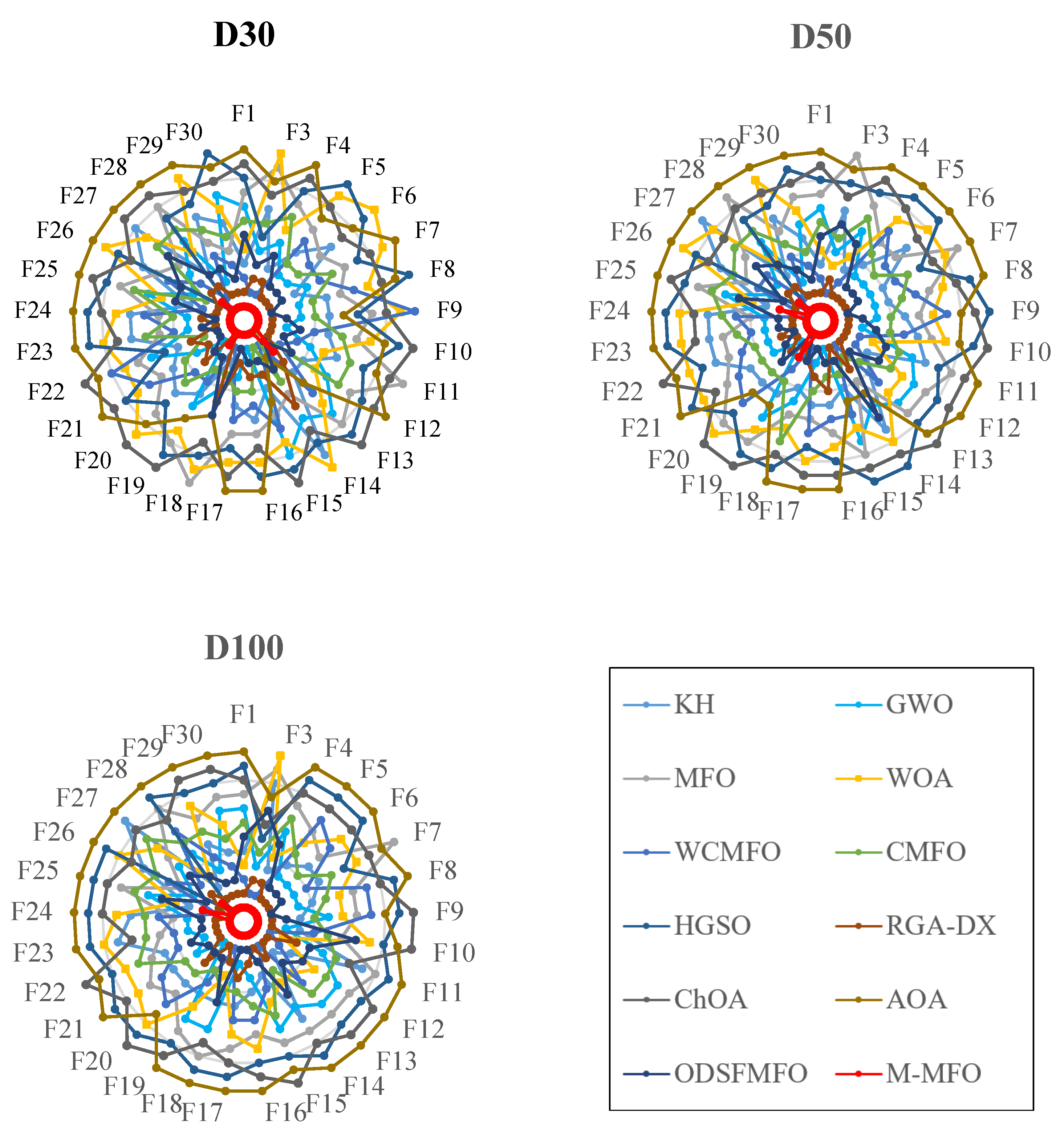
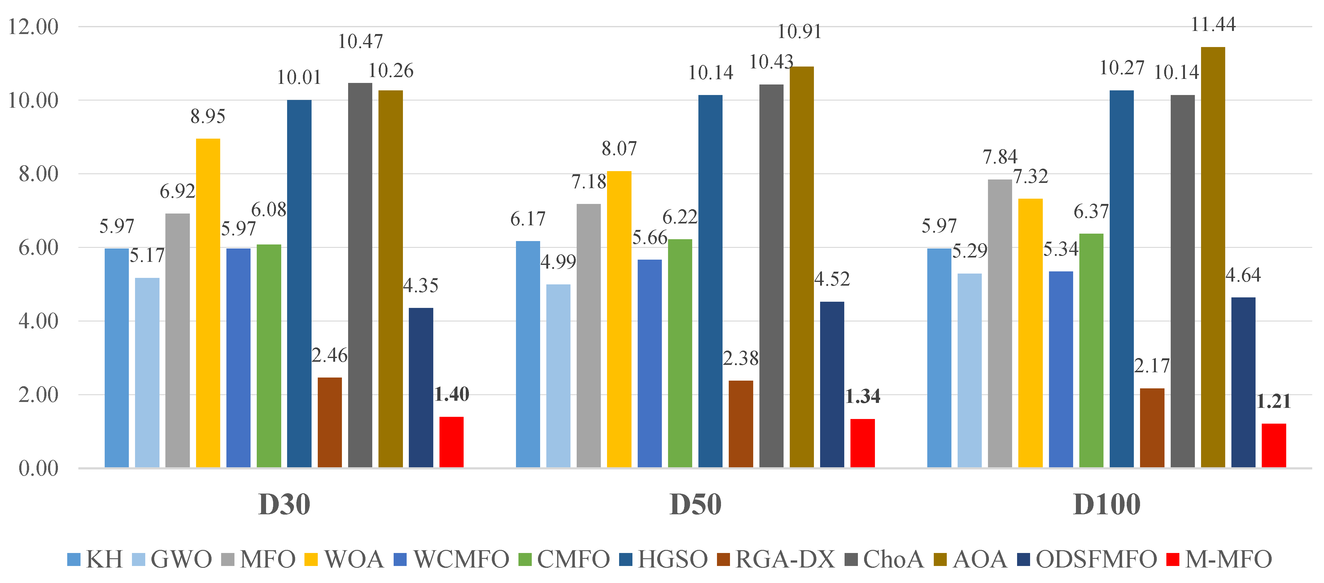
In Figure 6 and Figure 7, the M-MFO and competitors are visually ranked based on their performance in CEC 2018 benchmark suite for various dimensions. Figure 6 depicts the ranking results of algorithms in solving CEC 2018 benchmark functions, expressed through a radar graph. Meanwhile the clustered bar chart of Friedman’s test average results is shown in Figure 7. The radar graph demonstrates that the M-MFO surpassed other algorithms in the majority of test functions for various dimensions. The clustered bar chart shows that the M-MFO achieved the best rank among competitors since it has the shortest bar in the different dimensions of 30, 50, and 100.
7. Conclusions
The MFO is a successful metaheuristic algorithm inspired by moths’ behavior converging to a light source at night. The MFO has been used in various real-world optimization problems during recent years, mainly due to its simple structure. However, as the experiments revealed, the canonical MFO algorithm experiences local optima trapping and premature convergence due to the rapid dropping of population diversity and poor exploration. Hence, the M-MFO algorithm is proposed to overcome MFO’s shortcomings by introducing a migration strategy that includes two new operators to boost exploration ability and maintain the population diversity.
The performance of M-MFO was experimentally evaluated by conducting CEC 2018 benchmark functions on dimension 30 and compared with seven recent variants of MFO, including LMFO, WCMFO, CMFO, CLSGMFO, LGCMFO, SMFO, and ODSFMFO. The top four latest high-performing variants and eight other state-of-the-art swarm intelligence algorithms were considered for experiments on the 30, 50, and 100 dimensions. The M-MFO stood out among competitors by providing highly competitive results and maintaining robustness while the size of the problem variables increased. In addition, to rank the algorithms, M-MFO and competitors were analyzed statistically by the Friedman test, in which the M-MFO obtained the first rank. For future works and studies, the migration strategy and guiding archive could be considered a reference in handling low population diversity and inefficient exploration of other metaheuristic algorithms. Moreover, the M-MFO can be used to solve engineering design problems. It can be converted for solving discrete optimization problems, such as feature selection, data mining, and image segmentation.
Author Contributions
Conceptualization, M.H.N.-S.; methodology, M.H.N.-S. and A.F.; software, M.H.N.-S., A.F. and H.Z.; validation, M.H.N.-S. and H.Z.; formal analysis, M.H.N.-S., A.F. and H.Z.; investigation, M.H.N.-S., A.F. and H.Z.; resources, M.H.N.-S., S.M., L.A. and M.A.E.; data curation, M.H.N.-S., A.F. and H.Z.; writing, M.H.N.-S., A.F. and H.Z.; original draft preparation, M.H.N.-S., A.F. and H.Z.; writing—review and editing, M.H.N.-S., A.F., H.Z., S.M., L.A. and M.A.E.; visualization, M.H.N.-S., A.F. and H.Z.; supervision, M.H.N.-S. and S.M.; project administration, M.H.N.-S. and S.M. All authors have read and agreed to the published version of the manuscript.
Funding
This research received no external funding.
Institutional Review Board Statement
Not applicable.
Informed Consent Statement
Not applicable.
Data Availability Statement
The data and code used in the research may be obtained from the corresponding author upon request.
Conflicts of Interest
The authors declare no conflict of interest.
Appendix A
Table A1 provides the detailed results of the proposed M-MFO algorithm and other variants of the MFO for solving CEC 2018 benchmark functions in dimension 30. Furthermore, the detailed results of the proposed M-MFO and contender algorithms for unimodal, multimodal, hybrid, and composition functions of CEC 2018 benchmark suite in dimensions 30, 50, and 100 are reported in Table A2, Table A3 and Table A4.

Table A1.
Comparison results of MFO variants.
| F | D | Metrics | LMFO (2016) | WCMFO (2019) | CMFO (2019) | CLSGMFO (2019) | LGCMFO (2019) | SMFO (2021) | ODSFMFO (2021) | M-MFO |
|---|---|---|---|---|---|---|---|---|---|---|
| F1 | 30 | Avg | 2.402 × 10⁷ | 1.328 × 10⁴ | 1.878 × 10⁸ | 9.430 × 10⁸ | 4.532 × 10⁸ | 3.091 × 10¹⁰ | 7.519 × 10⁶ | 1.660 × 10³ |
| Min | 1.731 × 10⁷ | 1.214 × 10² | 2.464 × 10⁶ | 1.923 × 10⁸ | 9.606 × 10⁷ | 2.010 × 10¹⁰ | 1.570 × 10⁶ | 1.002 × 10² | ||
| F3 | 30 | Avg | 2.786 × 10³ | 1.887 × 10³ | 4.825 × 10⁴ | 5.191 × 10⁴ | 4.491 × 10⁴ | 8.189 × 10⁴ | 2.875 × 10⁴ | 3.006 × 10² |
| Min | 1.424 × 10³ | 3.092 × 10² | 2.643 × 10⁴ | 3.418 × 10⁴ | 3.166 × 10⁴ | 7.186 × 10⁴ | 1.359 × 10⁴ | 3.000 × 10² | ||
| F4 | 30 | Avg | 5.335 × 10² | 4.886 × 10² | 6.536 × 10² | 6.009 × 10² | 5.829 × 10² | 5.977 × 10³ | 5.335 × 10² | 4.247 × 10² |
| Min | 4.755 × 10² | 4.239 × 10² | 5.311 × 10² | 5.259 × 10² | 4.890 × 10² | 3.030 × 10³ | 4.722 × 10² | 4.001 × 10² | ||
| F5 | 30 | Avg | 6.470 × 10² | 6.744 × 10² | 6.150 × 10² | 6.587 × 10² | 6.468 × 10² | 8.721 × 10² | 5.526 × 10² | 5.136 × 10² |
| Min | 5.707 × 10² | 6.104 × 10² | 5.709 × 10² | 6.140 × 10² | 6.040 × 10² | 8.041 × 10² | 5.270 × 10² | 5.070 × 10² | ||
| F6 | 30 | Avg | 6.038 × 10² | 6.225 × 10² | 6.179 × 10² | 6.285 × 10² | 6.208 × 10² | 6.830 × 10² | 6.037 × 10² | 6.000 × 10² |
| Min | 6.017 × 10² | 6.096 × 10² | 6.116 × 10² | 6.117 × 10² | 6.117 × 10² | 6.615 × 10² | 6.010 × 10² | 6.000 × 10² | ||
| F7 | 30 | Avg | 8.986 × 10² | 8.986 × 10² | 9.041 × 10² | 9.291 × 10² | 9.167 × 10² | 1.349 × 10³ | 8.151 × 10² | 7.446 × 10² |
| Min | 8.438 × 10² | 8.402 × 10² | 8.306 × 10² | 8.555 × 10² | 8.532 × 10² | 1.175 × 10³ | 7.824 × 10² | 7.363 × 10² | ||
| F8 | 30 | Avg | 9.379 × 10² | 9.841 × 10² | 9.127 × 10² | 9.350 × 10² | 9.273 × 10² | 1.096 × 10³ | 8.460 × 10² | 8.141 × 10² |
| Min | 8.797 × 10² | 9.344 × 10² | 8.679 × 10² | 8.859 × 10² | 8.940 × 10² | 1.058 × 10³ | 8.262 × 10² | 8.070 × 10² | ||
| F9 | 30 | Avg | 1.064 × 10³ | 8.747 × 10³ | 2.277 × 10³ | 3.984 × 10³ | 3.275 × 10³ | 9.591 × 10³ | 1.062 × 10³ | 9.005 × 10² |
| Min | 9.456 × 10² | 5.118 × 10³ | 1.626 × 10³ | 2.051 × 10³ | 2.089 × 10³ | 7.754 × 10³ | 9.647 × 10² | 9.000 × 10² | ||
| F10 | 30 | Avg | 4.422 × 10³ | 4.808 × 10³ | 4.967 × 10³ | 5.252 × 10³ | 4.970 × 10³ | 8.363 × 10³ | 4.221 × 10³ | 1.958 × 10³ |
| Min | 3.149 × 10³ | 3.333 × 10³ | 3.912 × 10³ | 4.057 × 10³ | 3.939 × 10³ | 7.473 × 10³ | 3.066 × 10³ | 1.348 × 10³ | ||
| F11 | 30 | Avg | 1.292 × 10³ | 1.336 × 10³ | 2.126 × 10³ | 1.784 × 10³ | 1.512 × 10³ | 5.265 × 10³ | 1.285 × 10³ | 1.122 × 10³ |
| Min | 1.177 × 10³ | 1.255 × 10³ | 1.360 × 10³ | 1.334 × 10³ | 1.275 × 10³ | 2.547 × 10³ | 1.210 × 10³ | 1.105 × 10³ | ||
| F12 | 30 | Avg | 5.460 × 10⁶ | 1.254 × 10⁶ | 4.296 × 10⁷ | 1.932 × 10⁷ | 1.814 × 10⁷ | 4.462 × 10⁹ | 2.297 × 10⁶ | 7.118 × 10⁴ |
| Min | 1.046 × 10⁶ | 3.718 × 10⁴ | 8.503 × 10⁵ | 3.033 × 10⁶ | 4.012 × 10⁶ | 1.749 × 10⁹ | 2.010 × 10⁵ | 2.650 × 10⁴ | ||
| F13 | 30 | Avg | 4.494 × 10⁵ | 1.047 × 10⁵ | 6.841 × 10³ | 2.837 × 10⁵ | 1.553 × 10⁵ | 8.738 × 10⁸ | 9.819 × 10³ | 1.116 × 10⁴ |
| Min | 2.705 × 10⁵ | 1.436 × 10⁴ | 2.860 × 10³ | 4.152 × 10⁴ | 2.770 × 10⁴ | 2.189 × 10⁸ | 1.596 × 10³ | 5.053 × 10³ | ||
| F14 | 30 | Avg | 2.614 × 10⁴ | 2.074 × 10⁴ | 7.665 × 10⁴ | 3.506 × 10⁵ | 2.108 × 10⁵ | 1.548 × 10⁶ | 5.267 × 10⁴ | 6.136 × 10³ |
| Min | 2.724 × 10³ | 6.252 × 10³ | 2.082 × 10³ | 8.610 × 10³ | 1.008 × 10⁴ | 7.879 × 10⁴ | 4.686 × 10³ | 1.533 × 10³ | ||
| F15 | 30 | Avg | 9.006 × 10⁴ | 3.448 × 10⁴ | 5.245 × 10³ | 1.596 × 10⁴ | 1.131 × 10⁴ | 4.469 × 10⁷ | 6.098 × 10³ | 2.252 × 10³ |
| Min | 5.003 × 10⁴ | 2.547 × 10³ | 1.693 × 10³ | 3.298 × 10³ | 2.834 × 10³ | 2.375 × 10⁶ | 1.703 × 10³ | 1.508 × 10³ | ||
| F16 | 30 | Avg | 2.640 × 10³ | 2.807 × 10³ | 2.581 × 10³ | 2.763 × 10³ | 2.736 × 10³ | 4.402 × 10³ | 2.334 × 10³ | 1.774 × 10³ |
| Min | 2.110 × 10³ | 2.095 × 10³ | 2.009 × 10³ | 2.046 × 10³ | 2.025 × 10³ | 3.607 × 10³ | 1.949 × 10³ | 1.602 × 10³ | ||
| F17 | 30 | Avg | 2.203 × 10³ | 2.315 × 10³ | 2.050 × 10³ | 2.125 × 10³ | 2.076 × 10³ | 2.752 × 10³ | 1.937 × 10³ | 1.738 × 10³ |
| Min | 1.801 × 10³ | 1.942 × 10³ | 1.805 × 10³ | 1.864 × 10³ | 1.762 × 10³ | 2.359 × 10³ | 1.771 × 10³ | 1.703 × 10³ | ||
| F18 | 30 | Avg | 3.682 × 10⁵ | 1.734 × 10⁵ | 4.761 × 10⁵ | 1.747 × 10⁶ | 1.130 × 10⁶ | 2.844 × 10⁷ | 9.249 × 10⁵ | 9.790 × 10⁴ |
| Min | 8.629 × 10⁴ | 3.793 × 10⁴ | 3.856 × 10⁴ | 1.058 × 10⁵ | 8.154 × 10⁴ | 2.007 × 10⁶ | 9.952 × 10⁴ | 5.073 × 10⁴ | ||
| F19 | 30 | Avg | 6.193 × 10⁴ | 3.223 × 10⁴ | 1.816 × 10⁴ | 1.949 × 10⁴ | 1.084 × 10⁴ | 1.072 × 10⁸ | 9.241 × 10³ | 6.433 × 10³ |
| Min | 1.764 × 10⁴ | 2.168 × 10³ | 2.460 × 10³ | 2.390 × 10³ | 2.973 × 10³ | 5.192 × 10⁶ | 1.968 × 10³ | 1.946 × 10³ | ||
| F20 | 30 | Avg | 2.498 × 10³ | 2.468 × 10³ | 2.494 × 10³ | 2.496 × 10³ | 2.333 × 10³ | 2.847 × 10³ | 2.306 × 10³ | 2.128 × 10³ |
| Min | 2.180 × 10³ | 2.073 × 10³ | 2.162 × 10³ | 2.069 × 10³ | 2.132 × 10³ | 2.454 × 10³ | 2.053 × 10³ | 2.028 × 10³ | ||
| F21 | 30 | Avg | 2.439 × 10³ | 2.493 × 10³ | 2.396 × 10³ | 2.421 × 10³ | 2.420 × 10³ | 2.653 × 10³ | 2.352 × 10³ | 2.312 × 10³ |
| Min | 2.378 × 10³ | 2.398 × 10³ | 2.347 × 10³ | 2.386 × 10³ | 2.375 × 10³ | 2.552 × 10³ | 2.331 × 10³ | 2.303 × 10³ | ||
| F22 | 30 | Avg | 5.006 × 10³ | 6.637 × 10³ | 2.373 × 10³ | 2.507 × 10³ | 2.492 × 10³ | 8.654 × 10³ | 2.318 × 10³ | 2.300 × 10³ |
| Min | 2.325 × 10³ | 5.330 × 10³ | 2.315 × 10³ | 2.371 × 10³ | 2.358 × 10³ | 5.677 × 10³ | 2.307 × 10³ | 2.300 × 10³ | ||
| F23 | 30 | Avg | 2.786 × 10³ | 2.785 × 10³ | 2.828 × 10³ | 2.795 × 10³ | 2.787 × 10³ | 3.283 × 10³ | 2.718 × 10³ | 2.662 × 10³ |
| Min | 2.710 × 10³ | 2.721 × 10³ | 2.764 × 10³ | 2.745 × 10³ | 2.707 × 10³ | 3.027 × 10³ | 2.699 × 10³ | 2.647 × 10³ | ||
| F24 | 30 | Avg | 2.928 × 10³ | 2.978 × 10³ | 2.928 × 10³ | 2.952 × 10³ | 2.959 × 10³ | 3.433 × 10³ | 2.871 × 10³ | 2.827 × 10³ |
| Min | 2.898 × 10³ | 2.928 × 10³ | 2.877 × 10³ | 2.878 × 10³ | 2.920 × 10³ | 3.217 × 10³ | 2.848 × 10³ | 2.820 × 10³ | ||
| F25 | 30 | Avg | 2.889 × 10³ | 2.894 × 10³ | 3.004 × 10³ | 2.980 × 10³ | 3.005 × 10³ | 3.940 × 10³ | 2.928 × 10³ | 2.888 × 10³ |
| Min | 2.888 × 10³ | 2.884 × 10³ | 2.933 × 10³ | 2.939 × 10³ | 2.920 × 10³ | 3.463 × 10³ | 2.890 × 10³ | 2.887 × 10³ | ||
| F26 | 30 | Avg | 5.012 × 10³ | 5.447 × 10³ | 4.227 × 10³ | 4.838 × 10³ | 4.163 × 10³ | 8.871 × 10³ | 4.425 × 10³ | 3.408 × 10³ |
| Min | 4.607 × 10³ | 4.955 × 10³ | 2.936 × 10³ | 3.514 × 10³ | 3.241 × 10³ | 5.057 × 10³ | 2.876 × 10³ | 2.800 × 10³ | ||
| F27 | 30 | Avg | 3.241 × 10³ | 3.228 × 10³ | 3.257 × 10³ | 3.286 × 10³ | 3.275 × 10³ | 3.688 × 10³ | 3.230 × 10³ | 3.221 × 10³ |
| Min | 3.200 × 10³ | 3.201 × 10³ | 3.232 × 10³ | 3.224 × 10³ | 3.218 × 10³ | 3.397 × 10³ | 3.222 × 10³ | 3.210 × 10³ | ||
| F28 | 30 | Avg | 3.255 × 10³ | 3.194 × 10³ | 3.444 × 10³ | 3.451 × 10³ | 3.290 × 10³ | 5.524 × 10³ | 3.295 × 10³ | 3.110 × 10³ |
| Min | 3.210 × 10³ | 3.100 × 10³ | 3.247 × 10³ | 3.285 × 10³ | 3.268 × 10³ | 4.419 × 10³ | 3.251 × 10³ | 3.100 × 10³ | ||
| F29 | 30 | Avg | 3.785 × 10³ | 3.965 × 10³ | 4.050 × 10³ | 3.976 × 10³ | 3.872 × 10³ | 5.698 × 10³ | 3.669 × 10³ | 3.319 × 10³ |
| Min | 3.596 × 10³ | 3.650 × 10³ | 3.631 × 10³ | 3.601 × 10³ | 3.556 × 10³ | 4.728 × 10³ | 3.475 × 10³ | 3.312 × 10³ | ||
| F30 | 30 | Avg | 1.579 × 10⁵ | 2.812 × 10⁴ | 8.574 × 10⁵ | 3.989 × 10⁵ | 3.406 × 10⁵ | 3.278 × 10⁸ | 1.629 × 10⁴ | 6.645 × 10³ |
| Min | 4.934 × 10⁴ | 1.582 × 10⁴ | 7.507 × 10⁴ | 3.747 × 10⁴ | 4.618 × 10⁴ | 3.212 × 10⁷ | 7.769 × 10³ | 6.062 × 10³ | ||
| Summary | W|T|L | 0| 0| 29 | 0| 0| 29 | 1| 0| 28 | 0| 0| 29 | 0| 0| 29 | 0| 0| 29 | 0| 0| 29 | 28|0|1 | |
Table A2.
Results of the comparative algorithms on unimodal and multimodal test functions.
| F | D | Metrics | KH (2012) | GWO (2014) | MFO (2015) | WOA (2016) | WCMFO (2019) | CMFO (2019) | HGSO (2019) | RGA-DX (2019) | ChOA (2020) | AOA (2021) | ODSFMFO (2021) | M-MFO |
|---|---|---|---|---|---|---|---|---|---|---|---|---|---|---|
| F1 | 30 | Avg | 1.371 × 10⁴ | 8.223 × 10⁸ | 6.952 × 10⁹ | 1.906 × 10⁶ | 1.328 × 10⁴ | 5.824 × 10⁷ | 1.455 × 10¹⁰ | 2.575 × 10³ | 2.395 × 10¹⁰ | 4.015 × 10¹⁰ | 7.519 × 10⁶ | 1.660 × 10³ |
| Min | 3.462 × 10³ | 4.405 × 10⁷ | 1.027 × 10⁹ | 5.654 × 10⁵ | 1.214 × 10² | 2.553 × 10⁶ | 7.442 × 10⁹ | 1.272 × 10² | 1.123 × 10¹⁰ | 3.092 × 10¹⁰ | 1.570 × 10⁶ | 1.002 × 10² | ||
| 50 | Avg | 1.954 × 10⁵ | 4.523 × 10⁹ | 3.099 × 10¹⁰ | 7.172 × 10⁶ | 2.826 × 10⁴ | 1.046 × 10⁹ | 3.844 × 10¹⁰ | 3.059 × 10³ | 4.417 × 10¹⁰ | 1.003 × 10¹¹ | 3.066 × 10⁸ | 1.466 × 10³ | |
| Min | 4.342 × 10⁴ | 1.231 × 10⁹ | 7.095 × 10⁹ | 1.980 × 10⁶ | 6.883 × 10² | 2.822 × 10⁸ | 2.159 × 10¹⁰ | 1.327 × 10² | 3.506 × 10¹⁰ | 8.424 × 10¹⁰ | 9.629 × 10⁷ | 1.001 × 10² | ||
| 100 | Avg | 5.646 × 10⁷ | 3.207 × 10¹⁰ | 1.173 × 10¹¹ | 3.677 × 10⁷ | 2.017 × 10⁵ | 3.803 × 10⁹ | 1.643 × 10¹¹ | 4.575 × 10³ | 1.463 × 10¹¹ | 2.629 × 10¹¹ | 5.316 × 10⁹ | 4.465 × 10³ | |
| Min | 2.550 × 10⁶ | 1.634 × 10¹⁰ | 6.748 × 10¹⁰ | 1.409 × 10⁷ | 1.093 × 10⁴ | 1.832 × 10⁹ | 1.299 × 10¹¹ | 1.587 × 10² | 1.282 × 10¹¹ | 2.350 × 10¹¹ | 1.894 × 10⁹ | 1.032 × 10³ | ||
| F3 | 30 | Avg | 4.863 × 10⁴ | 2.993 × 10⁴ | 1.009 × 10⁵ | 1.715 × 10⁵ | 1.887 × 10³ | 4.248 × 10⁴ | 3.687 × 10⁴ | 7.905 × 10³ | 5.178 × 10⁴ | 7.318 × 10⁴ | 2.875 × 10⁴ | 3.006 × 10² |
| Min | 2.979 × 10⁴ | 1.576 × 10⁴ | 1.920 × 10³ | 8.481 × 10⁴ | 3.092 × 10² | 3.385 × 10⁴ | 2.335 × 10⁴ | 9.933 × 10² | 3.954 × 10⁴ | 5.445 × 10⁴ | 1.359 × 10⁴ | 3.000 × 10² | ||
| 50 | Avg | 1.216 × 10⁵ | 7.147 × 10⁴ | 1.650 × 10⁵ | 6.180 × 10⁴ | 1.150 × 10⁴ | 9.610 × 10⁴ | 1.363 × 10⁵ | 2.712 × 10⁴ | 1.309 × 10⁵ | 1.625 × 10⁵ | 9.729 × 10⁴ | 3.000 × 10² | |
| Min | 6.121 × 10⁴ | 3.628 × 10⁴ | 1.176 × 10⁴ | 3.098 × 10⁴ | 7.428 × 10² | 6.899 × 10⁴ | 1.050 × 10⁵ | 1.139 × 10⁴ | 1.006 × 10⁵ | 1.249 × 10⁵ | 6.538 × 10⁴ | 3.000 × 10² | ||
| 100 | Avg | 3.477 × 10⁵ | 2.023 × 10⁵ | 4.556 × 10⁵ | 5.928 × 10⁵ | 7.361 × 10⁴ | 2.317 × 10⁵ | 2.945 × 10⁵ | 1.387 × 10⁵ | 3.065 × 10⁵ | 3.325 × 10⁵ | 3.252 × 10⁵ | 3.000 × 10² | |
| Min | 2.569 × 10⁵ | 1.595 × 10⁵ | 1.191 × 10⁵ | 3.355 × 10⁵ | 3.430 × 10⁴ | 2.058 × 10⁵ | 2.601 × 10⁵ | 7.593 × 10⁴ | 2.849 × 10⁵ | 3.027 × 10⁵ | 2.456 × 10⁵ | 3.000 × 10² | ||
| F4 | 30 | Avg | 4.963 × 10² | 5.441 × 10² | 9.082 × 10² | 5.476 × 10² | 4.886 × 10² | 5.631 × 10² | 2.171 × 10³ | 4.896 × 10² | 2.545 × 10³ | 8.649 × 10³ | 5.335 × 10² | 4.247 × 10² |
| Min | 4.043 × 10² | 4.963 × 10² | 5.424 × 10² | 4.995 × 10² | 4.239 × 10² | 4.759 × 10² | 1.194 × 10³ | 4.040 × 10² | 1.134 × 10³ | 3.825 × 10³ | 4.722 × 10² | 4.001 × 10² | ||
| 50 | Avg | 5.683 × 10² | 8.767 × 10² | 4.098 × 10³ | 6.676 × 10² | 5.493 × 10² | 1.069 × 10³ | 8.889 × 10³ | 5.095 × 10² | 9.023 × 10³ | 2.568 × 10⁴ | 7.414 × 10² | 4.872 × 10² | |
| Min | 4.996 × 10² | 6.745 × 10² | 1.216 × 10³ | 5.138 × 10² | 4.849 × 10² | 6.394 × 10² | 5.286 × 10³ | 4.285 × 10² | 5.017 × 10³ | 1.686 × 10⁴ | 6.237 × 10² | 4.092 × 10² | ||
| 100 | Avg | 7.431 × 10² | 2.813 × 10³ | 2.348 × 10⁴ | 9.992 × 10² | 6.423 × 10² | 2.354 × 10³ | 2.840 × 10⁴ | 6.436 × 10² | 2.822 × 10⁴ | 7.733 × 10⁴ | 1.400 × 10³ | 5.378 × 10² | |
| Min | 6.443 × 10² | 1.870 × 10³ | 6.743 × 10³ | 8.615 × 10² | 5.980 × 10² | 1.123 × 10³ | 1.677 × 10⁴ | 5.671 × 10² | 2.145 × 10⁴ | 6.186 × 10⁴ | 1.103 × 10³ | 4.753 × 10² | ||
| F5 | 30 | Avg | 6.363 × 10² | 5.855 × 10² | 6.894 × 10² | 8.044 × 10² | 6.744 × 10² | 5.957 × 10² | 8.061 × 10² | 5.430 × 10² | 7.905 × 10² | 7.873 × 10² | 5.526 × 10² | 5.136 × 10² |
| Min | 5.936 × 10² | 5.508 × 10² | 6.280 × 10² | 7.242 × 10² | 6.104 × 10² | 5.678 × 10² | 7.824 × 10² | 5.259 × 10² | 7.471 × 10² | 7.217 × 10² | 5.270 × 10² | 5.070 × 10² | ||
| 50 | Avg | 7.659 × 10² | 6.892 × 10² | 8.934 × 10² | 9.209 × 10² | 8.940 × 10² | 8.095 × 10² | 1.049 × 10³ | 6.004 × 10² | 1.043 × 10³ | 1.074 × 10³ | 6.212 × 10² | 5.296 × 10² | |
| Min | 7.050 × 10² | 6.379 × 10² | 7.731 × 10² | 8.081 × 10² | 7.743 × 10² | 7.138 × 10² | 9.990 × 10² | 5.677 × 10² | 9.853 × 10² | 9.951 × 10² | 5.630 × 10² | 5.179 × 10² | ||
| 100 | Avg | 1.216 × 10³ | 1.058 × 10³ | 1.666 × 10³ | 1.413 × 10³ | 1.726 × 10³ | 1.297 × 10³ | 1.824 × 10³ | 7.916 × 10² | 1.787 × 10³ | 1.960 × 10³ | 8.658 × 10² | 5.564 × 10² | |
| Min | 1.054 × 10³ | 9.864 × 10² | 1.455 × 10³ | 1.329 × 10³ | 1.328 × 10³ | 1.154 × 10³ | 1.701 × 10³ | 7.259 × 10² | 1.743 × 10³ | 1.842 × 10³ | 7.800 × 10² | 5.368 × 10² | ||
| F6 | 30 | Avg | 6.428 × 10² | 6.043 × 10² | 6.267 × 10² | 6.671 × 10² | 6.225 × 10² | 6.166 × 10² | 6.655 × 10² | 6.000 × 10² | 6.603 × 10² | 6.654 × 10² | 6.037 × 10² | 6.000 × 10² |
| Min | 6.175 × 10² | 6.011 × 10² | 6.144 × 10² | 6.410 × 10² | 6.096 × 10² | 6.078 × 10² | 6.511 × 10² | 6.000 × 10² | 6.537 × 10² | 6.566 × 10² | 6.010 × 10² | 6.000 × 10² | ||
| 50 | Avg | 6.515 × 10² | 6.105 × 10² | 6.437 × 10² | 6.760 × 10² | 6.400 × 10² | 6.355 × 10² | 6.813 × 10² | 6.001 × 10² | 6.710 × 10² | 6.837 × 10² | 6.081 × 10² | 6.000 × 10² | |
| Min | 6.440 × 10² | 6.052 × 10² | 6.270 × 10² | 6.638 × 10² | 6.165 × 10² | 6.257 × 10² | 6.724 × 10² | 6.000 × 10² | 6.608 × 10² | 6.747 × 10² | 6.041 × 10² | 6.000 × 10² | ||
| 100 | Avg | 6.587 × 10² | 6.276 × 10² | 6.648 × 10² | 6.768 × 10² | 6.664 × 10² | 6.528 × 10² | 6.936 × 10² | 6.001 × 10² | 6.860 × 10² | 7.029 × 10² | 6.184 × 10² | 6.000 × 10² | |
| Min | 6.527 × 10² | 6.229 × 10² | 6.467 × 10² | 6.676 × 10² | 6.526 × 10² | 6.418 × 10² | 6.867 × 10² | 6.000 × 10² | 6.761 × 10² | 6.970 × 10² | 6.133 × 10² | 6.000 × 10² | ||
| F7 | 30 | Avg | 8.280 × 10² | 8.418 × 10² | 1.011 × 10³ | 1.238 × 10³ | 8.986 × 10² | 8.989 × 10² | 1.080 × 10³ | 7.801 × 10² | 1.187 × 10³ | 1.302 × 10³ | 8.151 × 10² | 7.446 × 10² |
| Min | 7.853 × 10² | 7.801 × 10² | 8.671 × 10² | 1.089 × 10³ | 8.402 × 10² | 8.415 × 10² | 1.032 × 10³ | 7.586 × 10² | 1.063 × 10³ | 1.154 × 10³ | 7.824 × 10² | 7.363 × 10² | ||
| 50 | Avg | 1.070 × 10³ | 1.016 × 10³ | 1.701 × 10³ | 1.684 × 10³ | 1.141 × 10³ | 1.224 × 10³ | 1.530 × 10³ | 8.481 × 10² | 1.663 × 10³ | 1.862 × 10³ | 9.911 × 10² | 7.684 × 10² | |
| Min | 9.625 × 10² | 9.654 × 10² | 1.113 × 10³ | 1.500 × 10³ | 1.020 × 10³ | 1.021 × 10³ | 1.333 × 10³ | 8.062 × 10² | 1.464 × 10³ | 1.744 × 10³ | 9.354 × 10² | 7.588 × 10² | ||
| 100 | Avg | 2.118 × 10³ | 1.710 × 10³ | 4.169 × 10³ | 3.250 × 10³ | 1.988 × 10³ | 2.421 × 10³ | 3.184 × 10³ | 1.129 × 10³ | 3.326 × 10³ | 3.694 × 10³ | 1.619 × 10³ | 8.363 × 10² | |
| Min | 1.819 × 10³ | 1.542 × 10³ | 2.576 × 10³ | 2.814 × 10³ | 1.531 × 10³ | 2.103 × 10³ | 2.813 × 10³ | 9.899 × 10² | 3.182 × 10³ | 3.580 × 10³ | 1.416 × 10³ | 8.161 × 10² | ||
| F8 | 30 | Avg | 9.196 × 10² | 8.713 × 10² | 9.790 × 10² | 1.000 × 10³ | 9.841 × 10² | 8.945 × 10² | 1.051 × 10³ | 8.434 × 10² | 1.031 × 10³ | 1.041 × 10³ | 8.460 × 10² | 8.141 × 10² |
| Min | 8.707 × 10² | 8.435 × 10² | 8.938 × 10² | 9.488 × 10² | 9.344 × 10² | 8.574 × 10² | 1.033 × 10³ | 8.249 × 10² | 9.726 × 10² | 1.002 × 10³ | 8.262 × 10² | 8.070 × 10² | ||
| 50 | Avg | 1.065 × 10³ | 9.792 × 10² | 1.229 × 10³ | 1.249 × 10³ | 1.213 × 10³ | 1.055 × 10³ | 1.369 × 10³ | 9.002 × 10² | 1.305 × 10³ | 1.425 × 10³ | 9.168 × 10² | 8.315 × 10² | |
| Min | 1.019 × 10³ | 9.384 × 10² | 1.118 × 10³ | 1.132 × 10³ | 1.087 × 10³ | 9.831 × 10² | 1.308 × 10³ | 8.567 × 10² | 1.251 × 10³ | 1.339 × 10³ | 8.625 × 10² | 8.199 × 10² | ||
| 100 | Avg | 1.576 × 10³ | 1.397 × 10³ | 1.968 × 10³ | 1.897 × 10³ | 2.026 × 10³ | 1.533 × 10³ | 2.240 × 10³ | 1.063 × 10³ | 2.151 × 10³ | 2.414 × 10³ | 1.193 × 10³ | 8.694 × 10² | |
| Min | 1.465 × 10³ | 1.225 × 10³ | 1.717 × 10³ | 1.716 × 10³ | 1.756 × 10³ | 1.410 × 10³ | 2.093 × 10³ | 9.900 × 10² | 2.052 × 10³ | 2.248 × 10³ | 1.122 × 10³ | 8.398 × 10² | ||
| F9 | 30 | Avg | 3.059 × 10³ | 1.384 × 10³ | 6.278 × 10³ | 7.233 × 10³ | 8.747 × 10³ | 1.893 × 10³ | 5.814 × 10³ | 9.064 × 10² | 6.551 × 10³ | 5.578 × 10³ | 1.062 × 10³ | 9.005 × 10² |
| Min | 1.768 × 10³ | 1.025 × 10³ | 4.471 × 10³ | 4.425 × 10³ | 5.118 × 10³ | 1.554 × 10³ | 3.388 × 10³ | 9.009 × 10² | 5.576 × 10³ | 4.101 × 10³ | 9.647 × 10² | 9.000 × 10² | ||
| 50 | Avg | 9.536 × 10³ | 4.571 × 10³ | 1.644 × 10⁴ | 1.783 × 10⁴ | 2.195 × 10⁴ | 7.504 × 10³ | 2.616 × 10⁴ | 9.773 × 10² | 2.577 × 10⁴ | 2.294 × 10⁴ | 1.750 × 10³ | 9.045 × 10² | |
| Min | 6.223 × 10³ | 2.135 × 10³ | 8.748 × 10³ | 1.187 × 10⁴ | 1.190 × 10⁴ | 3.715 × 10³ | 2.123 × 10⁴ | 9.213 × 10² | 1.969 × 10⁴ | 1.804 × 10⁴ | 1.299 × 10³ | 9.007 × 10² | ||
| 100 | Avg | 2.251 × 10⁴ | 2.638 × 10⁴ | 4.508 × 10⁴ | 3.820 × 10⁴ | 5.208 × 10⁴ | 2.315 × 10⁴ | 6.515 × 10⁴ | 2.428 × 10³ | 6.876 × 10⁴ | 5.410 × 10⁴ | 4.877 × 10³ | 9.454 × 10² | |
| Min | 1.965 × 10⁴ | 1.102 × 10⁴ | 3.679 × 10⁴ | 2.557 × 10⁴ | 3.986 × 10⁴ | 1.973 × 10⁴ | 5.587 × 10⁴ | 1.304 × 10³ | 5.806 × 10⁴ | 4.674 × 10⁴ | 3.620 × 10³ | 9.174 × 10² | ||
| F10 | 30 | Avg | 4.876 × 10³ | 3.909 × 10³ | 5.130 × 10³ | 6.156 × 10³ | 4.808 × 10³ | 4.728 × 10³ | 6.636 × 10³ | 3.700 × 10³ | 7.996 × 10³ | 6.444 × 10³ | 4.221 × 10³ | 1.958 × 10³ |
| Min | 3.664 × 10³ | 2.718 × 10³ | 3.575 × 10³ | 4.506 × 10³ | 3.333 × 10³ | 3.522 × 10³ | 5.706 × 10³ | 2.875 × 10³ | 7.199 × 10³ | 5.410 × 10³ | 3.066 × 10³ | 1.348 × 10³ | ||
| 50 | Avg | 8.127 × 10³ | 6.428 × 10³ | 8.566 × 10³ | 9.478 × 10³ | 7.956 × 10³ | 7.769 × 10³ | 1.242 × 10⁴ | 5.949 × 10³ | 1.427 × 10⁴ | 1.216 × 10⁴ | 7.662 × 10³ | 2.391 × 10³ | |
| Min | 6.288 × 10³ | 4.582 × 10³ | 6.288 × 10³ | 6.969 × 10³ | 6.204 × 10³ | 6.035 × 10³ | 1.100 × 10⁴ | 4.819 × 10³ | 1.301 × 10⁴ | 1.073 × 10⁴ | 5.766 × 10³ | 1.246 × 10³ | ||
| 100 | Avg | 1.549 × 10⁴ | 1.498 × 10⁴ | 1.728 × 10⁴ | 2.012 × 10⁴ | 1.618 × 10⁴ | 1.578 × 10⁴ | 2.579 × 10⁴ | 1.361 × 10⁴ | 3.140 × 10⁴ | 2.787 × 10⁴ | 1.733 × 10⁴ | 4.814 × 10³ | |
| Min | 1.267 × 10⁴ | 1.141 × 10⁴ | 1.417 × 10⁴ | 1.687 × 10⁴ | 1.147 × 10⁴ | 1.335 × 10⁴ | 2.440 × 10⁴ | 1.115 × 10⁴ | 3.051 × 10⁴ | 2.582 × 10⁴ | 1.468 × 10⁴ | 2.834 × 10³ | ||
| Summary | 30 | W|T|L | 0|0|9 | 0|0|9 | 0|0|9 | 0|0|9 | 0|0|9 | 0|0|9 | 0|0|9 | 0|1|8 | 0|0|9 | 0|0|9 | 0|0|9 | 8|1|0 |
| 50 | W|T|L | 0|0|9 | 0|0|9 | 0|0|9 | 0|0|9 | 0|0|9 | 0|0|9 | 0|0|9 | 0|0|9 | 0|0|9 | 0|0|9 | 0|0|9 | 9|0|0 | |
| 100 | W|T|L | 0|0|9 | 0|0|9 | 0|0|9 | 0|0|9 | 0|0|9 | 0|0|9 | 0|0|9 | 0|0|9 | 0|0|9 | 0|0|9 | 0|0|9 | 9|0|0 |
Table A3.
Results of the comparative algorithms on hybrid test functions.
| F | D | Metrics | KH (2012) | GWO (2014) | MFO (2015) | WOA (2016) | WCMFO (2019) | CMFO (2019) | HGSO (2019) | RGA-DX (2019) | ChOA (2020) | AOA (2021) | ODSFMFO (2021) | M-MFO |
|---|---|---|---|---|---|---|---|---|---|---|---|---|---|---|
| F11 | 30 | Avg | 1.514 × 10³ | 1.406 × 10³ | 3.749 × 10³ | 1.462 × 10³ | 1.336 × 10³ | 2.126 × 10³ | 2.811 × 10³ | 1.138 × 10³ | 3.267 × 10³ | 3.249 × 10³ | 1.285 × 10³ | 1.122 × 10³ |
| Min | 1.262 × 10³ | 1.271 × 10³ | 1.363 × 10³ | 1.282 × 10³ | 1.255 × 10³ | 1.360 × 10³ | 1.707 × 10³ | 1.109 × 10³ | 1.731 × 10³ | 1.797 × 10³ | 1.210 × 10³ | 1.105 × 10³ | ||
| 50 | Avg | 4.926 × 10³ | 3.078 × 10³ | 7.297 × 10³ | 1.591 × 10³ | 1.491 × 10³ | 1.984 × 10³ | 5.800 × 10³ | 1.251 × 10³ | 8.848 × 10³ | 1.587 × 10⁴ | 1.725 × 10³ | 1.128 × 10³ | |
| Min | 2.518 × 10³ | 1.480 × 10³ | 1.574 × 10³ | 1.421 × 10³ | 1.344 × 10³ | 1.278 × 10³ | 3.881 × 10³ | 1.129 × 10³ | 6.441 × 10³ | 9.287 × 10³ | 1.394 × 10³ | 1.123 × 10³ | ||
| 100 | Avg | 7.658 × 10⁴ | 3.531 × 10⁴ | 1.257 × 10⁵ | 7.762 × 10³ | 2.191 × 10³ | 4.024 × 10⁴ | 1.281 × 10⁵ | 1.033 × 10⁴ | 7.093 × 10⁴ | 1.631 × 10⁵ | 3.043 × 10⁴ | 1.195 × 10³ | |
| Min | 3.912 × 10⁴ | 1.647 × 10⁴ | 2.137 × 10⁴ | 4.463 × 10³ | 1.841 × 10³ | 2.012 × 10⁴ | 1.128 × 10⁵ | 2.076 × 10³ | 6.100 × 10⁴ | 1.268 × 10⁵ | 1.322 × 10⁴ | 1.127 × 10³ | ||
| F12 | 30 | Avg | 3.051 × 10⁶ | 3.900 × 10⁷ | 6.158 × 10⁷ | 3.770 × 10⁷ | 1.254 × 10⁶ | 4.296 × 10⁷ | 1.343 × 10⁹ | 7.608 × 10⁵ | 3.594 × 10⁹ | 7.204 × 10⁹ | 2.297 × 10⁶ | 7.118 × 10⁴ |
| Min | 1.788 × 10⁵ | 2.109 × 10⁶ | 7.306 × 10⁴ | 2.509 × 10⁶ | 3.718 × 10⁴ | 8.503 × 10⁵ | 6.717 × 10⁸ | 1.016 × 10⁵ | 6.620 × 10⁸ | 3.034 × 10⁹ | 2.010 × 10⁵ | 2.650 × 10⁴ | ||
| 50 | Avg | 1.249 × 10⁷ | 4.764 × 10⁸ | 2.475 × 10⁹ | 1.861 × 10⁸ | 7.229 × 10⁶ | 1.684 × 10⁸ | 1.550 × 10¹⁰ | 1.983 × 10⁶ | 1.896 × 10¹⁰ | 5.311 × 10¹⁰ | 1.951 × 10⁷ | 3.292 × 10⁵ | |
| Min | 1.930 × 10⁶ | 7.558 × 10⁷ | 1.646 × 10⁷ | 5.114 × 10⁷ | 1.549 × 10⁶ | 6.965 × 10⁶ | 9.677 × 10⁹ | 5.848 × 10⁵ | 1.045 × 10¹⁰ | 2.948 × 10¹⁰ | 7.129 × 10⁶ | 1.293 × 10⁵ | ||
| 100 | Avg | 6.902 × 10⁷ | 4.919 × 10⁹ | 3.523 × 10¹⁰ | 6.875 × 10⁸ | 3.428 × 10⁷ | 1.982 × 10⁹ | 5.643 × 10¹⁰ | 3.019 × 10⁶ | 6.718 × 10¹⁰ | 1.822 × 10¹¹ | 4.254 × 10⁸ | 2.834 × 10³ | |
| Min | 2.478 × 10⁷ | 1.450 × 10⁹ | 1.435 × 10¹⁰ | 2.918 × 10⁸ | 3.806 × 10⁶ | 9.911 × 10⁷ | 3.888 × 10¹⁰ | 1.129 × 10⁶ | 4.928 × 10¹⁰ | 1.296 × 10¹¹ | 1.525 × 10⁸ | 2.195 × 10⁵ | ||
| F13 | 30 | Avg | 3.536 × 10⁴ | 8.368 × 10⁵ | 7.958 × 10⁶ | 1.463 × 10⁵ | 1.047 × 10⁵ | 6.841 × 10³ | 4.947 × 10⁸ | 1.173 × 10⁴ | 8.944 × 10⁸ | 4.457 × 10⁴ | 9.819 × 10³ | 1.116 × 10⁴ |
| Min | 1.619 × 10⁴ | 1.991 × 10⁴ | 1.122 × 10⁴ | 2.283 × 10⁴ | 1.436 × 10⁴ | 2.860 × 10³ | 1.781 × 10⁸ | 1.376 × 10³ | 5.646 × 10⁷ | 2.158 × 10⁴ | 1.596 × 10³ | 5.053 × 10³ | ||
| 50 | Avg | 4.578 × 10⁴ | 1.532 × 10⁸ | 2.428 × 10⁸ | 1.657 × 10⁵ | 8.895 × 10⁴ | 2.085 × 10⁴ | 2.604 × 10⁹ | 4.464 × 10³ | 6.036 × 10⁹ | 4.764 × 10⁹ | 1.952 × 10⁴ | 2.083 × 10³ | |
| Min | 2.381 × 10⁴ | 1.312 × 10⁵ | 1.136 × 10⁵ | 4.764 × 10⁴ | 2.174 × 10⁴ | 6.621 × 10³ | 1.204 × 10⁹ | 1.455 × 10³ | 8.730 × 10⁸ | 1.041 × 10⁷ | 9.648 × 10³ | 1.317 × 10³ | ||
| 100 | Avg | 3.464 × 10⁴ | 4.163 × 10⁸ | 4.053 × 10⁹ | 8.423 × 10⁴ | 1.378 × 10⁵ | 1.269 × 10⁶ | 9.302 × 10⁹ | 5.906 × 10³ | 1.894 × 10¹⁰ | 3.573 × 10¹⁰ | 5.455 × 10⁴ | 3.236 × 10³ | |
| Min | 2.377 × 10⁴ | 1.579 × 10⁶ | 2.629 × 10⁸ | 3.701 × 10⁴ | 3.658 × 10⁴ | 1.538 × 10⁴ | 5.247 × 10⁹ | 1.409 × 10³ | 1.203 × 10¹⁰ | 2.155 × 10¹⁰ | 1.136 × 10⁴ | 1.611 × 10³ | ||
| F14 | 30 | Avg | 5.166 × 10⁵ | 1.438 × 10⁵ | 8.969 × 10⁴ | 9.075 × 10⁵ | 2.074 × 10⁴ | 7.665 × 10⁴ | 3.822 × 10⁵ | 1.064 × 10⁵ | 3.622 × 10⁵ | 4.148 × 10⁴ | 5.267 × 10⁴ | 6.136 × 10³ |
| Min | 1.184 × 10⁴ | 3.679 × 10³ | 2.197 × 10³ | 1.364 × 10⁵ | 6.252 × 10³ | 2.082 × 10³ | 8.651 × 10⁴ | 5.924 × 10³ | 5.125 × 10⁴ | 2.213 × 10³ | 4.686 × 10³ | 1.533 × 10³ | ||
| 50 | Avg | 5.216 × 10⁵ | 4.016 × 10⁵ | 3.086 × 10⁵ | 6.358 × 10⁵ | 8.151 × 10⁴ | 2.215 × 10⁵ | 4.049 × 10⁶ | 2.251 × 10⁵ | 1.203 × 10⁶ | 3.163 × 10⁵ | 5.207 × 10⁵ | 2.475 × 10⁴ | |
| Min | 1.101 × 10⁵ | 4.749 × 10⁴ | 1.072 × 10⁴ | 9.639 × 10⁴ | 1.194 × 10⁴ | 1.658 × 10⁴ | 1.690 × 10⁶ | 2.594 × 10⁴ | 5.706 × 10⁵ | 4.727 × 10⁴ | 6.023 × 10⁴ | 8.641 × 10³ | ||
| 100 | Avg | 3.785 × 10⁶ | 3.480 × 10⁶ | 7.558 × 10⁶ | 1.876 × 10⁶ | 3.627 × 10⁵ | 1.108 × 10⁶ | 1.595 × 10⁷ | 6.317 × 10⁵ | 8.127 × 10⁶ | 1.993 × 10⁷ | 3.338 × 10⁶ | 1.466 × 10⁵ | |
| Min | 2.148 × 10⁶ | 1.057 × 10⁶ | 3.097 × 10⁵ | 6.461 × 10⁵ | 1.387 × 10⁵ | 3.212 × 10⁵ | 1.187 × 10⁷ | 8.401 × 10⁴ | 5.390 × 10⁶ | 6.674 × 10⁶ | 1.282 × 10⁶ | 1.009 × 10⁵ | ||
| F15 | 30 | Avg | 1.744 × 10⁴ | 3.637 × 10⁵ | 3.412 × 10⁴ | 8.683 × 10⁴ | 3.448 × 10⁴ | 5.245 × 10³ | 2.685 × 10⁶ | 6.528 × 10³ | 5.743 × 10⁶ | 2.428 × 10⁴ | 6.098 × 10³ | 2.252 × 10³ |
| Min | 8.598 × 10³ | 1.847 × 10⁴ | 3.640 × 10³ | 1.368 × 10⁴ | 2.547 × 10³ | 1.693 × 10³ | 3.185 × 10⁵ | 1.537 × 10³ | 1.019 × 10⁶ | 1.478 × 10⁴ | 1.703 × 10³ | 1.508 × 10³ | ||
| 50 | Avg | 2.004 × 10⁴ | 9.315 × 10⁶ | 2.145 × 10⁷ | 7.839 × 10⁴ | 7.164 × 10⁴ | 9.137 × 10³ | 2.119 × 10⁸ | 7.314 × 10³ | 1.006 × 10⁸ | 3.197 × 10⁴ | 7.557 × 10³ | 5.907 × 10³ | |
| Min | 1.128 × 10⁴ | 1.565 × 10⁴ | 4.235 × 10⁴ | 2.225 × 10⁴ | 1.422 × 10⁴ | 2.035 × 10³ | 1.213 × 10⁸ | 1.598 × 10³ | 6.005 × 10⁷ | 1.979 × 10⁴ | 2.315 × 10³ | 2.972 × 10³ | ||
| 100 | Avg | 2.449 × 10⁴ | 9.478 × 10⁷ | 1.045 × 10⁹ | 2.527 × 10⁵ | 9.337 × 10⁴ | 2.651 × 10⁶ | 2.409 × 10⁹ | 2.975 × 10³ | 5.122 × 10⁹ | 4.998 × 10⁹ | 6.568 × 10³ | 1.821 × 10³ | |
| Min | 1.274 × 10⁴ | 5.864 × 10⁵ | 1.058 × 10⁵ | 2.549 × 10⁴ | 1.223 × 10⁴ | 3.473 × 10³ | 1.423 × 10⁹ | 1.621 × 10³ | 1.096 × 10⁹ | 1.070 × 10⁹ | 3.039 × 10³ | 1.522 × 10³ | ||
| F16 | 30 | Avg | 2.908 × 10³ | 2.287 × 10³ | 2.995 × 10³ | 3.519 × 10³ | 2.807 × 10³ | 2.581 × 10³ | 3.628 × 10³ | 2.435 × 10³ | 3.456 × 10³ | 3.700 × 10³ | 2.334 × 10³ | 1.774 × 10³ |
| Min | 2.538 × 10³ | 1.744 × 10³ | 2.487 × 10³ | 2.728 × 10³ | 2.095 × 10³ | 2.009 × 10³ | 3.221 × 10³ | 1.854 × 10³ | 2.949 × 10³ | 2.867 × 10³ | 1.949 × 10³ | 1.602 × 10³ | ||
| 50 | Avg | 3.336 × 10³ | 2.791 × 10³ | 4.150 × 10³ | 4.689 × 10³ | 3.778 × 10³ | 3.302 × 10³ | 4.712 × 10³ | 3.313 × 10³ | 5.278 × 10³ | 6.365 × 10³ | 2.936 × 10³ | 2.003 × 10³ | |
| Min | 2.736 × 10³ | 2.209 × 10³ | 3.133 × 10³ | 3.895 × 10³ | 3.014 × 10³ | 2.761 × 10³ | 3.890 × 10³ | 2.592 × 10³ | 4.488 × 10³ | 3.693 × 10³ | 2.394 × 10³ | 1.845 × 10³ | ||
| 100 | Avg | 6.038 × 10³ | 5.610 × 10³ | 8.085 × 10³ | 9.811 × 10³ | 6.869 × 10³ | 6.627 × 10³ | 1.213 × 10⁴ | 5.397 × 10³ | 1.224 × 10⁴ | 1.873 × 10⁴ | 5.155 × 10³ | 2.566 × 10³ | |
| Min | 5.126 × 10³ | 4.748 × 10³ | 6.389 × 10³ | 7.513 × 10³ | 4.978 × 10³ | 4.601 × 10³ | 9.757 × 10³ | 3.740 × 10³ | 1.047 × 10⁴ | 1.409 × 10⁴ | 4.009 × 10³ | 1.851 × 10³ | ||
| F17 | 30 | Avg | 2.253 × 10³ | 1.956 × 10³ | 2.411 × 10³ | 2.520 × 10³ | 2.315 × 10³ | 2.050 × 10³ | 2.488 × 10³ | 1.941 × 10³ | 2.595 × 10³ | 2.601 × 10³ | 1.937 × 10³ | 1.738 × 10³ |
| Min | 1.884 × 10³ | 1.777 × 10³ | 1.975 × 10³ | 1.931 × 10³ | 1.942 × 10³ | 1.805 × 10³ | 2.223 × 10³ | 1.718 × 10³ | 2.277 × 10³ | 2.085 × 10³ | 1.771 × 10³ | 1.703 × 10³ | ||
| 50 | Avg | 3.405 × 10³ | 2.676 × 10³ | 3.708 × 10³ | 3.892 × 10³ | 3.758 × 10³ | 3.115 × 10³ | 3.827 × 10³ | 2.846 × 10³ | 4.046 × 10³ | 4.165 × 10³ | 2.635 × 10³ | 1.931 × 10³ | |
| Min | 2.871 × 10³ | 2.257 × 10³ | 2.866 × 10³ | 3.106 × 10³ | 2.932 × 10³ | 2.590 × 10³ | 3.518 × 10³ | 2.326 × 10³ | 3.304 × 10³ | 3.228 × 10³ | 2.084 × 10³ | 1.858 × 10³ | ||
| 100 | Avg | 5.589 × 10³ | 4.439 × 10³ | 7.668 × 10³ | 7.212 × 10³ | 6.345 × 10³ | 5.366 × 10³ | 1.919 × 10⁴ | 4.515 × 10³ | 1.341 × 10⁴ | 3.461 × 10⁵ | 4.401 × 10³ | 2.292 × 10³ | |
| Min | 4.266 × 10³ | 3.338 × 10³ | 5.623 × 10³ | 5.421 × 10³ | 4.935 × 10³ | 3.832 × 10³ | 9.150 × 10³ | 3.706 × 10³ | 9.608 × 10³ | 1.666 × 10⁴ | 3.410 × 10³ | 1.868 × 10³ | ||
| F18 | 30 | Avg | 4.488 × 10⁵ | 6.631 × 10⁵ | 3.177 × 10⁶ | 2.408 × 10⁶ | 1.734 × 10⁵ | 4.761 × 10⁵ | 2.212 × 10⁶ | 6.722 × 10⁵ | 1.276 × 10⁶ | 6.751 × 10⁵ | 9.249 × 10⁵ | 9.790 × 10⁴ |
| Min | 5.229 × 10⁴ | 8.000 × 10⁴ | 3.737 × 10⁴ | 1.933 × 10⁵ | 3.793 × 10⁴ | 3.856 × 10⁴ | 3.218 × 10⁵ | 5.547 × 10⁴ | 4.340 × 10⁵ | 1.206 × 10⁵ | 9.952 × 10⁴ | 5.073 × 10⁴ | ||
| 50 | Avg | 2.760 × 10⁶ | 3.300 × 10⁶ | 3.443 × 10⁶ | 4.272 × 10⁶ | 4.064 × 10⁵ | 5.021 × 10⁶ | 8.705 × 10⁶ | 2.036 × 10⁶ | 8.529 × 10⁶ | 2.406 × 10⁷ | 2.111 × 10⁶ | 1.126 × 10⁵ | |
| Min | 3.941 × 10⁵ | 2.968 × 10⁵ | 1.807 × 10⁵ | 1.009 × 10⁶ | 1.509 × 10⁵ | 8.293 × 10⁵ | 3.908 × 10⁶ | 2.080 × 10⁵ | 3.639 × 10⁶ | 8.365 × 10⁵ | 6.113 × 10⁵ | 5.963 × 10⁴ | ||
| 100 | Avg | 2.777 × 10⁶ | 4.158 × 10⁶ | 1.162 × 10⁷ | 2.020 × 10⁶ | 8.326 × 10⁵ | 2.307 × 10⁶ | 2.039 × 10⁷ | 1.049 × 10⁶ | 1.063 × 10⁷ | 3.147 × 10⁷ | 3.743 × 10⁶ | 1.629 × 10⁵ | |
| Min | 1.197 × 10⁶ | 7.431 × 10⁵ | 4.881 × 10⁵ | 8.476 × 10⁵ | 3.782 × 10⁵ | 6.200 × 10⁵ | 1.197 × 10⁷ | 2.595 × 10⁵ | 5.745 × 10⁶ | 9.728 × 10⁶ | 1.203 × 10⁶ | 1.177 × 10⁵ | ||
| F19 | 30 | Avg | 1.127 × 10⁵ | 2.913 × 10⁵ | 4.071 × 10⁶ | 2.647 × 10⁶ | 3.223 × 10⁴ | 1.816 × 10⁴ | 8.962 × 10⁶ | 4.640 × 10³ | 4.874 × 10⁷ | 1.068 × 10⁶ | 9.241 × 10³ | 6.433 × 10³ |
| Min | 5.515 × 10³ | 9.466 × 10³ | 2.093 × 10³ | 1.744 × 10⁵ | 2.168 × 10³ | 2.460 × 10³ | 4.803 × 10⁶ | 2.110 × 10³ | 2.507 × 10⁶ | 8.696 × 10⁵ | 1.968 × 10³ | 1.946 × 10³ | ||
| 50 | Avg | 2.440 × 10⁵ | 2.362 × 10⁶ | 6.151 × 10⁶ | 2.457 × 10⁶ | 2.362 × 10⁴ | 8.702 × 10⁴ | 1.443 × 10⁸ | 1.438 × 10⁴ | 3.026 × 10⁸ | 4.636 × 10⁵ | 1.433 × 10⁴ | 1.566 × 10⁴ | |
| Min | 2.445 × 10⁴ | 6.908 × 10⁴ | 5.031 × 10³ | 1.534 × 10⁵ | 2.700 × 10³ | 4.883 × 10³ | 7.728 × 10⁷ | 3.740 × 10³ | 3.919 × 10⁷ | 4.438 × 10⁵ | 2.057 × 10³ | 9.683 × 10³ | ||
| 100 | Avg | 5.676 × 10⁵ | 1.003 × 10⁸ | 3.561 × 10⁸ | 1.529 × 10⁷ | 7.032 × 10⁴ | 5.510 × 10⁴ | 2.661 × 10⁹ | 2.871 × 10³ | 2.968 × 10⁹ | 4.646 × 10⁹ | 9.029 × 10³ | 2.852 × 10³ | |
| Min | 8.460 × 10⁴ | 2.250 × 10⁶ | 2.761 × 10⁶ | 5.273 × 10⁶ | 1.223 × 10⁴ | 2.334 × 10³ | 1.245 × 10⁹ | 2.008 × 10³ | 7.255 × 10⁸ | 1.529 × 10⁹ | 2.774 × 10³ | 1.974 × 10³ | ||
| F20 | 30 | Avg | 2.550 × 10³ | 2.288 × 10³ | 2.600 × 10³ | 2.702 × 10³ | 2.468 × 10³ | 2.494 × 10³ | 2.587 × 10³ | 2.319 × 10³ | 2.932 × 10³ | 2.647 × 10³ | 2.306 × 10³ | 2.128 × 10³ |
| Min | 2.254 × 10³ | 2.154 × 10³ | 2.215 × 10³ | 2.327 × 10³ | 2.073 × 10³ | 2.162 × 10³ | 2.485 × 10³ | 2.165 × 10³ | 2.560 × 10³ | 2.341 × 10³ | 2.053 × 10³ | 2.028 × 10³ | ||
| 50 | Avg | 3.263 × 10³ | 2.736 × 10³ | 3.557 × 10³ | 3.628 × 10³ | 3.432 × 10³ | 3.030 × 10³ | 3.441 × 10³ | 2.889 × 10³ | 3.933 × 10³ | 3.363 × 10³ | 2.955 × 10³ | 2.082 × 10³ | |
| Min | 2.765 × 10³ | 2.422 × 10³ | 2.897 × 10³ | 2.664 × 10³ | 2.655 × 10³ | 2.476 × 10³ | 3.173 × 10³ | 2.403 × 10³ | 3.576 × 10³ | 2.634 × 10³ | 2.549 × 10³ | 2.027 × 10³ | ||
| 100 | Avg | 5.414 × 10³ | 4.469 × 10³ | 5.692 × 10³ | 5.875 × 10³ | 5.740 × 10³ | 5.074 × 10³ | 6.761 × 10³ | 4.910 × 10³ | 6.915 × 10³ | 5.748 × 10³ | 4.560 × 10³ | 2.504 × 10³ | |
| Min | 4.508 × 10³ | 3.301 × 10³ | 4.194 × 10³ | 4.326 × 10³ | 4.438 × 10³ | 4.031 × 10³ | 6.164 × 10³ | 3.965 × 10³ | 6.030 × 10³ | 4.700 × 10³ | 3.218 × 10³ | 2.288 × 10³ | ||
| Summary | 30 | W|T|L | 0|0|10 | 0|0|10 | 0|0|10 | 0|0|10 | 0|0|10 | 1|0|9 | 0|0|10 | 1|0|9 | 0|0|10 | 0|0|10 | 0|0|10 | 8|0|2 |
| 50 | W|T|L | 0|0|10 | 0|0|10 | 0|0|10 | 0|0|10 | 0|0|10 | 0|0|10 | 0|0|10 | 0|0|10 | 0|0|10 | 0|0|10 | 1|0|9 | 9|0|1 | |
| 100 | W|T|L | 0|0|10 | 0|0|10 | 0|0|10 | 0|0|10 | 0|0|10 | 0|0|10 | 0|0|10 | 0|0|10 | 0|0|10 | 0|0|10 | 0|0|10 | 10|0|0 |
Table A4.
Results of the comparative algorithms on composition test functions.
| F | D | Metrics | KH (2012) | GWO (2014) | MFO (2015) | WOA (2016) | WCMFO (2019) | CMFO (2019) | HGSO (2019) | RGA-DX (2019) | ChOA (2020) | AOA (2021) | ODSFMFO (2021) | M-MFO |
|---|---|---|---|---|---|---|---|---|---|---|---|---|---|---|
| F21 | 30 | Avg | 2.416 × 10³ | 2.383 × 10³ | 2.476 × 10³ | 2.558 × 10³ | 2.493 × 10³ | 2.396 × 10³ | 2.564 × 10³ | 2.352 × 10³ | 2.569 × 10³ | 2.619 × 10³ | 2.352 × 10³ | 2.312 × 10³ |
| Min | 2.366 × 10³ | 2.352 × 10³ | 2.421 × 10³ | 2.463 × 10³ | 2.398 × 10³ | 2.347 × 10³ | 2.509 × 10³ | 2.326 × 10³ | 2.503 × 10³ | 2.531 × 10³ | 2.331 × 10³ | 2.303 × 10³ | ||
| 50 | Avg | 2.541 × 10³ | 2.485 × 10³ | 2.694 × 10³ | 2.888 × 10³ | 2.694 × 10³ | 2.489 × 10³ | 2.892 × 10³ | 2.401 × 10³ | 2.885 × 10³ | 3.012 × 10³ | 2.409 × 10³ | 2.328 × 10³ | |
| Min | 2.470 × 10³ | 2.440 × 10³ | 2.575 × 10³ | 2.744 × 10³ | 2.580 × 10³ | 2.403 × 10³ | 2.831 × 10³ | 2.342 × 10³ | 2.819 × 10³ | 2.890 × 10³ | 2.379 × 10³ | 2.315 × 10³ | ||
| 100 | Avg | 3.338 × 10³ | 2.845 × 10³ | 3.594 × 10³ | 3.884 × 10³ | 3.539 × 10³ | 2.998 × 10³ | 4.083 × 10³ | 2.600 × 10³ | 4.037 × 10³ | 4.558 × 10³ | 2.707 × 10³ | 2.376 × 10³ | |
| Min | 3.166 × 10³ | 2.751 × 10³ | 3.262 × 10³ | 3.502 × 10³ | 3.233 × 10³ | 2.781 × 10³ | 3.882 × 10³ | 2.525 × 10³ | 3.916 × 10³ | 4.276 × 10³ | 2.639 × 10³ | 2.356 × 10³ | ||
| F22 | 30 | Avg | 2.785 × 10³ | 4.413 × 10³ | 5.843 × 10³ | 5.949 × 10³ | 6.637 × 10³ | 2.373 × 10³ | 4.016 × 10³ | 2.471 × 10³ | 9.177 × 10³ | 7.685 × 10³ | 2.318 × 10³ | 2.300 × 10³ |
| Min | 2.300 × 10³ | 2.420 × 10³ | 3.150 × 10³ | 2.315 × 10³ | 5.330 × 10³ | 2.315 × 10³ | 3.476 × 10³ | 2.300 × 10³ | 8.622 × 10³ | 5.492 × 10³ | 2.307 × 10³ | 2.300 × 10³ | ||
| 50 | Avg | 1.029 × 10⁴ | 8.634 × 10³ | 1.029 × 10⁴ | 1.208 × 10⁴ | 1.002 × 10⁴ | 8.679 × 10³ | 1.031 × 10⁴ | 7.647 × 10³ | 1.654 × 10⁴ | 1.475 × 10⁴ | 5.348 × 10³ | 2.506 × 10³ | |
| Min | 8.693 × 10³ | 7.065 × 10³ | 7.958 × 10³ | 8.721 × 10³ | 8.609 × 10³ | 2.525 × 10³ | 7.356 × 10³ | 2.300 × 10³ | 1.554 × 10⁴ | 1.304 × 10⁴ | 2.436 × 10³ | 2.300 × 10³ | ||
| 100 | Avg | 2.000 × 10⁴ | 1.778 × 10⁴ | 2.032 × 10⁴ | 2.397 × 10⁴ | 1.943 × 10⁴ | 2.156 × 10⁴ | 3.032 × 10⁴ | 1.604 × 10⁴ | 3.373 × 10⁴ | 3.089 × 10⁴ | 1.910 × 10⁴ | 6.538 × 10³ | |
| Min | 1.641 × 10⁴ | 1.413 × 10⁴ | 1.778 × 10⁴ | 2.087 × 10⁴ | 1.671 × 10⁴ | 1.965 × 10⁴ | 2.877 × 10⁴ | 1.392 × 10⁴ | 3.258 × 10⁴ | 2.791 × 10⁴ | 1.574 × 10⁴ | 5.211 × 10³ | ||
| F23 | 30 | Avg | 2.910 × 10³ | 2.732 × 10³ | 2.801 × 10³ | 3.032 × 10³ | 2.785 × 10³ | 2.828 × 10³ | 3.095 × 10³ | 2.705 × 10³ | 3.015 × 10³ | 3.313 × 10³ | 2.718 × 10³ | 2.662 × 10³ |
| Min | 2.800 × 10³ | 2.695 × 10³ | 2.762 × 10³ | 2.886 × 10³ | 2.721 × 10³ | 2.764 × 10³ | 2.992 × 10³ | 2.680 × 10³ | 2.966 × 10³ | 3.093 × 10³ | 2.699 × 10³ | 2.647 × 10³ | ||
| 50 | Avg | 3.407 × 10³ | 2.907 × 10³ | 3.135 × 10³ | 3.592 × 10³ | 3.104 × 10³ | 3.133 × 10³ | 3.617 × 10³ | 2.844 × 10³ | 3.525 × 10³ | 4.337 × 10³ | 2.885 × 10³ | 2.754 × 10³ | |
| Min | 3.157 × 10³ | 2.835 × 10³ | 3.046 × 10³ | 3.377 × 10³ | 2.980 × 10³ | 2.983 × 10³ | 3.310 × 10³ | 2.808 × 10³ | 3.373 × 10³ | 3.850 × 10³ | 2.822 × 10³ | 2.737 × 10³ | ||
| 100 | Avg | 4.708 × 10³ | 3.405 × 10³ | 3.716 × 10³ | 4.823 × 10³ | 3.545 × 10³ | 3.819 × 10³ | 6.555 × 10³ | 3.061 × 10³ | 4.657 × 10³ | 6.793 × 10³ | 3.255 × 10³ | 2.912 × 10³ | |
| Min | 4.375 × 10³ | 3.289 × 10³ | 3.547 × 10³ | 4.263 × 10³ | 3.306 × 10³ | 3.603 × 10³ | 4.878 × 10³ | 2.974 × 10³ | 4.424 × 10³ | 6.011 × 10³ | 3.123 × 10³ | 2.872 × 10³ | ||
| F24 | 30 | Avg | 3.105 × 10³ | 2.904 × 10³ | 2.974 × 10³ | 3.167 × 10³ | 2.978 × 10³ | 2.928 × 10³ | 3.304 × 10³ | 2.877 × 10³ | 3.198 × 10³ | 3.704 × 10³ | 2.871 × 10³ | 2.827 × 10³ |
| Min | 3.007 × 10³ | 2.855 × 10³ | 2.910 × 10³ | 3.021 × 10³ | 2.928 × 10³ | 2.877 × 10³ | 3.241 × 10³ | 2.851 × 10³ | 3.128 × 10³ | 3.490 × 10³ | 2.848 × 10³ | 2.820 × 10³ | ||
| 50 | Avg | 3.663 × 10³ | 3.087 × 10³ | 3.227 × 10³ | 3.733 × 10³ | 3.231 × 10³ | 3.237 × 10³ | 3.899 × 10³ | 3.010 × 10³ | 3.721 × 10³ | 4.772 × 10³ | 3.026 × 10³ | 2.910 × 10³ | |
| Min | 3.484 × 10³ | 3.000 × 10³ | 3.152 × 10³ | 3.545 × 10³ | 3.135 × 10³ | 3.070 × 10³ | 3.726 × 10³ | 2.955 × 10³ | 3.588 × 10³ | 4.385 × 10³ | 2.985 × 10³ | 2.894 × 10³ | ||
| 100 | Avg | 5.770 × 10³ | 3.963 × 10³ | 4.272 × 10³ | 5.854 × 10³ | 4.293 × 10³ | 5.163 × 10³ | 6.815 × 10³ | 3.598 × 10³ | 5.906 × 10³ | 1.083 × 10⁴ | 3.769 × 10³ | 3.309 × 10³ | |
| Min | 5.279 × 10³ | 3.819 × 10³ | 4.124 × 10³ | 5.238 × 10³ | 4.048 × 10³ | 4.336 × 10³ | 6.235 × 10³ | 3.463 × 10³ | 5.543 × 10³ | 9.106 × 10³ | 3.590 × 10³ | 3.275 × 10³ | ||
| F25 | 30 | Avg | 2.912 × 10³ | 2.957 × 10³ | 3.107 × 10³ | 2.945 × 10³ | 2.894 × 10³ | 3.004 × 10³ | 3.300 × 10³ | 2.890 × 10³ | 3.934 × 10³ | 4.463 × 10³ | 2.928 × 10³ | 2.888 × 10³ |
| Min | 2.884 × 10³ | 2.913 × 10³ | 2.889 × 10³ | 2.898 × 10³ | 2.884 × 10³ | 2.933 × 10³ | 3.160 × 10³ | 2.887 × 10³ | 3.456 × 10³ | 3.760 × 10³ | 2.890 × 10³ | 2.887 × 10³ | ||
| 50 | Avg | 3.091 × 10³ | 3.371 × 10³ | 4.930 × 10³ | 3.155 × 10³ | 3.041 × 10³ | 3.954 × 10³ | 6.400 × 10³ | 3.050 × 10³ | 8.767 × 10³ | 1.387 × 10⁴ | 3.240 × 10³ | 3.070 × 10³ | |
| Min | 3.036 × 10³ | 3.055 × 10³ | 3.159 × 10³ | 3.039 × 10³ | 2.962 × 10³ | 3.482 × 10³ | 5.561 × 10³ | 2.965 × 10³ | 6.928 × 10³ | 1.199 × 10⁴ | 3.158 × 10³ | 3.017 × 10³ | ||
| 100 | Avg | 3.376 × 10³ | 5.277 × 10³ | 1.123 × 10⁴ | 3.590 × 10³ | 3.321 × 10³ | 5.786 × 10³ | 1.404 × 10⁴ | 3.319 × 10³ | 1.347 × 10⁴ | 2.325 × 10⁴ | 4.234 × 10³ | 3.340 × 10³ | |
| Min | 3.228 × 10³ | 4.686 × 10³ | 4.792 × 10³ | 3.464 × 10³ | 3.206 × 10³ | 4.182 × 10³ | 1.131 × 10⁴ | 3.201 × 10³ | 1.142 × 10⁴ | 2.080 × 10⁴ | 3.774 × 10³ | 3.261 × 10³ | ||
| F26 | 30 | Avg | 6.150 × 10³ | 4.424 × 10³ | 5.689 × 10³ | 7.599 × 10³ | 5.447 × 10³ | 4.227 × 10³ | 6.845 × 10³ | 4.117 × 10³ | 6.353 × 10³ | 9.214 × 10³ | 4.425 × 10³ | 3.408 × 10³ |
| Min | 2.800 × 10³ | 3.954 × 10³ | 4.921 × 10³ | 5.975 × 10³ | 4.955 × 10³ | 2.936 × 10³ | 5.878 × 10³ | 2.900 × 10³ | 5.882 × 10³ | 7.702 × 10³ | 2.876 × 10³ | 2.800 × 10³ | ||
| 50 | Avg | 9.583 × 10³ | 5.735 × 10³ | 8.121 × 10³ | 1.306 × 10⁴ | 8.059 × 10³ | 8.552 × 10³ | 1.102 × 10⁴ | 5.018 × 10³ | 1.034 × 10⁴ | 1.537 × 10⁴ | 5.531 × 10³ | 4.065 × 10³ | |
| Min | 3.154 × 10³ | 5.192 × 10³ | 6.910 × 10³ | 9.977 × 10³ | 7.062 × 10³ | 5.725 × 10³ | 8.677 × 10³ | 4.540 × 10³ | 9.266 × 10³ | 1.326 × 10⁴ | 4.905 × 10³ | 3.899 × 10³ | ||
| 100 | Avg | 2.471 × 10⁴ | 1.263 × 10⁴ | 1.741 × 10⁴ | 3.111 × 10⁴ | 1.752 × 10⁴ | 2.406 × 10⁴ | 3.573 × 10⁴ | 9.328 × 10³ | 2.508 × 10⁴ | 5.006 × 10⁴ | 1.123 × 10⁴ | 6.251 × 10³ | |
| Min | 2.085 × 10⁴ | 1.124 × 10⁴ | 1.526 × 10⁴ | 2.326 × 10⁴ | 1.518 × 10⁴ | 1.981 × 10⁴ | 3.232 × 10⁴ | 8.106 × 10³ | 2.276 × 10⁴ | 4.357 × 10⁴ | 9.727 × 10³ | 5.989 × 10³ | ||
| F27 | 30 | Avg | 3.402 × 10³ | 3.229 × 10³ | 3.236 × 10³ | 3.346 × 10³ | 3.228 × 10³ | 3.286 × 10³ | 3.200 × 10³ | 3.224 × 10³ | 3.492 × 10³ | 4.337 × 10³ | 3.241 × 10³ | 3.221 × 10³ |
| Min | 3.316 × 10³ | 3.212 × 10³ | 3.208 × 10³ | 3.282 × 10³ | 3.201 × 10³ | 3.232 × 10³ | 3.200 × 10³ | 3.202 × 10³ | 3.355 × 10³ | 3.959 × 10³ | 3.222 × 10³ | 3.210 × 10³ | ||
| 50 | Avg | 4.359 × 10³ | 3.471 × 10³ | 3.550 × 10³ | 4.305 × 10³ | 3.504 × 10³ | 4.243 × 10³ | 3.200 × 10³ | 3.375 × 10³ | 4.257 × 10³ | 6.617 × 10³ | 3.509 × 10³ | 3.312 × 10³ | |
| Min | 4.013 × 10³ | 3.342 × 10³ | 3.407 × 10³ | 3.678 × 10³ | 3.377 × 10³ | 3.769 × 10³ | 3.200 × 10³ | 3.293 × 10³ | 3.997 × 10³ | 5.870 × 10³ | 3.448 × 10³ | 3.281 × 10³ | ||
| 100 | Avg | 5.732 × 10³ | 3.854 × 10³ | 3.867 × 10³ | 4.945 × 10³ | 3.607 × 10³ | 5.277 × 10³ | 3.200 × 10³ | 3.493 × 10³ | 5.696 × 10³ | 1.182 × 10⁴ | 3.809 × 10³ | 3.422 × 10³ | |
| Min | 4.974 × 10³ | 3.594 × 10³ | 3.655 × 10³ | 3.909 × 10³ | 3.482 × 10³ | 4.288 × 10³ | 3.200 × 10³ | 3.437 × 10³ | 5.303 × 10³ | 9.541 × 10³ | 3.644 × 10³ | 3.369 × 10³ | ||
| F28 | 30 | Avg | 3.235 × 10³ | 3.339 × 10³ | 3.721 × 10³ | 3.303 × 10³ | 3.194 × 10³ | 3.451 × 10³ | 3.694 × 10³ | 3.196 × 10³ | 4.272 × 10³ | 6.044 × 10³ | 3.295 × 10³ | 3.110 × 10³ |
| Min | 3.197 × 10³ | 3.269 × 10³ | 3.318 × 10³ | 3.269 × 10³ | 3.100 × 10³ | 3.247 × 10³ | 3.300 × 10³ | 3.101 × 10³ | 3.565 × 10³ | 4.603 × 10³ | 3.251 × 10³ | 3.100 × 10³ | ||
| 50 | Avg | 3.338 × 10³ | 3.873 × 10³ | 8.080 × 10³ | 3.424 × 10³ | 3.298 × 10³ | 4.172 × 10³ | 6.043 × 10³ | 3.306 × 10³ | 6.053 × 10³ | 1.079 × 10⁴ | 3.739 × 10³ | 3.292 × 10³ | |
| Min | 3.271 × 10³ | 3.653 × 10³ | 5.324 × 10³ | 3.344 × 10³ | 3.259 × 10³ | 3.761 × 10³ | 3.300 × 10³ | 3.259 × 10³ | 5.216 × 10³ | 9.575 × 10³ | 3.481 × 10³ | 3.259 × 10³ | ||
| 100 | Avg | 3.496 × 10³ | 6.692 × 10³ | 1.749 × 10⁴ | 3.721 × 10³ | 7.644 × 10³ | 6.790 × 10³ | 1.916 × 10⁴ | 3.381 × 10³ | 1.189 × 10⁴ | 2.947 × 10⁴ | 5.306 × 10³ | 3.331 × 10³ | |
| Min | 3.393 × 10³ | 4.771 × 10³ | 1.485 × 10⁴ | 3.598 × 10³ | 3.333 × 10³ | 4.646 × 10³ | 1.478 × 10⁴ | 3.346 × 10³ | 9.983 × 10³ | 2.587 × 10⁴ | 4.502 × 10³ | 3.295 × 10³ | ||
| F29 | 30 | Avg | 4.170 × 10³ | 3.645 × 10³ | 4.003 × 10³ | 4.751 × 10³ | 3.965 × 10³ | 4.050 × 10³ | 4.246 × 10³ | 3.575 × 10³ | 4.362 × 10³ | 5.610 × 10³ | 3.669 × 10³ | 3.319 × 10³ |
| Min | 3.680 × 10³ | 3.460 × 10³ | 3.603 × 10³ | 4.062 × 10³ | 3.650 × 10³ | 3.631 × 10³ | 3.690 × 10³ | 3.346 × 10³ | 4.057 × 10³ | 4.626 × 10³ | 3.475 × 10³ | 3.312 × 10³ | ||
| 50 | Avg | 5.252 × 10³ | 4.214 × 10³ | 5.076 × 10³ | 7.281 × 10³ | 4.671 × 10³ | 5.028 × 10³ | 6.835 × 10³ | 3.673 × 10³ | 6.978 × 10³ | 1.520 × 10⁴ | 4.272 × 10³ | 3.380 × 10³ | |
| Min | 4.165 × 10³ | 3.750 × 10³ | 4.271 × 10³ | 6.025 × 10³ | 3.992 × 10³ | 3.985 × 10³ | 5.129 × 10³ | 3.267 × 10³ | 6.045 × 10³ | 8.818 × 10³ | 3.748 × 10³ | 3.219 × 10³ | ||
| 100 | Avg | 8.699 × 10³ | 7.229 × 10³ | 1.370 × 10⁴ | 1.413 × 10⁴ | 7.986 × 10³ | 1.004 × 10⁴ | 1.509 × 10⁴ | 5.944 × 10³ | 1.936 × 10⁴ | 8.177 × 10⁴ | 6.761 × 10³ | 4.020 × 10³ | |
| Min | 6.637 × 10³ | 6.385 × 10³ | 7.555 × 10³ | 1.053 × 10⁴ | 7.019 × 10³ | 8.335 × 10³ | 8.825 × 10³ | 4.620 × 10³ | 1.268 × 10⁴ | 3.350 × 10⁴ | 5.675 × 10³ | 3.753 × 10³ | ||
| F30 | 30 | Avg | 1.679 × 10⁶ | 7.020 × 10⁶ | 3.271 × 10⁵ | 6.709 × 10⁶ | 2.812 × 10⁴ | 8.574 × 10⁵ | 6.234 × 10⁷ | 8.098 × 10³ | 3.332 × 10⁷ | 6.074 × 10⁷ | 1.629 × 10⁴ | 6.645 × 10³ |
| Min | 7.205 × 10⁴ | 8.830 × 10⁵ | 1.393 × 10⁴ | 4.463 × 10⁵ | 1.582 × 10⁴ | 7.507 × 10⁴ | 2.348 × 10⁷ | 5.539 × 10³ | 1.030 × 10⁷ | 5.150 × 10⁶ | 7.769 × 10³ | 6.062 × 10³ | ||
| 50 | Avg | 5.532 × 10⁷ | 6.713 × 10⁷ | 8.852 × 10⁷ | 8.102 × 10⁷ | 2.475 × 10⁶ | 2.565 × 10⁷ | 5.469 × 10⁸ | 8.623 × 10⁵ | 4.466 × 10⁸ | 7.074 × 10⁸ | 1.839 × 10⁶ | 8.164 × 10⁵ | |
| Min | 2.289 × 10⁷ | 3.536 × 10⁷ | 2.389 × 10⁶ | 4.041 × 10⁷ | 1.155 × 10⁶ | 6.414 × 10⁶ | 3.572 × 10⁸ | 7.148 × 10⁵ | 2.097 × 10⁸ | 1.864 × 10⁸ | 9.999 × 10⁵ | 7.640 × 10⁵ | ||
| 100 | Avg | 1.233 × 10⁷ | 3.958 × 10⁸ | 1.283 × 10⁹ | 1.922 × 10⁸ | 1.932 × 10⁶ | 1.750 × 10⁸ | 7.461 × 10⁹ | 1.123 × 10⁴ | 1.216 × 10+10 | 3.109 × 10+10 | 8.500 × 10⁵ | 9.592 × 10³ | |
| Min | 3.908 × 10⁶ | 5.455 × 10⁷ | 3.821 × 10⁷ | 7.264 × 10⁷ | 3.637 × 10⁵ | 2.473 × 10⁶ | 4.267 × 10⁹ | 6.600 × 10³ | 8.263 × 10⁹ | 1.450 × 10+10 | 1.517 × 10⁵ | 7.153 × 10³ | ||
| Summary | 30 | W|T|L | 0|0|10 | 0|0|10 | 0|0|10 | 0|0|10 | 0|0|10 | 0|0|10 | 1|0|9 | 0|0|10 | 0|0|10 | 0|0|10 | 0|0|10 | 9|0|1 |
| 50 | W|T|L | 0|0|10 | 0|0|10 | 0|0|10 | 0|0|10 | 1|0|9 | 0|0|10 | 1|0|9 | 0|0|10 | 0|0|10 | 0|0|10 | 0|0|10 | 8|0|2 | |
| 100 | W|T|L | 0|0|10 | 0|0|10 | 0|0|10 | 0|0|10 | 0|0|10 | 0|0|10 | 1|0|9 | 1|0|9 | 0|0|10 | 0|0|10 | 0|0|10 | 8|0|2 |
References
- Akay, B.; Karaboga, D. Artificial bee colony algorithm for large-scale problems and engineering design optimization. J. Intell. Manuf. 2012, 23, 1001–1014. [Google Scholar] [CrossRef]
- Aloui, M.; Hamidi, F.; Jerbi, H.; Omri, M.; Popescu, D.; Abbassi, R. A Chaotic Krill Herd Optimization Algorithm for Global Numerical Estimation of the Attraction Domain for Nonlinear Systems. Mathematics 2021, 9, 1743. [Google Scholar] [CrossRef]
- Gharehchopogh, F.S.; Farnad, B.; Alizadeh, A. A farmland fertility algorithm for solving constrained engineering problems. Concurr. Comput. Pract. Exp. 2021, 33, e6310. [Google Scholar] [CrossRef]
- Ivanov, O.; Neagu, B.-C.; Grigoraș, G.; Scarlatache, F.; Gavrilaș, M. A Metaheuristic Algorithm for Flexible Energy Storage Management in Residential Electricity Distribution Grids. Mathematics 2021, 9, 2375. [Google Scholar] [CrossRef]
- Wang, S.; Jia, H.; Abualigah, L.; Liu, Q.; Zheng, R. An Improved Hybrid Aquila Optimizer and Harris Hawks Algorithm for Solving Industrial Engineering Optimization Problems. Processes 2021, 9, 1551. [Google Scholar] [CrossRef]
- Varaee, H.; Ghasemi, M.R. Engineering optimization based on ideal gas molecular movement algorithm. Eng. Comput. 2017, 33, 71–93. [Google Scholar] [CrossRef]
- Ghasemi, M.R.; Varaee, H. A fast multi-objective optimization using an efficient ideal gas molecular movement algorithm. Eng. Comput. 2017, 33, 477–496. [Google Scholar] [CrossRef]
- Pérez-Rodríguez, R. A Hybrid Estimation of Distribution Algorithm for the Quay Crane Scheduling Problem. Math. Comput. Appl. 2021, 26, 64. [Google Scholar] [CrossRef]
- Bányai, T. Optimization of Material Supply in Smart Manufacturing Environment: A Metaheuristic Approach for Matrix Production. Machines 2021, 9, 220. [Google Scholar] [CrossRef]
- Guerreiro, M.T.; Guerreiro, E.M.A.; Barchi, T.M.; Biluca, J.; Alves, T.A.; de Souza Tadano, Y.; Trojan, F.; Siqueira, H.V. Anomaly Detection in Automotive Industry Using Clustering Methods—A Case Study. Appl. Sci. 2021, 11, 9868. [Google Scholar] [CrossRef]
- Abualigah, L.; Diabat, A.; Geem, Z.W. A Comprehensive Survey of the Harmony Search Algorithm in Clustering Applications. Appl. Sci. 2020, 10, 3827. [Google Scholar] [CrossRef]
- Bezdan, T.; Stoean, C.; Naamany, A.A.; Bacanin, N.; Rashid, T.A.; Zivkovic, M.; Venkatachalam, K. Hybrid Fruit-Fly Optimization Algorithm with K-Means for Text Document Clustering. Mathematics 2021, 9, 1929. [Google Scholar] [CrossRef]
- Sikandar, S.; Baloch, N.K.; Hussain, F.; Amin, W.; Zikria, Y.B.; Yu, H. An Optimized Nature-Inspired Metaheuristic Algorithm for Application Mapping in 2D-NoC. Sensors 2021, 21, 5102. [Google Scholar] [CrossRef] [PubMed]
- Rodríguez, A.; Pérez-Cisneros, M.; Rosas-Caro, J.C.; Del-Valle-Soto, C.; Gálvez, J.; Cuevas, E. Robust Clustering Routing Method for Wireless Sensor Networks Considering the Locust Search Scheme. Energies 2021, 14, 3019. [Google Scholar] [CrossRef]
- Valdez, F.; Castillo, O.; Melin, P. Bio-Inspired Algorithms and Its Applications for Optimization in Fuzzy Clustering. Algorithms 2021, 14, 122. [Google Scholar] [CrossRef]
- Chattopadhyay, S.; Dey, A.; Singh, P.K.; Geem, Z.W.; Sarkar, R. COVID-19 Detection by Optimizing Deep Residual Features with Improved Clustering-Based Golden Ratio Optimizer. Diagnostics 2021, 11, 315. [Google Scholar] [CrossRef]
- Abualigah, L.; Gandomi, A.H.; Elaziz, M.A.; Hamad, H.A.; Omari, M.; Alshinwan, M.; Khasawneh, A.M. Advances in Meta-Heuristic Optimization Algorithms in Big Data Text Clustering. Electronics 2021, 10, 101. [Google Scholar] [CrossRef]
- Rodríguez, A.; Del-Valle-Soto, C.; Velázquez, R. Energy-Efficient Clustering Routing Protocol for Wireless Sensor Networks Based on Yellow Saddle Goatfish Algorithm. Mathematics 2020, 8, 1515. [Google Scholar] [CrossRef]
- Helmi, A.M.; Al-qaness, M.A.A.; Dahou, A.; Damaševičius, R.; Krilavičius, T.; Elaziz, M.A. A Novel Hybrid Gradient-Based Optimizer and Grey Wolf Optimizer Feature Selection Method for Human Activity Recognition Using Smartphone Sensors. Entropy 2021, 23, 1065. [Google Scholar] [CrossRef]
- Pichai, S.; Sunat, K.; Chiewchanwattana, S. An Asymmetric Chaotic Competitive Swarm Optimization Algorithm for Feature Selection in High-Dimensional Data. Symmetry 2020, 12, 1782. [Google Scholar] [CrossRef]
- Abukhodair, F.; Alsaggaf, W.; Jamal, A.T.; Abdel-Khalek, S.; Mansour, R.F. An Intelligent Metaheuristic Binary Pigeon Optimization-Based Feature Selection and Big Data Classification in a MapReduce Environment. Mathematics 2021, 9, 2627. [Google Scholar] [CrossRef]
- Abd Elaziz, M.; Dahou, A.; Alsaleh, N.A.; Elsheikh, A.H.; Saba, A.I.; Ahmadein, M. Boosting COVID-19 Image Classification Using MobileNetV3 and Aquila Optimizer Algorithm. Entropy 2021, 23, 1383. [Google Scholar] [CrossRef]
- Fan, C.; Gao, F. Enhanced Human Activity Recognition Using Wearable Sensors via a Hybrid Feature Selection Method. Sensors 2021, 21, 6434. [Google Scholar] [CrossRef]
- Cho, D.-H.; Moon, S.-H.; Kim, Y.-H. Genetic Feature Selection Applied to KOSPI and Cryptocurrency Price Prediction. Mathematics 2021, 9, 2574. [Google Scholar] [CrossRef]
- Elgamal, Z.M.; Yasin, N.M.; Sabri, A.Q.M.; Sihwail, R.; Tubishat, M.; Jarrah, H. Improved Equilibrium Optimization Algorithm Using Elite Opposition-Based Learning and New Local Search Strategy for Feature Selection in Medical Datasets. Computation 2021, 9, 68. [Google Scholar] [CrossRef]
- Zamani, H.; Nadimi-Shahraki, M.-H. Feature selection based on whale optimization algorithm for diseases diagnosis. Int. J. Comput. Sci. Inf. Secur. 2016, 14, 1243. [Google Scholar]
- Chatterjee, S.; Biswas, S.; Majee, A.; Sen, S.; Oliva, D.; Sarkar, R. Breast cancer detection from thermal images using a Grunwald-Letnikov-aided Dragonfly algorithm-based deep feature selection method. Comput. Biol. Med. 2021, 105027, in press. [Google Scholar] [CrossRef]
- Zamani, H.; Nadimi-Shahraki, M.-H. Swarm intelligence approach for breast cancer diagnosis. Int. J. Comput. Appl. 2016, 151, 40–44. [Google Scholar] [CrossRef]
- Sa’ad, S.; Muhammed, A.; Abdullahi, M.; Abdullah, A.; Hakim Ayob, F. An Enhanced Discrete Symbiotic Organism Search Algorithm for Optimal Task Scheduling in the Cloud. Algorithms 2021, 14, 200. [Google Scholar] [CrossRef]
- Ren, T.; Zhang, Y.; Cheng, S.-R.; Wu, C.-C.; Zhang, M.; Chang, B.-y.; Wang, X.-y.; Zhao, P. Effective Heuristic Algorithms Solving the Jobshop Scheduling Problem with Release Dates. Mathematics 2020, 8, 1221. [Google Scholar] [CrossRef]
- Wang, Y.; Yang, Z.; Guo, Y.; Zhou, B.; Zhu, X. A Novel Binary Competitive Swarm Optimizer for Power System Unit Commitment. Appl. Sci. 2019, 9, 1776. [Google Scholar] [CrossRef] [Green Version]
- Izakian, H.; Abraham, A.; Snášel, V. Metaheuristic Based Scheduling Meta-Tasks in Distributed Heterogeneous Computing Systems. Sensors 2009, 9, 5339–5350. [Google Scholar] [CrossRef] [PubMed] [Green Version]
- Del Ser, J.; Osaba, E.; Molina, D.; Yang, X.; Salcedo-Sanz, S.; Camacho, D.; Das, S.; Suganthan, P.; Coello, C.C.; Herrera, F. Bio-inspired computation: Where we stand and what’s next. Swarm Evol. Comput 2019, 48, 220–250. [Google Scholar] [CrossRef]
- Talbi, E.-G. Metaheuristics: From Design to Implementation; John Wiley & Sons: Hoboken, NJ, USA, 2009; Volume 74. [Google Scholar]
- Kar, A.K. Bio inspired computing—A review of algorithms and scope of applications. Expert Syst. Appl. 2016, 59, 20–32. [Google Scholar] [CrossRef]
- Dezfouli, M.B.; Nadimi-Shahraki, M.H.; Zamani, H. A novel tour planning model using big data. In Proceedings of the 2018 International Conference on Artificial Intelligence and Data Processing (IDAP), Malatya, Turkey, 28–30 September 2018; pp. 1–6. [Google Scholar]
- Zahrani, H.K.; Nadimi-Shahraki, M.H.; Sayarshad, H.R. An intelligent social-based method for rail-car fleet sizing problem. J. Rail Transp. Plan. Manag. 2021, 17, 100231. [Google Scholar] [CrossRef]
- Bonabeau, E.; Theraulaz, G.; Dorigo, M. Swarm Intelligence; Springer: Berlin/Heidelberg, Germany, 1999. [Google Scholar]
- Storn, R.; Price, K. Differential evolution—A simple and efficient heuristic for global optimization over continuous spaces. J. Glob. Optim. 1997, 11, 341–359. [Google Scholar] [CrossRef]
- Eberhart, R.; Kennedy, J. Particle swarm optimization. In Proceedings of the ICNN’95 International Conference on Neural Networks, Perth, WA, Australia, 27 November–1 December 1995; pp. 1942–1948. [Google Scholar]
- Mirjalili, S.; Mirjalili, S.M.; Lewis, A. Grey wolf optimizer. Adv. Eng. Softw. 2014, 69, 46–61. [Google Scholar] [CrossRef] [Green Version]
- Wolpert, D.H.; Macready, W.G. No free lunch theorems for optimization. IEEE Trans. Evol. Comput. 1997, 1, 67–82. [Google Scholar] [CrossRef] [Green Version]
- Fister, I., Jr.; Yang, X.-S.; Fister, I.; Brest, J.; Fister, D. A brief review of nature-inspired algorithms for optimization. arXiv 2013, arXiv:1307.4186. [Google Scholar]
- Holland, J.H. Genetic algorithms. Sci. Am. 1992, 267, 66–73. [Google Scholar] [CrossRef]
- Koza, J.R. Genetic programming as a means for programming computers by natural selection. Stat. Comput. 1994, 4, 87–112. [Google Scholar] [CrossRef]
- Beyer, H.-G.; Schwefel, H.-P. Evolution strategies—A comprehensive introduction. Nat. Comput. 2002, 1, 3–52. [Google Scholar] [CrossRef]
- Zamani, H.; Nadimi-Shahraki, M.H.; Gandomi, A.H. QANA: Quantum-based avian navigation optimizer algorithm. Eng. Appl. Artif. Intell. 2021, 104, 104314. [Google Scholar] [CrossRef]
- Bakirtzis, A.G.; Biskas, P.N.; Zoumas, C.E.; Petridis, V. Optimal power flow by enhanced genetic algorithm. IEEE Trans. Power Syst. 2002, 17, 229–236. [Google Scholar] [CrossRef]
- Mallipeddi, R.; Suganthan, P.N.; Pan, Q.-K.; Tasgetiren, M.F. Differential evolution algorithm with ensemble of parameters and mutation strategies. Appl. Soft Comput. 2011, 11, 1679–1696. [Google Scholar] [CrossRef]
- Das, A.K.; Pratihar, D.K. A directional crossover (DX) operator for real parameter optimization using genetic algorithm. Appl. Intell. 2019, 49, 1841–1865. [Google Scholar] [CrossRef]
- Nadimi-Shahraki, M.H.; Taghian, S.; Mirjalili, S.; Faris, H. MTDE: An effective multi-trial vector-based differential evolution algorithm and its applications for engineering design problems. Appl. Soft Comput. 2020, 97, 106761. [Google Scholar] [CrossRef]
- Zamani, H.; Nadimi-Shahraki, M.H.; Gandomi, A.H. CCSA: Conscious neighborhood-based crow search algorithm for solving global optimization problems. Appl. Soft Comput. 2019, 85, 105583. [Google Scholar] [CrossRef]
- Gandomi, A.H.; Alavi, A.H. Krill herd: A new bio-inspired optimization algorithm. Commun. Nonlinear Sci. Numer. Simul. 2012, 17, 4831–4845. [Google Scholar] [CrossRef]
- Mirjalili, S.; Lewis, A. The whale optimization algorithm. Adv. Eng. Softw. 2016, 95, 51–67. [Google Scholar] [CrossRef]
- Mirjalili, S.; Gandomi, A.H.; Mirjalili, S.Z.; Saremi, S.; Faris, H.; Mirjalili, S.M. Salp Swarm Algorithm: A bio-inspired optimizer for engineering design problems. Adv. Eng. Softw. 2017, 114, 163–191. [Google Scholar] [CrossRef]
- Połap, D.; Woźniak, M. Red fox optimization algorithm. Expert Syst. Appl. 2021, 166, 114107. [Google Scholar] [CrossRef]
- Khishe, M.; Mosavi, M.R. Chimp optimization algorithm. Expert Syst. Appl. 2020, 149, 113338. [Google Scholar] [CrossRef]
- MiarNaeimi, F.; Azizyan, G.; Rashki, M. Horse herd optimization algorithm: A nature-inspired algorithm for high-dimensional optimization problems. Knowl. -Based Syst. 2021, 213, 106711. [Google Scholar] [CrossRef]
- Yang, X.S.; Gandomi, A.H. Bat algorithm: A novel approach for global engineering optimization. Eng. Comput. 2012, 29, 464–483. [Google Scholar] [CrossRef] [Green Version]
- Gandomi, A.H.; Yang, X.-S.; Alavi, A.H. Cuckoo search algorithm: A metaheuristic approach to solve structural optimization problems. Eng. Comput. 2013, 29, 17–35. [Google Scholar] [CrossRef]
- Askarzadeh, A. A novel metaheuristic method for solving constrained engineering optimization problems: Crow search algorithm. Comput. Struct. 2016, 169, 1–12. [Google Scholar] [CrossRef]
- Abualigah, L.; Yousri, D.; Abd Elaziz, M.; Ewees, A.A.; Al-qaness, M.A.; Gandomi, A.H. Aquila Optimizer: A novel meta-heuristic optimization Algorithm. Comput. Ind. Eng. 2021, 157, 107250. [Google Scholar] [CrossRef]
- Dorigo, M.; Di Caro, G. Ant colony optimization: A new meta-heuristic. In Proceedings of the 1999 Congress on Evolutionary Computation-CEC99 (Cat. No. 99TH8406), Washington, DC, USA, 6–9 July 1999; pp. 1470–1477. [Google Scholar]
- Karaboga, D. An Idea Based on Honey Bee Swarm for Numerical Optimization; Technical Report-tr06; Erciyes University, Engineering Faculty, Computer Engineering Department: Kayseri, Turkey, 2005. [Google Scholar]
- Mirjalili, S. The ant lion optimizer. Adv. Eng. Softw. 2015, 83, 80–98. [Google Scholar] [CrossRef]
- Mirjalili, S. Dragonfly algorithm: A new meta-heuristic optimization technique for solving single-objective, discrete, and multi-objective problems. Neural Comput. Appl. 2016, 27, 1053–1073. [Google Scholar] [CrossRef]
- Mirjalili, S. Moth-flame optimization algorithm: A novel nature-inspired heuristic paradigm. Knowl. -Based Syst. 2015, 89, 228–249. [Google Scholar] [CrossRef]
- Karaboga, D.; Gorkemli, B. A quick artificial bee colony (qABC) algorithm and its performance on optimization problems. Appl. Soft Comput. 2014, 23, 227–238. [Google Scholar] [CrossRef]
- Nadimi-Shahraki, M.H.; Taghian, S.; Mirjalili, S. An improved grey wolf optimizer for solving engineering problems. Expert Syst. Appl. 2021, 166, 113917. [Google Scholar] [CrossRef]
- Jia, H.; Sun, K.; Zhang, W.; Leng, X. An enhanced chimp optimization algorithm for continuous optimization domains. Complex Intell. Syst. 2021, 7, 1–18. [Google Scholar] [CrossRef]
- Singh, T.; Saxena, N.; Khurana, M.; Singh, D.; Abdalla, M.; Alshazly, H. Data Clustering Using Moth-Flame Optimization Algorithm. Sensors 2021, 21, 4086. [Google Scholar] [CrossRef] [PubMed]
- Shah, Y.A.; Habib, H.A.; Aadil, F.; Khan, M.F.; Maqsood, M.; Nawaz, T. CAMONET: Moth-Flame Optimization (MFO) Based Clustering Algorithm for VANETs. IEEE Access 2018, 6, 48611–48624. [Google Scholar] [CrossRef]
- Kotary, D.K.; Nanda, S.J. Distributed robust data clustering in wireless sensor networks using diffusion moth flame optimization. Eng. Appl. Artif. Intell. 2020, 87, 103342. [Google Scholar] [CrossRef]
- Fei, W.; Hexiang, B.; Deyu, L.; Jianjun, W. Energy-Efficient Clustering Algorithm in Underwater Sensor Networks Based on Fuzzy C Means and Moth-Flame Optimization Method. IEEE Access 2020, 8, 97474–97484. [Google Scholar] [CrossRef]
- Ishtiaq, A.; Ahmed, S.; Khan, M.F.; Aadil, F.; Maqsood, M.; Khan, S. Intelligent clustering using moth flame optimizer for vehicular ad hoc networks. Int. J. Distrib. Sens. Netw. 2019, 15, 1550147718824460. [Google Scholar] [CrossRef]
- Mittal, N. Moth Flame Optimization Based Energy Efficient Stable Clustered Routing Approach for Wireless Sensor Networks. Wirel. Pers. Commun. 2018, 104, 677–694. [Google Scholar] [CrossRef]
- Nadimi-Shahraki, M.H.; Moeini, E.; Taghian, S.; Mirjalili, S. DMFO-CD: A Discrete Moth-Flame Optimization Algorithm for Community Detection. Algorithms 2021, 14, 314. [Google Scholar] [CrossRef]
- Zawbaa, H.M.; Emary, E.; Parv, B.; Sharawi, M. Feature selection approach based on moth-flame optimization algorithm. In Proceedings of the 2016 IEEE Congress on Evolutionary Computation (CEC), Vancouver, BC, Canada, 24–29 July 2016; pp. 4612–4617. [Google Scholar]
- Khurma, R.A.; Aljarah, I.; Sharieh, A. An Efficient Moth Flame Optimization Algorithm using Chaotic Maps for Feature Selection in the Medical Applications. In Proceedings of the ICPRAM, Valletta, Malta, 22–24 February 2020; pp. 175–182. [Google Scholar]
- Wang, M.; Chen, H.; Yang, B.; Zhao, X.; Hu, L.; Cai, Z.; Huang, H.; Tong, C. Toward an optimal kernel extreme learning machine using a chaotic moth-flame optimization strategy with applications in medical diagnoses. Neurocomputing 2017, 267, 69–84. [Google Scholar] [CrossRef]
- Hassanien, A.E.; Gaber, T.; Mokhtar, U.; Hefny, H. An improved moth flame optimization algorithm based on rough sets for tomato diseases detection. Comput. Electron. Agric. 2017, 136, 86–96. [Google Scholar] [CrossRef]
- Ewees, A.A.; Sahlol, A.T.; Amasha, M.A. A bio-inspired moth-flame optimization algorithm for arabic handwritten letter recognition. In Proceedings of the 2017 International Conference on Control, Artificial Intelligence, Robotics & Optimization (ICCAIRO), Prague, Czech Republic, 20–22 May 2017; pp. 154–159. [Google Scholar]
- Gupta, D.; Ahlawat, A.K.; Sharma, A.; Rodrigues, J.J.P.C. Feature selection and evaluation for software usability model using modified moth-flame optimization. Computing 2020, 102, 1503–1520. [Google Scholar] [CrossRef]
- Elaziz, M.A.; Ewees, A.A.; Ibrahim, R.A.; Lu, S. Opposition-based moth-flame optimization improved by differential evolution for feature selection. Math. Comput. Simul. 2020, 168, 48–75. [Google Scholar] [CrossRef]
- Nadimi-Shahraki, M.H.; Banaie-Dezfouli, M.; Zamani, H.; Taghian, S.; Mirjalili, S. B-MFO: A Binary Moth-Flame Optimization for Feature Selection from Medical Datasets. Computers 2021, 10, 136. [Google Scholar] [CrossRef]
- Khan, M.A.; Sharif, M.; Akram, T.; Damaševičius, R.; Maskeliūnas, R. Skin Lesion Segmentation and Multiclass Classification Using Deep Learning Features and Improved Moth Flame Optimization. Diagnostics 2021, 11, 811. [Google Scholar] [CrossRef]
- Nguyen, T.-T.; Wang, H.-J.; Dao, T.-K.; Pan, J.-S.; Ngo, T.-G.; Yu, J. A Scheme of Color Image Multithreshold Segmentation Based on Improved Moth-Flame Algorithm. IEEE Access 2020, 8, 174142–174159. [Google Scholar] [CrossRef]
- Jaiswal, V.; Sharma, V.; Varma, S. MMFO: Modified moth flame optimization algorithm for region based RGB color image segmentation. Int. J. Electr. Comput. Eng. 2020, 10, 196. [Google Scholar] [CrossRef]
- Said, S.; Mostafa, A.; Houssein, E.H.; Hassanien, A.E.; Hefny, H. Moth-flame Optimization Based Segmentation for MRI Liver Images. In Proceedings of the International Conference on Advanced Intelligent Systems and Informatics 2017, Cairo, Egypt, 9–11 September 2017; Advances in Intelligent Systems and Computing; Springer: Cham, Switzerland, 2018; pp. 320–330. [Google Scholar]
- Jia, H.; Ma, J.; Song, W. Multilevel thresholding segmentation for color image using modified moth-flame optimization. IEEE Access 2019, 7, 44097–44134. [Google Scholar] [CrossRef]
- Aziz, M.A.E.; Ewees, A.A.; Hassanien, A.E. Whale Optimization Algorithm and Moth-Flame Optimization for multilevel thresholding image segmentation. Expert Syst. Appl. 2017, 83, 242–256. [Google Scholar] [CrossRef]
- Li, Z.; Zhou, Y.; Zhang, S.; Song, J. Lévy-flight moth-flame algorithm for function optimization and engineering design problems. Math. Probl. Eng. 2016, 2016, 1423930. [Google Scholar] [CrossRef] [Green Version]
- Khalilpourazari, S.; Khalilpourazary, S. An efficient hybrid algorithm based on Water Cycle and Moth-Flame Optimization algorithms for solving numerical and constrained engineering optimization problems. Soft Comput. 2019, 23, 1699–1722. [Google Scholar] [CrossRef]
- Hongwei, L.; Jianyong, L.; Liang, C.; Jingbo, B.; Yangyang, S.; Kai, L. Chaos-enhanced moth-flame optimization algorithm for global optimization. J. Syst. Eng. Electron. 2019, 30, 1144–1159. [Google Scholar]
- Xu, Y.; Chen, H.; Heidari, A.A.; Luo, J.; Zhang, Q.; Zhao, X.; Li, C. An efficient chaotic mutative moth-flame-inspired optimizer for global optimization tasks. Expert Syst. Appl. 2019, 129, 135–155. [Google Scholar] [CrossRef]
- Xu, Y.; Chen, H.; Luo, J.; Zhang, Q.; Jiao, S.; Zhang, X. Enhanced Moth-flame optimizer with mutation strategy for global optimization. Inf. Sci. 2019, 492, 181–203. [Google Scholar] [CrossRef]
- Chen, C.; Wang, X.; Yu, H.; Wang, M.; Chen, H. Dealing with multi-modality using synthesis of Moth-flame optimizer with sine cosine mechanisms. Math. Comput. Simul. 2021, 188, 291–318. [Google Scholar] [CrossRef]
- Li, Z.; Zeng, J.; Chen, Y.; Ma, G.; Liu, G. Death mechanism-based moth–flame optimization with improved flame generation mechanism for global optimization tasks. Expert Syst. Appl. 2021, 183, 115436. [Google Scholar] [CrossRef]
- Hashim, F.A.; Houssein, E.H.; Mabrouk, M.S.; Al-Atabany, W.; Mirjalili, S. Henry gas solubility optimization: A novel physics-based algorithm. Future Gener. Comput. Syst. 2019, 101, 646–667. [Google Scholar] [CrossRef]
- Abualigah, L.; Diabat, A.; Mirjalili, S.; Abd Elaziz, M.; Gandomi, A.H. The arithmetic optimization algorithm. Comput. Methods Appl. Mech. Eng. 2021, 376, 113609. [Google Scholar] [CrossRef]
- Bhesdadiya, R.; Trivedi, I.N.; Jangir, P.; Kumar, A.; Jangir, N.; Totlani, R. A novel hybrid approach particle swarm optimizer with moth-flame optimizer algorithm. In Advances in Computer and Computational Sciences; Springer: Singapore, 2017; pp. 569–577. [Google Scholar]
- Mustaffa, Z.; Sulaiman, M.H.; Ernawan, F.; Kamarulzaman, S.F. Hybrid least squares support vector machines for short term predictive analysis. In Proceedings of the 2017 3rd International Conference on Control, Automation and Robotics (ICCAR), Nagoya, Japan, 24–26 April 2017; pp. 571–574. [Google Scholar]
- Sarma, A.; Bhutani, A.; Goel, L. Hybridization of moth flame optimization and gravitational search algorithm and its application to detection of food quality. In Proceedings of the 2017 Intelligent Systems Conference (IntelliSys), London, UK, 7–8 September 2017; pp. 52–60. [Google Scholar]
- Rezk, H.; Ali, Z.M.; Abdalla, O.; Younis, O.; Gomaa, M.R.; Hashim, M. Hybrid moth-flame optimization algorithm and incremental conductance for tracking maximum power of solar PV/thermoelectric system under different conditions. Mathematics 2019, 7, 875. [Google Scholar] [CrossRef] [Green Version]
- Ullah, I.; Hussain, S. Time-Constrained Nature-Inspired Optimization Algorithms for an Efficient Energy Management System in Smart Homes and Buildings. Appl. Sci. 2019, 9, 792. [Google Scholar] [CrossRef] [Green Version]
- Abd Elaziz, M.; Yousri, D.; Mirjalili, S. A hybrid Harris hawks-moth-flame optimization algorithm including fractional-order chaos maps and evolutionary population dynamics. Adv. Eng. Softw. 2021, 154, 102973. [Google Scholar] [CrossRef]
- Dang, M.P.; Le, H.G.; Chau, N.L.; Dao, T.-P. Optimization for a flexure hinge using an effective hybrid approach of fuzzy logic and moth-flame optimization algorithm. Math. Probl. Eng. 2021, 2021, 6622655. [Google Scholar] [CrossRef]
- Apinantanakon, W.; Sunat, K. Omfo: A new opposition-based moth-flame optimization algorithm for solving unconstrained optimization problems. In Proceedings of the International Conference on Computing and Information Technology, Singapore, 27–29 December 2017; Springer: Cham, Switzerland, 2017; pp. 22–31. [Google Scholar]
- Xu, L.; Li, Y.; Li, K.; Beng, G.H.; Jiang, Z.; Wang, C.; Liu, N. Enhanced moth-flame optimization based on cultural learning and Gaussian mutation. J. Bionic Eng. 2018, 15, 751–763. [Google Scholar] [CrossRef]
- Li, W.K.; Wang, W.L.; Li, L. Optimization of water resources utilization by multi-objective moth-flame algorithm. Water Resour. Manag. 2018, 32, 3303–3316. [Google Scholar] [CrossRef]
- Zhang, H.; Li, R.; Cai, Z.; Gu, Z.; Heidari, A.A.; Wang, M.; Chen, H.; Chen, M. Advanced orthogonal moth flame optimization with Broyden–Fletcher–Goldfarb–Shanno algorithm: Framework and real-world problems. Expert Syst. Appl. 2020, 159, 113617. [Google Scholar] [CrossRef]
- Nadimi-Shahraki, M.H.; Fatahi, A.; Zamani, H.; Mirjalili, S.; Abualigah, L. An Improved Moth-Flame Optimization Algorithm with Adaptation Mechanism to Solve Numerical and Mechanical Engineering Problems. Entropy 2021, 23, 1637. [Google Scholar] [CrossRef]
- Kaur, K.; Singh, U.; Salgotra, R. An enhanced moth flame optimization. Neural Comput. Appl. 2020, 32, 2315–2349. [Google Scholar] [CrossRef]
- Pelusi, D.; Mascella, R.; Tallini, L.; Nayak, J.; Naik, B.; Deng, Y. An Improved Moth-Flame Optimization algorithm with hybrid search phase. Knowl.-Based Syst. 2020, 191, 105277. [Google Scholar] [CrossRef]
- Li, Y.; Zhu, X.; Liu, J. An improved moth-flame optimization algorithm for engineering problems. Symmetry 2020, 12, 1234. [Google Scholar] [CrossRef]
- Awad, N.; Ali, M.; Liang, J.; Qu, B.; Suganthan, P. Problem Definitions and Evaluation Criteria for the cec 2017 Special Session and Competition on Single Objective Bound Constrained Real-Parameter Numerical Optimization; Technical Report; Nanyang Technological University: Singapore, 2016. [Google Scholar]
- Morrison, R.W. Designing Evolutionary Algorithms for Dynamic Environments; Springer Science & Business Media: Berlin/Heidelberg, Germany, 2004. [Google Scholar]
- Derrac, J.; García, S.; Molina, D.; Herrera, F. A practical tutorial on the use of nonparametric statistical tests as a methodology for comparing evolutionary and swarm intelligence algorithms. Swarm Evol. Comput. 2011, 1, 3–18. [Google Scholar] [CrossRef]
Figure 1.
The classification of SI algorithms and variants of MFO.

Figure 2.
The flowchart of the proposed M-MFO algorithm.

Figure 3.
The diversity and convergence curves of the MFO.

Figure 4.
The convergence behavior of the proposed M-MFO and contender algorithms.

Figure 5.
Population diversity of M-MFO and contender algorithms on different dimensions.

Figure 6.
The radar graphs of M-MFO and competitors in different dimensions.

Figure 7.
Friedman’s test average results in different dimensions.

Table 1.
Parameter values for the optimization algorithms.
| Alg. | Parameter Settings |
|---|---|
| KH | Vf = 0.02, Dmax = 0.005, Nmax = 0.01, Sr = 0. |
| GWO | The parameter a is linearly decreased from 2 to 0. |
| MFO | b = 1, a is decreased linearly from −1 to −2. |
| WOA | α variable decreases linearly from 2 to 0, b = 1. |
| WCMFO | The number of rivers and sea = 4. |
| CMFO | b = 1, a is decreased linearly from −1 to −2, chaotic map = Singer. |
| HGSO | l1 = 5 × 10⁻³, l2 = 100, l3 = 1 × 10⁻², alpha = 1, beta = 1, M1 = 0.1, M2 = 0.2. |
| RGA-DX | pcv = 0.9, α = 0.95, and pd = 0.75. |
| ChOA | f decreases linearly from 2 to 0. |
| AOA | μ = 0.5, α = 5. |
| ODSFMFO | m = 6, pc = 0.5, γ = 5, α = 1, l = 10, b = 1, β = 1.5. |
| M-MFO | τ = random number between 1 and D, MaxArc = D × [ln N]. |
Table 2.
The overall results of MFO variants for dimension 30.
| Metric | LMFO (2016) | WCMFO (2019) | CMFO (2019) | CLSGMFO (2019) | LGCMFO (2019) | SMFO (2021) | ODSFMFO (2021) | M-MFO | |
|---|---|---|---|---|---|---|---|---|---|
| Overall results | W|T|L | 0|0|29 | 0|0|29 | 1|0|28 | 0|0|29 | 0|0|29 | 0|0|29 | 0|0|29 | 28|0|1 |
Table 3.
The overall results of the M-MFO and comparative algorithms on unimodal and multimodal test functions.
Table 3.
The overall results of the M-MFO and comparative algorithms on unimodal and multimodal test functions.
| D | Metrics | KH (2012) | GWO (2014) | MFO (2015) | WOA (2016) | WCMFO (2019) | CMFO (2019) | HGSO (2019) | RGA-DX (2019) | ChOA (2020) | AOA (2021) | ODSFMFO (2021) | M-MFO | |
|---|---|---|---|---|---|---|---|---|---|---|---|---|---|---|
| Overall results | 30 | W|T|L | 0|0|9 | 0|0|9 | 0|0|9 | 0|0|9 | 0|0|9 | 0|0|9 | 0|0|9 | 0|1|8 | 0|0|9 | 0|0|9 | 0|0|9 | 8|1|0 |
| 50 | W|T|L | 0|0|9 | 0|0|9 | 0|0|9 | 0|0|9 | 0|0|9 | 0|0|9 | 0|0|9 | 0|0|9 | 0|0|9 | 0|0|9 | 0|0|9 | 9|0|0 | |
| 100 | W|T|L | 0|0|9 | 0|0|9 | 0|0|9 | 0|0|9 | 0|0|9 | 0|0|9 | 0|0|9 | 0|0|9 | 0|0|9 | 0|0|9 | 0|0|9 | 9|0|0 |
Table 4.
The overall results of the M-MFO and comparative algorithms on hybrid test functions.
| D | Metrics | KH (2012) | GWO (2014) | MFO (2015) | WOA (2016) | WCMFO (2019) | CMFO (2019) | HGSO (2019) | RGA-DX (2019) | ChOA (2020) | AOA (2021) | ODSFMFO (2021) | M-MFO | |
|---|---|---|---|---|---|---|---|---|---|---|---|---|---|---|
| Overall results | 30 | W|T|L | 0|0|10 | 0|0|10 | 0|0|10 | 0|0|10 | 0|0|10 | 1|0|9 | 0|0|10 | 1|0|9 | 0|0|10 | 0|0|10 | 0|0|10 | 8|0|2 |
| 50 | W|T|L | 0|0|10 | 0|0|10 | 0|0|10 | 0|0|10 | 0|0|10 | 0|0|10 | 0|0|10 | 0|0|10 | 0|0|10 | 0|0|10 | 1|0|9 | 9|0|1 | |
| 100 | W|T|L | 0|0|10 | 0|0|10 | 0|0|10 | 0|0|10 | 0|0|10 | 0|0|10 | 0|0|10 | 0|0|10 | 0|0|10 | 0|0|10 | 0|0|10 | 10|0|0 |
Table 5.
The overall results of the M-MFO and comparative algorithms on composition test functions.
| D | Metrics | KH (2012) | GWO (2014) | MFO (2015) | WOA (2016) | WCMFO (2019) | CMFO (2019) | HGSO (2019) | RGA-DX (2019) | ChOA (2020) | AOA (2021) | ODSFMFO (2021) | M-MFO | |
|---|---|---|---|---|---|---|---|---|---|---|---|---|---|---|
| Overall results | 30 | W|T|L | 0|0|10 | 0|0|10 | 0|0|10 | 0|0|10 | 0|0|10 | 0|0|10 | 1|0|9 | 0|0|10 | 0|0|10 | 0|0|10 | 0|0|10 | 9|0|1 |
| 50 | W|T|L | 0|0|10 | 0|0|10 | 0|0|10 | 0|0|10 | 1|0|9 | 0|0|10 | 1|0|9 | 0|0|10 | 0|0|10 | 0|0|10 | 0|0|10 | 8|0|2 | |
| 100 | W|T|L | 0|0|10 | 0|0|10 | 0|0|10 | 0|0|10 | 0|0|10 | 0|0|10 | 1|0|9 | 1|0|9 | 0|0|10 | 0|0|10 | 0|0|10 | 8|0|2 |
Table 6.
The overall effectiveness of the M-MFO and contender algorithms.
| D | Algorithms | |||||||||||
|---|---|---|---|---|---|---|---|---|---|---|---|---|
| KH (W/T/L) | GWO (W/T/L) | MFO (W/T/L) | WOA (W/T/L) | WCMFO (W/T/L) | CMFO (W/T/L) | HGSO (W/T/L) | RGA-DX (W/T|L) | ChOA (W|T|L) | AOA (W|T|L) | ODSFMFO (W|T|L) | M-MFO (W|T|L) | |
| 30 | 0/0/29 | 0/0/29 | 0/0/29 | 0/0/29 | 0/0/29 | 1/0/28 | 1/0/28 | 1/1/27 | 0/0/29 | 0/0/29 | 0/0/29 | 25/1/3 |
| 50 | 0/0/29 | 0/0/29 | 0/0/29 | 0/0/29 | 1/0/28 | 0/0/29 | 1/0/28 | 0/0/29 | 0/0/29 | 0/0/29 | 1/0/28 | 26/0/3 |
| 100 | 0/0/29 | 0/0/29 | 0/0/29 | 0/0/29 | 0/0/29 | 0/0/29 | 1/0/28 | 1/0/28 | 0/0/29 | 0/0/29 | 0/0/29 | 27/0/2 |
| Total | 0/0/87 | 0/0/87 | 0/0/87 | 0/0/87 | 1/0/85 | 1/0/86 | 3/0/84 | 2/1/85 | 0/0/87 | 0/0/87 | 1/0/86 | 78/1/8 |
| OE | 0% | 0% | 0% | 0% | 1% | 1% | 4% | 2% | 0% | 0% | 1% | 91% |
Table 7.
Results of sensitivity analysis on the guiding archive maturity size.
| Scenario 1 (δ = 1) | Scenario 2 (δ = 3) | Scenario 3 (δ = 5) | Scenario 4 (δ = D) M-MFO | |||||||||
|---|---|---|---|---|---|---|---|---|---|---|---|---|
| Dim | D30 | D50 | D100 | D30 | D50 | D100 | D30 | D50 | D100 | D30 | D50 | D100 |
| F1 (Unimodal) | 2.04 × 10³ | 1.43 × 10³ | 3.48 × 10³ | 2.28 × 10³ | 1.54 × 10³ | 4.24 × 10³ | 2.30 × 10³ | 1.83 × 10³ | 4.69 × 10³ | 1.66 × 10³ | 1.46 × 10³ | 4.46 × 10³ |
| F9 (Multimodal) | 9.01 × 10² | 9.06 × 10² | 9.58 × 10² | 9.01 × 10² | 9.05 × 10² | 9.57 × 10² | 9.00 × 10² | 9.05 × 10² | 9.49 × 10² | 9.00 × 10² | 9.04 × 10² | 9.45 × 10² |
| F17 (Hybrid) | 1.75 × 10³ | 2.05 × 10³ | 2.39 × 10³ | 1.74 × 10³ | 1.99 × 10³ | 2.35 × 10³ | 1.74 × 10³ | 1.99 × 10³ | 2.29 × 10³ | 1.74 × 10³ | 1.93 × 10³ | 2.29 × 10³ |
| F30 (Composition) | 6.78 × 10³ | 8.29 × 10⁵ | 1.30 × 10⁴ | 6.77 × 10³ | 8.26 × 10⁵ | 1.14 × 10⁴ | 6.58 × 10³ | 8.22 × 10⁵ | 1.05 × 10⁴ | 6.64 × 10³ | 8.16 × 10⁵ | 9.59 × 10³ |
Table 8.
Friedman test for unimodal and multimodal functions of the CEC 2018.
| Functions | Unimodal Functions | Multimodal Functions | ||||||||||
|---|---|---|---|---|---|---|---|---|---|---|---|---|
| Dimensions | 30 | 50 | 100 | 30 | 50 | 100 | ||||||
| Algorithms | Avg. Rank | Overall Rank | Avg. Rank | Overall Rank | Avg. Rank | Overall Rank | Avg. Rank | Overall Rank | Avg. Rank | Overall Rank | Avg. Rank | Overall Rank |
| KH | 4.9500 | 3 | 5.9500 | 4 | 6.6750 | 5 | 4.4250 | 2 | 4.1250 | 2 | 4.3250 | 3 |
| GWO | 6.4000 | 5 | 6.6750 | 5 | 6.1000 | 4 | 4.4500 | 3 | 4.7500 | 3 | 4.9750 | 4 |
| MFO | 9.0500 | 9 | 8.8000 | 8 | 8.9500 | 9 | 7.8750 | 8 | 7.8000 | 8 | 7.9250 | 8 |
| WOA | 8.4750 | 7 | 4.6250 | 3 | 8.3250 | 7 | 7.5000 | 7 | 6.8000 | 6 | 6.8000 | 6 |
| WCMFO | 2.8750 | 2 | 2.5750 | 2 | 2.6000 | 2 | 4.8750 | 4 | 4.8750 | 4 | 4.2250 | 2 |
| CMFO | 7.7000 | 6 | 6.9250 | 7 | 6.0750 | 3 | 7.4250 | 6 | 7.4000 | 7 | 7.1250 | 7 |
| HGSO | 8.5000 | 8 | 10.3000 | 10 | 9.0000 | 10 | 10.5500 | 9 | 10.6250 | 9 | 10.3750 | 9 |
| RGA-DX | 2.0250 | 1 | 2.1500 | 1 | 1.9250 | 1 | 2.2250 | 1 | 1.8000 | 1 | 2.2500 | 1 |
| ChOA | 9.6750 | 10 | 9.9500 | 9 | 8.7500 | 8 | 11.2750 | 11 | 11.2250 | 11 | 11.1500 | 10 |
| AOA | 11.2000 | 11 | 11.8000 | 11 | 10.5500 | 11 | 11.0750 | 10 | 11.1500 | 10 | 11.4250 | 11 |
| ODSFMFO | 5.6750 | 4 | 6.9000 | 6 | 7.5500 | 6 | 5.3250 | 5 | 6.1250 | 5 | 6.4000 | 5 |
| M-MFO | 1.4750 | 1 | 1.3500 | 1 | 1.5000 | 1 | 1.0000 | 1 | 1.3250 | 1 | 1.0250 | 1 |
Table 9.
Friedman test for hybrid and composition functions of the CEC 2018.
| Functions | Hybrid Functions | Composition Functions | ||||||||||
|---|---|---|---|---|---|---|---|---|---|---|---|---|
| Dimensions | 30 | 50 | 100 | 30 | 50 | 100 | ||||||
| Algorithms | Avg. Rank | Overall Rank | Avg. Rank | Overall Rank | Avg. Rank | Overall Rank | Avg. Rank | Overall Rank | Avg. Rank | Overall Rank | Avg. Rank | Overall Rank |
| KH | 6.0350 | 6 | 6.0150 | 6 | 6.0400 | 5 | 6.4450 | 6 | 6.9750 | 6 | 6.4550 | 5 |
| GWO | 5.8350 | 4 | 5.5000 | 4 | 6.0500 | 6 | 5.1700 | 3 | 4.7950 | 3 | 5.0550 | 4 |
| MFO | 6.2950 | 7 | 7.2050 | 7 | 8.1350 | 8 | 6.6900 | 7 | 6.5750 | 5 | 6.9750 | 6 |
| WOA | 9.2400 | 9 | 8.0600 | 8 | 6.3300 | 7 | 8.5450 | 8 | 8.6150 | 8 | 8.0200 | 8 |
| WCMFO | 5.9700 | 5 | 5.7550 | 5 | 5.0400 | 3 | 5.7500 | 4 | 5.3100 | 4 | 5.0100 | 3 |
| CMFO | 5.3550 | 3 | 5.1900 | 3 | 5.4400 | 4 | 6.3850 | 5 | 7.0250 | 7 | 7.3350 | 7 |
| HGSO | 10.9100 | 11 | 10.7300 | 10 | 10.8550 | 10 | 8.9800 | 9 | 9.0400 | 9 | 9.7600 | 9 |
| RGA-DX | 3.0000 | 1 | 2.8400 | 1 | 2.3950 | 1 | 2.2500 | 1 | 2.2350 | 1 | 2.0700 | 1 |
| ChOA | 10.8550 | 10 | 10.8750 | 11 | 10.3950 | 9 | 10.3650 | 10 | 10.0700 | 10 | 9.9350 | 10 |
| AOA | 8.4900 | 8 | 9.7400 | 9 | 11.2950 | 11 | 11.6400 | 11 | 11.6800 | 11 | 11.8000 | 11 |
| ODSFMFO | 4.3600 | 2 | 4.6450 | 2 | 4.8800 | 2 | 4.3750 | 2 | 4.2750 | 2 | 4.2250 | 2 |
| M-MFO | 1.6550 | 1 | 1.4450 | 1 | 1.1450 | 1 | 1.4050 | 1 | 1.4050 | 1 | 1.3600 | 1 |
Publisher’s Note: MDPI stays neutral with regard to jurisdictional claims in published maps and institutional affiliations. |
© 2021 by the authors. Licensee MDPI, Basel, Switzerland. This article is an open access article distributed under the terms and conditions of the Creative Commons Attribution (CC BY) license (https://creativecommons.org/licenses/by/4.0/).
Share and Cite
MDPI and ACS Style
Nadimi-Shahraki, M.H.; Fatahi, A.; Zamani, H.; Mirjalili, S.; Abualigah, L.; Abd Elaziz, M. Migration-Based Moth-Flame Optimization Algorithm. Processes 2021, 9, 2276. https://0-doi-org.brum.beds.ac.uk/10.3390/pr9122276
AMA Style
Nadimi-Shahraki MH, Fatahi A, Zamani H, Mirjalili S, Abualigah L, Abd Elaziz M. Migration-Based Moth-Flame Optimization Algorithm. Processes. 2021; 9(12):2276. https://0-doi-org.brum.beds.ac.uk/10.3390/pr9122276
Chicago/Turabian StyleNadimi-Shahraki, Mohammad H., Ali Fatahi, Hoda Zamani, Seyedali Mirjalili, Laith Abualigah, and Mohamed Abd Elaziz. 2021. "Migration-Based Moth-Flame Optimization Algorithm" Processes 9, no. 12: 2276. https://0-doi-org.brum.beds.ac.uk/10.3390/pr9122276
Note that from the first issue of 2016, this journal uses article numbers instead of page numbers. See further details here.