Comparison of Climate Model Simulations of the Younger Dryas Cold Event

Department of Natural Sciences and Environmental Health, University of South-Eastern Norway, 3800 Bø i Telemark, Norway
Quaternary 2020, 3(4), 29; https://0-doi-org.brum.beds.ac.uk/10.3390/quat3040029
Submission received: 6 August 2020
/
Revised: 16 September 2020
/
Accepted: 17 September 2020
/
Published: 3 October 2020
Abstract
:Results of five climate model simulation studies on the Younger Dryas cold event (YD) are compared with a focus on temperature and precipitation. Relative to the Bølling-Allerød interstadial (BA), the simulations show consistent annual cooling in Europe, Greenland, Alaska, North Africa and over the North Atlantic Ocean and Nordic Seas with maximum reduction of temperatures being simulated over the oceans, ranging from −25 °C to −6 °C. Warmer conditions were simulated in the interior of North America. In two experiments, the mid-to-high latitudes of the Southern Hemisphere were also warmer, associated with a strong bi-polar seesaw mechanism in response to a collapse of the Atlantic meridional overturning circulation (AMOC). The modelled YD-BA temperature response was in general agreement with proxy-based evidence. The simulations reveal reduced YD-BA precipitation (up to 150 mm yr−1) over all regions with major cooling, and over the northern equatorial region. South of the equator, modelled precipitation seemed to increase due to a southward shift of the InterTropical Convergence Zone (ITCZ). The largest uncertainty in the YD is the high-latitude response, where the models show diverging results. This disagreement is partly related to uncertainties in the freshwater forcing. Most model studies assume an AMOC shutdown, but this is incompatible with proxy evidence.
1. Introduction
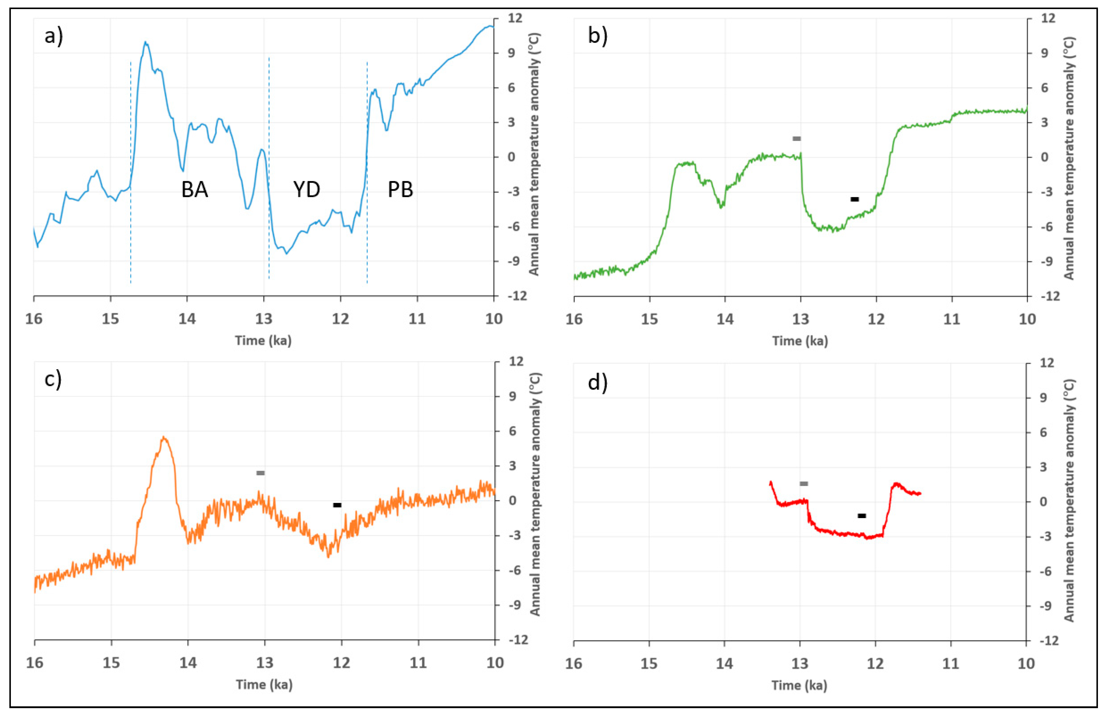
During the last termination, the Younger Dryas cold event (YD) interrupted the overall warming trend with the strongest response in the circum-North Atlantic region [1,2,3]. The YD started around ~12.9 ka with an abrupt termination of the Bølling-Allerød interstadial (BA) and lasted until ~11.7 ka, when a sharp warming signalled the start of the Preboreal (PB, Figure 1a). The abrupt climate changes associated with the YD have been the subject of many studies, based on both proxy evidence and climate model experiments [3,4]. In this paper, I evaluate the similarities and differences between five key modelling studies.
Over the last few decades, the YD has been the target of many modelling studies, using different model setups and experimental designs [5,6,7,8,9,10,11,12,13,14]. Most early work in the 1980s and 1990s was based on snapshot experiments performed with stand-alone atmospheric general circulation models (AGCMs), such as the GISS (Goddard Institute for Space Studies) model [10] or the ECHAM (European Centre—HAMburg) model [11]. In these snapshot experiments, the sea surface temperatures (SSTs) and sea ice conditions in the North Atlantic Ocean were prescribed, based on assumptions on surface ocean cooling and sea ice expansion. Later studies reported transient simulations with full dynamical coupling of the atmosphere-ocean system in which the ocean circulation was free to interact with the atmosphere [12,13]. These simulations relied heavily on the assumed forcing-history, in particular the freshwater forcing representing the melting of the ice sheets in North America and Europe. Essentially, the freshwater forcing was used in these simulations to tune the models to reproduce a climate evolution that is close to what is known from proxy records [12,13]. Recently, a different approach was used in which the model was constrained with selected proxy-based reconstructions in the North Atlantic realm through data-assimilation (DA [14,15]). In the latter approach, proxy data from the North Atlantic realm were used because the YD signal is most clearly expressed in this area [1,2,3], thus providing a clear constraint for the model.
Each of these three approaches has its merits. ACGM simulations are important to study the magnitude and distribution of the atmospheric response given specific changes in surface conditions (SSTs, sea ice, ice sheets, vegetation) (e.g., [16,17,18,19]). The transient coupled atmosphere-ocean simulations, on the other hand, are able to quantify how fast different climate system components respond to forcings and relative to each other, and how the response anomalies evolve in space (e.g., [20,21,22]). Finally, simulations with DA provide insights into what combination of forcings provides a climate response that is best fitted to proxy-based reconstructions and reveal what atmospheric and oceanic circulation is associated with the corresponding response (e.g., [23,24,25,26]).
However, there are also drawbacks associated with each of these three modelling approaches. First, AGCM simulations do not provide information on temporal changes in climate or on dynamical atmosphere-ocean interactions and imply strong assumptions on surface conditions. For example, AGCM simulations of the YD assume a collapsed Atlantic Meridional Overturning Circulation (AMOC), while there is no evidence for this in palaeoceanographic proxies [9,10]. Likewise, the scenarios applied in transient atmosphere-ocean simulations are not necessarily realistic. For instance, freshwater forcing scenarios may not be consistent with sea level records [12,13]. Similarly, the DA technique relies heavily on the proxy-based reconstructions, but these proxy data contain unresolved biases that are highly uncertain [25,26].
By exploring the similarities and differences in the results from these three approaches, insight is provided into the robust features of the YD and into the characteristics of climate variability during this important period. This is especially relevant for the fourth phase of the palaeoclimate modelling intercomparison project (PMIP4, [27]), with multiple modelling groups performing several climate simulations focusing on the last deglaciation 21 to 9 ka BP, including the BA-to-YD change [28].
In this paper, I therefore compare model results from five studies that cover the three discussed approaches: Rind et al. [10], Renssen and Isarin [29], He [13], Menviel et al. [12] and Renssen et al. [14]. I focus on the seasonal and annual response in temperature and precipitation, and address the following questions:
- -
- What is the range in temperature and precipitation response in the five models?
- -
- What robust features of the YD climate can be distinguished?
- -
- What aspects of the YD climate represent the largest uncertainties?
2. Methods
2.1. Models
In this paper, I discuss results from four different global climate models, being the GISS and ECHAM4 AGCMs, the CCSM3 fully coupled AOGCM and the LOVECLIM model of intermediate complexity. Table 1 summarises the main features.
2.1.1. GISS Model
2.1.2. ECHAM4 Model
2.1.3. CCSM3 Model
The CCSM3 model applied by He [13] is a coupled atmosphere-ocean GCM with dynamical components for the ocean, sea ice, atmosphere, land surface and vegetation [33]. The atmospheric component is CAM3, with 26 levels in the vertical and a ~3.75° × 3.75° lat-lon horizontal resolution. CAM3 is coupled to the POP ocean model, with 25 levels in the vertical and 3.6° longitudinal resolution and variable latitudinal resolution, with the finest grid-spacing near the equator.
2.1.4. LOVECLIM Model
LOVECLIM is a global climate model of intermediate complexity [32], of which two different versions were applied in the studies discussed here: version 1.1 by Menviel et al. [12] and the updated version 1.2 by Renssen et al. [14]. Both of these versions are almost identical, as discussed by Goosse at al. [20], and include dynamically coupled modules for the atmosphere, ocean, sea ice and vegetation. The atmospheric component is ECBilt, a quasi-geostrophic model with 3 layers and T21 resolution (translating to ~5.6° × 5.6° lat-lon). ECBilt includes a land-surface module with a bucket model for soil hydrology. VECODE is the vegetation module on the same grid as ECBilt. The ocean component is CLIO and consists of an ocean general circulation model with 20 layers, coupled to a dynamic-thermodynamic sea ice model, both at 3° × 3° lat-lon resolution.
Figure 1.
Overview of annual temperatures during the last deglaciation (16–10 ka), shown as an anomaly relative to the mean over 13.1 to 13.0 ka. (a) GISP2 ice core in central Greenland [34] provided here for reference, with BA = Bølling-Allerød, YD = Younger Dryas, PB = Preboreal. (b) DGNS experiment performed by Menviel et al. [12], (c) ALL experiment reported by He [13], and (d) COMBINED experiment by Renssen et al. [14]. The temperatures in (b–d) are for the North Atlantic Ocean and Europe in the area between 60° W–30° E, and 40–70° N. Indicated are the timings of the samples for BA (small grey bar) and the YD (small black bar) discussed in this paper.

2.2. Experimental Design
2.2.1. GISS Experiments
Rind et al. [10] performed two equilibrium experiments, both with boundary conditions for 11 ka (orbital parameters, ice sheet configuration and land-sea distribution). The timing of the YD start at 11 ka was derived from the chronostratigraphy of Mangerud et al. [35] that is based on 14C years, placing the YD between 11 and 10 14C kyrs BP. The first experiment (11 kW) included modern sea surface conditions and represents the climate during the BA interstadial. In a second experiment (11 kC) representing the YD, cold surface conditions were prescribed in the North Atlantic North of 25° N following the CLIMAP [36] reconstruction for the last glacial maximum (LGM). Both experiments were run for 5 years, but only the output of the last 3 years was used for the analysis.
2.2.2. ECHAM4 Experiments
Results of two equilibrium experiments are discussed here (expGI1e and expGS1), with boundary conditions appropriate for the BA and the YD [29]. These boundary conditions include SSTs and sea ice cover, orbital forcing, ice sheet configuration, greenhouse gas concentrations, vegetation and land-sea distribution. Regarding the prescribed sea surface conditions, cooling and winter sea-ice cover were applied in the Nordic Seas in the BA simulation. In the YD experiment, strong North Atlantic cooling was prescribed [37], in summer based on foraminiferal evidence [38] and in winter on a modelled shutdown of the AMOC [39]. These two experiments were run for 12 years each, of which the last 10 years were used to account for a spin-up of the model.
2.2.3. CCSM3 Experiment
The results of He [13] discussed in this paper are from his ALL transient CCSM3 simulation, performed within the TraCE-21 ka project. The ALL simulation was started in the LGM and was run forward in time until 1990 CE, using transient forcings, including updates of ice sheets for every 500 years. Freshwater was added to the surface ocean at several locations around the North Atlantic and in the Ross and Weddell Seas. This applied freshwater forcing led to an AMOC collapse during the YD around 12 ka. From the transient results (Figure 1c), I selected two 100-year time periods representing the BA (13.1–13.0 ka) and the YD (12.1–12.0 ka).
2.2.4. LOVECLIM Experiments
The setup of the DGNS experiment by Menviel et al. [12] is similar to the ALL simulation reported by He [11], also starting in the LGM and using transient forcings. Also in this experiment, freshwater forcing was applied to the North Atlantic and the Southern Ocean, leading to an AMOC collapse in the YD, this time between 12.8 and 12.4 ka. Similar to the CCSM3 experiment, I selected two 100-year periods (Figure 1b) to cover the BA (13.1–13.0 ka) and the YD (12.3–12.2 ka).
The COMBINED experiment of Renssen et al. [14] started with an equilibrium experiment for the BA, using appropriate forcings for 13 ka, including ice sheets, orbital parameters, greenhouse gas levels and freshwater forcing. This BA climate was used as a starting point for a transient simulation of the YD climate (Figure 1d), with a combination of forcings applied. The YD simulation was constrained through data-assimilation by proxy-based summer temperatures for Europe and selected annual mean SSTs, primarily from the North Atlantic region [14,40]. The YD results discussed here are averages of 96 ensemble members. Further details on the data-assimilation technique can be found in Dubinkina et al. [41]. The forcings consisted of a 3-year freshwater pulse of 5 Sv (1 Sv = 1 × 10⁶ m3 s−1) at the MacKenzie river outlet, a continuous meltwater forcing 0.1 Sv representing the background melt of the Fennoscandian and Laurentide icesheets, and a –0.52 Wm−2 negative radiative forcing, representing the reduction in atmospheric methane and nitrous oxide, and enhanced mineral dust levels. The applied data assimilation forced the model to an anomalous atmospheric circulation state with more frequent northerly atmospheric flow over Northern Europe. The freshwater forcing resulted in AMOC weakening by 50% relative to the BA, but not a shutdown. The recovery to the PB was obtained by turning off the data assimilation and by removing the background melt forcing. From this experiment, also two 100-yr periods were selected for the BA and the YD (Figure 1d).
To enable efficient analysis of all of these model results that were produced at various spatial resolutions, I converted all results to a common 1° latitude by 1° longitude grid, using the bilinear interpolation tool provided by Schulzweida [42]. Using these re-gridded results, I computed ensemble means, and, in addition, I calculated areal means for the change in temperature and precipitation from the BA to the YD. I focus on the following 15 areas: Greenland (70–80° N, 55–25° W), Nordic Seas (70–80° N, 20° W–20° E), Alaska (60–70° N, 165–135° W), Siberia (50–70° N, 70–135° E), Europe (35–70° N, 10°W–40° E), Central North America (35–70° N, 125–70° W), North Atlantic (35–60° N, 55–10° W), East Asia (20–40° N, 85–120° E), North Africa (10–30° N, 15°W–35° E), South America (25° S–0, 70–140° W), South Atlantic (35–5° S, 35°W–10° E), Southern Africa (35–20° S, 15–30° E), Australia (35–15° S, 115–150° E), Southern Ocean (65–55° S, 0–360° W) and Antarctica (90–65° S, 0–360° W). I also compare the model results with the proxy-based reconstructions of YD-BA climate change previously published by Shakun and Carlson [4].
3. Results and Discussion
3.1. Temperature
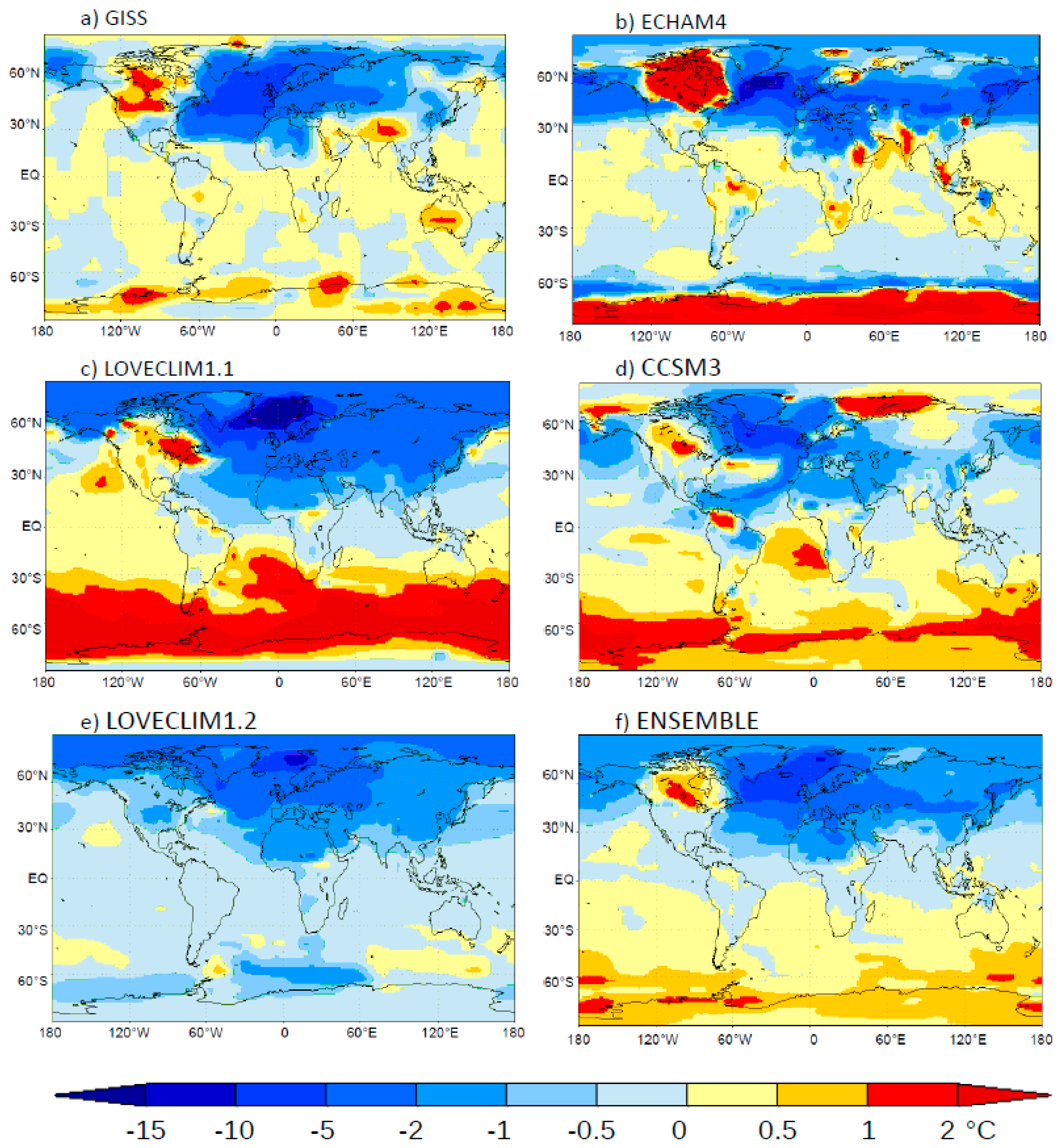
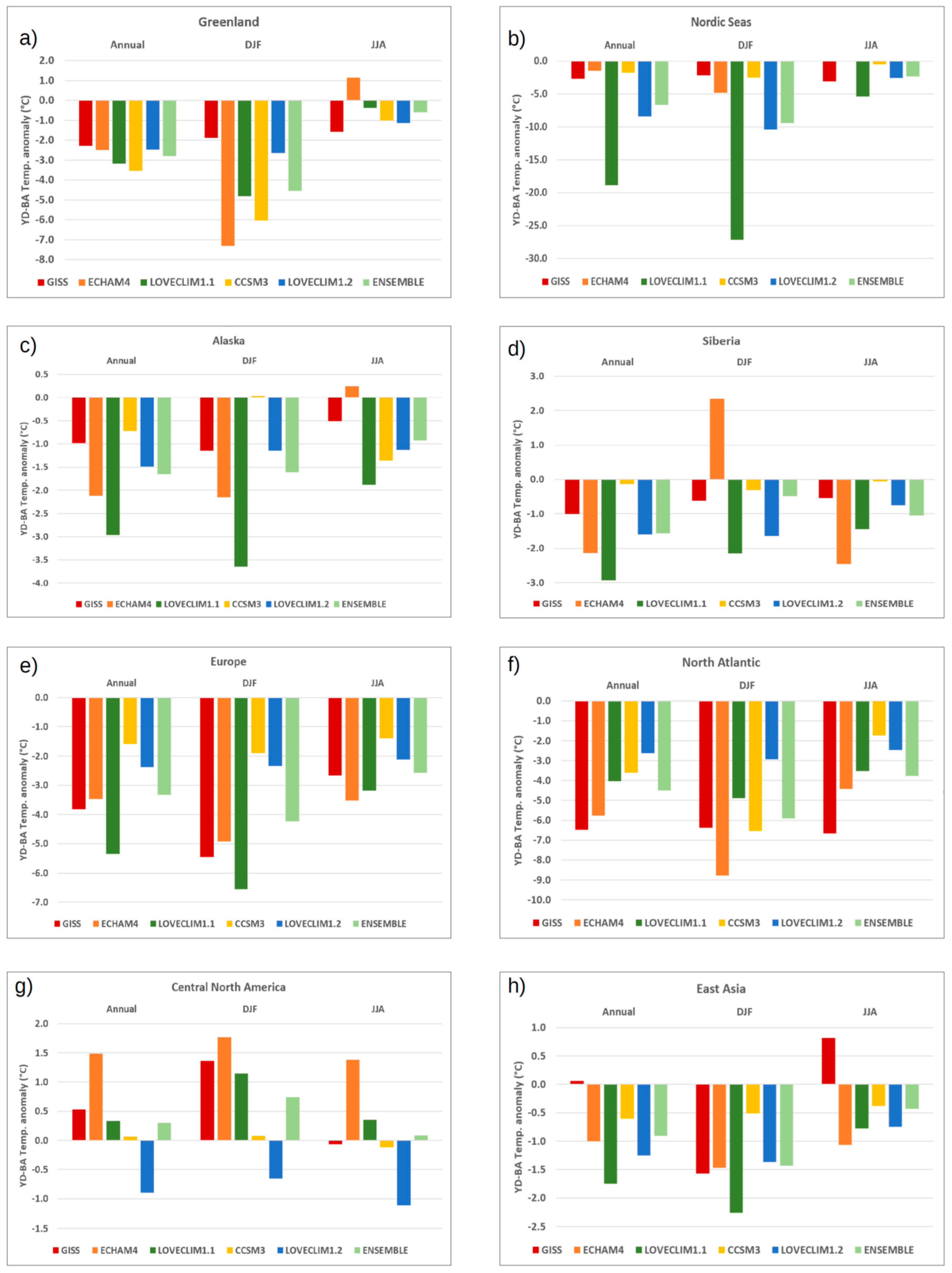
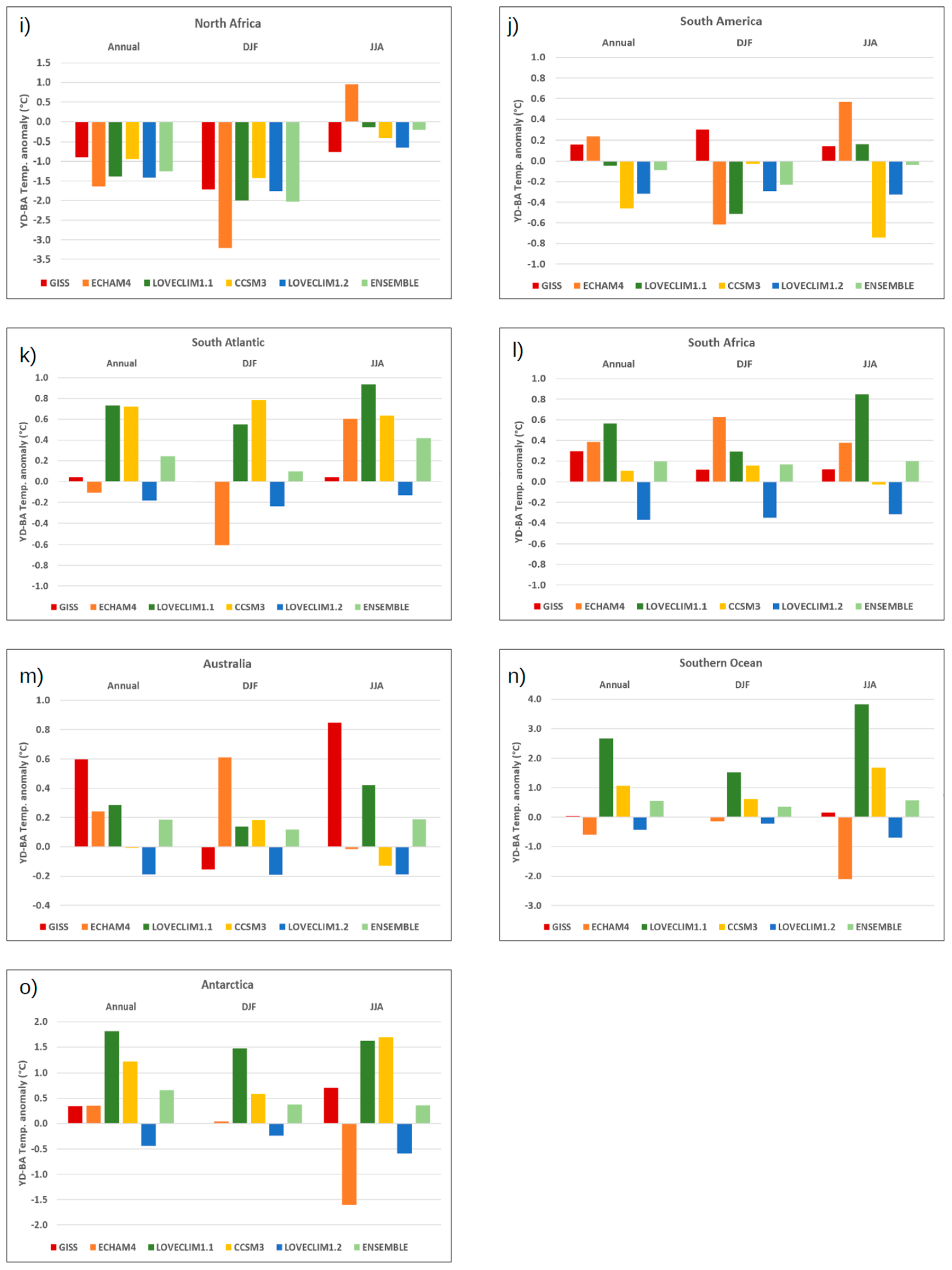
All models consistently simulate an annual mean YD-BA cooling in Europe and over the Nordic Seas and the North Atlantic Ocean (Figure 2 and Figure 3). For these three areas, the models are also consistent in simulating a stronger temperature decline in boreal winter (December-January-February, DJF) than in boreal summer (June-July-August, JJA). Over Europe and the North Atlantic, the magnitude of this cooling is fairly coherent among the models, ranging from −2 to −6 °C for the annual mean YD-BA anomaly (Figure 3). However, the values for the Nordic Seas show also the largest spread of all areas (Figure 3b and Figure 4), where the LOVECLIM1.1 simulation suggests −19 °C for the annual mean, compared to around −2 °C for CCSM3 and ECHAM4. An analysis of Figure 2 suggests that this large deviation between models is related to differences in the implied latitude of North Atlantic Deep Water (NADW) formation. All simulations include strong YD-BA surface cooling over the mid-latitude North Atlantic Ocean, but the latitude of the strongest cooling depends on where the NADW formation takes place before the AMOC perturbation, and this latitude varies considerably among the models. For instance, CCSM3 has the main site of NADW formation between 50 and 60° N, as reflected by the marked cooling (between −5 and −10 °C) between these latitudes in Figure 2d. In this CCSM3 result, however, the cooling in the Nordic Seas is much less (less than −5 °C), in contrast to the result of the two LOVECLIM simulations that have the main NADW formation site and strongest cooling (−10 to −25 °C) more northerly between 70 and 75° N in the Nordic Seas (Figure 2c,e).
In Greenland, Alaska, Siberia, East Asia, and North Africa, four out of five models indicate YD-BA cooling for all the three timeframes. The deviating model is in most cases ECHAM4, with a warming signal during JJA. In Central North America, four models suggest warmer conditions in DJF during the YD relative to the BA, but LOVECLIM1.2 suggests colder YD conditions (−1 °C).
In the remaining regions, all in the Southern Hemisphere (SH), the responses are also diverging (Figure 2 and Figure 3), depending more strongly on the experimental setup. In the two transient modelling studies that assumed a full AMOC collapse (CCSM3 and LOVECLIM1.1), positive YD-BA anomalies were simulated in most SH regions (+2 to +3 °C), most clearly in Antarctica, the Southern Ocean and the South Atlantic (Figure 2c,d and Figure 3k,o). Together with the marked cooling in the North Atlantic, this SH warming clearly reflects the bi-polar seesaw mechanism being active in these models [43,44,45]. When the AMOC is fully active, it transports important amounts of heat from the South Atlantic, over the equator to the North Atlantic Ocean [46], but when the AMOC collapses, this heat is accumulating in the SH, producing anomalous warming [47]. In contrast, the LOVECLIM1.2 study suggests on average negative YD-BA temperature anomalies in most areas of the Southern Hemisphere (Figure 2e). These relatively cool YD conditions reflect the impact of the negative radiative forcing (−0.52 Wm−2, [14]), which in most SH areas overwhelms the warming impact of the relatively weak bi-polar seesaw in the LOVECLIM1.2 study [15].
3.2. Precipitation
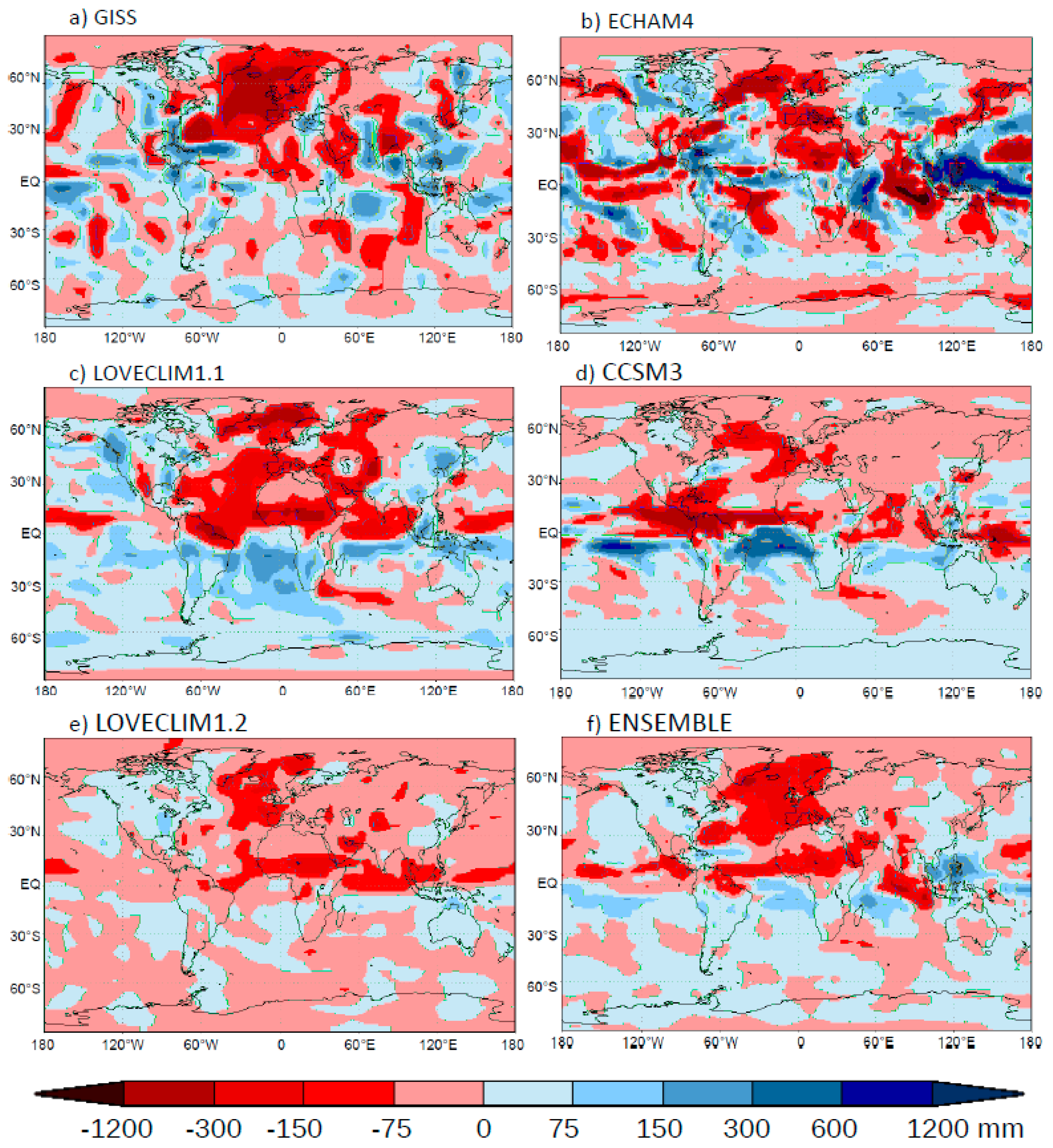
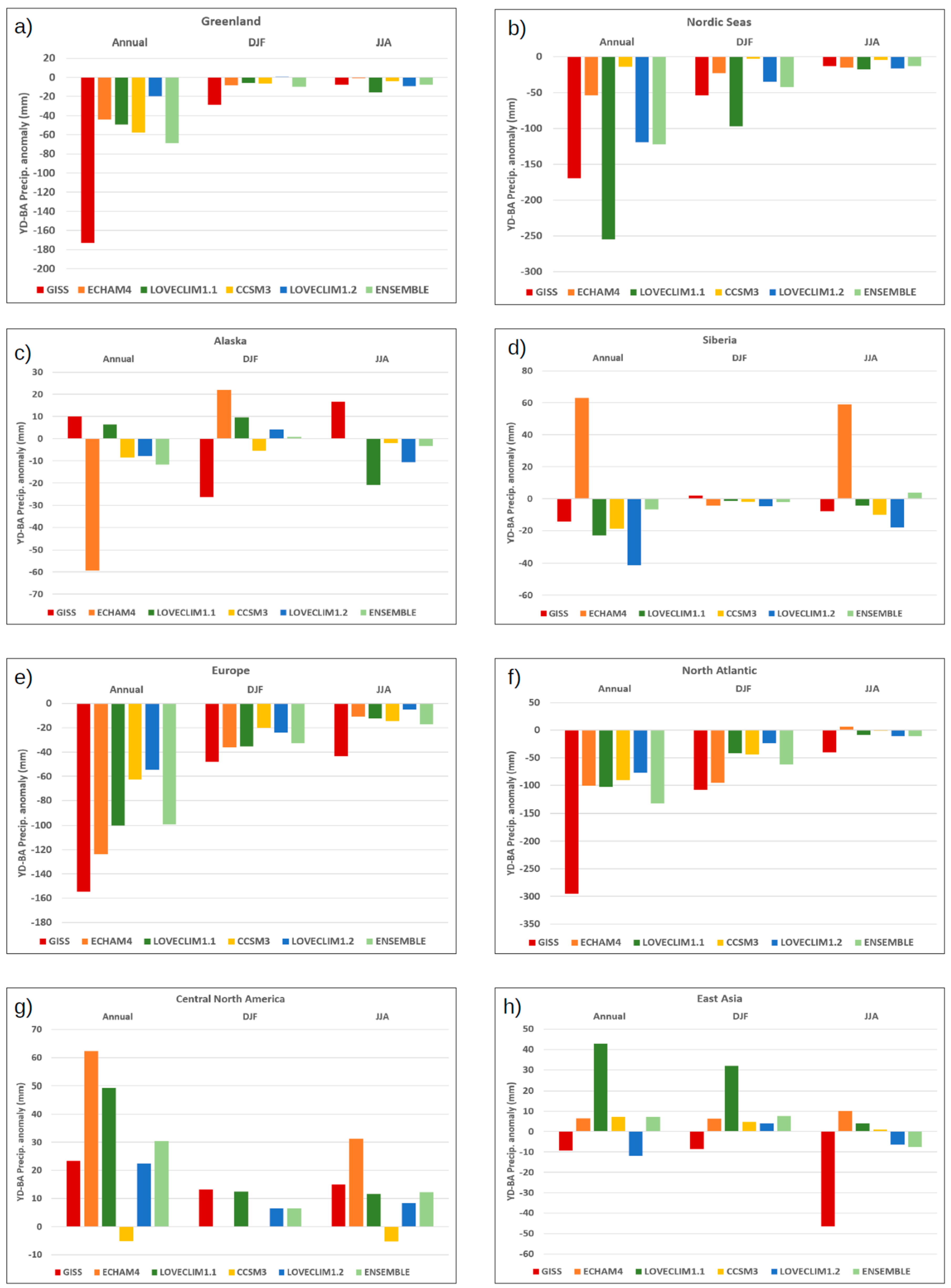
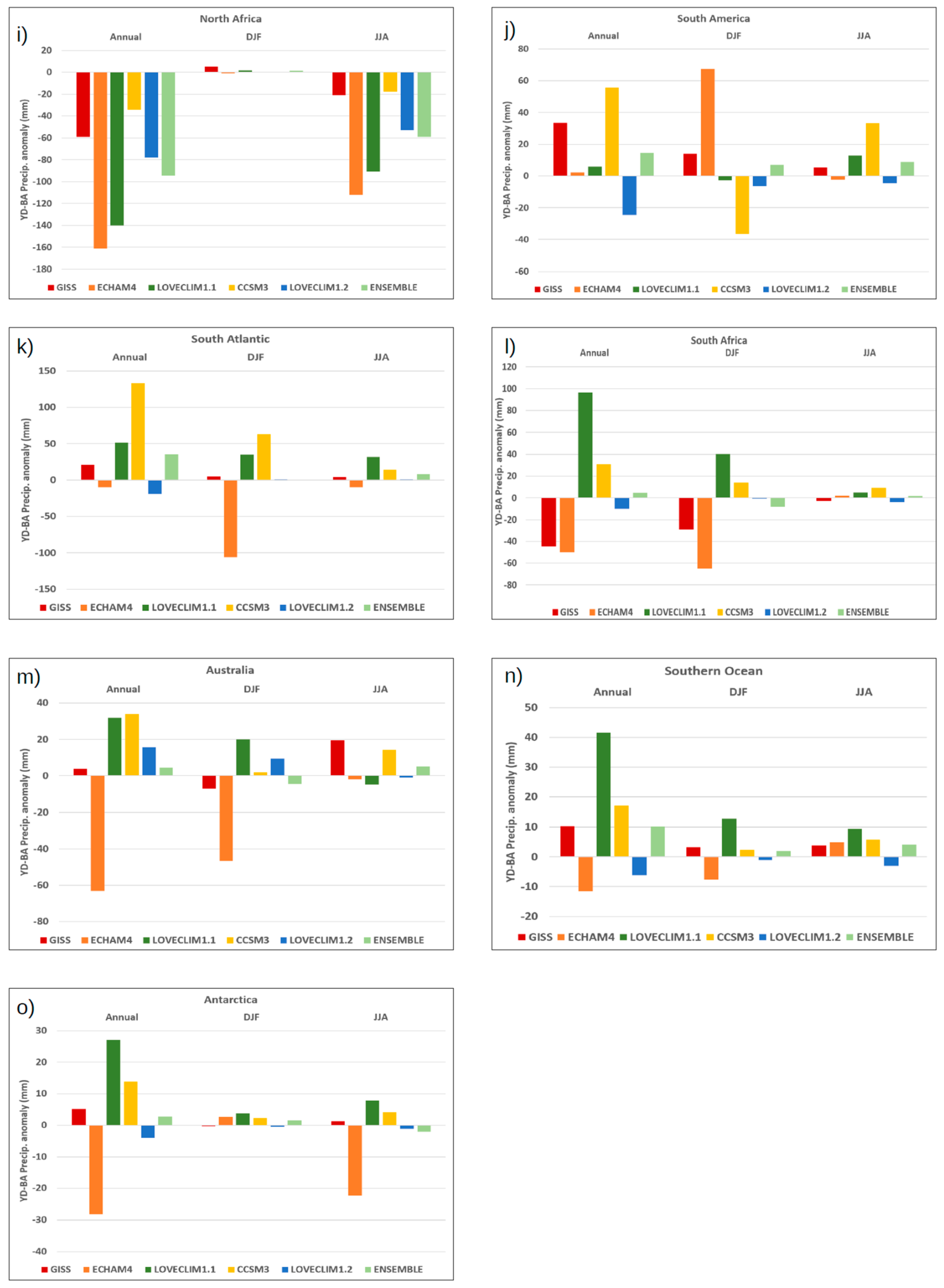
The simulations indicate that most regions with YD-BA cooling experienced also a distinct decrease in precipitation (by as much as 100 mm yr−1), including Europe, North Atlantic, Nordic Seas, Greenland and North Africa (Figure 5 and Figure 6). In areas further away from coldest region (i.e., the North Atlantic Ocean), such as Alaska, Siberia and East Asia, the precipitation response was more subdued and less consistent among the different models (Figure 6c,d,h). In Central North America, 4 out of 5 models simulate a modest increase in precipitation in the YD relative to the BA (+30 mm yr−1 ensemble mean, Figure 6g), in line with the warmer conditions suggested by most models. In the SH, ECHAM4 simulates negative YD-BA anomalies over most areas (Figure 6l–o), which is consistent with relatively cold YD conditions (Figure 2b). In contrast, the models with an active bi-polar seesaw (i.e., CCSM3 and LOVECLIM1.1) simulate mostly positive YD-BA anomalies in the SH (Figure 6j–o), in agreement with increased temperatures (Figure 2c,d).
The response in the tropics is generally similar to the pattern discussed by Renssen et al. [15], with negative and positive YD-BA precipitation anomalies north and south of the equator, respectively. This pattern is clearest in the simulations with full atmosphere-ocean coupling (LOVECLIM1.1/1.2 and CCSM3, Figure 5c,d) and is related to a southward shift of the intertropical convergence zone (ITCZ). This effect is well-known from other simulation studies with a perturbed AMOC, showing that the response enhances with a strong bi-polar seesaw effect (e.g., [13,46]). The two AGCM simulations (GISS and ECHAM, Figure 5a,b), with the surface forcing restricted to the North Atlantic region, do not show this contrasting North-South response in the equatorial region.
3.3. Comparison with Proxy-Based Evidence
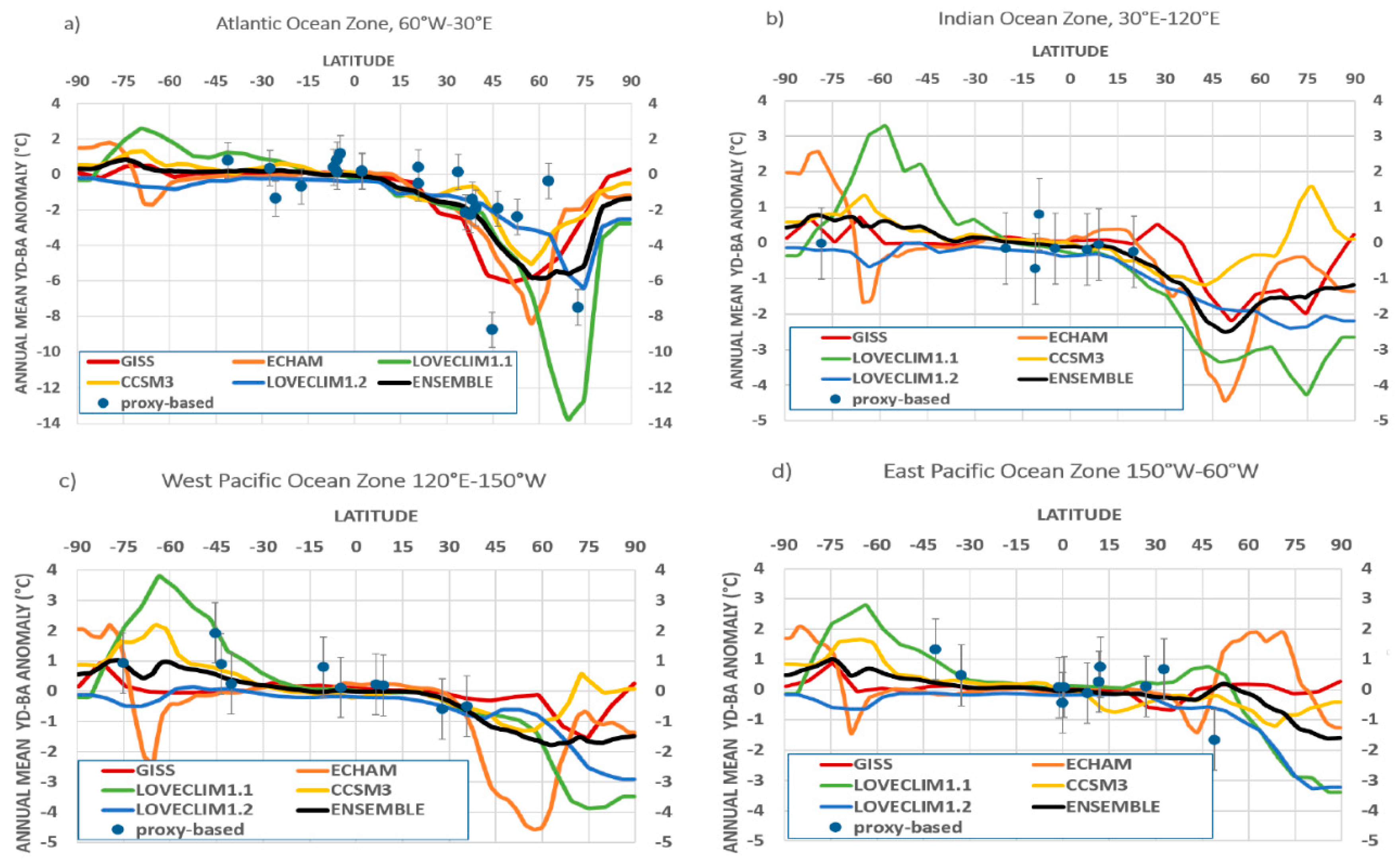
I compare here the modelled temperatures with the global dataset of Shakun and Carlson [4], who provide proxy-based estimates of the annual mean temperature anomaly between the YD and BA. They used a range of proxies, primarily foraminifera-based Mg/Ca ratios and Uk37, and δ18 O on ice cores, foraminifera and speleothems. Shakun and Carlson [4] estimate that the global mean annual temperature was 0.6 °C lower in the YD relative to the BA. Two of the considered models (LOVECLIM1.2 and ECHAM4) simulate an equivalent global mean cooling of −0.6 °C cooling. In the other models in this study, the YD-BA global cooling was less than −0.6 °C, with −0.4 °C for GISS, −0.3 °C for LOVECLIM1.1 and −0.2 °C for CCSM3. The latter two results reflect the impact of a relatively intense SH warming associated with a strong bi-polar seesaw mechanism (compare Figure 2c,d with Figure 2a,b,e). On a global level, these relatively warm conditions in the SH compensate for a considerable part of the cooling in the circum-North Atlantic region. For a more detailed comparison to the individual proxy-based estimates of Shakun and Carlson [4], I divide the data into four zones of 90 degrees of longitude each and compare the proxy-based values with the model-based zonal means (Figure 7).
In the Atlantic Ocean zone (Figure 7a), the models are relatively consistent with a marked YD-BA cooling (−6 to −8 °C) between 45 and 75° N that is in reasonable agreement with the proxy based estimates. An exception is the cooling simulated by LOVECLIM1.1 that appears about twice as strong as the rest of the data. In LOVECLIM1.1, this strong cooling results from a complete shutdown of the AMOC and subsequent cover by sea ice in the Nordic Seas [12]. Again, proxy-based reconstructions of the strength of the ocean circulation suggest that such an AMOC shutdown is unlikely during the YD [48,49,50,51].
The other zones show a divergence of the models at the SH mid-to-high latitudes (Figure 7b–d), suggesting a higher uncertainty here. LOVECLIM1.1 and CCSM3 show clearly warm YD conditions at SH high latitudes while the signal is less clear in the other models. The few available proxy-based estimates of YD-BA temperature change seem to support this warm SH anomaly, at least between 40 and 45° S [52,53,54,55,56]. Unfortunately, the dataset of Shakun and Carlson [4] does not provide estimates from the Southern Ocean around 60° S where the maximum YD warming is simulated. However, to the south of this modelled warming peak, Antarctic ice core records give clear evidence for warmer conditions during the YD time relative to the BA [57].
A major uncertainty is the YD signal over the Arctic Ocean (Figure 7). The simulations performed with LOVECLIM suggest cooler annual mean temperatures here (by 2 to 5 °C, Figure 2c,e and Figure 7a–d), but the other models do not indicate any major cooling of more than 2 °C, and the CCSM3 result even shows warmer conditions over most of the Arctic (Figure 2d). Except for the Greenland ice cores that show marked cooling, the dataset of Shakun and Carlson [4] does unfortunately not include reconstructions of YD-BA temperature change for the Arctic. Other proxy-based evidence from lake and peat records from Eastern Siberia, Southern Alaska suggest distinct YD cooling [58] in agreement with the model results (Figure 2). However, the YD warming reconstructed in Central Alaska, most of Northeastern Siberia and possibly Northern Alaska [58] is not reproduced by the models. Relatively dry YD conditions in Svalbard, as based on the extent of cirque glaciers [59], matches the simulated negative YD-BA precipitation anomaly in the Nordic Seas region (Figure 5).
Concerning the seasonality of the YD-BA signal, all simulations suggest that cooling around the North Atlantic is stronger in boreal winter than in boreal summer (Figure 3a–f) in agreement with proxy data [60,61]. In Europe, the modelled YD-BA summer temperature anomalies (Figure 2 and Figure 3e) agree well with 2 to 3 °C YD-BA cooling in summer as suggested by Renssen and Isarin [29] based on palaeobotanical proxies, and by Heiri et al. [40] based on chironomids. However, the models do not reproduce the proxy-based winter YD-BA cooling of at least 10 °C suggested by Renssen and Isarin [29], although the LOVECLIM1.1 result comes close (Figure 2 and Figure 3e).
The modelling results discussed here give no indication for relative mild YD summer conditions in Europe recently suggested by Schenk et al. [9] based on both model simulations and palaeobotanical proxies. They applied a high-resolution (0.9° × 1.25° lat-lon) version of the CESM1 model that included coupled modules for the atmosphere-land-sea ice system to perform equilibrium simulations of the BA and the YD, using prescribed surface ocean conditions from the transient CCSM3 simulations [13] discussed in this paper. Schenk et al. [9] simulated similar summer temperatures in the YD and the BA in NW and SW Europe and even warmer YD summer conditions in Eastern Europe. Schenk et al. [9] find support for these relatively warm YD summers in reconstructions based on palaeobotanical proxies, using the climate indicator species method. The reconstructed warm summer conditions are based on an alternative interpretation of these palaeobotanical proxies relative to earlier work [29,62]. Further research on proxies for summer temperatures is therefore required to shed light on the nature of the summer YD climate in Europe.
The modelled large-scale patterns of precipitation change agree largely with the proxy-based evidence for hydroclimatic YD-BA change reviewed recently by Renssen et al. [15]. Over continents directly downwind from the cold North Atlantic Ocean, most notably in Europe and North Africa, the models simulate a much drier climate consistent with proxy-based reconstructions (e.g., [63,64,65,66,67,68,69]). However, proxies also indicate drying in East Asia (e.g., [70,71,72,73]), which is not clearly reproduced by the simulations (e.g., Figure 5f). In central North America, 4 out of 5 models suggest an increase in annual precipitation (Figure 6g) that is in agreement with different types of proxy evidence [74,75,76,77]. This enhanced precipitation is caused by an anomalous southerly atmospheric flow, bringing moist air from the Gulf of Mexico northwards to the American continental interior [15].
In the tropics, the models indicate a decrease in precipitation north of the equator and an increase to the south. This is a well-known model response to a weakening of the AMOC and the associated Northern Hemisphere cooling, causing the ITCZ to shift southwards [47]. Proxies from the tropics support this mechanism, showing for instance a wetter climate in Indonesia [78,79], but drying in the Philippines [79]. This North-South contrast in the hydroclimatic response is also found in proxy evidence from South America (e.g., [80]) and Southern Africa (e.g., [81,82]). In contrast to the precipitation, a major equatorial YD temperature signal is absent in both the models and the proxy data.
The proxy-model comparison of the result for LOVECLIM1.1 illustrates the uncertainties surrounding the forcing of the YD climate. On the one hand, the AMOC shutdown in this simulation produces a winter YD-BA cooling in Europe that is matching best with proxies, and a bi-polar seesaw that is consistent with proxy-based evidence for warming in the Southern Ocean and Antarctica. On the other hand, the imposed AMOC shutdown disagrees with palaeoceanographic evidence, and the associated relatively small global YD-BA cooling of −0.3 °C is a clear underestimation of the proxy-based value of −0.6 °C. This mismatch could indicate that the applied YD forcing is not realistic. A possible solution is the alternative YD forcing suggested by Renssen et al. [14], consisting of a weakened AMOC (~50%) with continued overturning in the Atlantic Ocean, producing a weak bi-polar seesaw with some warming at SH mid-to-high latitudes. This oceanic forcing would be combined with a sustained, marked negative radiative forcing related to lowered atmospheric levels of methane and nitrous oxide during the YD and an increased atmospheric dust load, for which ample evidence has been found in ice cores [34,83,84,85]. In the LOVECLIM1.2 simulation, this negative radiative forcing results in YD cooling in many regions in the SH mid-to-high latitudes (Figure 2e), which is supported by some palaeoceanographic evidence [86]. However, the LOVECLIM1.2 result that includes this combined forcing does not produce a satisfactory match with proxy-based evidence everywhere either, as especially the European winter temperatures were underestimated.
The ability of models to reproduce proxy-based climate anomalies is also related to model-specific sensitivity to forcings, making it important to further investigate forcing scenarios with a suite of models as is planned within PMIP4 [28]. In this paper, I compared models of different set-up and complexity, and also the experimental designs were very different. In a future model-intercomparison it is important to apply a more standardised experimental design, and also to involve high-resolution models that include full atmosphere-ocean coupling to explore the inferences of Schenk et al. [9] for mild YD summers in Europe.
4. Conclusions
The comparison of model simulations shows consistent annual YD-BA cooling in Europe, the North Atlantic Ocean, Nordic Seas, Greenland, Alaska and North Africa. In all cases, the area of maximum YD-BA cooling is over the North Atlantic Ocean or the Nordic Seas, ranging from −25 °C to −6 °C. Except for North Africa, the temperature response in the tropics is minor in all simulations. Most models indicate YD-BA warming of up to 2 °C in the interior of North America. Over the Arctic Ocean and the mid-and high latitudes of the Southern Hemisphere, the models show limited agreement. A positive YD-BA anomaly of up to 4 °C was simulated over the Southern Ocean and Antarctica in the two coupled atmosphere-ocean experiments with an AMOC shutdown and a strong bi-polar seesaw effect.
The modelled YD-BA temperature change is generally in agreement with proxy-based evidence for maximum cooling in the circum-North Atlantic region and a strongest temperature response in the winter season. In the simulations discussed here, no indication is found for mild YD summer conditions in Europe, as recently suggested by Schenk et al. [9].
The simulated YD-BA precipitation change is clearly linked to the temperature response. In general, the climate became drier where it was colder, and wetter where it was warmer. The areas with a strongest YD-BA precipitation reduction (by up to 150 mm yr−1) are the North Atlantic Ocean, the Nordic Seas, Western Europe and the northern equatorial region. Over the southern equatorial region, a marked increase in YD-BA precipitation is evident, especially over the oceans. This general precipitation pattern is supported by proxy data.
The coupled atmosphere-ocean simulations with AMOC shutdown agree best with several aspects of proxy-based YD-BA climate response, such as the magnitude of winter cooling in Europe and the warming in the high-latitude Southern Hemisphere. However, the assumed full AMOC collapse is not supported by proxy data and these simulations strongly underestimate the magnitude of global YD-BA global cooling indicated by proxies. This mismatch indicates uncertainty in the YD forcing. It is proposed that negative radiative forcing could have been more important during the YD-BA climate change than assumed until now. This negative radiative forcing would represent higher atmospheric dust levels and reduced concentrations of methane and nitrous oxide during the YD, as evidenced by ice cores.
Funding
This research received no external funding.
Acknowledgments
The author would like to thank the involved modelling groups for making their results available for further analysis, in particular David Rind and the NASA-Godard Institute for Space Studies, Laurie Menviel and The School of Ocean and Earth Science and Technology at the University of Hawaii, and Feng He and the Center of Climatic Research at the University of Wisconsin-Madison.
Conflicts of Interest
The author declares no conflict of interest.
References
- Peteet, D.M. Global Younger Dryas? Quat. Int. 1995, 28, 93–104. [Google Scholar] [CrossRef]
- Clark, P.U.; Shakun, J.D.; Baker, P.A.; Bartlein, P.J.; Brewer, S.; Brook, E.; Carlson, A.E.; Cheng, H.; Kaufman, D.S.; Liu, Z.; et al. Global climate evolution during the last deglaciation. Proc. Natl. Acad. Sci. USA 2012, 109, E1134–E1142. [Google Scholar] [CrossRef] [Green Version]
- Carlson, A.E. The Younger Dryas climate event. In The Encyclopedia of Quaternary Science; Elias, S.A., Ed.; Elsevier: Amsterdam, The Netherlands, 2013; Volume 3, pp. 126–134. [Google Scholar]
- Shakun, J.D.; Carlson, A.E. A global perspective on Last Glacial Maximum to Holocene climate change. Quat. Sci. Rev. 2010, 29, 1801–1816. [Google Scholar] [CrossRef]
- Harvey, L.D. Modelling the younger dryas. Quat. Sci. Rev. 1989, 8, 137–149. [Google Scholar] [CrossRef]
- Mikolajewicz, U.; Crowley, T.J.; Schiller, A.; Voss, R. Modelling teleconnections between the North Atlantic and North Pacific during the Younger Dryas. Nature 1997, 387, 384–387. [Google Scholar] [CrossRef]
- Manabe, S.; Stouffer, R.J. Coupled ocean-atmosphere model response to freshwater input: Comparison to Younger Dryas Event. Paleoceanography 1997, 12, 321–336. [Google Scholar] [CrossRef]
- Peteet, D.M. Late glacial climate variability and General Circulation Model (GCM) experiments: An overview. In Interhemispheric Climate Linkages; Markgraf, V., Ed.; Academic Press: Cambridge, MA, USA, 2001; pp. 417–432. [Google Scholar]
- Schenk, F.; Väliranta, M.; Muschitiello, F.; Tarasov, L.; Heikkilä, M.; Björck, S.; Brandefelt, J.; Johansson, A.V.; Näslund, J.-O.; Wohlfarth, B. Warm summers during the Younger Dryas cold reversal. Nat. Commun. 2018, 9, 1634. [Google Scholar] [CrossRef] [Green Version]
- Rind, D.; Peteet, D.; Broecker, W.; McIntyre, A.; Ruddiman, W. The impact of cold North Atlantic sea surface temperatures on climate: Implications for the Younger Dryas cooling (11–10 k). Clim. Dyn. 1986, 1, 3–33. [Google Scholar] [CrossRef]
- Renssen, H.; Lautenschlager, M.; Schuurmans, C.J.E. The atmospheric winter circulation during the Younger Dryas stadial in the Atlantic/European sector. Clim. Dyn. 1996, 12, 813–824. [Google Scholar] [CrossRef]
- Menviel, L.; Timmermann, A.; Timm, O.E.; Mouchet, A. Deconstructing the Last Glacial termination: The role of millennial and orbital-scale forcings. Quat. Sci. Rev. 2011, 30, 1155–1172. [Google Scholar] [CrossRef]
- He, F. Simulating Transient Climate Evolution of the Last Deglaciation with CCSM3. Ph.D. Thesis, University of Wisconsin-Madison, Madison, WI, USA, 2011; p. 185. [Google Scholar]
- Renssen, H.; Mairesse, A.; Goosse, H.; Mathiot, P.; Heiri, O.; Roche, D.M.; Nisancioglu, K.H.; Valdes, P.J. Multiple causes of the Younger Dryas cold period. Nat. Geosci. 2015, 8, 946–949. [Google Scholar] [CrossRef]
- Renssen, H.; Goosse, H.; Roche, D.M.; Seppä, H. The global hydroclimate response during the Younger Dryas event. Quat. Sci. Rev. 2018, 193, 84–97. [Google Scholar] [CrossRef]
- Members, C. Climatic Changes of the Last 18,000 Years: Observations and Model Simulations. Science 1988, 241, 1043–1052. [Google Scholar] [CrossRef]
- Kutzbach, J.E.; Guetter, P.J.; Behling, P.J.; Selin, R. Simulated climatic changes: Results of the COHMAP climate-model experiments. In Global Climates since the Last Glacial Maximum; Wright, H.E., Jr., Kutzbach, J.E., Webb, T., III, Ruddiman, W.F., Street-Perrott, F.A., Bartlein, P.J., Eds.; University Minnesota Press: Minneapolis, MN, USA, 1993; pp. 24–93. [Google Scholar]
- Kohfeld, K.E.; Harrison, S.P. How well can we simulate past climates? Evaluating the models using global palaenvironmental datasets. Quat. Sci. Rev. 2000, 19, 321–346. [Google Scholar] [CrossRef]
- Braconnot, P.; Otto-Bliesner, B.; Harrison, S.; Joussaume, S.; Peterchmitt, J.-Y.; Abe-Ouchi, A.; Crucifix, M.; Driesschaert, E.; Fichefet, T.; Hewitt, C.D.; et al. Results of PMIP2 coupled simulations of the Mid-Holocene and Last Glacial Maximum—Part 1: Experiments and large-scale features. Clim. Past 2007, 3, 261–277. [Google Scholar] [CrossRef] [Green Version]
- Liu, Z.; Otto-Bliesner, B.L.; He, F.; Brady, E.C.; Tomás, R.; Clark, P.U.; Carlson, A.E.; Lynch-Stieglitz, J.; Curry, W.; Brook, E.; et al. Transient Simulation of Last Deglaciation with a New Mechanism for Bolling-Allerod Warming. Science 2009, 325, 310–314. [Google Scholar] [CrossRef] [Green Version]
- Renssen, H.; Seppä, H.; Heiri, O.; Roche, D.M.; Goosse, H.; Fichefet, T. The spatial and temporal complexity of the Holocene thermal maximum. Nat. Geosci. 2009, 2, 411–414. [Google Scholar] [CrossRef]
- Zhang, Y.; Renssen, H.; Seppä, H.; Valdes, P.J. Holocene temperature trends in the extratropical Northern Hemisphere based on inter-model comparisons. J. Quat. Sci. 2018, 33, 464–476. [Google Scholar] [CrossRef] [Green Version]
- Goosse, H.; Crespin, E.; De Montety, A.; Mann, M.E.; Renssen, H.; Timmermann, A. Reconstructing surface temperature changes over the past 600 years using climate model simulations with data assimilation. J. Geophys. Res. Space Phys. 2010, 115. [Google Scholar] [CrossRef]
- Widmann, M.; Goosse, H.; Van Der Schrier, G.; Schnur, R.; Barkmeijer, J. Using data assimilation to study extratropical Northern Hemisphere climate over the last millennium. Clim. Past 2010, 5, 2115–2156. [Google Scholar] [CrossRef]
- Mairesse, A.; Goosse, H.; Mathiot, P.; Wanner, H.; Dubinkina, S. Investigating the consistency between proxy-based reconstructions and climate models using data assimilation: A mid-Holocene case study. Clim. Past 2013, 9, 2741–2757. [Google Scholar] [CrossRef] [Green Version]
- Mathiot, P.; Goosse, H.; Crosta, X.; Stenni, B.; Braida, M.; Renssen, H.; Van Meerbeeck, C.J.; Masson-Delmotte, V.; Mairesse, A.; Dubinkina, S. Using data assimilation to investigate the causes of Southern Hemisphere high latitude cooling from 10 to 8 ka BP. Clim. Past 2013, 9, 887–901. [Google Scholar] [CrossRef] [Green Version]
- Kageyama, M.; Braconnot, P.; Harrison, S.P.; Haywood, A.M.; Jungclaus, J.H.; Otto-Bliesner, B.L.; Peterschmitt, J.-Y.; Abe-Ouchi, A.; Albani, S.; Bartlein, P.J.; et al. The PMIP4 contribution to CMIP6—Part 1: Overview and over-arching analysis plan. Geosci. Model Dev. 2018, 11, 1033–1057. [Google Scholar] [CrossRef]
- Ivanovic, R.F.; Gregoire, L.G.; Kageyama, M.; Roche, D.M.; Valdes, P.J.; Burke, A.; Drummond, R.; Peltier, W.R.; Tarasov, L. Transient climate simulations of the deglaciation 21–9 thousand years before present (version 1)—PMIP4 Core experiment design and boundary conditions. Geosci. Model Dev. 2016, 9, 2563–2587. [Google Scholar] [CrossRef] [Green Version]
- Renssen, H.; Isarin, R. The two major warming phases of the last deglaciation at ∼14.7 and ∼11.5 ka cal BP in Europe: Climate reconstructions and AGCM experiments. Glob. Planet. Chang. 2001, 30, 117–153. [Google Scholar] [CrossRef]
- Hansen, J.; Russell, G.; Rind, D.; Stone, P.; Lacis, A.; Lebedeff, S.; Ruedy, R.; Travis, L. Efficient Three-Dimensional Global Models for Climate Studies: Models I and II. Mon. Weather Rev. 1983, 3, 609–662. [Google Scholar] [CrossRef]
- Roeckner, E.; Arpe, K.; Bengtsson, L.; Christoph, M.; Claussen, M.; Dümenil, L.; Esch, M.; Giorgetta, M.; Schlese, U.; Schulzweida, U. The atmospheric general circulation model ECHAM-4: Model description and simulation of present-day climate. In Max-Planck-Institute for Meteorology Report 218; Max-Planck_Institute for Meteorology: Hamburg, Germany, 1996; p. 90. [Google Scholar]
- Collins, W.D.; Bitz, C.M.; Blackmon, M.L.; Bonan, G.B.; Bretherton, C.S.; Carton, J.A.; Chang, P.; Doney, S.C.; Hack, J.J.; Henderson, T.B.; et al. The Community Climate System Model Version 3 (CCSM3). J. Clim. 2006, 19, 2122–2143. [Google Scholar] [CrossRef]
- Goosse, H.; Brovkin, V.; Fichefet, T.; Haarsma, R.; Huybrechts, P.; Jongma, J.; Mouchet, A.; Selten, F.; Barriat, P.-Y.; Campin, J.-M.; et al. Description of the Earth system model of intermediate complexity LOVECLIM version 1.2. Geosci. Model Dev. 2010, 3, 603–633. [Google Scholar] [CrossRef] [Green Version]
- Alley, R.B. The Younger Dryas cold interval as viewed from central Greenland. Quat. Sci. Rev. 2000, 19, 213–226. [Google Scholar] [CrossRef]
- Mangerud, J.; Andersen, S.T.; Berglund, B.E.; Donner, J.J. Quaternary stratigraphy of Norden, a proposal for terminology and classification. Boreas 1974, 3, 109–126. [Google Scholar] [CrossRef]
- CLIMAP Project. Seasonal Reconstruction of the Earth’s Surface at the Last Glacial Maximum; Geological Society of America: Boulder, CO, USA, 1981. [Google Scholar]
- Renssen, H. The global response to Younger Dryas boundary conditions in an AGCM simulation. Clim. Dyn. 1997, 13, 587–599. [Google Scholar] [CrossRef]
- Sarnthein, M.; Jansen, E.; Weinelt, M.; Arnold, M.; Duplessy, J.C.; Erlenkeuser, H.; Flatøy, A.; Johannessen, G.; Johannessen, T.; Jung, S.; et al. Variations in Atlantic surface ocean paleoceanography, 50°–80°N: A time-slice record of the last 30 000 years. Paleoceanography 1995, 10, 1063–1094. [Google Scholar] [CrossRef] [Green Version]
- Schiller, A.; Mikolajewicz, U.; Voss, R. The stability of the thermohaline circulation in a coupled ocean-atmosphere circulation model. Clim. Dyn. 1997, 13, 325–347. [Google Scholar] [CrossRef] [Green Version]
- Heiri, O.; Brooks, S.J.; Renssen, H.; Bedford, A.; Hazekamp, M.; Ilyashuk, B.P.; Jeffers, E.S.; Lang, B.; Kirilova, E.; Kuiper, S.; et al. Validation of climate model-inferred regional temperature change for late-glacial Europe. Nat. Commun. 2014, 5, 4914. [Google Scholar] [CrossRef]
- Dubinkina, S.; Goosse, H.; Sallaz-Damaz, Y.; Crespin, E.; Crucifix, M. Testing a particle filter to reconstruct climate changes over the past centuries. Int. J. Bifurc. Chaos 2011, 21, 3611–3618. [Google Scholar] [CrossRef]
- Schulzweida, U. Climate Data Operator—CDO User Guide; Max-Planck-Institute for Meteorology: Hamburg, Germany, 2019; p. 216. [Google Scholar]
- Crowley, T.J. North Atlantic Deep Water cools the southern hemisphere. Paleoceanography 1992, 7, 489–497. [Google Scholar] [CrossRef]
- Broecker, W.S. Paleocean circulation during the Last Deglaciation: A bipolar seesaw? Paleoceanography 1998, 13, 119–121. [Google Scholar] [CrossRef]
- Stocker, T.F. The Seesaw Effect. Science 1998, 282, 61–62. [Google Scholar] [CrossRef]
- Seidov, D.; Maslin, M. Atlantic ocean heat piracy and the bipolar climate see-saw during Heinrich and Dansgaard-Oeschger events. J. Quat. Sci. 2001, 16, 321–328. [Google Scholar] [CrossRef]
- Stouffer, R.J.; Yin, J.; Gregory, J.; Dixon, K.; Spelman, M.J.; Hurlin, W.; Weaver, A.J.; Eby, M.; Flato, G.M.; Hasumi, H.; et al. Investigating the Causes of the Response of the Thermohaline Circulation to Past and Future Climate Changes. J. Clim. 2006, 19, 1365–1387. [Google Scholar] [CrossRef] [Green Version]
- McManus, J.F.; Francois, R.; Gherardi, J.-M.; Keigwin, L.D.; Brown-Leger, S. Collapse and rapid resumption of Atlantic meridional circulation linked to deglacial climate changes. Nature 2004, 428, 834–837. [Google Scholar] [CrossRef] [PubMed]
- Piotrowski, A.M.; Goldstein, S.L.; Hemming, S.R.; Fairbanks, R.G. Intensification and variability of ocean thermohaline circulation through the last deglaciation. Earth Planet. Sci. Lett. 2004, 225, 205–220. [Google Scholar] [CrossRef]
- Stanford, J.D.; Rohling, E.J.; Hunter, S.; Roberts, A.P.; Rasmussen, S.O.; McManus, J.; Fairbanks, R.G.; Bard, E. Timing of meltwater pulse 1a and climate responses to meltwater injections. Paleoceanography 2006, 21, 4103. [Google Scholar] [CrossRef]
- Barker, S.; Knorr, G.; Mleneck-Vautravers, M.J.; Diz, P.; Skinner, L.C. Extreme deepening of the Atlantic overturning circulation during deglaciation. Nat. Geosci. 2010, 3, 567–571. [Google Scholar] [CrossRef]
- Sachs, J.P.; Affolter, M.; Mann, R. Glacial Surface Temperatures of the Southeast Atlantic Ocean. Science 2001, 293, 2077–2079. [Google Scholar] [CrossRef] [Green Version]
- Kaiser, J.; Lamy, F.; Hebbeln, D. A 70-kyr sea surface temperature record off southern Chile (Ocean Drilling Program Site 1233). Paleoceanography 2005, 20. [Google Scholar] [CrossRef] [Green Version]
- Pahnke, K.; Sachs, J.P. Sea surface temperatures of southern midlatitudes 0-160 kyr B.P. Paleoceanography 2006, 21, 21. [Google Scholar] [CrossRef]
- Barrows, T.T.; Lehman, S.J.; Fifield, L.K.; De Deckker, P. Absence of Cooling in New Zealand and the Adjacent Ocean During the Younger Dryas Chronozone. Science 2007, 318, 86–89. [Google Scholar] [CrossRef] [Green Version]
- Lamy, F.; Kaiser, J.; Arz, H.; Hebbeln, D.; Ninnemann, U.; Timm, O.; Timmermann, A.; Toggweiler, J. Modulation of the bipolar seesaw in the Southeast Pacific during Termination 1. Earth Planet. Sci. Lett. 2007, 259, 400–413. [Google Scholar] [CrossRef] [Green Version]
- Stenni, B.; Buiron, D.; Frezzotti, M.; Albani, S.; Barbante, C.; Bard, E.; Barnola, J.M.; Baroni, M.; Baumgartner, M.; Bonazza, M.; et al. Expression of the bipolar see-saw in Antarctic climate records during the last deglaciation. Nat. Geosci. 2010, 4, 46–49. [Google Scholar] [CrossRef]
- Kokorowski, H.; Anderson, P.; Mock, C.; Lozhkin, A. A re-evaluation and spatial analysis of evidence for a Younger Dryas climatic reversal in Beringia. Quat. Sci. Rev. 2008, 27, 1710–1722. [Google Scholar] [CrossRef]
- Mangerud, J.; Landvik, J.Y. Younger Dryas cirque glaciers in western Spitsbergen: Smaller than during the Little Ice Age. Boreas 2007, 36, 278–285. [Google Scholar] [CrossRef]
- Isarin, R.F.B.; Renssen, H.; Vandenberghe, J. The impact of the North Atlantic Ocean on the Younger Dryas climate in northwestern and central Europe. J. Quat. Sci. 1998, 13, 447–453. [Google Scholar] [CrossRef]
- Denton, G.H.; Alley, R.B.; Comer, G.C.; Broecker, W.S. The role of seasonality in abrupt climate change. Quat. Sci. Rev. 2005, 24, 1159–1182. [Google Scholar] [CrossRef]
- Isarin, R.F.; Bohncke, S.J. Mean July Temperatures during the Younger Dryas in Northwestern and Central Europe as Inferred from Climate Indicator Plant Species. Quat. Res. 1999, 51, 158–173. [Google Scholar] [CrossRef]
- Gasse, F. Hydrological changes in the African tropics since the Last Glacial Maximum. Quat. Sci. Rev. 2000, 19, 189–211. [Google Scholar] [CrossRef]
- Genty, D.; Blamart, D.; Ghaleb, B.; Plagnes, V.; Causse, C.; Bakalowicz, M.; Zouari, K.; Chkir, N.; Hellstrom, J.; Wainer, K. Timing and dynamics of the last deglaciation from European and North African δ13C stalagmite profiles—Comparison with Chinese and South Hemisphere stalagmites. Quat. Sci. Rev. 2006, 25, 2118–2142. [Google Scholar] [CrossRef]
- Foerster, V.E.; Junginger, A.; Langkamp, O.; Gebru, T.; Asrat, A.; Umer, M.; Lamb, H.F.; Wennrich, V.; Rethemeyer, J.; Nowaczyk, N.; et al. Climatic change recorded in the sediments of the Chew Bahir basin, southern Ethiopia, during the last 45,000 years. Quat. Int. 2012, 274, 25–37. [Google Scholar] [CrossRef]
- Rach, O.; Brauer, A.; Wilkes, H.; Sachse, D. Delayed hydrological response to Greenland cooling at the onset of the Younger Dryas in western Europe. Nat. Geosci. 2014, 7, 109–112. [Google Scholar] [CrossRef]
- Rach, O.; Kahmen, A.; Brauer, A.; Sachse, D. A dual-biomarker approach for quantification of changes in relative humidity from sedimentary lipid D∕H ratios. Clim. Past 2017, 13, 741–757. [Google Scholar] [CrossRef] [Green Version]
- Muschitiello, F.; Pausata, F.S.R.; Watson, J.E.; Smittenberg, R.; Salih, A.A.M.; Brooks, S.J.; Whitehouse, N.J.; Karlatou-Charalampopoulou, A.; Wohlfarth, B. Fennoscandian freshwater control on Greenland hydroclimate shifts at the onset of the Younger Dryas. Nat. Commun. 2015, 6, 8939. [Google Scholar] [CrossRef] [Green Version]
- Wang, Y.J.; Cheng, H.; Edwards, R.L.; An, Z.S.; Wu, J.Y.; Shen, C.-C.; Dorale, J.A. A High-Resolution Absolute-Dated Late Pleistocene Monsoon Record from Hulu Cave, China. Science 2001, 294, 2345–2348. [Google Scholar] [CrossRef] [PubMed] [Green Version]
- Chen, F.; Xu, Q.; Chen, J.; Birks, H.J.B.; Liu, J.; Zhang, S.; Jin, L.; Kandasamy, S.; Telford, R.J.; Cao, X.; et al. East Asian summer monsoon precipitation variability since the last deglaciation. Sci. Rep. 2015, 5, 11186. [Google Scholar] [CrossRef] [PubMed] [Green Version]
- Wu, J.; Liu, Q.; Wang, L.; Chu, G.-Q.; Liu, J.-Q. Vegetation and Climate Change during the Last Deglaciation in the Great Khingan Mountain, Northeastern China. PLoS ONE 2016, 11, e0146261. [Google Scholar] [CrossRef]
- Goldsmith, Y.; Broecker, W.S.; Xu, H.; Polissar, P.J.; Demenocal, P.B.; Porat, N.; Lan, J.; Cheng, P.; Zhou, W.; An, Z. Northward extent of East Asian monsoon covaries with intensity on orbital and millennial timescales. Proc. Natl. Acad. Sci. USA 2017, 114, 1817–1821. [Google Scholar] [CrossRef] [PubMed] [Green Version]
- Shanahan, T.M.; McKay, N.P.; Hughen, K.A.; Overpeck, J.; Otto-Bliesner, B.; Heil, C.W.; King, J.; Scholz, C.A.; Peck, J. The time-transgressive termination of the African Humid Period. Nat. Geosci. 2015, 8, 140–144. [Google Scholar] [CrossRef]
- Polyak, V.J.; Rasmussen, J.B.; Asmerom, Y. Prolonged wet period in the southwestern United States through the Younger Dryas. Geology 2004, 32, 5. [Google Scholar] [CrossRef]
- Grimm, E.C.; Watts, W.A.; Jr., G.L.J.; Hansen, B.C.; Almquist, H.R.; Dieffenbacher-Krall, A.C. Evidence for warm wet Heinrich events in Florida. Quat. Sci. Rev. 2006, 25, 2197–2211. [Google Scholar] [CrossRef]
- Wagner, J.D.M.; Cole, J.E.; Beck, J.W.; Patchett, P.J.; Henderson, G.M.; Barnett, H.R. Moisture variability in the southwestern United States linked to abrupt glacial climate change. Nat. Geosci. 2010, 3, 110–113. [Google Scholar] [CrossRef]
- Voelker, S.L.; Stambaugh, M.C.; Guyette, R.P.; Feng, X.; Grimley, D.A.; Leavitt, S.W.; Panyushkina, I.; Grimm, E.C.; Marsicek, J.P.; Shuman, B.; et al. Deglacial hydroclimate of mid-continental North America. Quat. Res. 2015, 83, 336–344. [Google Scholar] [CrossRef]
- Griffiths, M.L.; Drysdale, R.; Vonhof, H.B.; Gagan, M.K.; Zhao, J.-X.; Ayliffe, L.K.; Hantoro, W.S.; Hellstrom, J.; Cartwright, I.; Frisia, S.; et al. Younger Dryas–Holocene temperature and rainfall history of southern Indonesia from δ18O in speleothem calcite and fluid inclusions. Earth Planet. Sci. Lett. 2010, 295, 30–36. [Google Scholar] [CrossRef]
- Partin, J.; Quinn, T.; Shen, C.-C.; Okumura, Y.; Cardenas, M.B.; Siringan, F.; Banner, J.; Lin, K.; Hu, H.-M.; Taylor, F. Gradual onset and recovery of the Younger Dryas abrupt climate event in the tropics. Nat. Commun. 2015, 6, 8061. [Google Scholar] [CrossRef] [PubMed]
- Baker, P.A.; Rigsby, C.A.; Seltzer, G.O.; Fritz, S.C.; Lowenstein, T.K.; Bacher, N.P.; Veliz, C. Tropical climate changes at millennial and orbital timescales on the Bolivian Altiplano. Nature 2001, 409, 698–701. [Google Scholar] [CrossRef]
- Shi, N.; Dupont, L.; Beug, H.-J.; Schneider, R. Correlation between Vegetation in Southwestern Africa and Oceanic Upwelling in the Past 21,000 Years. Quat. Res. 2000, 54, 72–80. [Google Scholar] [CrossRef]
- Dupont, L.; Kim, J.-H.; Schneider, R.; Shi, N. Southwest African climate independent of Atlantic sea surface temperatures during the Younger Dryas. Quat. Res. 2004, 61, 318–324. [Google Scholar] [CrossRef]
- Mayewski, P.A.; Meeker, L.D.; Whitlow, S.; Twickler, M.S.; Morrison, M.C.; Alley, R.B.; Bloomfield, P.; Taylor, K. The Atmosphere during the Younger Dryas. Science 1993, 261, 195–197. [Google Scholar] [CrossRef]
- Monnin, E.; Steig, E.J.; Siegenthaler, U.; Kawamura, K.; Schwander, J.; Stauffer, B.; Stocker, T.F.; Morse, D.L.; Barnola, J.-M.; Bellier, B.; et al. Evidence for substantial accumulation rate variability in Antarctica during the Holocene, through synchronization of CO2 in the Taylor Dome, Dome C and DML ice cores. Earth Planet. Sci. Lett. 2004, 224, 45–54. [Google Scholar] [CrossRef] [Green Version]
- Schilt, A.; Baumgartner, M.; Schwander, J.; Buiron, D.; Capron, E.; Chappellaz, J.; Loulergue, L.; Schüpbach, S.; Spahni, R.; Fischer, H.; et al. Atmospheric nitrous oxide during the last 140,000years. Earth Planet. Sci. Lett. 2010, 300, 33–43. [Google Scholar] [CrossRef]
- Andres, M.S.; Bernasconi, S.M.; A McKenzie, J.; Röhl, U. Southern Ocean deglacial record supports global Younger Dryas. Earth Planet. Sci. Lett. 2003, 216, 515–524. [Google Scholar] [CrossRef]
Figure 2.
Simulated YD-BA annual mean temperature anomaly. (a) GISS, (b) ECHAM4, (c) LOVECLIM1.1, (d) CCSM3, (e) LOVECLIM1.2, (f) ensemble mean. Table 1 provides background information on the used models and on the experimental design.
Figure 2.
Simulated YD-BA annual mean temperature anomaly. (a) GISS, (b) ECHAM4, (c) LOVECLIM1.1, (d) CCSM3, (e) LOVECLIM1.2, (f) ensemble mean. Table 1 provides background information on the used models and on the experimental design.

Figure 3.
Areal average YD-BA temperature anomalies for the annual, December-January-February (DJF) and June-July-August (JJA) means for 15 selected areas: (a) Greenland, (b) Nordic Seas, (c) Alaska, (d) Siberia, (e) Europe, (f) North Atlantic, (g) central North America, (h) East Asia, (i) North Africa, (j) South America, (k) South Atlantic, (l) South Africa, (m) Australia, (n) Southern Ocean, (o) Antarctica.


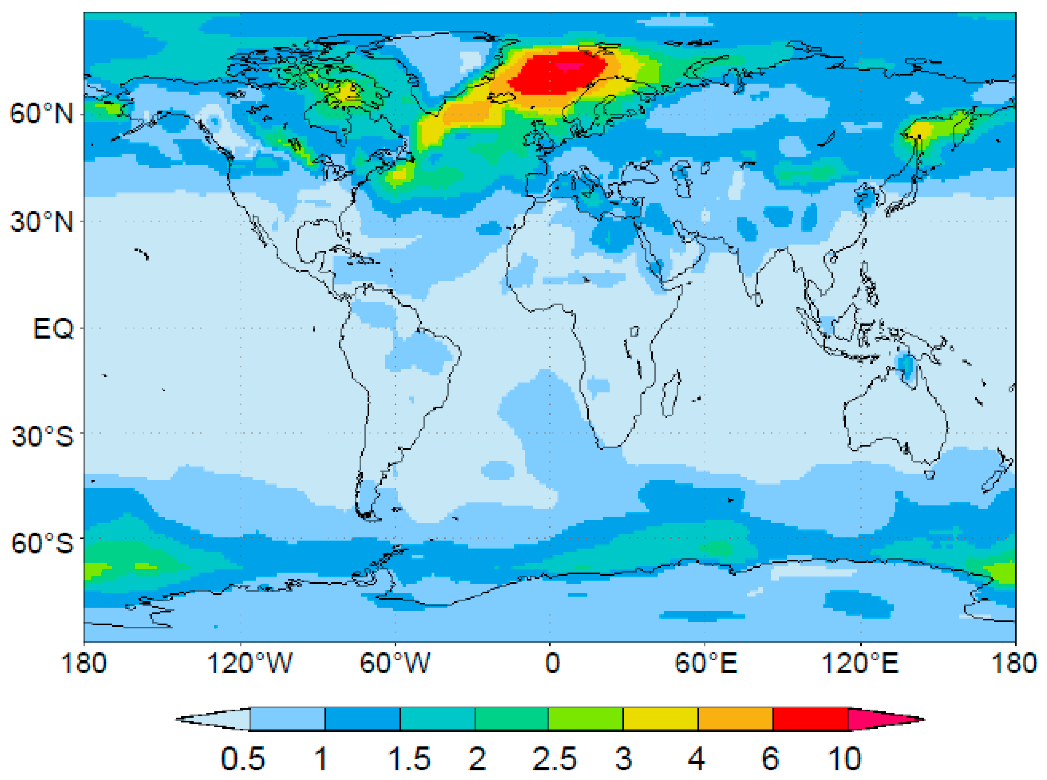
Figure 4.
Standard deviation (°C) for the annual mean YD-BA temperature anomaly, based on the 5 experiments summarised in Table 1.
Figure 4.
Standard deviation (°C) for the annual mean YD-BA temperature anomaly, based on the 5 experiments summarised in Table 1.

Figure 5.
Simulated YD-BA annual mean precipitation anomaly (mm yr−1). (a) GISS, (b) ECHAM4, (c) LOVECLIM1.1, (d) CCSM3, (e) LOVECLIM1.2, (f) ensemble mean.
Figure 5.
Simulated YD-BA annual mean precipitation anomaly (mm yr−1). (a) GISS, (b) ECHAM4, (c) LOVECLIM1.1, (d) CCSM3, (e) LOVECLIM1.2, (f) ensemble mean.

Figure 6.
Areal average YD-BA precipitation anomalies (in mm) for the annual, DJF and JJA means for 15 selected areas: (a) Greenland, (b) Nordic Seas, (c) Alaska, (d) Siberia, (e) Europe, (f) North Atlantic, (g) central North America, (h) East Asia, (i) North Africa, (j) South America, (k) South Atlantic, (l) South Africa, (m) Australia, (n) Southern Ocean, (o) Antarctica.


Figure 7.
Zonal average YD-BA temperature anomalies for 4 zones: (a) Atlantic Ocean zone, (b) Indian Ocean zone, (c) West Pacific Ocean zone, (d) East Pacific Ocean zone. The blue circles show proxy-based estimates published by Shakun and Carlson [4], with bars providing a conservative ±1 °C uncertainty estimate.


Table 1.
Overview of the experiments discussed in this paper.
| Original Reference | Model | Equilibrium or Transient | Model Summary | Experiment Summary |
|---|---|---|---|---|
| Rind et al. [10] | GISS | equilibrium | AGCM, 9 vertical layers, 8° × 10° lat-lon [30] | Last 3 yrs from two 5-yr simulations: 11 kW representing the BA with 11 k boundary conditions and modern SSTs, 11 kC, representing the YD, as 11 kW, but with glacial SSTs in the North Atlantic north of 25° N |
| Renssen & Isarin [29] | ECHAM4 | equilibrium | AGCM, 19 vertical layers, 2.8° × 2.8° lat-lon [31] | Last 10 yrs from two 12-yr simulations: expGI1e, representing the BA, with boundary conditions for Bølling, and expGS1, representing the YD |
| Menviel et al. [12] | LOVECLIM1.1 | transient | EMIC, OGCM 3° × 3° lat-lon, 20 layers, atmospheric quasi-geostrophic model, 3 layers and 5.6° × 5.6° lat-lon, VECODE vegetation model [32] | DGNS: transient simulation 21 to 10 ka with time-varying forcings: insolation, ice sheets (every 100 yr), CO2. Other GHG not changed. Freshwater forcing in both NH and SH |
| He [13] | CCSM3 | transient | Coupled AOVGCM, CAM 3 atmospheric model with 26 layers and ~3.75° × 3.75° lat-lon horizontal resolution. POP ocean model with 25 layers [33] | ALL: transient simulation 22 ka to 1990 CE, time-varying forcings: insolation, ice sheets (every 500 yr), freshwater forcing in both NH and SH |
| Renssen et al. [14] | LOVECLIM1.2 | transient | EMIC, OGCM 3° × 3° lat-lon, 20 layers, atmospheric quasi-geostrophic model, 3 layers and 5.6° × 5.6° lat-lon, VECODE vegetation model [32] | COMBINED: transient simulation starting from 13 ka BA state. Forcings: freshwater forcing in NH, negative radiative forcing, data assimilation (particle filter with 96 ensemble members) |
© 2020 by the author. Licensee MDPI, Basel, Switzerland. This article is an open access article distributed under the terms and conditions of the Creative Commons Attribution (CC BY) license (http://creativecommons.org/licenses/by/4.0/).
Share and Cite
MDPI and ACS Style
Renssen, H. Comparison of Climate Model Simulations of the Younger Dryas Cold Event. Quaternary 2020, 3, 29. https://0-doi-org.brum.beds.ac.uk/10.3390/quat3040029
AMA Style
Renssen H. Comparison of Climate Model Simulations of the Younger Dryas Cold Event. Quaternary. 2020; 3(4):29. https://0-doi-org.brum.beds.ac.uk/10.3390/quat3040029
Chicago/Turabian StyleRenssen, Hans. 2020. "Comparison of Climate Model Simulations of the Younger Dryas Cold Event" Quaternary 3, no. 4: 29. https://0-doi-org.brum.beds.ac.uk/10.3390/quat3040029