The First Two Decades of Neutron Scattering at the Chalk River Laboratories


Northern Stress Technologies, 208, Pine Point Rd., Deep River, ON K0J 1P0, Canada
Quantum Beam Sci. 2021, 5(1), 3; https://0-doi-org.brum.beds.ac.uk/10.3390/qubs5010003
Submission received: 15 December 2020
/
Revised: 8 January 2021
/
Accepted: 11 January 2021
/
Published: 18 January 2021
(This article belongs to the Collection Facilities)
Abstract
:The early advances in neutron scattering at the Chalk River Laboratories of Atomic Energy of Canada are recorded. From initial nuclear physics measurements at the National Research Experimental (NRX) reactor came the realization that, with the flux available and improvements in monochromator technology, direct measurements of the normal modes of vibrations of solids and the structure and dynamics of liquids would be feasible. With further flux increases at the National Research Universal (NRU) reactor, the development of the triple-axis crystal spectrometer, and the invention of the constant-Q technique, the fields of lattice dynamics and magnetism and their interpretation in terms of the long-range forces between atoms and exchange interactions between spins took a major step forward. Experiments were performed over a seven-year period on simple metals such as potassium, complex metals such as lead, transition metals, semiconductors, and alkali halides. These were analyzed in terms of the atomic forces and demonstrated the long-range nature of the forces. The first measurements of spin wave excitations, in magnetite and in the 3D metal alloy CoFe, also came in this period. The first numerical estimates of the superfluid fraction of liquid helium II came from extensive measurements of the phonon–roton and multiphonon parts of the inelastic scattering. After the first two decades, neutron experiments continued at Chalk River until the shut-down of the NRU reactor in 2018 and the disbanding of the neutron effort in 2019, seventy years after the first experiments.
1. Introduction
The building of the National Research Experimental Reactor, NRX, in 1947 set the stage for nuclear research at Chalk River. A comprehensive account of the early history of the Chalk River Laboratories was given in “Canada enters the Nuclear Age” [1], which was written by many prominent Chalk River scientists. Briefly, the Laboratories grew out of the University of Montreal Laboratory where the original Norwegian heavy water had been transferred from Cambridge, England in 1942 and which had been tasked to develop a heavy water reactor. By August 1944, the site at Chalk River had been identified, and construction had begun. The first low power reactor went critical in September 1945, and the NRX reactor went critical in July 1947. In common with reactors elsewhere, NRX provided space for in-reactor irradiations as well as beams of neutrons and γ-rays external to the biological shielding for experiments. The earliest beam experiments were aimed at understanding nuclear structure, fission processes, and nuclear energy levels, as well as atomic structure. A photograph, Figure 1, of the main floor of the NRX reactor taken from the Nobel Prize Lecture of B.N. Brockhouse [2] shows experiments arranged around the NRX reactor.
According to G.C. Hanna in [1] p. 114, “W.B. Lewis (then director of Chalk River)… left the scientific direction of pure research to the scientists”. That is, within broad guidelines, it appears that the staff scientists were given permission to carry out the research that seemed most likely to them to lead to advances in science and technology. This aspect of Lewis’s philosophy and the consequent emphasis on basic research in the early days of the laboratory is emphasized in his biography [3] and contrasts radically with modern “top–down” approaches. However, the Lewis outlook characterized a great deal of the scientific Chalk River research until the 1980s. In common with laboratories elsewhere, there were experts in many fields who now seem peripheral to the nuclear business but could be called upon for advice when needed.
According to A.D.B. Woods in a private communication, “There is no doubt in my mind that Don Hurst, then director of the Reactor Research and Development Division was the inspiration behind the neutron scattering program at Chalk River”. In the late 1940s, Hurst worked with N.Z. Alcock and J. A. Spiers on neutron scattering from gases and on nuclear physics problems. To augment the work on neutron scattering, Hurst hired B.N. Brockhouse in 1950 and D.G. Henshaw in 1951. The first monochromatic neutron beams were extracted from NRX by diffraction from natural crystals, and shortly afterwards, a second axis was added to create a diffractometer. While the existence of lattice vibrations had been inferred from low temperature heat capacity measurements, from thermal diffuse scattering of X-rays from solids, and from velocity of sound measurements, no definitive measurement of the energy–momentum relation for lattice vibrations existed. Measurements of the wavelength dependence of the transmission of neutrons through various light and heavy solids by Hurst and Brockhouse may have been the catalyst [2] for the realization that a spectroscopic method might be developed if the neutron flux was sufficiently high, and at that time, NRX did have the highest thermal neutron flux in the world. The goal of measuring the details of the vibrational spectrum of solids was formulated in 1950 in meetings between D.G. Hurst, B.N. Brockhouse, G. H Goldschmidt, and N.K. Pope, which was mentioned in several places in the literature. To reach this goal, a third axis was introduced on the diffractometer to produce what Brockhouse [2,4] referred to as a crude triple-axis crystal spectrometer shown in Figure 2. The monochromating and analyzing crystals were large single crystals of aluminum grown by Henshaw, which were a major improvement on natural crystals from the perspective of resolution and intensity. There followed seminal work on the frequency–wavevector relations of Al by B.N. Brockhouse and A.T. Stewart in 1955. However, to get to this point, a considerable body of work had been carried out in nuclear physics and solid and liquid atomic structure by a number of scientists while making incremental technical improvements.
Brockhouse’s perspectives on the early Chalk River experiments were revealed in his articles in two books [5,6]. The start-up of the NRU reactor in 1957, the installation of the C5 triple-axis spectrometer, and the discovery of the constant-Q method were also seminal factors in the development of inelastic neutron scattering at Chalk River. There followed in the late 1950s and early 1960s a flood of papers on the lattice dynamics of metals, semiconductors, alkali halides, liquid He4 excitations, spin waves, crystal fields, and paramagnetic scattering. All these experiments were analyzed in depth to get at the forces between atoms in solids, the exchange interactions between magnetic moments, and the fundamental excitations, the phonons and rotons, in He4. The developments at Chalk River and the scientists who made the discoveries up to the mid 1960s are the subject of this article. Apart from the very early experiments, the topics have been grouped together in the fields of lattice dynamics, liquid He4, and magnetism to give greater coherence to the story. The information was mainly gleaned from the literature but with some personal insights provided by physicists who were present at the time.
2. The Early Period 1949–1951
2.1. Structure of Fluids and Solids
The first paper describing research on the scattering of neutrons [7] described diffractometer measurements of pressurized O2 and CO2 with 70 meV (1.06 Å) neutrons selected by a NaCl monochromator from the thermal spectrum at NRX. The experiment was designed to elucidate the atomic structure of the molecules, and the measurements were compared with calculations based on the scattering of the neutron by systems of two- and three-point molecules assuming no inelastic scattering. The calculation for O2 matched the variation of the scattered intensity with angle reasonably well but lay above the experiment for CO2 at low momentum transfers. It was surmised that since the CO2 gas was quite close to the liquid phase, the vapor may have had characteristics of the liquid pattern, which would have removed the intensity at low momentum transfers. While care was taken to avoid scattering from the steel container, the weak scattering from the gases, including multiple scattering, was comparable with the measurements with no gas in the scattering chamber. The experiments were clearly right at the limit of what could be done at that time, and great care was taken to avoid systematic errors. A second paper [8] noted the surprising similarity of the quantum mechanical and the classical formulations of scattering by D2 gas when the energy transfers are neglected, even though the mass of the scatterer is close to the mass of the neutron in that case.
The Chalk River approach to the production of monochromatic neutrons for use in measuring “nuclear energy levels, absorption and scattering cross-sections, nuclear reactions and the structure of matter” [2] made use of the single-crystal spectrometer [4], as shown in Figure 2. The monochromator set-up, for that is what is described, is “large and strong to carry the massive shielding required for adequate reduction of background intensity”. The beam had a large section, 1.0 × 0.5 in2 to maximize the scattered intensity, and the distance from crystal to sample was about 72 in. to permit small take-off angles, 2θm from the monochromating crystal and hence access short wavelengths and high energies. With care, the upper and lower limits on incident neutron energy were from 50 eV to 1 meV, although the easily accessible range was 10 eV to 20 meV. The main bearing was from a Bofors anti-aircraft gun, which could support 500 lbs of counter and shielding at a distance of 72 in. The brass crystal table was precision made and could be read to 0.01° with a vernier. The counter arm, 2θm, and crystal table, θm, maintained a 2:1 angular relationship with spring tensioned steel belts and pulleys to better than 0.01° over a 90° rotation. The neutron energy (wavelength) was under motor control, via the take-off angle 2θm, with a minimum angular step of the arm of 1/16°. The beam was taken from just outside the heavy water core of the NRX reactor, and it provided a flux of all wavelengths of 4 × 10⁷ neutrons/s at the monochromator with a horizontal divergence of 0.13° and a vertical divergence of 1.0°. The detector was a tubular BF3 proportional counter enriched to 96% with B10 with associated counter electronics all designed at Chalk River. The monochromator crystals, initially synthetically grown NaCl, LiF, and natural CaCO3, and eventually large crystals of aluminum and lead, were usually placed in transmission geometry so as to fill the whole beam with neutrons. It is clear that the competing demands of intensity and resolution were well understood as well as the effect of λ/2 and λ/3 contamination on any measurements. For example, the (222) reflection from LiF is nearly absent because of the opposite signs of the scattering lengths of Li and F. Careful studies were made of the resolution and bandwidth of the spectrometer. The spectrometer was in use from around 1949 up until the 1980s in various modifications, the latest of which was as the sample scattering axis on the C5 triple axis crystal spectrometer, which is a great credit to the original robust and accurate design.
In order to locate the positions of the D ions for which X-ray experiments give no information, the structure [9] of ND4Cl was investigated by Goldschmidt and Hurst at 296 and 93 ± 10 K by neutron diffraction using the spectrometer described previously [4]. The second question of interest was whether the phase transition at 243 K indicated the onset of free rotation of the ammonium ions or an order–disorder transition among the ions. Deuterated material was used to enhance the coherent scattering and avoid the strong incoherent scattering from hydrogen. The wavelength of the neutrons diffracted from the (100) planes of NaCl was determined by calibration with diamond powder to be 1.07 Å. Interestingly, the 2θs arm was driven continuously at a rate of 1.1°/h, and the sample angle followed at half the rate rather than being stepped in discrete steps. Initial comparison of the powder peak intensities with the structure factor indicated that the available coherent scattering cross-sections for Cl, Na, and N might not be correct, so these were remeasured. The final values adopted for Cl and Na were within 0.2 or 2% of the literature values [10], but the value adopted for N was 17% lower than the literature value, which would have affected the structure factors. At 93 K, the D ions were found to be in positions such as r/√3a (111) etc., where r is the ND distance (1.03 ± 0.02 Å) and a is the cubic lattice parameter of ND4Cl, which has the space group . The agreement between the experimental and calculated structure factors was on average about 2%. The results at 296 K ruled out both the free rotation model and the order–disorder model. However, the results were consistent with an anisotropic distribution of the D ions, which could result from torsional oscillations of the ND4 ion about its center, or movements of the D atoms in a circle, which cuts the cube-diagonal at a distance r = 0.97 Å from the N atom and corresponds to a shorter N–D distance. However, the agreement between the calculated and experimental structure factors at 296 K was substantially worse (×5) than the agreement for the low-temperature structure.
The understanding of liquids was a high priority for Don Hurst. He had asked for a helium liquefier at Chalk River in 1947–1948 on the expectation that neutron scattering would be an appropriate tool for the study of liquid He4 in particular and low-temperature experiments in general such as the preceding work on the structure of ND4Cl. Other experiments requiring liquid-helium temperatures included measurements on graphite before and after neutron irradiation to examine the defect energy storage (Wigner effect) in graphite as well as for general use at the NRX reactor. The options were to buy a Collins liquifier from the A.D. Little Co. or an equivalent from the UK. Although there were no commercially available liquifiers in the UK, it was suggested that one might be purchased from the Telecommunications Research Establishment (TRE) at Malvern, where W.B. Lewis, then director of research at Chalk River, had previously been director. In fact, a purchase order for a TRE liquefier was initiated in early 1950 since it had a greater capacity than a Collins. Eventually, in late 1950, Hurst visited TRE and found that the work at TRE was not proceeding apace and that components were only then being ordered for assembly. Examination of the Collins liquefier installed at the NRC in Ottawa convinced him that an engineered machine with easy access to servicing from the A.D. Little Co. would be preferable. In early 1951, a Collins liquefier was purchased for installation at NRX. (This information was provided to me by E.C. Svensson, who had discussions and correspondence with D.G. Hurst on the topic.)
2.2. Nuclear Physics and the Consequences for Inelastic Scattering
Two accounts of measurements of the neutron scattering lengths of the two spin states of the deuteron were given [11,12] in 1950 and 1951, and in this case, the interest was on the impact on the theory of nuclear forces rather than the atomic physics of the molecule. First, 1.063 Å neutrons from the NRX reactor were selected by reflection from the (100) planes of NaCl and were scattered by D2 molecules at 30 atmospheres and 77.4 °K and counted in a BF3 counter. Measurements were made from φ = 11 to 67° in steps of 8°. Experimental corrections were made for the background, for multiple scattering, for the change in irradiated volume of gas with scattering angle, for slight contamination with HD molecular impurities, and for intermolecular collisions at small scattering angles. The scattering of slow neutrons by the deuteron (nuclear spin 1) is defined by the two possible spins of the compound nucleus, 3/2 or 1/2. The structure of the deuterium molecule was assumed to be known, and the expected form of the scattering was calculated by the method of Spiers referred to above [8]. The form of the scattering is a quadratic function of the ratio , which has two roots. Here, and are the relevant scattering lengths. Therefore, the experiment gives two possible values of the ratio. Combining this with the measured scattering cross-section for the free deuteron gives four values of each scattering length. Two of these can be eliminated by the requirement from crystal diffraction that is positive. The result obtained gave the alternative ratios of = 3.2 ± 0.3 or 0.12 ± 0.04. As noted in their paper, the remaining ambiguity could only be resolved by experiments with polarized neutrons. The presently accepted values of the scattering lengths [9] of the deuteron are = 10.817 ± 0.005 and = 0.975 ± 0.06 fm and the ratio is equal to 0.102 ± 0.007. This modern result is within the careful error estimates made by Hurst and Alcock in 1951 for the second of their quoted values, which has clearly stood the test of time. The experiment was a textbook case of considering the sources of systematic and random errors and assigning uncertainties to the measured quantities and carrying these through to the final ratios.
Two further nuclear physics experiments to measure the ratio of the scattering to absorption cross-sections of resonant absorbers were reported in 1951 [13,14]. For the measurements of the resonant scattering of slow neutrons by Cd, the regular counter arm of the spectrometer was replaced with a scattering chamber consisting of an annular bank of six BF3 counters arranged symmetrically around the neutron beam to give enhanced sensitivity. The scattering chamber was evacuated to avoid air scattering. The scattering from a Cd sheet thick enough to absorb nearly all the incident neutrons was compared with the scattering from a thin sheet of incoherently scattering V. In the case where the scattering cross-section is much smaller than the absorption, the ratio of the scattering to absorption cross-sections of Cd can be written
where and are the scattering and absorption cross-sections of Cd, and represent the count rates from the Cd and V samples, is the number of V nuclei per cm2, and the constant K is related to the counter efficiency. The ratio, corrected for absorption in the V standard and for order contamination, was measured for neutron energies between 20 and 400 meV. This was compared with the Breit–Wigner formula for a single resonance at 176 meV and found to be in good agreement. Similar measurements were made by the same method on the ratio for Sm and Gd [14]. Sm was consistent with a single resonant level, but Gd could not be described well with a single resonance. Slight systematic departures from the Breit–Wigner theory suggested to Brockhouse and Hurst that inelastic scattering might be the cause via the change in wavelength upon scattering.
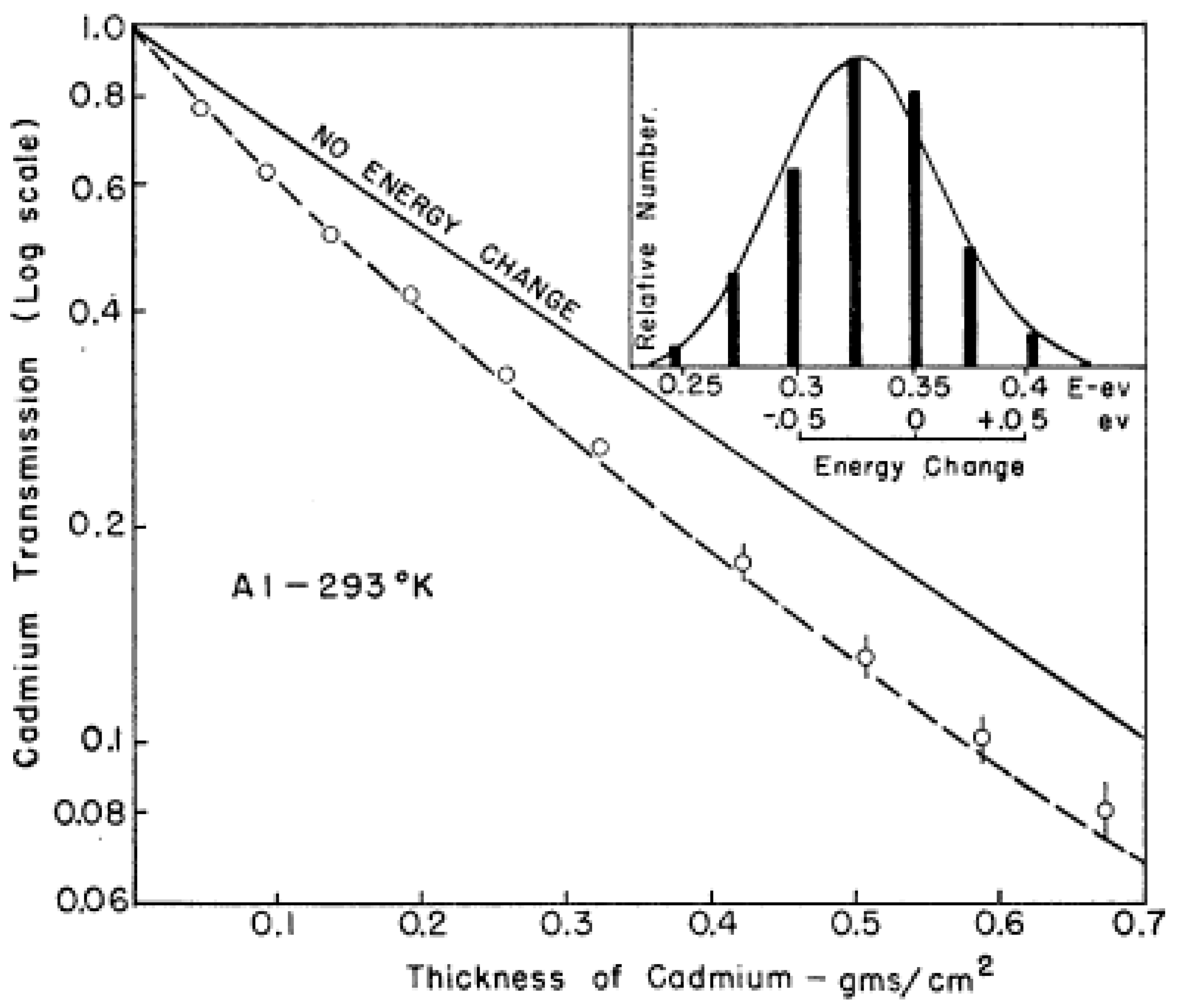
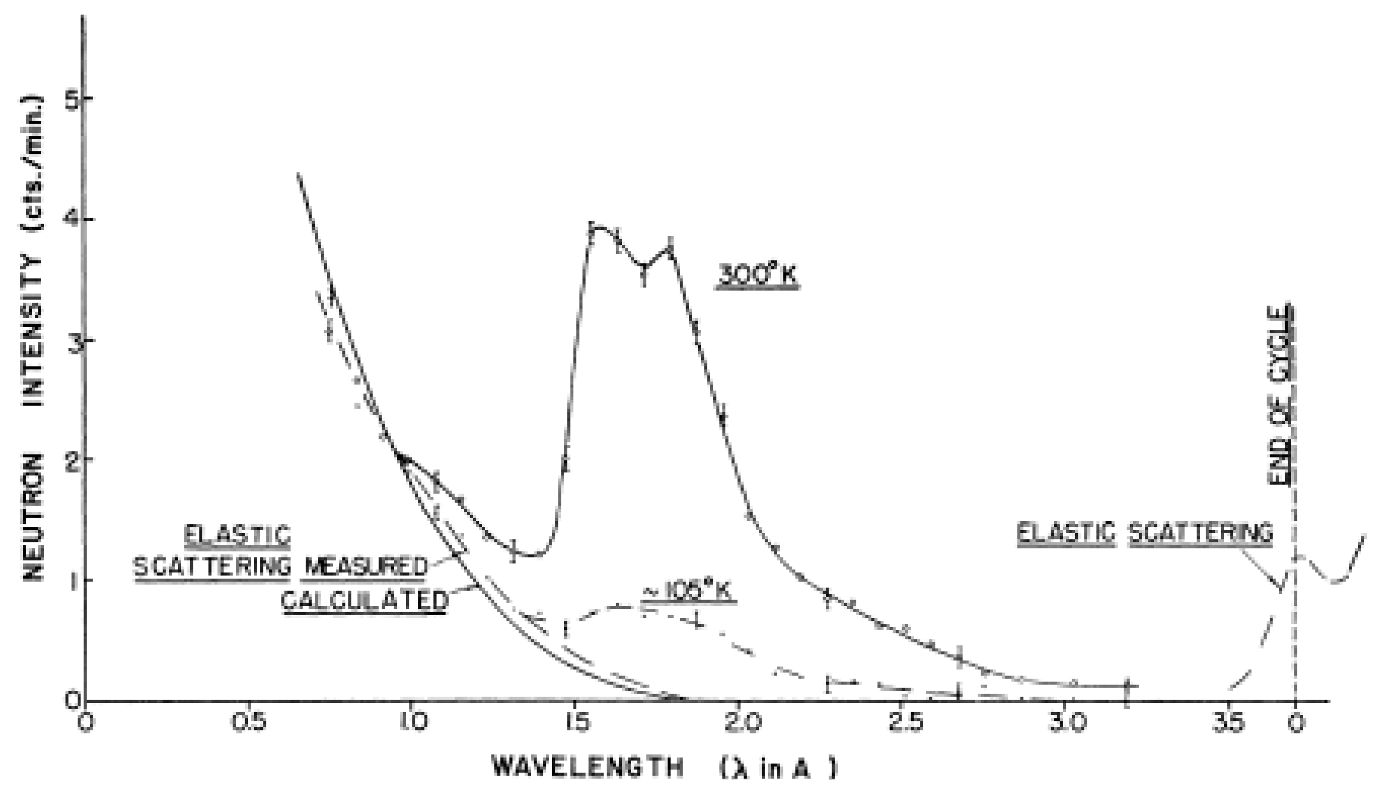
A major insight [15] by Brockhouse and Hurst into inelastic neutron scattering resulted from the resonant absorption measurements on Cd [13] and confirmed that the suspected deviations from the Breit–Wigner form originated in inelastic scattering by the atoms. The one-to-one correspondence observed in Cd near 350 meV, between the intensity of transmitted neutrons and the neutron wavelength, lead to its use as an analyzer to test the average wavelength of the neutrons scattered by Pb, Al, and C. The significance of the method was recognized by Brockhouse in his Nobel address [2]. The apparatus was similar to that used for the resonant cross-section measurements [13] except that Pb or Al or C replaced Cd as the scattering sample, and up to ten different thicknesses of Cd covered the cylindrical opening, illuminating the six symmetrically arranged BF3 counters. The incident neutron energy was 350 meV. The intensity transmitted by the Cd was measured for each of the ten thicknesses. The Cd transmission for the Al sample is shown in Figure 3. The solid line in the body of the diagram corresponds to zero energy change on scattering, and the open circles indicate the actual transmission and correspond to a net increase in neutron energy upon scattering. The deviation from the solid line increases in the order Pb, Al, C, corresponding to larger energy transfers as the mass of the scattering nucleus decreases.
The transmission was calculated on the basis of an Einstein model of the vibrational energy levels of a monatomic solid [15] (as well as for a gas of atoms obeying Maxwell–Boltzmann statistics) with Einstein temperatures, for Pb, Al, and C of 5.65, 25.9, and 150.0 meV. The Einstein vibrational levels for Al, with their characteristic separations equal to the Einstein temperatures are shown in the inset to the diagram. The model gave a satisfactory account of the net change in wavelength on scattering from these materials. Therefore, it gave a method of correcting measurements on resonant scatterers for inelastic neutron scattering, which was the original motivation. However, much more significantly, it suggested that the possibility of measuring energy transfers directly was close to being feasible. Previous work on the scattering of slow neutrons by polycrystalline materials had indicated a change in energy on scattering [16], but the large number of possible multiple scattering events in polycrystals and the ambiguity in the wavevector of the excitation had precluded any comparison with theory.
A complete account of the resonant scattering measurements on Cd, Sm, Gd, Eu, Dy, Rh, and In was given in [17], which extended and improved the earlier experiments [13,14]. Use was made of the Einstein model of solids [15], which had been shown to be adequate to account for the average energy change due to inelastic scattering surmised to be occurring previously. The incoherent scattering from V was used to calibrate the cross-sections and found to be 5.07 ± 0.15 bn, which is within the experimental error of the accepted value [10] of 5.10 ± 0.06 bn. The absorption cross-section was found to be 5.29 bn, which is slightly higher than the accepted value of 5.08 ± 0.04 bn. The work was characterized by careful attention to detail with respect to the small corrections to the raw data for self-absorption in the scattering sample, counter sensitivity as a function of scattering angle, diffuse scattering from the NaCl monochromator, and most importantly, for the change of wavelength on scattering. Discrepancies were noted between measurements of the total scattering cross-sections of Cd and Sm from other laboratories, which were subsequently found to be in error by of order 10%. The cross-section for Cd was shown to be consistent with a single resonance in Cd113 with spin 1 and for Sm with a single resonance in Sm149 with spin 7/2. Gd had contributions from two resonant isotopes. For Dy, the ratio was 0.2, which is too large for the approximations made in the analysis to be accurate. The resonances in Rh and In were at energies of 1260 and 1450 meV, which were well outside the accessible neutron energies available for the experiment.
An epochal meeting was held in December 1950 which formed the basis of the success at Chalk River in inelastic neutron scattering and indeed the Nobel Prize for Brockhouse. In his lecture at the conference [6] celebrating the 50th anniversary of the discovery of the neutron, he said: “The genesis of the Idea at Chalk River came in a study-group meeting in December 1950 in which D.G. Hurst, G.H. Goldschmidt, N.K. Pope, and myself participated. (The idea is known to have germinated elsewhere at about the same time.) The decision was made that the experiments were feasible with the NRX reactor, then in operation for several years.” R.A. Cowley in his biographical memoir of Brockhouse [18] filled in some further details of the meeting: “It was in 1950 that a meeting of Don Hurst, Bert, Neville Pope, and G. Goldschmidt decided that the resolution of the instrument could be improved only if the energy of the incident and scattered neutrons was reduced and that such experiments should be possible with the NRX reactor at Chalk River, which at that time had the highest neutron flux in the world. Nevertheless, these experiments would require, in addition to this high flux, considerable advances in the experimental techniques.” Finally, in the Acknowledgements in the seminal paper on the normal modes of aluminum by neutron spectroscopy [19], the authors stated, “The authors are indebted to Dr. G.H. Goldschmidt, Dr. D.G. Hurst and Dr. N.K. Pope for a conversation in 1950 which lead to the design of these experiments and to Dr. Hurst and Dr. Pope for many discussions since.”
3. The Period Prior to the Invention of Constant-Q (1951–1957)
3.1. Lattice Vibrations in Aluminum
The first ever measurements of lattice vibrations in a solid by neutron inelastic scattering were reported in 1955 [20]. It had been realized in principle for about five years that such measurements could be done, and this paper was the experimental achievement of the discussions held at Chalk River some four years previously. Bragg diffraction is far stronger than phonon scattering, but when the experimental arrangement is such as to avoid single-crystal diffraction, then the weaker inelastic scattering can be observed. It was noted that an experiment to measure phonons in Al was tried unsuccessfully at Chalk River in 1952.
If k and k′ are the initial and final neutron wavevectors, Q = k − k′, is the wavevector transfer or scattering vector, q is the phonon wavevector, and τ is a reciprocal lattice vector, then wavevector conservation between the neutron and the phonon may be written,
k − k′ − 2π τ + q = 0.
In addition, the neutron–phonon system must conserve energy, so
where m is the mass of the neutron, E and E′ are the kinetic energy of the incident and scattered neutron, and νj is the frequency of the phonon in the jth normal mode. When these two conditions are met, a peak may be seen in the scattered intensity plotted as a function of the final neutron energy, E′, or the energy transfer to the crystal, E–E′. For a monotonic lattice, the frequencies are expected to separate into three branches, corresponding in the low-frequency limit, to the familiar longitudinal and two transverse sound waves.
E − E′ = (ħ2k2/2m) − (ħ2k′ 2/2m) = hνj
(The bold type in this article indicates the vector character of the symbol. Unit vectors are represented by a caret over the symbol, for example, .)
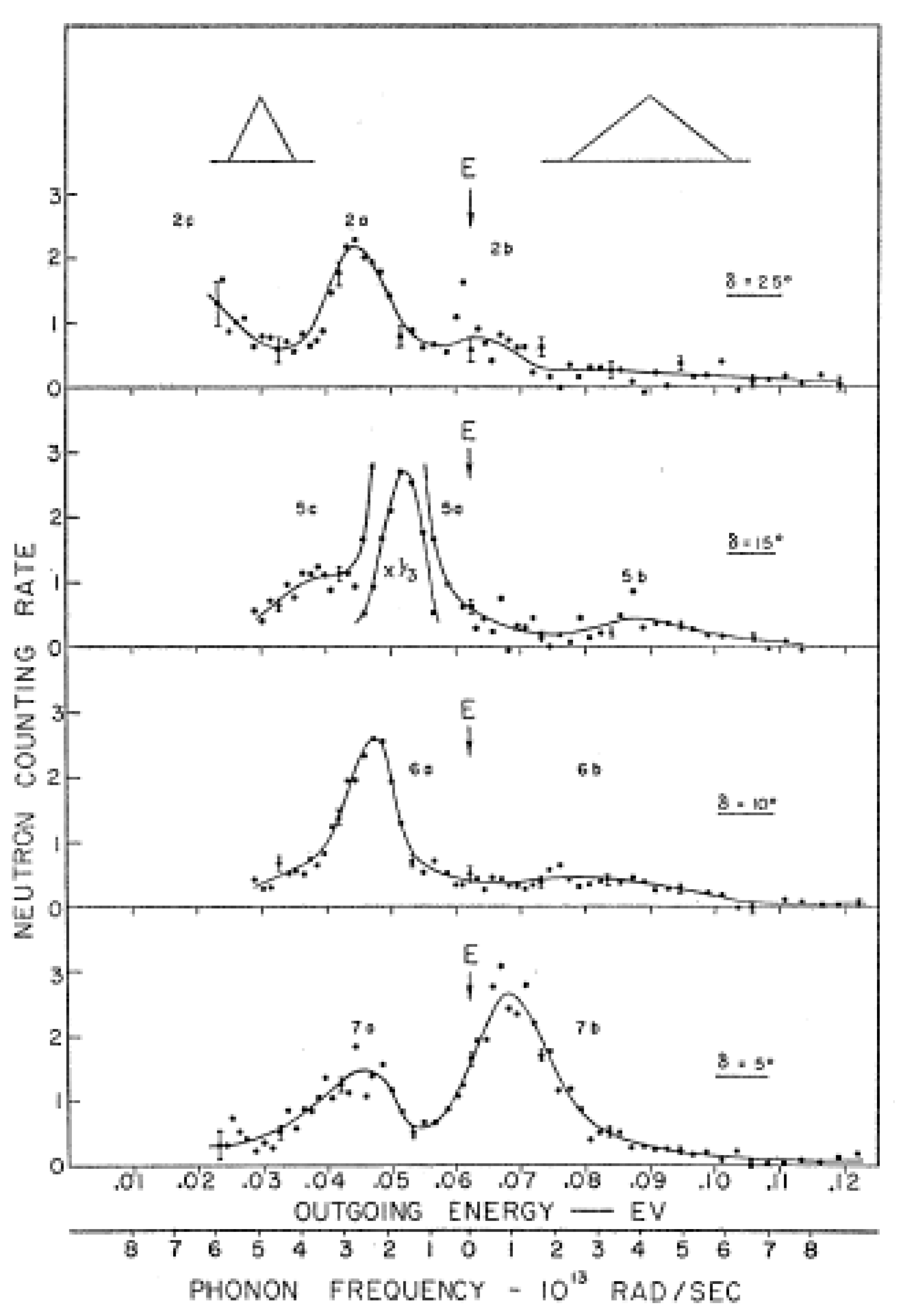
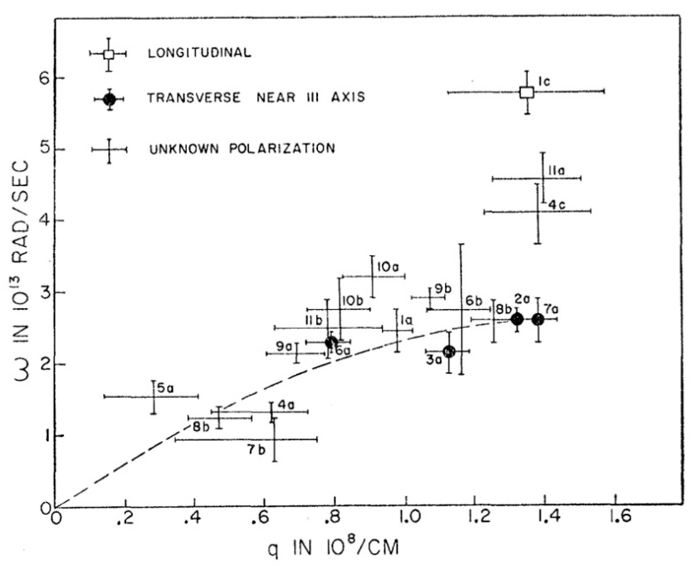
In the experiment, neutrons of constant wavelength 1.148 Å (62.2 meV, 15.0 Thz) from a crystal spectrometer fell on an aluminum crystal with a [] vertical axis. The Bragg angle, Φ = 2θB, for scattering from the (333) reflection when the [111] direction is along the scattering vector, Q, is 95.1°. Measurements were made with the crystal angle rotated by increments, δ, from the angle, ΨB, the angle between the [002] axis of the crystal, and the incident wavevector, kB, for Bragg scattering. The energy distribution was measured with a second crystal spectrometer, thus constituting a rudimentary triple-axis crystal spectrometer. The set-up with fixed E and variable E′ is equivalent to a chopper spectrometer with fixed incident energy and variable scattered energy determined by the time of flight of the neutrons from the sample to the counter. Then, it is difficult to be sure which phonons will satisfy the energy and momentum conditions or whether they will be in high symmetry directions. Sometimes, the branch of phonons, transverse acoustic (TA) or longitudinal (LA), could be assigned, but often, they are not. Since these were the first recorded phonons, the scattered neutron intensities, referred to as neutron groups, as well as the first experimental ν(q) dispersion relation are shown in Figure 4 and Figure 5. Four points on the TA branch were established and one was established on the LA branch, but the remainder were of unknown polarization. The position of the TA phonons matched a sinusoidal curve with an initial linear slope corresponding to the transverse velocity of sound in aluminum. The authors noted that similar inelastic neutron scattering experiments were being carried out by Jacrot in Paris [21] and by Carter et al. at Brookhaven [22].
A complete series of experiments on the lattice vibrations in Al was reported by Brockhouse and Stewart in 1958 in their epochal paper in Rev. Mod. Phys. [19]. An enormous amount of ground was covered in the three-year intervening period in obtaining the phonon dispersion relations in several high-symmetry directions. The observed results were in agreement with the cross-section and selection rules for one-phonon and two-phonon processes. Two different crystals were examined both by crystal and time-of-flight spectrometry. The various processes that give accidental sharp peaks that masquerade as excitations and are usually referred to as “spurions” were identified. Reasonable error estimates were made, and preliminary estimates of the resolution were obtained. Finally, the results were discussed in terms of the existent theories of lattice dynamics and compared with the results of diffuse X-ray experiments. That is, all possible checks were made to establish that the inelastic scattering observed was due to lattice vibrations.
At this point, it is worth making the explicit connection between the phonon frequencies and the force constants between the atoms in the crystal. In the Born–von Kármán theory of lattice dynamics [23], the crystal is considered as a system of mass points that interact with forces obeying Hooke’s Law. The equation of motion in the general case of more than one atom in the unit cell is
where mκ is the mass of the atom of type κ in the l th unit cell, ux is the displacement of the atom from equilibrium in the x direction, and Φxy(κκ′:ll′) is the force in the direction x on the κth atom in the lth unit cell when the κ′th atom in the l′th cell is moved one unit distance in the y direction. The Φx,y are the interatomic forces of interest. The solutions to the equation of motion are plane waves of frequency, υ, wavevector, q, and polarization vector, U(q), where all wavevectors q within the Brillouin zone of the reciprocal lattice are permitted.
For one atom per unit cell, the equation of motion reduces to
where
and are components of the polarization vector, U(q), in three selected orthogonal directions, Rl is the vector distance of the atom in cell l from the given atom, and Φαβ(Rl) is the force on any given atom in the α-direction when the neighbor at Rl moves a unit distance in the β-direction. The generalization to the cases where there are more than one atom per unit cell is straightforward and has been given in detail in [24]. The equation only has a solution for when the frequency satisfies the determinantal equation
which has three eigenvalues where j denotes the branch of the frequency spectrum. For each value of q, there is a polarization vector, an eigenvector, whose components satisfy Equation (7) above.
When q lies in a mirror plane, for example the plane of a cubic crystal, one may take one component of the polarization vector, say U3, in the z-direction along the plane normal, and then the other two components, U1 and U2, must lie in the plane but are otherwise not fixed. Then, the determinant, Equation (7), factors into two equations, namely for j = 3
and for j = 1 or 2
If q lies in a second mirror plane, U1 and U2 are also fixed by symmetry, = 0, and Equation (9) also factorizes. Then, the squares of υ1 and υ2 are also linear in the force constants, which may then be fitted by linear least squares methods to the squares of the frequencies. For these cases, the equations may be written in terms of interplanar force constants, which are equivalent to the forces along the length of a simple linear chain, as was pointed out by Foreman and Lomer [25]. The equation for one direction may be written
and it is useful, since it permits an estimate of the spatial extent of the interatomic forces operating in the crystal structure, which depend strongly on the electronic structure.
The cross-section for the one-phonon process per 4π steradians per nucleus per second integrated over energy is given by Equation (4) of reference [19],
σcoh and m are the coherent cross-section and mass of the scattering nucleus, and e−2W is the Debye–Waller factor. The temperature factor Nλ is given by
Nλ = [ehν/kT − 1]−1.
For phonon creation, neutron energy loss, the intensity is proportional to Nλ + 1, and for phonon annihilation, the intensity is proportional to Nλ. The Jacobian factor is
where ε = 1 for neutron energy loss and −1 for neutron energy gain. The cross-section is summed over the number of phonon modes contributing to one neutron group, which simultaneously satisfy the conservation conditions, Equations (2) and (3).
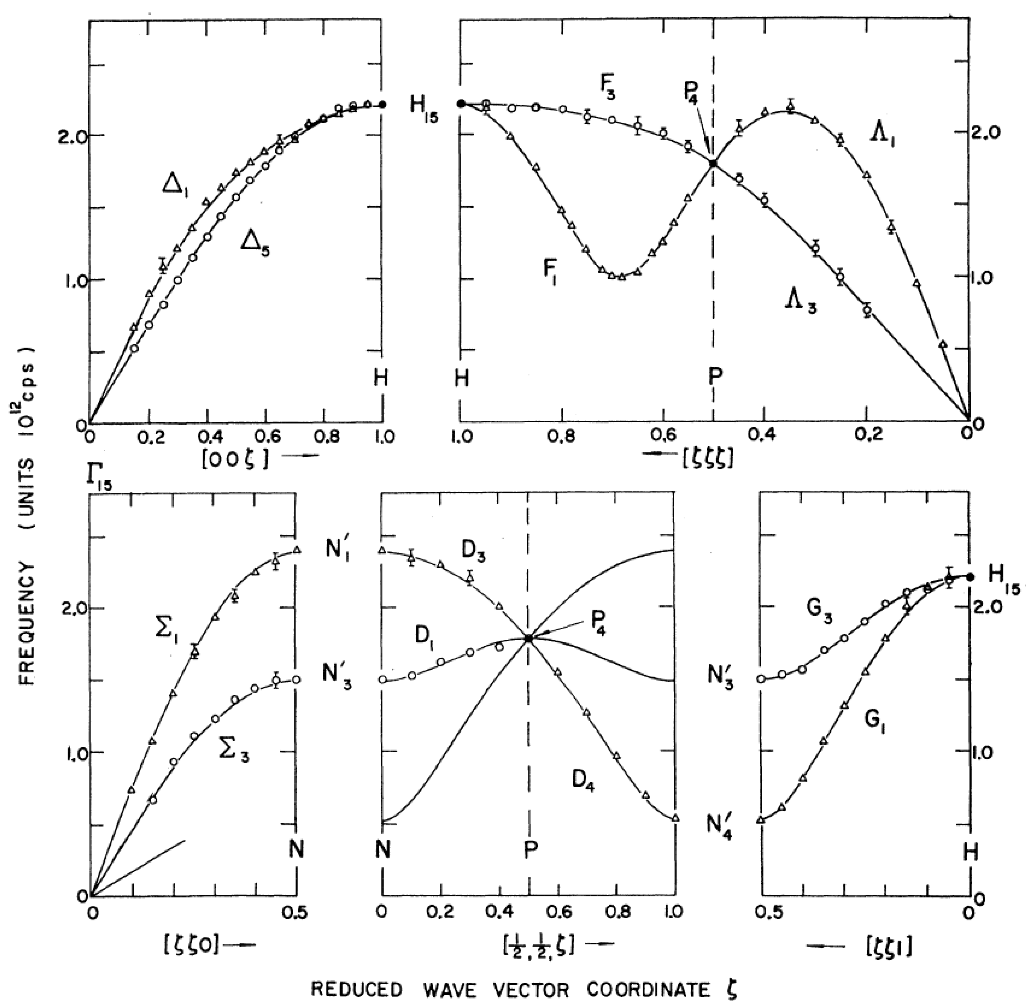
The phonon experiments were carried out at the NRX reactor (intensity in the core 3 × 10¹² neutrons per cm−2 s−1) at Chalk River on two crystals of Al oriented with [] or [100] vertical axes with either a crystal spectrometer equipped with Al monochromators defining the incident and scattered beams or with a filter-chopper. With the crystal spectrometer set-up, the background from cosmic rays or fast neutrons coming down the incident beam or through the shielding was measured by turning the analyzer crystal off its Bragg position. The resolution in k and k′ was estimated from the collimator geometry and the mosaic spreads of the monochromating crystals. The incoherent scattering from vanadium at the elastic position gave the energy resolution.
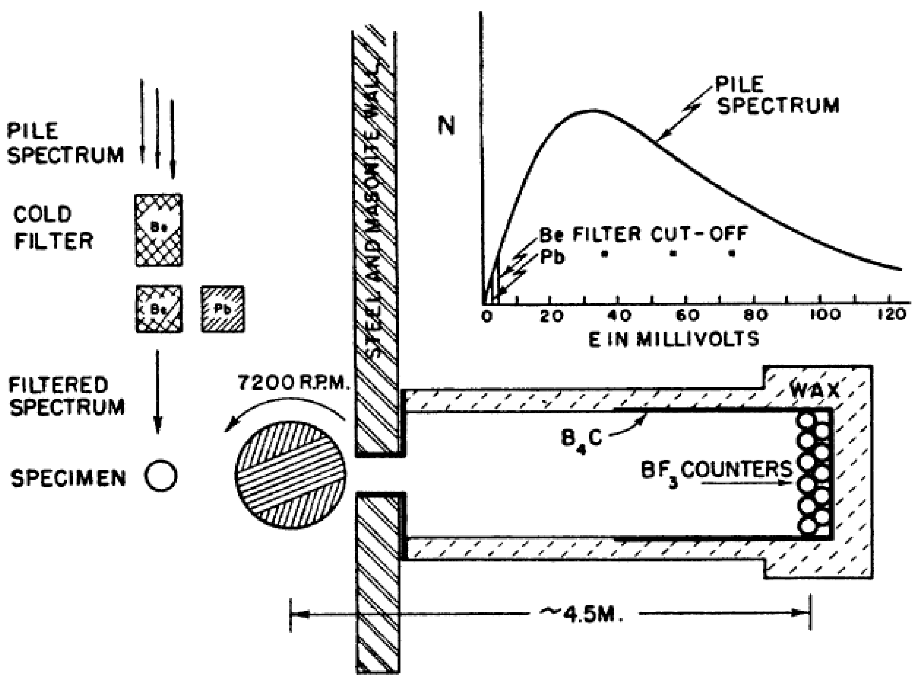
The filter-chopper equipment [19] is shown in Figure 6 and uses neutrons with an average wavelength of 4.0 Å obtained by the difference count between a beryllium filter with a Bragg cut-off of 3.96 Å and a lead filter with a cut-off of 5.07 Å. Therefore, the incident wavevector, k, is short. The difference count also serves to subtract the fast neutron background. The velocities of neutrons scattered at Φ = 90° were measured with a simple Fermi chopper which produces 240 pulses per second, with width in time of 140 μs. The time to traverse the 4.45 m flight path to the counter permits the scattered energy E′ to be measured. The scattering process is neutron energy gain by phonon annihilation. The energy resolution of the set-up was of order of the width of the observed neutron groups.
In the original crystal spectrometer experiments [20] with fixed incident energy of 62.2 meV (1.148 Å) and scattering angle Φ = 95.1°, measurements were made in both neutron energy gain and loss in Brillouin zones containing the (115), (224), (333), and (442) reflections. New measurements were made with a scattering angle of Φ = 88.0° in the (222) zone. To make doubly certain of the results, higher resolution measurements were made with an incident energy of 35.1 meV (1.523 Å) in 10 different Brillouin zones. In this series of experiments, spurious sharp peaks were obtained, which originated from second-order reflections (λ′/2) in the analyzer crystal. Further spurious peaks were identified as coming from second-order neutrons in the incident beam (λ/2 = 0.761 Å, E = 140.4 meV), which were Bragg scattered by the (355) reflection of the sample and observed in second order in the analyzer. By this time [19], the crystal spectrometer had been modified so that the scattering angle, Φ, and the crystal angle, Ψ, could be accurately set on angular scales. Then, Φ and Ψ could be set up to a first approximation if ν and q were specified. Then, this process was iterated to obtain values of q close to symmetry directions.
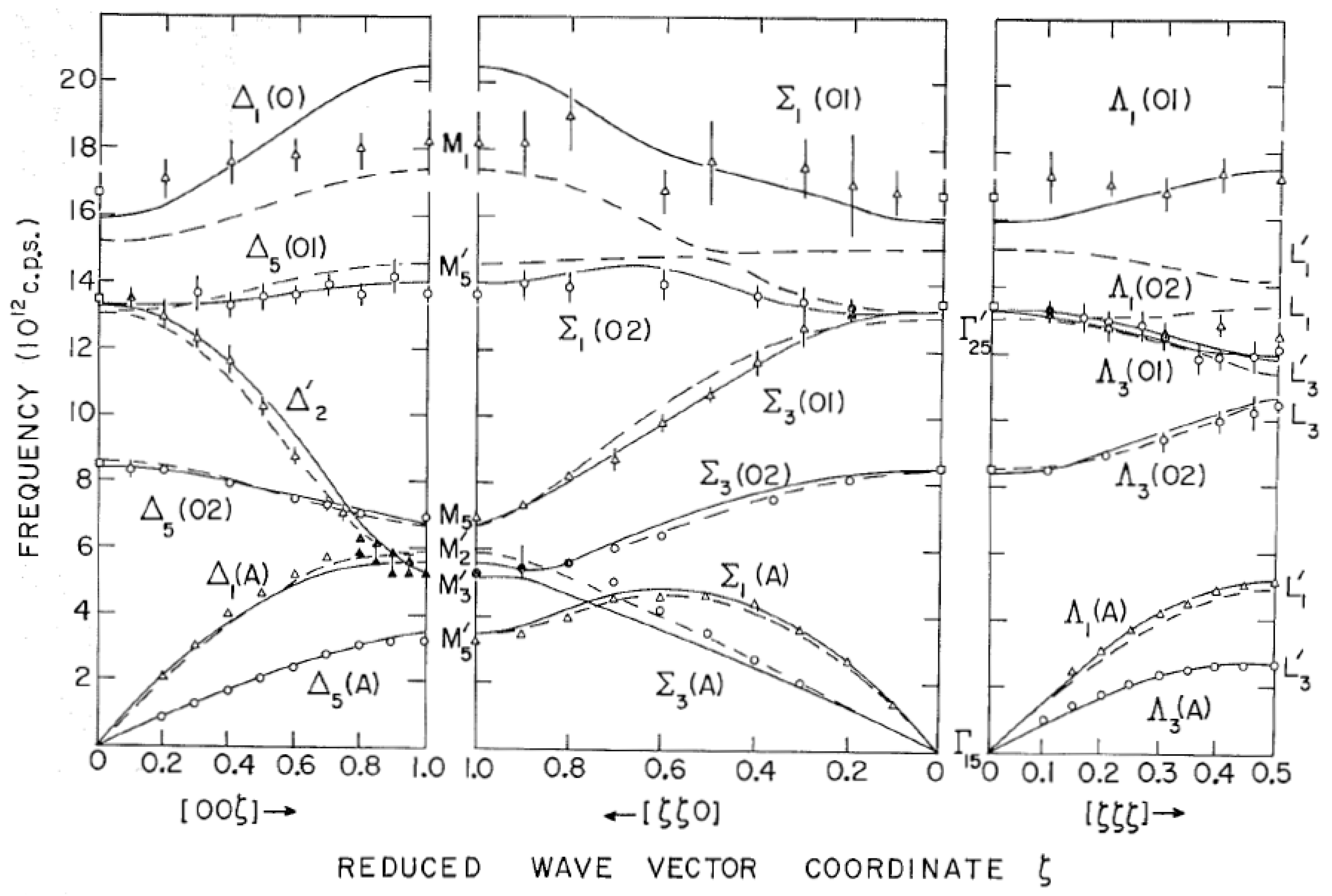
Measurements were made with the filter-chopper spectrometer in the (001) plane of Al to obtain the branches not observable in the () plane, namely the transverse acoustic [110] mode with displacement in the [] direction. With these overlapping datasets, the ν(q) dispersion relation was plotted for the [ζ00], [ζζ0], and [ζζζ] directions. The data showed that the phonon intensities were largest near the reciprocal lattice points varying such as kT/ν2 at relatively high temperatures, as given by Equations (11) and (12).
The factor [Q.Uj]2 in Equation (11) is a selection rule for the intensities of the phonons. In the () and (001) mirror planes, one of the polarization vectors has to lie perpendicular to the mirror plane, i.e., along the [] and [001] directions, respectively, while the other two polarization vectors have to lie in the respective planes. Only the transverse mode in the plane is allowed because of the selection rule. However, the TA phonon with [] polarization can be seen in the (001) plane. For [100] phonons, the transverse displacements in the [010] and [001] direction are equal, so the TA modes are degenerate.
3.2. Lattice Dynamics of Germanium, Silicon, and Diamond
As a result of its interest as a semiconductor, many properties of Ge in which the lattice vibrations play a part had been studied, so that a mapping of the frequency-wavevector relation was important. The normal modes of vibration were presented as a letter and later a more complete paper by B.N. Brockhouse and P.K. Iyengar [26,27]. The diamond-type lattice of Ge is the simplest case of more than one atom per unit cell and therefore offers the possibility of measuring both the acoustic and optic modes. In Ge, the elastic constants nearly satisfy an identity which suggests that the force constants might be restricted to first neighbors alone. In fact, Hsieh [28] had calculated the normal modes based on this assumption, although the calculated values were in disagreement with infrared absorption-edge measurements.
For a crystal with n atoms per unit cell, there are 3n branches of the spectrum; three branches are acoustic, for which ν goes to zero as q goes to zero, and 3n − 3 are optical branches, longitudinal LO or transverse TO, where ν is finite at q = 0. In special directions, [111] and [001], in a mirror plane, the normal modes are strictly transverse or longitudinal. For q in a mirror plane such as (), there are two branches with polarization vectors normal to the plane and four branches with eigenvectors in the plane. The scattered neutrons occur in groups satisfying Equations (2) and (3). In the Born–von Kármán theory, the frequencies ν2 are eigenvalues of a 3n × 3n determinant, which in symmetry directions factorizes into n × n and 2n × 2n determinants, making the calculations simpler. The cross-section for the creation or annihilation of one phonon integrated over energy is similar to Equation (11)
For the [001] and [111] directions, where the polarization vectors for both atoms are in the same direction, the structure factor, gj (q, τ), which is a generalization of (Q.Uj)2 in Equation (11), may be written for the four branches visible in the plane as
where is the scalar magnitude of the polarization vector for the k = 1 atom in the unit cell. The structure factors calculated from the Hsieh [28] approximation to the force constants showed where in the reciprocal lattice the LA, TA, LO, and TO modes were most intense.
The crystal spectrometer [4] at the NRX reactor provided the incident beam of fixed wavelength, and a second spectrometer using the (111) plane of Al analyzed the scattered neutron beam. As in the previous Al experiments [19,20], the magnitude of the incident wavevector, k, was fixed, and the scattering angle and crystal angle were varied to locate the phonon frequencies near the symmetry directions around various reciprocal lattice points, τ. Once an estimate of the phonon frequency was found, it was straightforward to alter the conditions slightly to come closer to the symmetry direction.
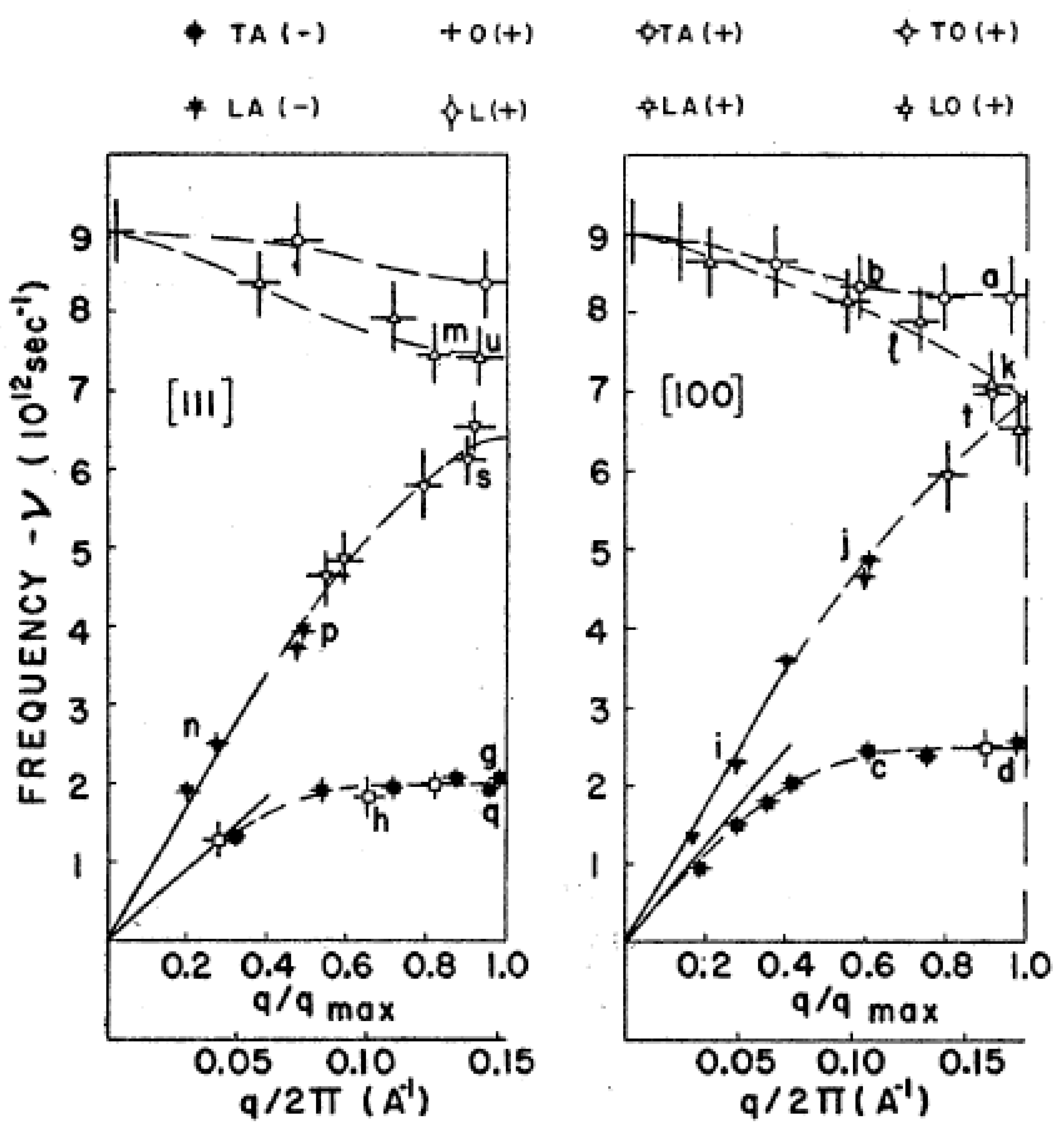
The frequency versus wavevector dispersion relation in the [111] and [100] directions is shown in Figure 7 for a single crystal of Ge aligned with [] vertical axis at 20 °C. The [100] TA branch was observed near the (400) reciprocal lattice point where the polarization vector is along [110], while the LA branch was observed beyond the [006] reciprocal lattice point where the polarization vectors are along [001]. The TO was observed in the Brillouin zone containing the [551] reciprocal lattice point where the preliminary structure factor calculation showed the TO mode to be strong because of the factor. The measured frequencies, particularly the TA phonon mode, disagreed with Hsieh’s model [28] by 50% at the [111] zone boundary, but they agreed with infrared absorption measurements. The inclusion of 2nd nearest neighbors in a Born–von Kármán model still left a 25% discrepancy. The discrepancy was important, since it suggested that some essential physics was missing, and this lead eventually to the shell model. Peaks in the far-infrared absorption coefficient in Ge were readily explained as two-phonon summation bands at 77 K and three-phonon bands at 300 K.
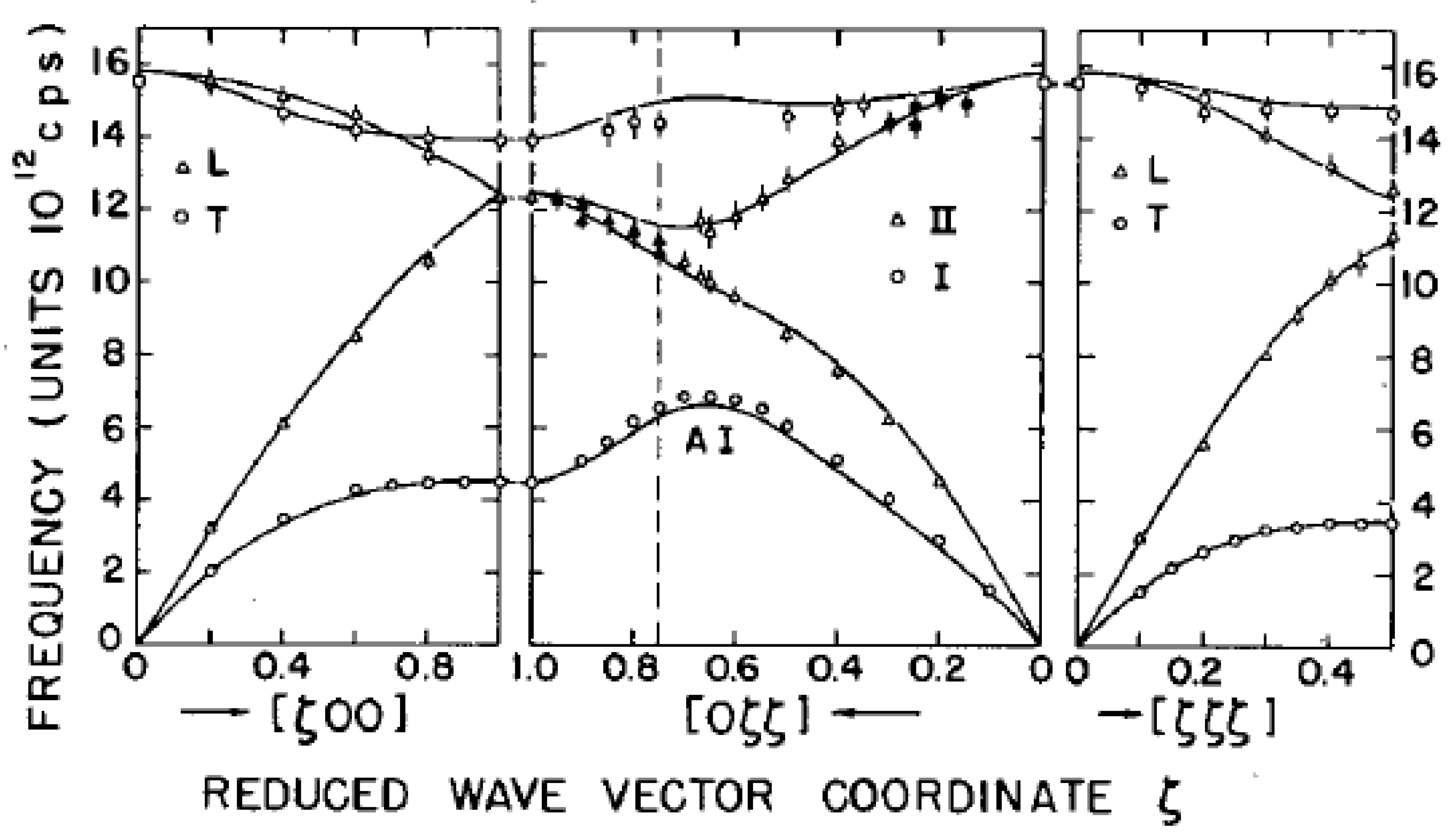
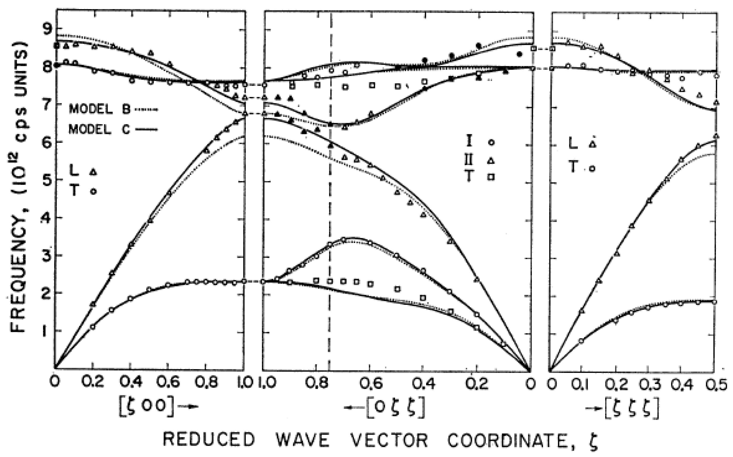
The experiments by Brockhouse [29] and by Dolling [30] on silicon, which has the same electronic structure as germanium, and the discussion by Dolling [30] on the shell model naturally follow the above discussion although some years later. Brockhouse found that the frequencies of silicon were at the same wavevector as germanium in the [00ζ] direction, scaled by a factor 1.73 ± 0.04, so that an inability to describe germanium with the Born–von Kármán model also applies to silicon. The shell model had been developed by Dick and Overhauser [31] to deal with the dielectric properties of the alkali halides. In the model, an atom is imagined to consist of a core, the nucleus and inner electrons, and a spherical shell of outer electrons of zero mass. During a lattice vibration, the cores and shells are relatively displaced, and the resultant dipoles exert a long-range force on each other. The shell model specifically developed by Cochran [32] to explain the neutron results in germanium introduced core–core, core–shell, and shell–shell force constants between nearest neighbors and also permitted a theoretical description of the dielectric properties. The model [30,32] showed that the nearest neighbor shell model resolved the discrepancies between experiment and the rigid atom calculation for the [ζ00] and [ζ ζ ζ] directions although not for the [ζ ζ0] direction. By introducing an additional two next-nearest force constants [30], further improvements were made to the fit. The most complete shell model fit (IIC), as shown in Figure 8, included an antisymmetric force constant, which only contributed in the [ζζ0] direction. However, Dolling pointed out that the next-nearest-neighbor force constants were only a few percent of the near-neighbor constants so that the crucial physics was including the shell model to the nearest neighbors. In 1967 [33], the complete phonon dispersion relation of diamond, the Oppenheimer Diamond, was measured on the Omega-West reactor at Los Alamos National Laboratory, which had an enhanced flux of relatively high energy thermal neutrons and was necessary to measure the optic modes at an energy of about 125 meV. Collaborating with the Los Alamos group, Dolling and Cowley obtained an accurate description of the phonons with the shell model developed at Chalk River for Ge and Si and included a next nearest neighbor force constant as in the case of Si.
3.3. Incoherent Scattering and the Phonon Density of States, g(ν)
The frequency distribution of normal modes of a crystal lattice, g(ν), is determined by the atomic forces and structure of the crystal. An experimental measurement of g(ν) can be made by measuring the incoherent nuclear inelastic scattering. Of the elements, only V has a sufficiently small coherent cross-section to make this possible (σcoh = 0.018, σinc = 5.10, σabs = 5.08 bn). By alloying Mn and Co together for a concentration of 0.42, the average coherent cross-section can also be made small, namely (σcoh = 0.007, σinc = 4.08, σabs = 26.7 bn). The theory of incoherent inelastic scattering was given by Cassels [34]. A slow neutron may be scattered inelastically when a neutron excites or de-excites one phonon or more than one phonon (multiphonon) modes. For an incoherent scatterer, the momentum change of the neutron does not impose any conditions on which phonon modes are excited. Then, the probability that a neutron changes its frequency by energy hυ is proportional to the number of vibrational modes between and + d .
The inelastic scattering cross-section can be written for neutron energy gain
where m is the mass of the scattering nucleus, and k, E are the initial neutron wavevector magnitude and energy, and the primed quantities are the final values. The measurement of a scattered neutron intensity is much more difficult than that of the frequency of a neutron group, since it has to be corrected for various instrumental and intrinsic backgrounds as well as for instrumental artifacts.
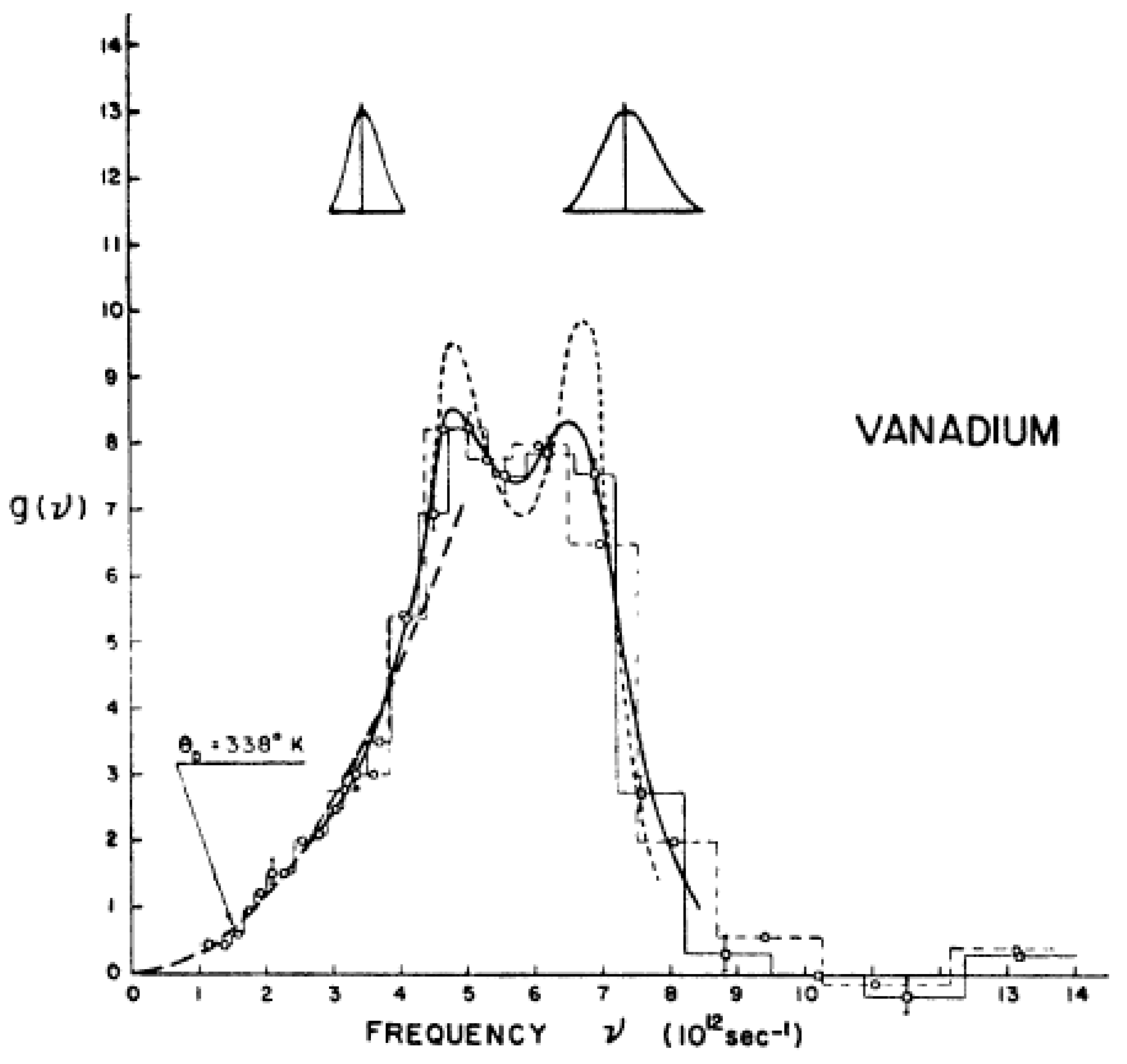
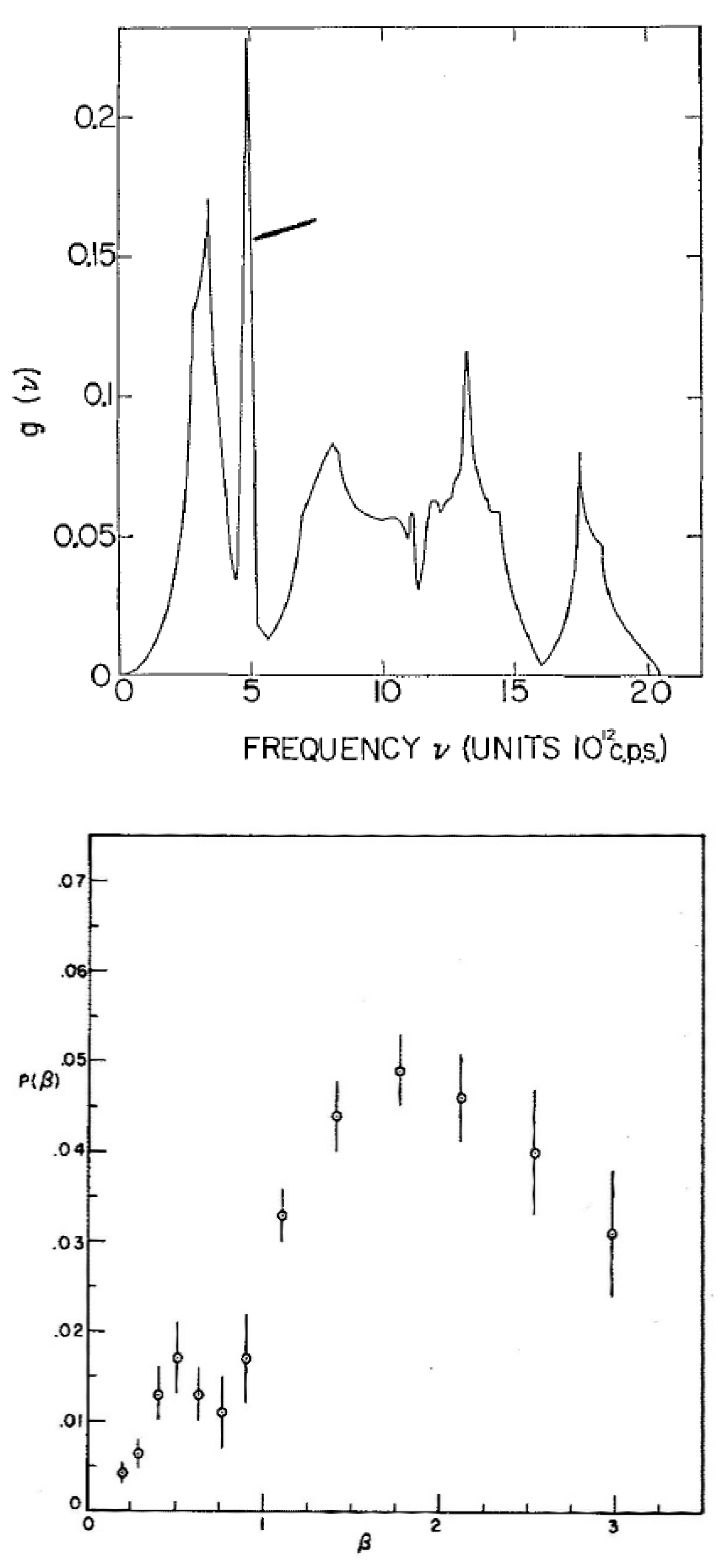
The neutron scattering measurements [35] were made by time of flight in neutron energy gain. The incident beam, filtered alternately through cooled Be or Pb (Bragg cut-offs of 3.96 and 5.70 Å, respectively) had an average energy of 4.0 meV and width of 2.5 meV. The neutrons were scattered through 90° at the sample through a Fermi chopper into a bank of twelve BF3 counters. The Be-Pb difference pattern as a function of average scattered wavelength is shown in Figure 9. The region marked “elastic scattering” is a frame overlap from the previous burst of the Fermi chopper. The scattering centered near 1.8 Å is the inelastic scattering of interest. Corrections for chopper transmission, counter wavelength sensitivity, air attenuation, and scattering were made. The most troublesome correction is for multiple scattering, where a neutron creates or destroys two phonons in one scattering event or the annihilation of one phonon followed by the creation or annihilation of a second phonon in a second scattering event. The calculation of the two-phonon scattering requires the integration of the double phonon cross-section over the observed spectrum [36,37]. Both effects give intensity over the whole region of the one-phonon scattering. The corrected vibrational spectrum for V is shown in Figure 10. The low-frequency part of the spectrum matched a Debye spectrum corresponding to a Debye temperature, θD, of 338 K, as found from low-temperature specific heat measurements.
3.4. Structure and Dynamics of Liquid He4
The first preliminary neutron measurements from Chalk River on liquid He4 were reported by Henshaw and Hurst in 1953 [38], thus beginning a field of endeavor that continued for over half a century. The results corrected for background and the change of effective volume with scattering angle were accurate to ±7%, while double scattering and the effect of resolution were noted to be smaller than the statistical error. The main finding was the position of the first peak in the structure factor at 2.15 ± 0.0.11 Å−1. This peak was attributed to a peak in the radial distribution function, g(r), at 3.6 Å.
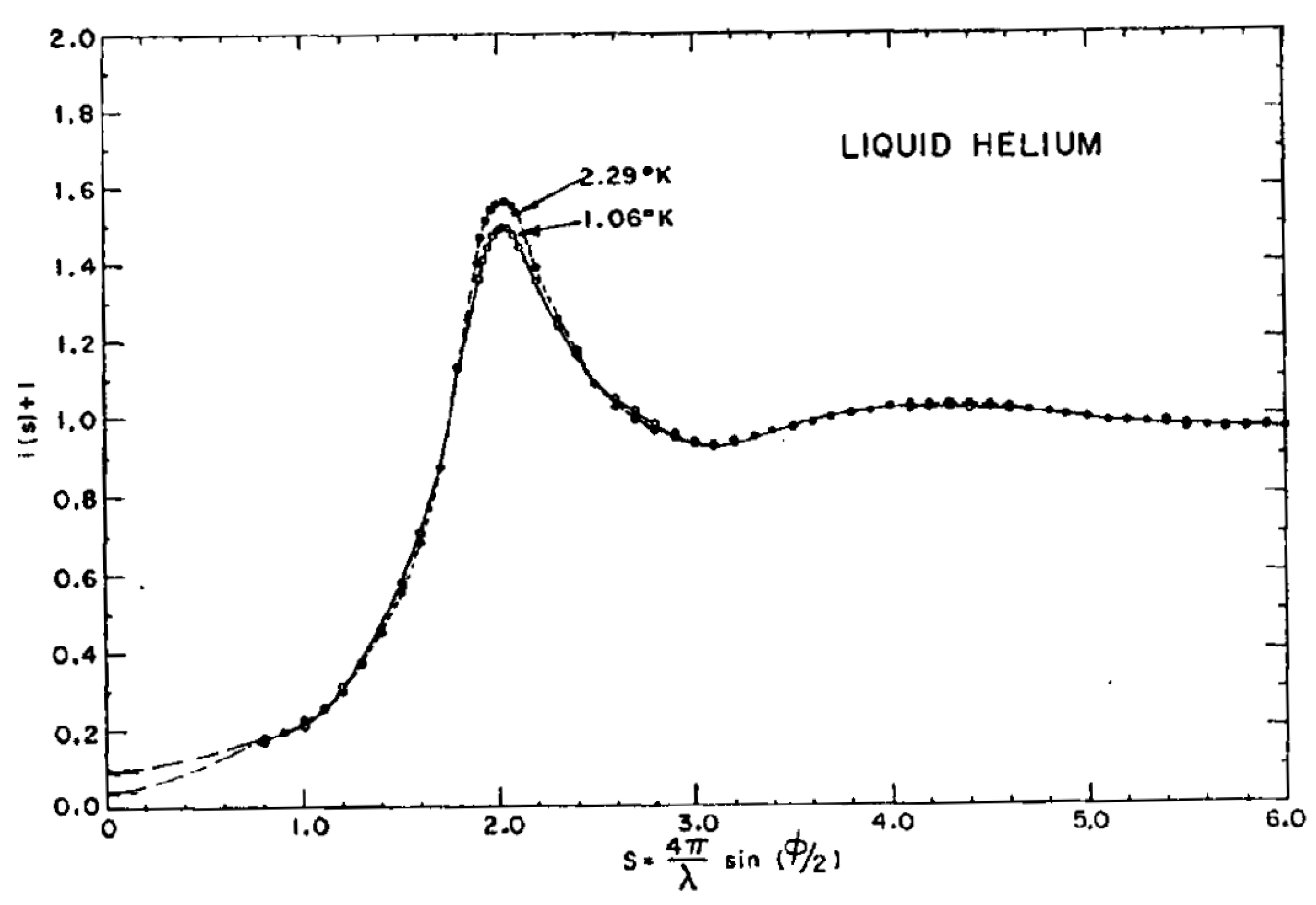
The experiments described in [39] are a continuation of the preliminary measurements reported by Henshaw and Hurst in 1953. The measurements were made in a He4 cryostat with a monochromatic beam of neutrons of wavelength 1.04 Å from an NaCl monochromator at temperatures of 5.04, 4.24, 2.25, 2.15, 1.95, and 1.65 K and covered a range of density from 0.095 to 0.145 gmcm−3. The scattering was measured for angles between 4 and 80° (Q between 0.42 and 7.77 Å−1). The angular resolution was taken to be the width of the KBr {002} diffraction peak, which is near the maximum in the structure factor. The results were corrected for ambient background, effective scattering volume in plate geometry, and instrumental resolution. The multiple scattering was calculated to be negligible. At large Q, the scattering would be expected to decrease in a similar way to the scattering from free atoms, i.e., in an uncorrelated incoherent way. The experimental points were divided by the differential cross-section of a free He atom and the result was normalized to make the average quotient unity at large angles, since g(r) is unity at large r and S(Q) is unity at large Q. The assumption inherent in this normalization is that most of the scattering is incoherent and that the coherent scattering that reveals the structure of liquid He4 is restricted to small angles and in the region of the peak in S(Q) around Q = 2.057 Å−1. The measured energy loss for scattering by a free He atom at the peak of the structure factor is 2 meV, which is small compared with the incident energy of 75.8 meV. Thus, the assumption that a diffraction measurement integrates over the inelastic spectrum is reasonable at 2.057 Å−1 although not at 6.04 Å−1, where the energy loss is 17 meV.
The principal result of the experiment was that the normalized results at temperatures below and above the λ-point show no change in the position of the first peak in Q, although the peak becomes more intense with respect to the normalized value of unity at high Q. That is, at this resolution, there appeared to be no change in the structure of He4 at the λ-point. This is not to be expected, since there is a change in the velocity distribution at the λ-point but no change in the spatial distribution. With the assumption that the normalization procedure captures the coherent scattering, the radial distribution function rρ(r)/ρ0 was calculated from S(Q) by Fourier transformation. While the radial distribution function shows spurious peaks below 2.5 Å−1 due to the finite Q-range of the data, a shell of neighbors around 3.8 Å and also departures from uniform density around 7 Å are observed. The area under the main peak corresponds to about eight nearest neighbors, which would be the case for a body-centered cubic material.
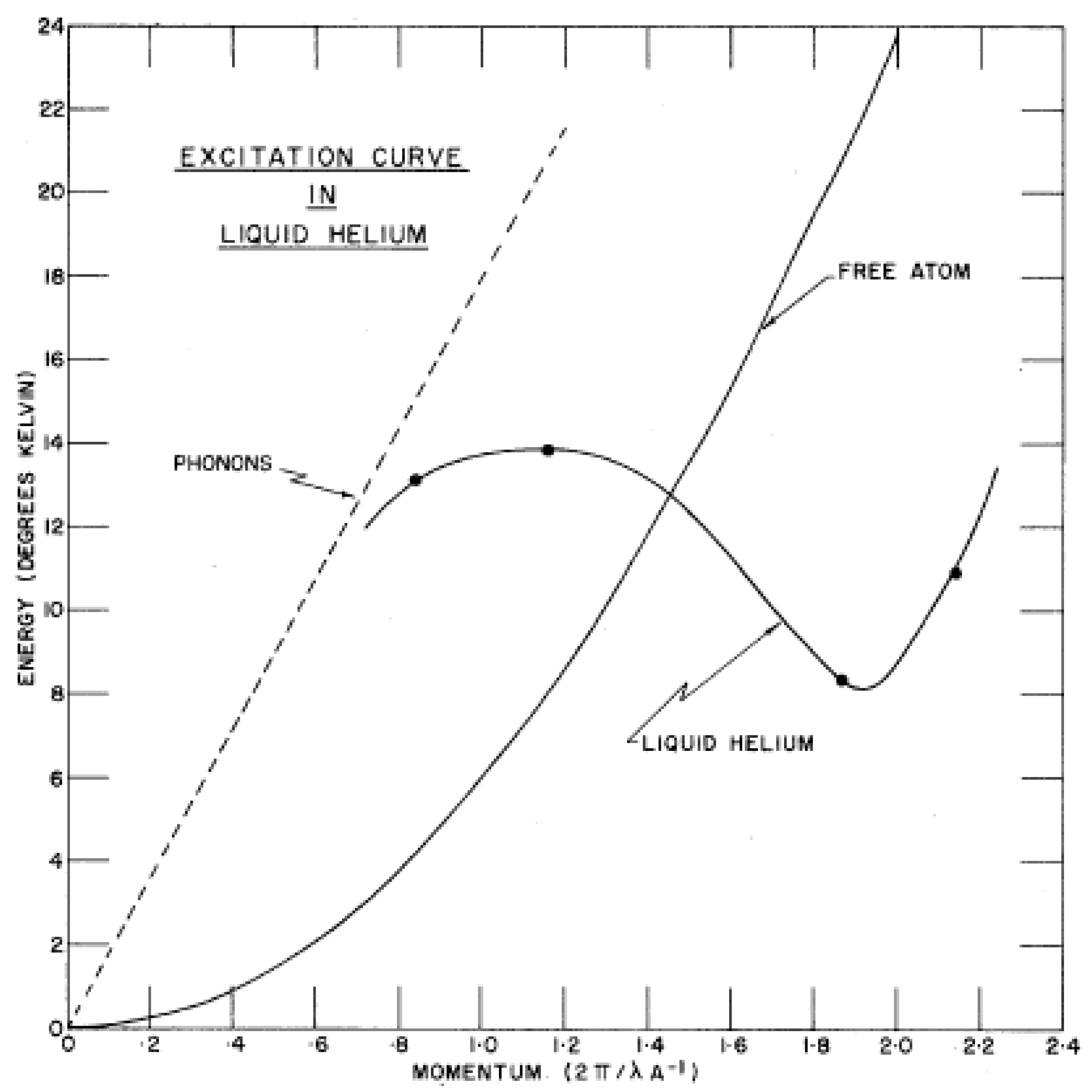
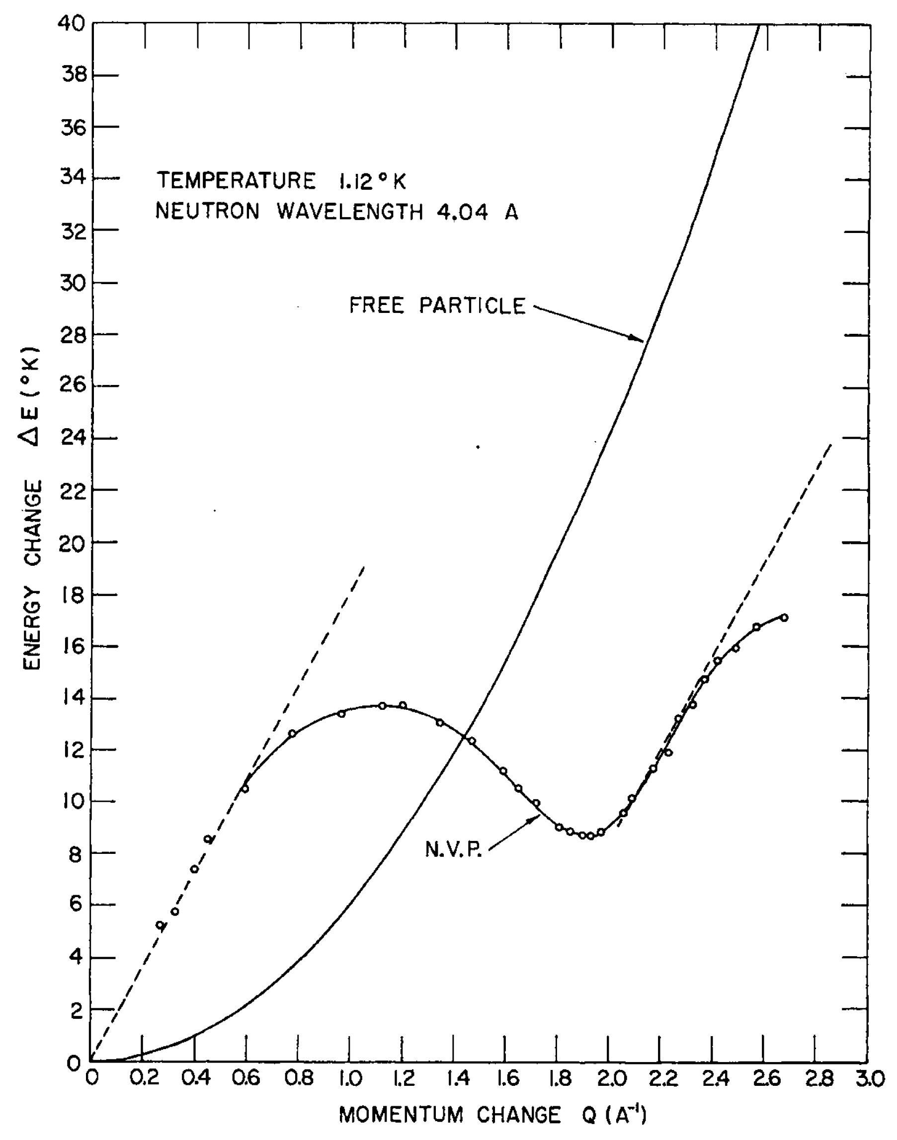
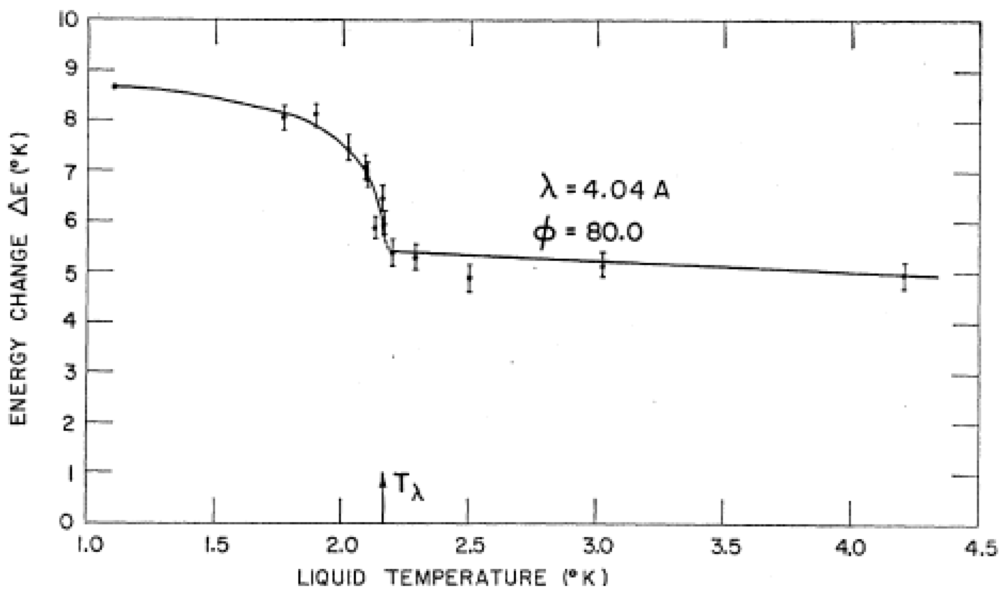
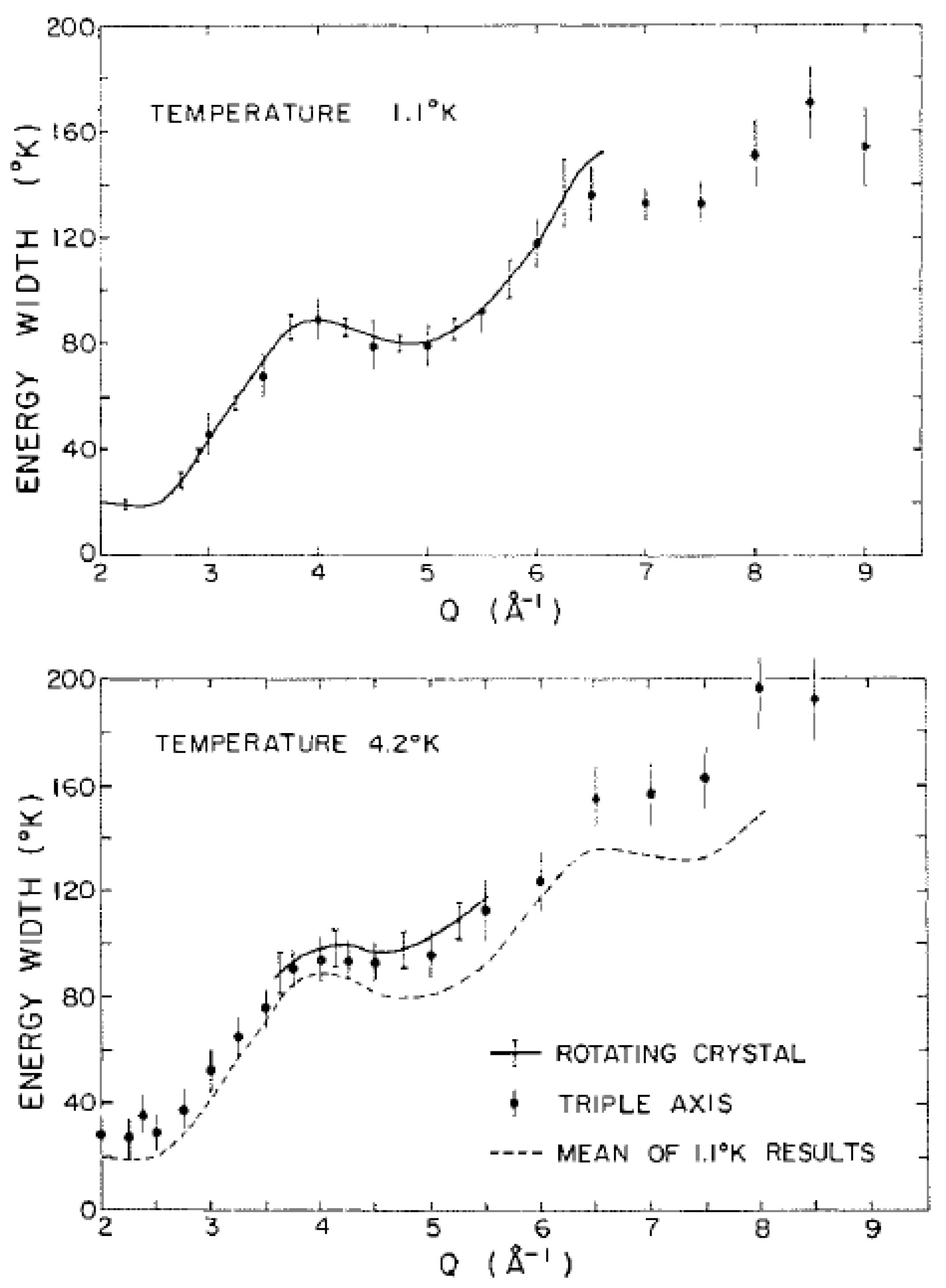
Measurements of the energy–momentum relation in liquid He4 were reported in [40]. Measurements were made at 1.27, 1.57, 2.08, and 4.21 K, below and above the λ-point of 2.2 K, with the rotating crystal spectrometer [41] providing incident neutrons of wavelength 4.14 Å (4.77 meV). A peak in the excitation spectrum was observed at a scattered wavelength of 4.5 Å (4.04 meV) corresponding to an energy transfer of 0.73 meV and wavevector transfer of 1.87 Å−1. Measurements were also made with the Chalk River filter chopper spectrometer [19], and the two sets of measurements were consistent. The measurements of the excitation spectrum, Figure 11, agreed with previous neutron time-of-flight measurements [42,43]. It was noted that as the temperature was raised toward and through the λ-point of 2.2 K, the excitation energies decrease and the widths of the peaks increases. At small momentum transfers, the spectrum tends toward a linear phonon relation and at higher wavevectors follows a form consistent with the Landau [44] roton curve. Under a pressure of 21.4 atmospheres, the scattered energy decreased by about 0.09 meV, which was also in agreement with the prediction of the Landau theory. These experiments marked the beginning of a series of experiments of the inelastic scattering from He4 over a period of 50 years by Henshaw, Woods, Cowley, Svensson, and collaborators.
3.5. Structure of Liquid Neon
The angular distribution of scattering of 1.064 Å neutrons was reported for liquid Ne at 26.0 ± 1.5 K and polycrystalline Ne at 4.2 K in [45]. The measurements were made with an Al monochromator at the crystal spectrometer at the NRX reactor [4] using Söller slits before and after the sample to improve the angular resolution. The temperature of the samples, contained in cylindrical cans, was controlled in a He4 cryostat. Measurements were made from Q = 0.5 to 6.3 Å−1.
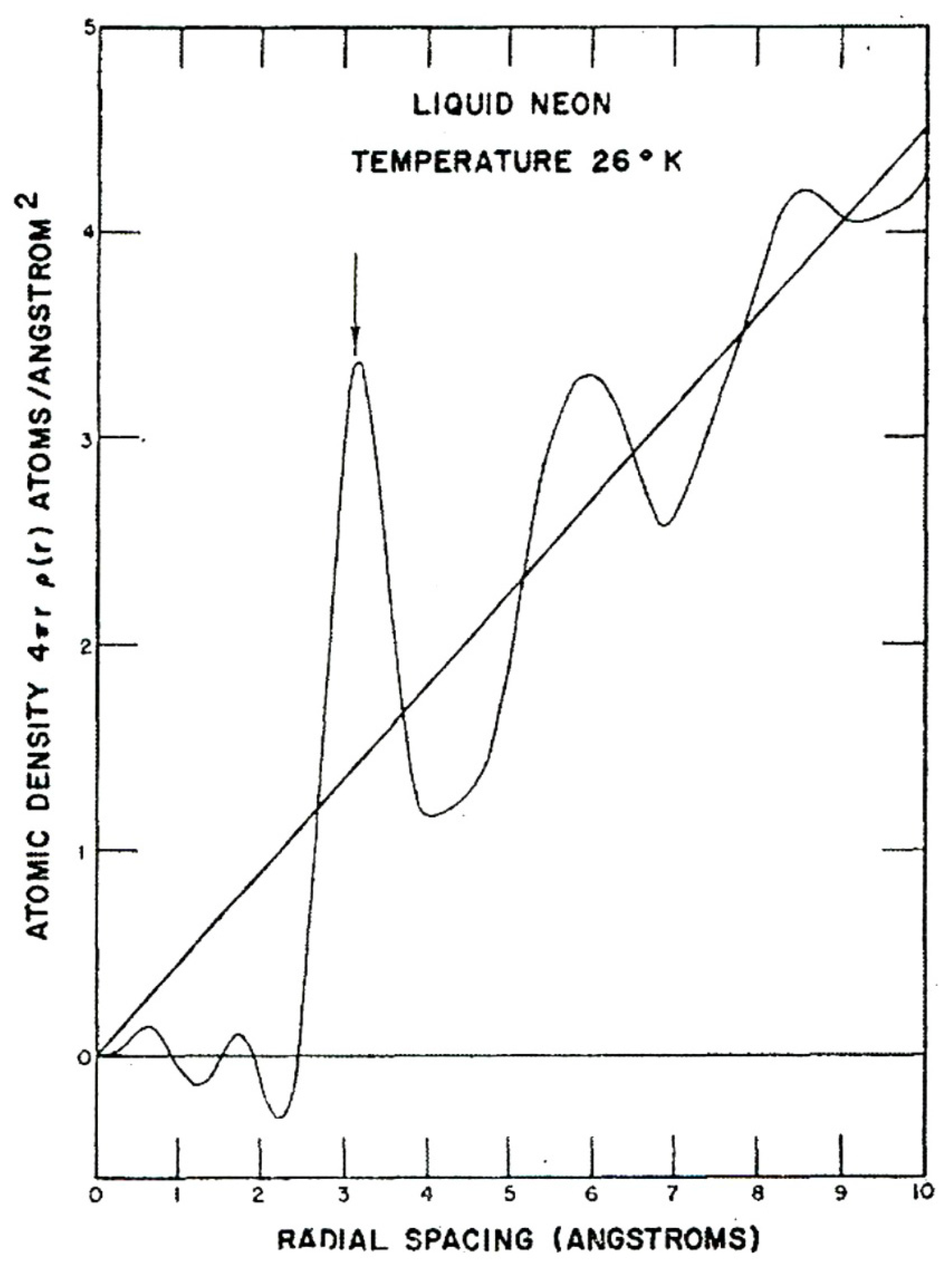
The powder measurements of solid Ne at 4.2 K confirmed the face-centred cubic structure with a lattice parameter of 4.429 Å, the separation of nearest neighbors of 3.132 Å, and a Debye temperature of around 73 K. Similar measurements on solid Ar gave a lattice parameter of 5.256 Å, although the isotopic incoherent scattering of Ar gave a relatively large background underneath the powder peaks. The atomic distribution function 4πrρ(r) in liquid neon is shown in Figure 12. The position of the first peak is close to the separation of nearest neighbors in the solid being about 2.45 Å. The intensity under the first peak yields approximately 8.8 near neighbors around each atom in the liquid. It was concluded that in both liquid Ne and Ar, the form of the effective potential has a broader bowl than that given by a Lennard–Jones potential.
3.6. Dynamics of Water
In the period before 1958, there had been many neutron and X-ray measurements in laboratories around the world, including at Chalk River, of the structure of liquids. Up to this time, there had been few experiments on the dynamics of liquids. The paper on the structural dynamics of water by Brockhouse [46] is remarkable for careful experiments and intuitive physical interpretation in terms of correlation functions. This was especially the case given the small number and the limited energy range of the measurements, which still enabled unambiguous statements to be made about water.
The most widely accepted view of a liquid had been that the structure was semi-stable, that atomic vibrations occur, and that diffusion takes place at fairly wide intervals through activation over thermal barriers somewhat smaller than in a crystalline solid. However, the Maxwell relaxation time is an order of the (speculative) Debye temperature of a liquid, and this should quickly damp out any transverse-type vibrations. Neutron spectrometry clarifies our picture of liquids, since neutrons measure energy changes over a range of wavevectors and are not restricted to Q = 0. The information to be extracted from neutron measurements depends on whether the scattering is coherent or incoherent. The former involves interference between the scattering from different atomic sites and so reveals the liquid structure and its vibrations. The latter does not involve interference and gives information about the movement of one nucleus. Light and heavy water constitute an interesting pair, since the scattering from H2O is 95% incoherent and D2O is about 80% coherent.
The generalized correlation functions were first defined in an important paper by Van Hove [47] and related to the neutron scattering cross-sections. Brockhouse would have met Van Hove at Brookhaven National laboratory, when he spent a year there after the NRX accident and had been introduced to the correlation function approach. In particular, the cross-section factorizes quite generally into a part that depends on the neutron, the parameters that describe its interaction with the nuclei, and a part that depends only on the structure or dynamics of the scattering sample. The correlation functions have simple physical interpretations for monotonic classical systems. The self-correlation function, Gs(r,t), is “the probability that, given an atom at position 0 and time 0, the same atom is at r at a later time t”. The pair correlation function Gp(r,t) is “the probability that, given an atom at position 0 and time 0, any atom is at position r and time t”. The incoherent and coherent partial differential scattering cross-sections per atom are, following Squires [37],
where and are the incident and scattered neutron energies, k and k′ are the incident and scattered wavevectors, and Q = k − k′ is the scattering vector. Note that Squires [37] defines the scattering function S(Q,ω) by
By integrating over the outgoing energy, it can be shown for a classical system that
where is the time in which the neutron travels through the component a distance r along the outgoing direction k′ at its incident velocity. Thus, the validity of the static approximation reduces to the question of whether anything of interest happens to the system in time t0. Quoting from Brockhouse, “Crudely, the neutron experiments are a kind of microscope with a field whose spatial extent is about Å. If the range of neutrons accepted by the counter, within the resolution function, is limited to values between ±ω1, then
and the neutron pattern can be thought of as an average behavior over the time range ”. Since the discussion is of the properties of liquids, the vector character of Q need not be included in the discussion in this case.
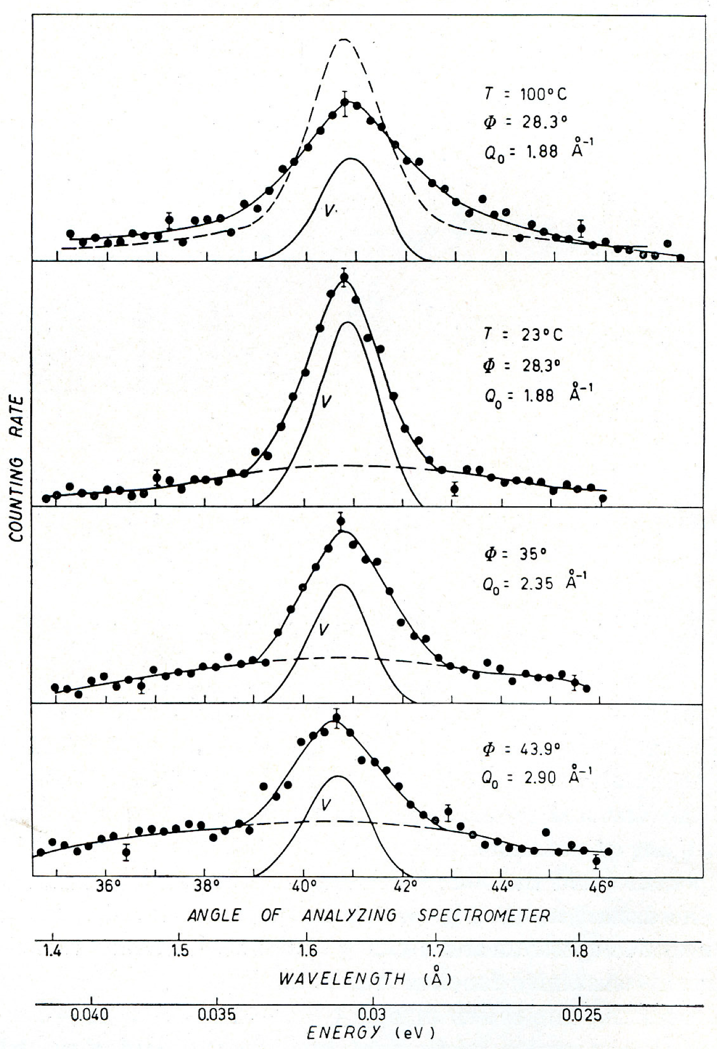
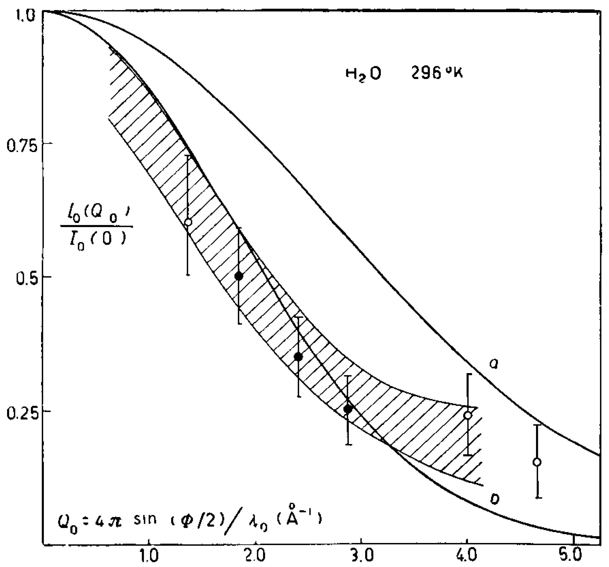
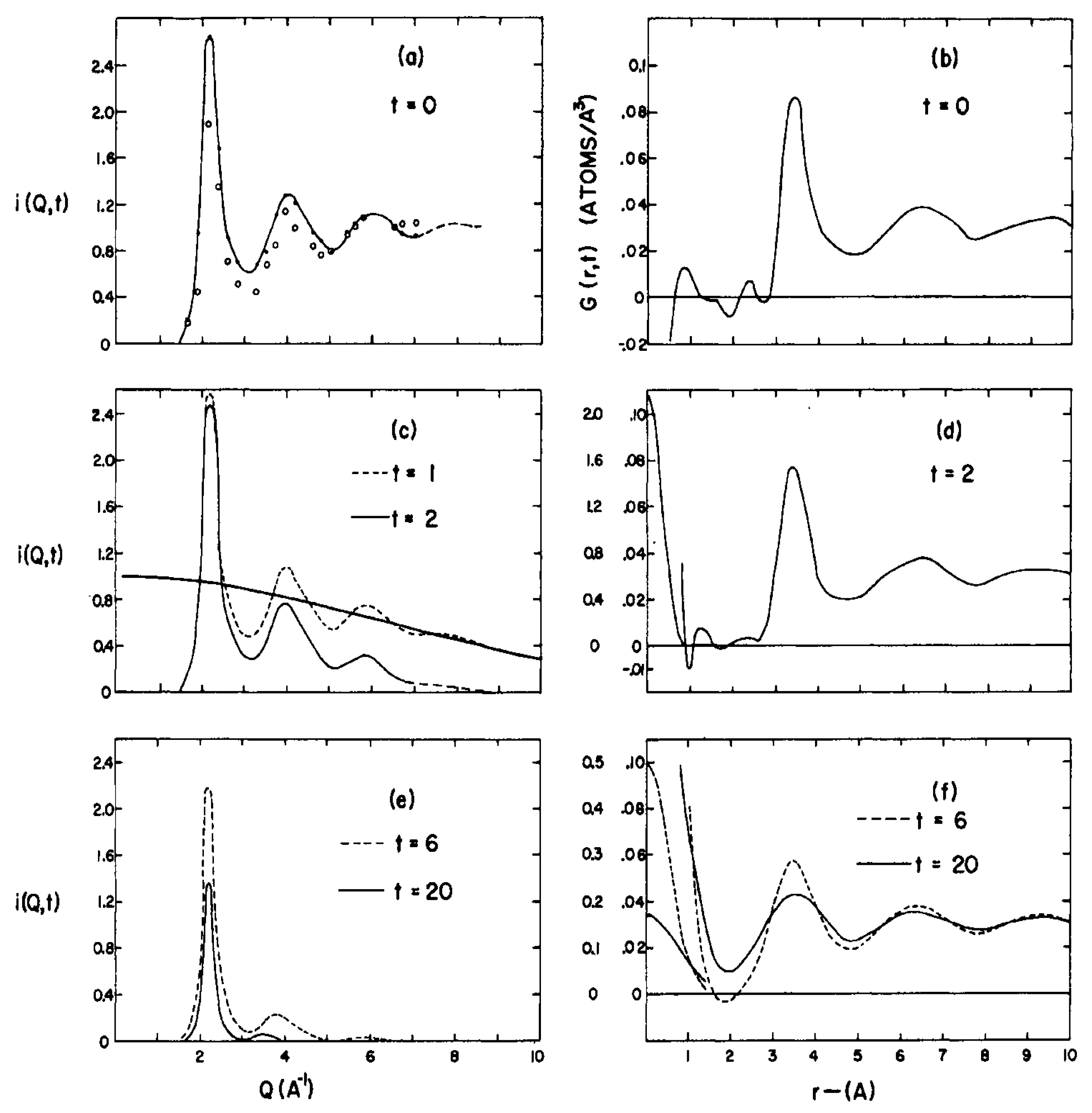
Most of the measurements were made with the crystal spectrometer at the NRX reactor used for phonon measurements with Al (111) planes as monochromator and analyzer in thin samples of water to reduce the multiple scattering. The energy resolution given by the full-width at half maximum of the incoherent scattering from V was about 3 meV. In addition to neutrons of wavelength λ0, about 17% of neutrons of wavelength λ0/2 are present, and these were corrected for. The results for a range of wavevectors near the maximum in the structure factor, 1.88 Å−1 (which cannot be observed in H2O with neutrons because the scattering is primarily incoherent), and beyond are shown in Figure 13, over a limited range of neutron energy gain (11 meV) and loss (6 meV). Brockhouse considered there to be a qualitative separation of energy scales in Figure 13 corresponding to the broad distribution of scattering beyond ±3 meV and a nearly elastic contribution at lower energies. At wavevectors lower than 1.88 Å−1 and greater than 2.9 Å−1, the distinction between the two distributions is less clear, although a fitting process can establish the relative amounts of each. The broad spectrum can be fitted to a calculated spectrum for a monatomic gas of mass (16 + 2 = 18) at all wavevectors, and at 8 Å−1, all the scattering can be attributed to a gas of mass 18. For H2O, the quasielastic scattering has a maximum at Q = 0 and has diminished to zero at 5 Å−1, as shown in Figure 14, and it follows a Debye–Waller like form with about 0.4 Å. The width of this distribution increases with Q and the different kinds of diffusive motion, jump-type and continuous, which have different Q dependences. Brockhouse concluded that both contribute to this width. The fact that the broad inelastic contribution could be simulated by a gas of mass 18 indicated that the scattering observed originated from scattering by the whole molecule. Measurements with the filter difference spectrometer [19] in neutron energy gain at 300 K showed the presence of a peak in the scattering around 60 meV, which is in the same energy range, 30–110 meV, as the band of hindered rotations observed in Raman scattering by Cross et al. [48].
Measurements were made on D2O at 1.88 and 2.33 Å−1, at which wavevectors there had been a clear separation between the inelastic and quasielastic contributions in H2O. The inelastic contribution is far smaller for D2O because of the ratio of the scattering cross-sections, 19/168. At a resolution of 3 meV, it was difficult to separate the two contributions. The broad part appeared wider at the higher wavevectors but is still narrower than expected on the basis of continuous diffusion. However, the correlation function that enters does include effects from the oxygen atoms, and so the scattering would be expected to be different.
In the general discussion, Brockhouse pulled together the neutron results as well as the macroscopic measurements to give an intuitive picture of the dynamics of water. He considered that the neutron results can be interpreted by assuming that a thermal cloud is formed, which can be approximated roughly by a Gaussian self-correlation function of root mean square radius of about 1 Å, although it is more diffuse than a Gaussian. After formation, the cloud expands slowly by small motions, but this expansion does not account for the whole of the measured diffusion constant, and large diffusion jumps must be invoked to account for the difference. The fact that measurements of the high frequency dielectric constant can be fitted by a single relaxation time suggests that both the diffusive motions and the reorientation of the molecules occur simultaneously at a time of breakdown of the local structure. Clarifying the physics involved required measurements of resolution around 0.1 meV.
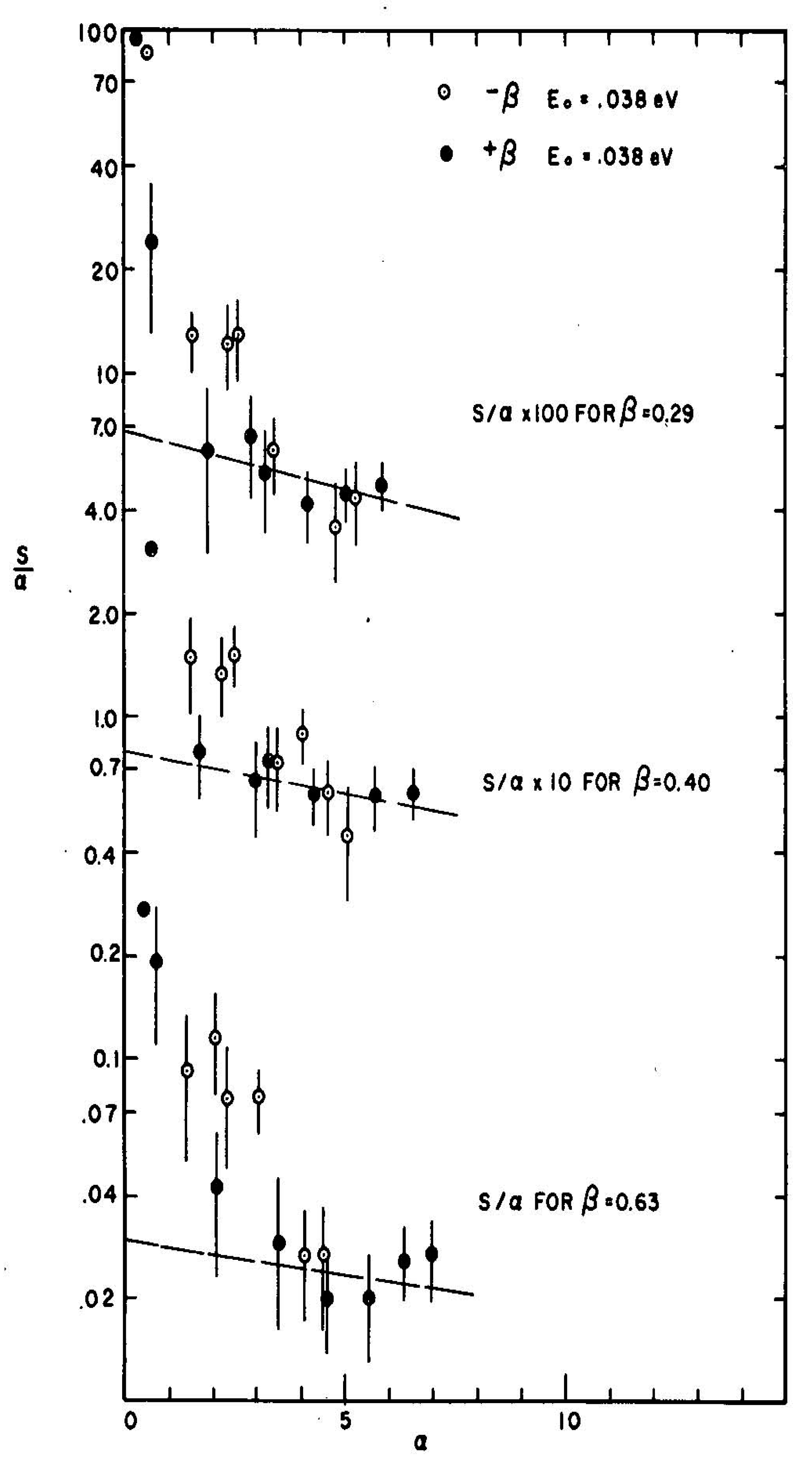
The high-resolution measurements to investigate the diffusion behavior were subsequently reported by Brockhouse [49] and Sakamoto et al. [50] for water at 25 and 75 C. The measurements were made with the Chalk River rotating crystal spectrometer [39] with an incident energy of E0 = 4.964 meV and an energy resolution of 0.2 meV. The data were corrected for fast neutron background, air scattering, second-order wavelength contamination of the incident beam, counter efficiency, and multiple scattering. Twenty measurements at different scattering angles were used to create a grid of S(Q,ω) in steps of 0.2 Å−1 and 0.05 meV, as seen in Figure 15, which was then Fourier transformed to obtain the self-correlation function Gs(r,t). Only diffusive broadening of the quasi-elastic peak was observed over the whole range of ω (50 meV) and Q (2.0 Å−1). The energy width, W, of the diffusive peak, corrected for resolution, followed the relation
where D is the coefficient of self-diffusion at small Q but falls below at larger Q. The mean square displacement <r2> for water derived from the data followed the diffusion law <r2> = 6Dt at times greater than 6 × 10⁻¹² s.
3.7. Magnetic Structure of Chromium Oxide
The antiferromagnetic structure of powder Cr2O3 (TN = 318 K) was determined by Brockhouse in 1953 [51]. Measurements were made at 80 and 295 K with 1.303 Å neutrons from a crystal spectrometer, and the reflections were indexed on the basis of the rhombohedral unit cell. Strong increases in the intensities of the {110}, {211}, and {200} reflections at 80 K were ascribed to magnetic Bragg scattering. Four Cr ions lie on the <111> diagonal of the unit cell, and three possible antiferromagnetic structures may occur, namely ↑↓↑↓, ↑↑↓↓, and ↑↓↓↑. Values of the magnetic structure factor were calculated and compared with experiment, and it was concluded that the ↑↓↑↓ arrangement was consistent with the strong intensity increases of the {110}, {211}, and {200} reflections and the absence of a magnetic contribution to the {210} reflection. With a polycrystalline sample, it was not possible to assign the crystallographic orientation of the Cr moments.
3.8. First Crystallographic Texture Measurements with Neutrons
In connection with the publication of his doctoral thesis experiments on the initial magnetization of nickel [52], Brockhouse made the first neutron measurements of crystallographic texture with a crystal spectrometer. The experiments were carried out on annealed Ni wire for which the (111) plane normals are strongly aligned and the (002) normals more weakly aligned with the wire axis corresponding to a fiber texture. He recognized the advantages that neutrons have in averaging over a large volume of materials and many crystallites even if these are large, the high penetration of thermal neutrons, as well as the insensitivity to surface treatment compared with X-rays. Ni wires were cut into short lengths and secured to Al foils so as to fill the area of the neutron beam in transmission geometry. No corrections were needed for geometry or for absorption. Brockhouse [6] also referred to neutron diffraction tests of preferred orientation in Ni wires and Al foils. A texture goniometer was constructed, and measurements of diffracted neutron intensity as a function of the angle of the sample were described in Chalk River progress reports in the fall of 1952. Studies of rolled Al foils showed that the orientation of crystallites was largely determined by the rolling direction of the foil. Brockhouse realized that the intensities of some Debye–Scherrer diffraction peaks could be reduced to near zero by proper setting of the rolling direction, and that such oriented foils would be useful for the windows of cassettes for powder diffraction. Texture measurements were also made on a uranium sphere cut from an NRX fuel rod, and the results augmented previous X-ray measurements. A reference was also made in [1] to neutron texture measurements on uranium, although the work was never published in the open literature.
3.9. Inelastic Paramagnetic Scattering
The first report of measurements of inelastic paramagnetic scattering of neutrons was described in a paper entitled “Energy distribution of neutrons scattered by paramagnetic materials” in 1955 [53]. Paramagnetic scattering is an incoherent process originating in the scattering of the neutron magnetic moment by the disordered electronic magnetic moments above the magnetic ordering temperature. Integrated over energy, paramagnetic scattering contributes to the differential cross-section dσ/dΩ along with the nuclear incoherent scattering, multiple phonon scattering, etc. It is expected to follow a magnetic form factor as a function of Q. Van Vleck had shown for a molecular field model that the root-mean-square energy change could be written
where Z is the number of magnetic neighbors, S is the spin on the atom, and θCW is the Curie–Weiss temperature determined by fitting the paramagnetic susceptibility to the Curie–Weiss Law
Van Vleck had also calculated the moments of the scattering and suggested that the energy distribution would be close to Gaussian.
The measurements were made on MnSO4 (Mn2+) and Mn2O3 (Mn3+) with a fixed incident wavelength of 1.3 Å reflected from an Al mosaic monochromating crystal recently grown by Henshaw at Chalk River. The measurements were carried out at the NRX reactor. The energy analysis was carried out by stepping the scattered neutron wavelength through 1.3 Å by varying the angle of scattering from a second Al “analyzer” crystal. The intensity at zero energy transfer, corrected for ambient background, nuclear incoherent and multiple scattering, was expressed as a cross-section by calibration with the known incoherent cross-section of vanadium and shown to follow a 3d form factor with values in the forward direction of S = 5/2 and 2, respectively. That is, the Q-dependence of the scattering was shown to be magnetic and originating in the scattering from the known magnetic moments. Both materials showed energy distributions that were consistent with a Gaussian form. MnSO4 showed an energy distribution no wider than the instrumental resolution, but Mn2O3 showed a width greater than the instrumental resolution. The results were consistent with the low Curie–Weiss temperature, θCW = −24 K and low Néel temperature, TN = 14 K, of MnSO4 and the larger θCW = −176 K and TN = 80 K of Mn2O3.
3.10. Spin Waves in Magnetite
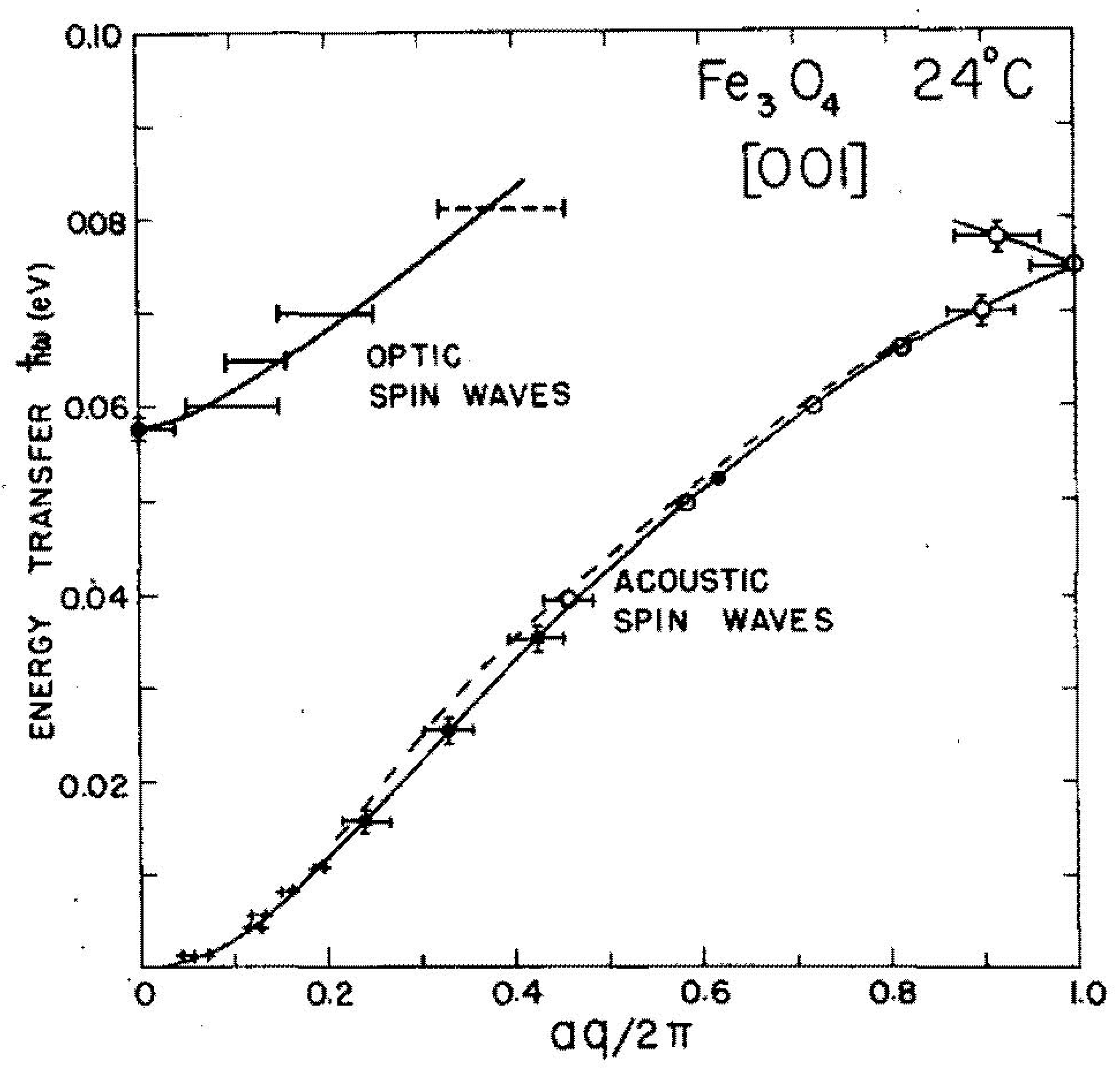
The first measurements of magnetic excitations in an ordered magnetic material, magnetite, Fe3O4, were reported by Brockhouse in 1957 [54]. To put the paper in context, it was generally thought that the excitations out of the fully ordered magnetic state were wavelike by analogy with the vibrations of the crystal lattice. However, only integrations over the dispersion relations contribute to thermodynamic measurements such as magnetization and low-temperature specific heat. The theory of neutron scattering by spin waves had been worked in the previous decade (here, theory was ahead of experiments), and it was shown the neutron-spin-wave system should obey the same conservation laws in momentum and energy as the lattice vibrations, namely Equations (2) and (3).
Unambiguous measurements can only be made on single crystals, and the existence of large natural crystals prompted the experiment. However, this brought a number of new problems, since natural crystals are rarely pure, and this sample had 10% of the iron sites replaced by other ions. The magnetic unit cell of magnetite contains 8 Fe3+ (S = 5/2) ions on A sites and 8 Fe3+ and 8 Fe2+ (S = 2) ions on B sites. The ions on A sites are antiparallel to those on B sites, leading to ferrimagnetism. At temperatures below 119 °K, the Verwey transition, the Fe3+ and Fe2+ are ordered on the B sites. There are six interpenetrating magnetic sublattices, and therefore, there is one “acoustic” mode that goes to zero energy at q = 0 and five “optic” branches. The question arose: “Could the magnetic excitations be seen above the other contributions to the scattering, especially since Fe and O are strong coherent scatterers and give rise to intense lattice vibrations and there is a large diffuse contribution from the impurity content of the crystal?” Brockhouse estimated that the total incoherent scattering, both nuclear and magnetic, was between 5 and 8 bn per Fe3O4 formula unit. Multiple scattering, in this case neutron inelastic scattering preceding or following Bragg scattering in the crystal, will augment the incoherent scattering. With characteristic thoroughness, measurements of the intensity integrated over energy in the form of a differential scattering cross-section, dσ/dΩ, calibrated with a standard V sample, were made and shown to be consistent with the estimates of intensity. In the experiment, measurements were made around the (111) reflection, which is primarily (97%) magnetic. Since the measurements were made at a relatively small angle, 8.1°, fast neutrons coming down the main beam would have been a problem, and tight collimation was used. Close to, but not at the (111) peak, dσ/dΩ, becomes very intense, as had been seen previously [55], and it was the investigation of this intensity that yielded the spin-wave behavior under energy analysis.
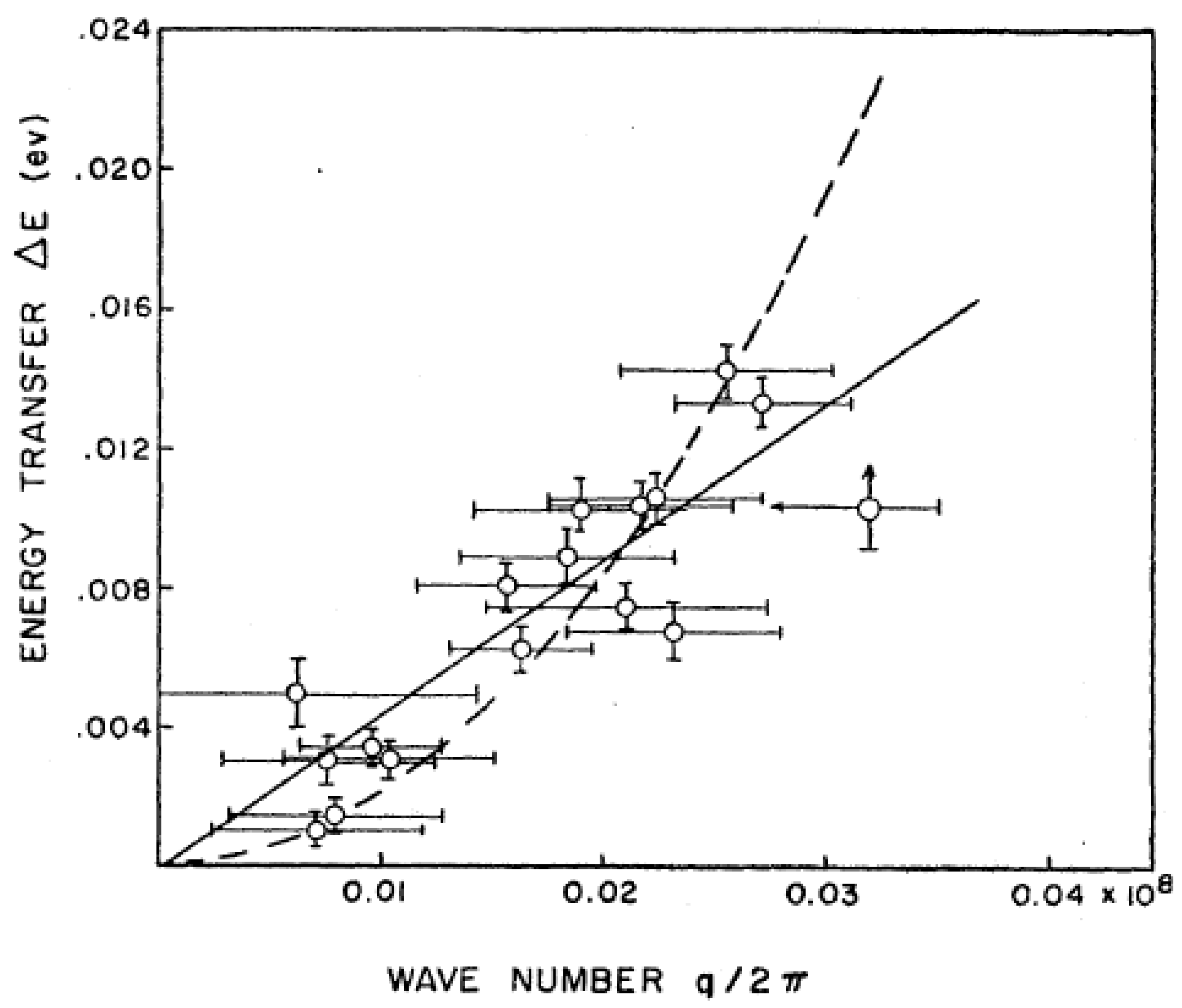
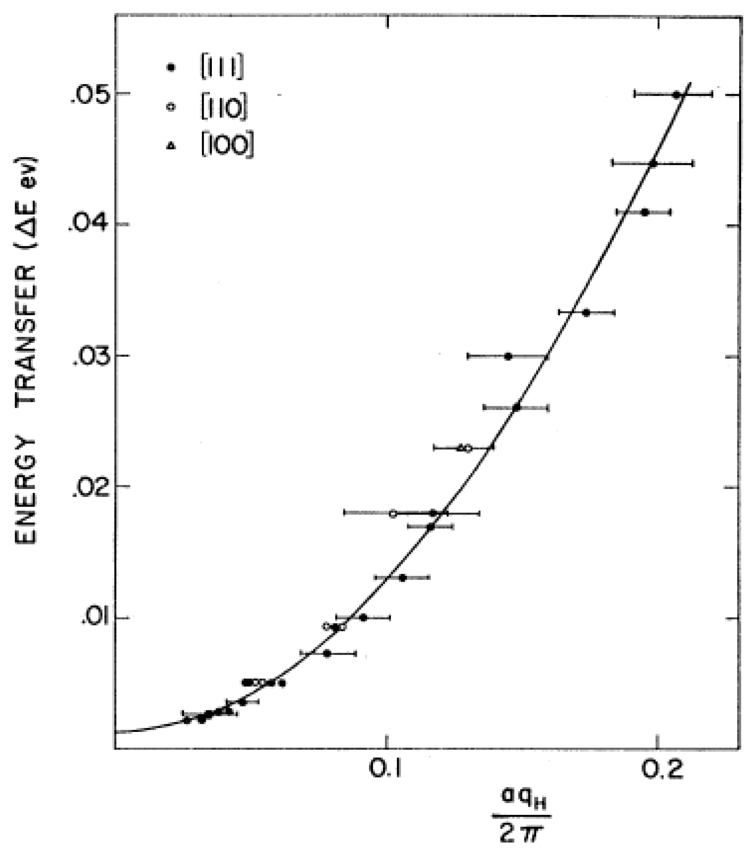
The spin-wave dispersion relation is shown in Figure 16 over a frequency range of 4 THz (16 meV) and wavevector range up to 0.04 Å−1. It was not possible to decide on the basis of the initial experiments whether the dispersion relation was linear or quadratic because of the scatter. However, the line through the data certainly did not correspond to the velocity of sound in magnetite and therefore was not a phonon dispersion relation seen through the magnetic cross-section (magnetovibrational scattering). For a linear dispersion relation, the dominant exchange interaction, JAB, would be 122 K (or 10.5 meV, 2.5 THz), while for a quadratic dispersion relation, JAB, it was 23.2 K (or 2.0 meV, 0.48 THz). On the basis of the latter number, the calculated Curie temperature in a molecular field model would be 1050 K, which is not too far from the actual value of 850 K. On this physical basis, it was concluded that a quadratic dispersion relation was more reasonable.
The final confirmation that the observed excitations were in fact spin waves came from a comparison between the measured cross-sections and values derived theoretically by Elliot and Lowde [56]. It was guessed by Brockhouse that near q = 0, the relative phases of the spin deviations would be the same as the static magnetic moments. On this basis, he guessed the structure factors and found them to agree within reason with the measurements of d2σ/dΩdE. Further work was promised on the temperature and field dependence of the intensities, which are unambiguous for magnetic materials.
In a paper written shortly afterwards [57], Brockhouse showed that the intensity variation of the spin waves in an applied magnetic field was consistent with the cross-section for magnetic excitations. The cross-section for transverse spin waves is proportional to (, where and are unit vectors along the scattering vector and the magnetic moment direction is along the <111> direction for magnetite. There are eight such domains in a zero magnetic field. The spin-wave intensity was measured near the (111) reciprocal lattice point in a zero field where = 1/3 and in a field of 3.5 kG aligned to saturation along the [111] direction where = 1. The field-on to field-off ratio is expected to be 1.5 and was observed to be 1.42 ± 0.05. The final sentence of the paper states that: “The results described herein complete the identification of the excitations previously observed, as spin waves of the usual description.”
4. Post Development of the Triple-Axis Crystal Spectrometer and Constant-Q, 1957–1965
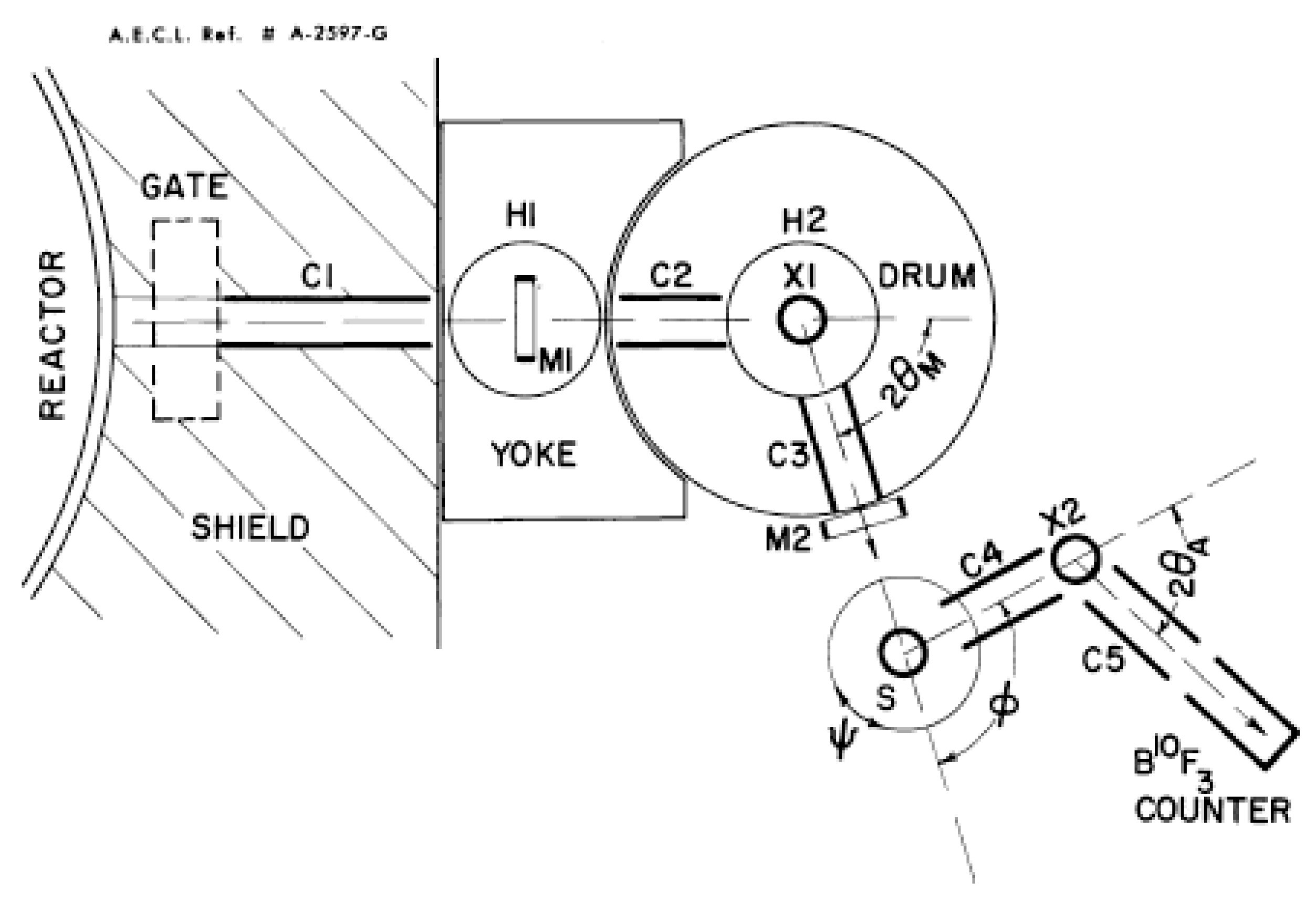
1957 was an important year for neutron research in Canada, since the National Research Universal, NRU, reactor started in November with a power of 200 MW and thermal neutron flux of 3 × 10¹⁴ neutrons·cm−2 s−1, which is about a factor of 10 higher than NRX. A newly designed triple-axis spectrometer was being built at the NRU reactor, and immediately following the restart of the reactor after the NRU accident in the fall of 1958, it was rapidly deployed. In describing the instrument at the Conference on Neutron Scattering in Solids and Liquids in 1960 in Vienna, [41], Brockhouse said, “The C5 triple-axis crystal spectrometer at the C face of the NRU reactor was designed to be as flexible and generally useful as possible, allowing a wide range of energies, E and E′, and scattering angles, Φ, and crystal angles, Ψ. The resolution was readily changeable.” The neutron flux of all wavelengths at the source, which was 6 m from the spectrometer, was 2 × 10¹⁴ neutrons·cm−2 s−1.
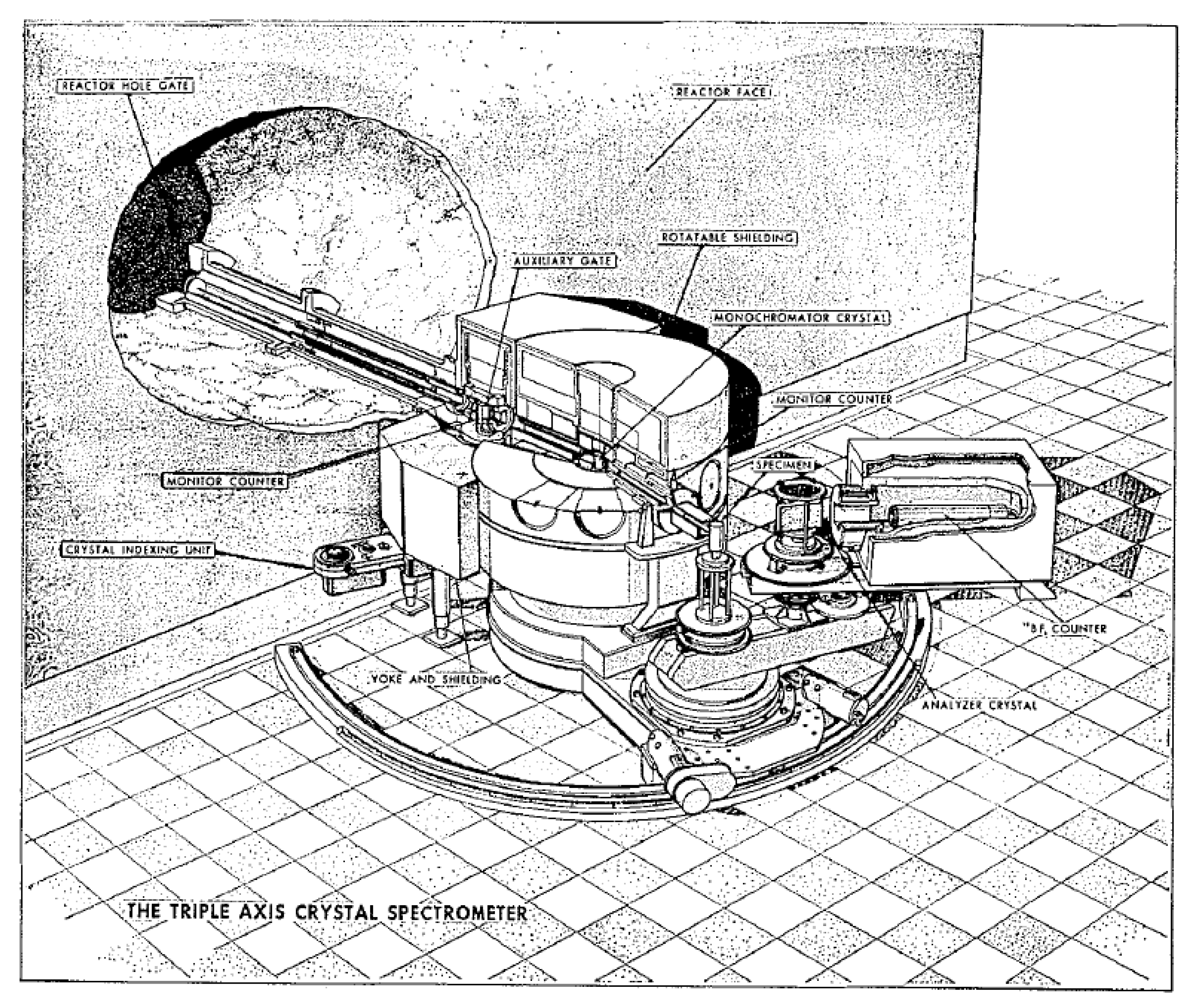
A schematic of C5 is shown in Figure 17 with a cutaway sketch in Figure 18 of its installation at the C-face of the NRU reactor. The monochromator assembly comprises a heavy shielded drum, collimators, a monochromator crystal, X1, and a large moving platform with an accurate vernier scale, which carries the sample table, analyzer, and counter. Arguably, this is the most crucial part of the instrument, since it has to provide accurately moving parts and provide good shielding against the fast neutrons and gamma rays emerging from the beam tube. It was designed by W. McAlpin, who had worked on ship structures on the River Clyde in the UK during the war. The monochromator angle θM followed the turning of the drum, the monochromator scattering angle, 2θM, at half speed.
The positional spectrometer was basically the unit described by Hurst et al. in [4]. It consisted of a heavy arm whose angular position, Φ, is the sample scattering angle and the crystal table, Ψ. Both scales were read on accurate Vernier scales.
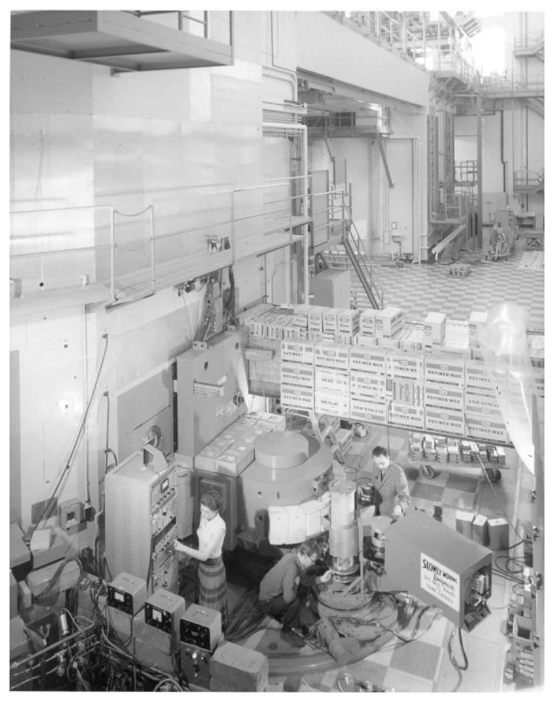
The analyzer is mounted on the arm of the Φ table. The analyzer crystal angle θA is connected to 2θA by a half-angling mechanism, and both were provided with accurate angular scales. The BF3 (96% B10) counter was 6.2 cm in diameter and 25 cm long and was made at Chalk River. A paper-tape control system was used, and the tape contained angular increments in 2θM, Φ, Ψ, 2θA prepared on the Chalk River mainframe computer corresponding to constant-Q or constant-υ scans. The monochromator and analyzer crystals were mounted on permanently aligned mounts and cut from single-crystal ingots of Al with the [] direction vertical allowing access to the (111), (002), (220), (113), and (331) monochromator planes. Adjustable collimators were made of Cd-coated steel strips which slid into slots in the collimator boxes. Collimations around ½ to 1° were used at collimators C3 and C4 to define the beam directions and were relaxed at collimator C5. The collimation before the monochromator, C1, C2 is defined by the beam apertures and the distance to the source, and it is of order 1°. A photograph of the spectrometer taken in about 1965 is shown in Figure 19.
In concluding his presentation at the IAEA conference in Vienna [41], Brockhouse commented, “We now use almost exclusively the procedure in which the outgoing energy, E′, is fixed and the incoming energy, E, varied. The monochromatic beam is monitored by a fission counter whose response is almost 1/v, and counting is done for a preset number of monitor counts. This procedure eliminates the analyzer reflectivity with respect to wavelength and takes account of the k′/k factor in the inelastic cross-section so that the counts are almost equal to S(Q, ω) directly”.
In 1958, A.D.B. Woods was hired by Brockhouse, who was embarking on studies of phonons in semiconductors, metals, and alkali halides. Up to this point, measurements of dispersion relations in high-symmetry directions had to be made by an iterative process, since there was no guarantee that measurements with a fixed incident energy, E, and varying E′ to measure the scattered peak would yield a phonon wave vector on a symmetry direction. Dave Woods, in a private communication, described the discovery of the constant-Q method in this way:
“I remember the Monday morning that Bert came in and announced his idea of the constant-Q method of observing phonons. A few weeks earlier, R.G. Stedman from Sweden had arrived at Chalk River to work for a year in P.A. Egelstaff’s United Kingdom Atomic Energy group on scattering from neutron moderators. Dr. Stedman had explained to us attempts made in Sweden to observe phonons in NaCl on the initial steep branch of the dispersion relation by moving at constant energy transfer across the curve. Bert brilliantly clued into this and realized that if you could control the angle of scattering and the sample crystal orientation along with the energy transfer, you could do a scan without changing the momentum transfer, hence constant-Q”. The awkward Jacobian defined in Equation (13) becomes unity in the constant-Q method.
4.1. Lattice Dynamics of Crystals
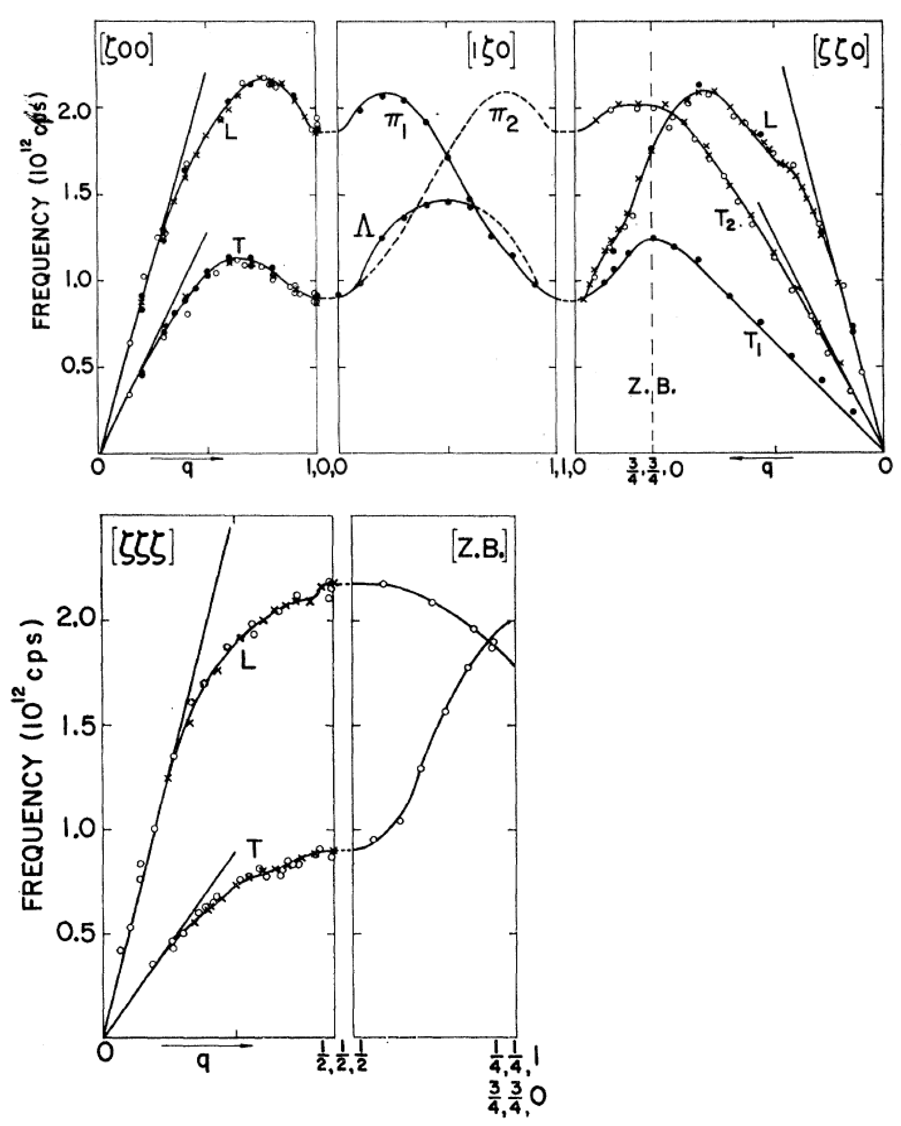
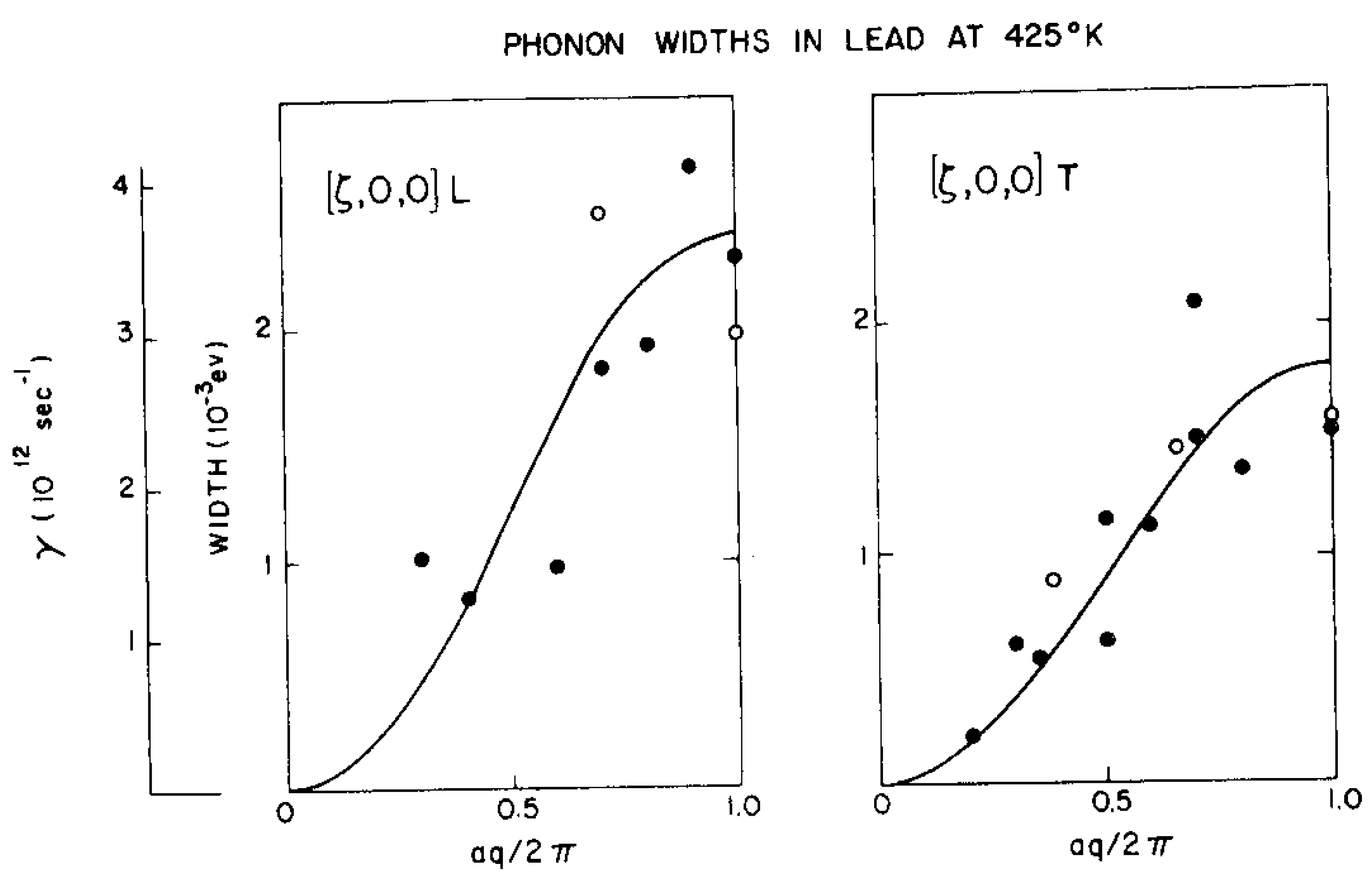
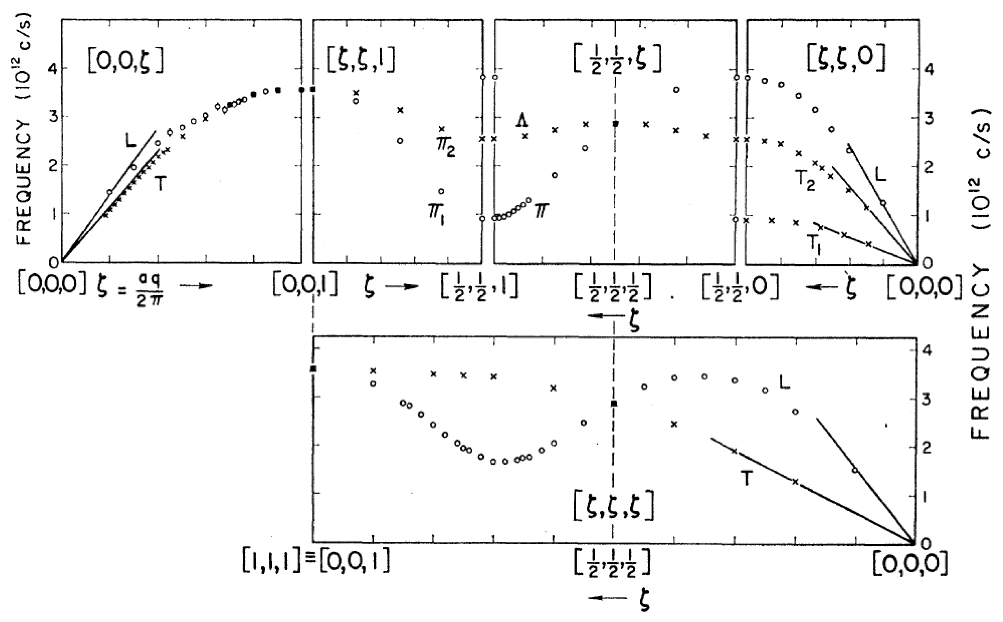
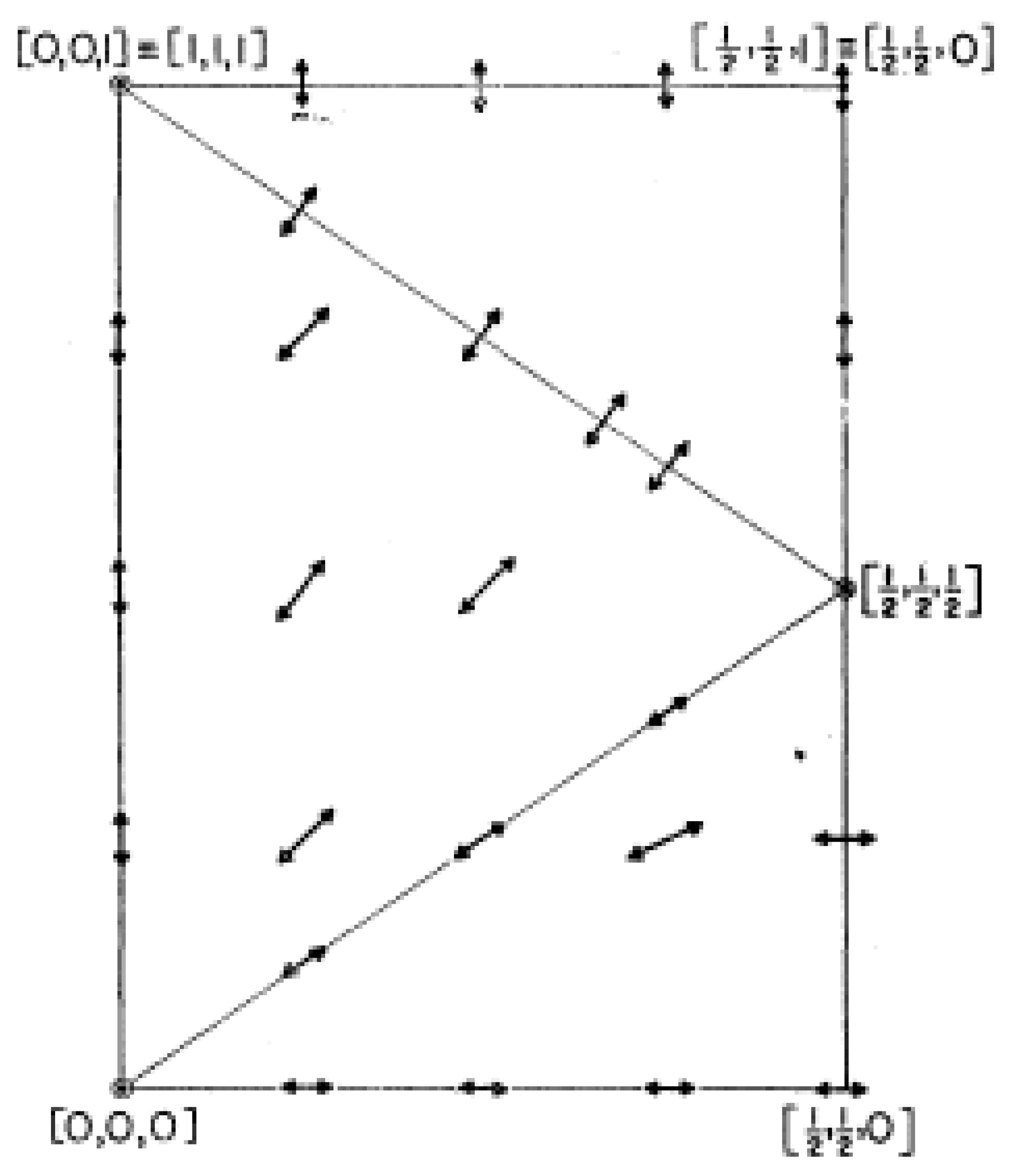
4.1.1. Lattice Dynamics of Lead
The lattice dynamics of solid lead between 110 and 425 K were thoroughly discussed in references [59,60,61]. Lead was chosen due to the availability of large single crystals, the likelihood that only the outer four valence electrons would determine the force constants, it being a superconductor with a high transition temperature, and the electron–phonon interaction probably being strong. While the early measurements were made with the rotating crystal spectrometer at the NRX reactor, the majority of measurements were made with the triple-axis crystal spectrometer at the NRU reactor employing Al crystals for monochromator and analyzer, firstly with the “conventional”, i.e., constant k, method and then with the constant-Q method. The energy versus wavevector dispersion relation for Pb at 100 K is shown in Figure 20; it is far from being a simple sine curve and clearly displays higher-order harmonics. The neutron groups at higher temperatures are broadened but superposed on a strong sloping background, which was ascribed to two subsequent single phonon scattering events in the large crystal as well as multiphonon scattering. After absorption corrections and taking out the population factors and assuming that the cross-section is independent of temperature, the full-widths at half-maximum of the peaks at 425 K are shown in Figure 21.
The width data were interpreted in terms of a phenomenological extension of the Born–von Kármán theory of lattice dynamics to include, as well as restoring forces depending linearly on the relative separation of the ions, dissipative forces depending linearly on the relative velocity of the ions. The equation of motion for the lth atom for a particular mode in a high symmetry direction is
where ul is the displacement and Φ and Γ are the restoring and dissipative force constants between the l and l′ atoms. We assume the solution to be a damped wave of form
where γ is a rate constant for the decay of the wave. Then, the equations of motion become, using interplanar force constants,
and
Foreman and Lomer [25] had earlier suggested that a simple way of interpreting the evident higher harmonic terms present in Pb, to estimate the range of the forces involved from the dispersion relation, was to use interplanar force constants, as suggested in Equation (10). Brockhouse et al. followed this approach and showed that interplanar force constants out to n = 4 or possibly 5 (corresponding to eight shells of neighbours) were sufficient to describe the data at 100 K. As a function of temperature, the Φn decreases faster as n increases. Brockhouse et al. postulated that damped phonons have an energy dependence that follows a Lorentzian form
with a FWHM of ħγ. The variation of 1/γ with q appears to follow a sine variation, as Figure 21 shows, and 1/γ may be interpreted as the lifetime of the phonon. Its value at the [00ζ] zone boundary is about 30% of the phonon frequency, showing that the lifetime is only about 50% of the period of the wave. The origin of the widths, whether due to electron–phonon or phonon–phonon coupling, remained unknown at that time.
Brockhouse et al. [58,59] had noted the sharp changes in curvature in the dispersion relation of lead and had speculated that these were Kohn anomalies where the phonon can excite an electron across the Fermi surface. High-resolution measurement at the same phonon wavevector, q, around different reciprocal lattice vectors, τ, proved that this was the case and constituted the first such direct observation of the interaction between phonons and electrons [61]. The experiments were carried out at the NRU reactor with the constant-Q technique with a relative error from point to point of ±0.05 THz. For a spherical Fermi surface, the positions of the anomalies occur where the sphere cuts the wavevector, q, are given by
Spherical Fermi surfaces in reciprocal space may be drawn centered on several τ, for example, (000), which gives a circle in the () plane, or (200), which gives an arc in the () plane. The most marked discontinuity is at , and this position is in fair agreement with the dimension of the Fermi surface, assuming it to be spherical or as determined by de Haas–van Alphen measurements. The anomaly at is also expected to be strong but may have contributions from two different pieces of the Fermi surface. Actual discontinuities such as the Kohn anomalies in Pb underline the long-range nature of the electronic origin of the forces and are not sensibly amenable to the interplanar approach.
4.1.2. Lattice Dynamics of Sodium and Potassium
Following immediately on the paper describing the lattice vibrations in lead was a study of the phonons in the body-centered cubic metal, sodium [62,63]. With one valence electron outside a closed shell, sodium is expected to have a simple electronic structure, and therefore, there is a good possibility of understanding the lattice dynamics at a fundamental level. The dispersion relations were interpreted within Born–von Kármán theory in terms of force constants extending out to 5th nearest neighbors. The frequencies of the measured normal modes for the [ζ00] direction were written in terms of three interplanar force constants [25] as in Equation (10), where φn is a linear combination of the atomic force constants α1, β1, α2, etc. The contributions from the five nearest neighbors are given explicitly in Tables 1 and 5 of ref. [63]. Typically, the ratio of φ3 to φ1 is about five to ten times smaller for Na than for Pb. The single crystal of Na, having a length and diameter of 4.5 cm, was encased in a thin-walled Al can to prevent oxidation. Measurements were made on the C5 triple axis crystal spectrometer at the NRU reactor by the constant-Q method. The majority of measurements were made at 90 K, and measurements at 215 and 296 K showed that the frequencies decreased by a few percentage points, and the phonon widths increased as the temperature approached the melting temperature of 370.6 K. The dispersion relation for Na at 90 K is shown in Figure 22. The Fourier analysis showed that while three terms, corresponding to five shells of neighbors, gave quite a good fit, a more precise fit required n = 5, corresponding to eight shells of neighbors, but with values which were only of order 1% of φ1. Na is non-superconducting, unlike Pb, and the electron–phonon interaction is very small. Considerable effort was spent to see whether there were any Kohn anomalies in Na where the Fermi surface is nearly spherical and well known. There were no discontinuities in the dispersion relation to within 1% in the locations where the free-electron Fermi surface cuts the dispersion relation in wavevector.
The polarization vectors within the () plane for the LA and TA modes are initially unknown (although in high-symmetry directions, they are readily deduced from symmetry considerations), but they may be obtained from the intensities of the phonon groups, as shown in ref. [64]. For a constant-Q scan, the cross-section and hence the integrated intensity is given by
The usual factor in the cross-section is canceled by the use of a monitor fission counter in the monochromatic beam with an inverse velocity response, in which Nj is the temperature factor and gj is the structure factor.
Here, bl is the scattering length for the lth atom in the unit cell, and is the polarization vector for the lth atom in the jth mode. The ratio of the integrated intensities of the neutron groups for the two modes, one longitudinal and one transverse, propagating in the plane is, for neutron energy loss, for monatomic Na
If β is the angle between the wavevector transfer, Q, and the [001] axis and α is the angle between and the [001] axis, then
from which α may be obtained. The main source of uncertainty in the case of Na is the high incoherent inelastic background underneath the phonon peaks. The polarization vector of the highest mode in the ( plane is shown in Figure 23, where the non-intuitive results lie in the interior of the reduced Brillouin zone for Na. Similar measurements were made for Ge with six phonon branches to test further how accurately structure factors could be obtained from phonon intensities. For the [00ζ] L branch, which should exhibit the same structure factor at all points, the root-mean square deviation from the mean was ±7%. For the (¼¼¼) LA mode measured at four distinct points in reciprocal space, the measured average structure factor was 3.7 ± 0.1, the calculated value was 3.65, and similar reasonable agreement was found for the [ζζζ] TA mode.
Measurement and analysis of the lattice dynamics of K follow logically on from the experiments on Na, although these were reported much later in 1966 [65]. K was chosen since the incoherent scattering is relatively much less than Na, there was no Martensitic transformation in potassium, and the experiment could be done at 9 K, where there was less likelihood of anharmonicity. The dispersion relations in the () plane are shown in Figure 24 and map onto those of Na with a single scaling factor of 1.65. The data were fitted, as in the case of Na, with a Born–von Kármán model with axially symmetric force constants up to 5th nearest neighbors, and the fits are shown in Figure 24 as solid curves. From this fit, g(υ) was calculated and hence the temperature dependence of the Debye temperature, θD, which was in substantial agreement with the experiment.
In the Born–von Kármán theory [23], the frequencies and polarization vectors are related to the interatomic force constants, as in Equations (5) and (6), by
where Uα, specifying the polarization of the mode, obeys certain orthogonality relations and Φαβ(0,l) are the atomic force constants following the notation of ref. [65]. The equations are non-linear, and it is not possible to solve uniquely at a general point in the Brillouin zone unless both the frequency squared and the polarization vector are known. Since measurements are typically made in high-symmetry directions, such as [ζζζ], in general, the force constants derived from these measurements alone are not unique. This effect was also noted in [66] for Ni and also for Si by Dolling [30], where there are sometimes ambiguities in the fits such as non-physical parameters.
Following Cochran’s work on Na [67], the results were also analyzed in terms of pseudopotentials. Starting from the basic equations of Born and Huang, Equations (35) and (36) above, an axially symmetric two-body interaction, V(r), and its Fourier transform V(Q), are defined, which only depend on the distance r between the atoms. Then, D may be written
The elements of the dynamical matrix have three contributions, DR from short-range interactions, which are expected to be small, and DC from electrostatic forces assumed to be acting between the ions, which can be calculated from the Ewald θ-transformation [68]. Finally, DE describes the interactions between the ions and the conduction electrons. In the method of Cochran [67], the bare ion contribution, DC, is subtracted from the measured Dαβ(q), and the remainder is analyzed in terms of a local pseudopotential interaction between the ions and the conduction electrons, which is written in the form
where ε(Q) is the dielectric function. By fitting this remainder to the data, the screened potential may be found. VE was initially specified by a Fourier series with up to 30 terms up to a value Qmax, beyond which it was assumed to be zero. The Fourier series was only used to obtain the first estimate of VE, and thereafter, it was determined by a table of values, the entries of which were parameters, in a non-linear least-squares fit. The values of the potential were found to be independent of the value of Qmax. An alternative analysis, which developed a potential between atoms instead of ion cores with an ion-conduction electron interaction was found to be less satisfactory.
The screened pseudopotentials between ions is shown in Figure 25, as determined from the phonon frequencies, which are shown as curves C and D, where C used a Bardeen dielectric function [69] and D used the more sophisticated Heine–Abarenkov dielectric function [70]. Two theoretical calculations of the potential based on the Heine–Abarenkov model, A and B, are also shown in Figure 25, and experiments support the calculation B of Bartolani; see ref. [65]. The potential for Na was recalculated and was in agreement with Cochran’s results [67]. It was noted that the experimental results are consistent with several different potentials involving different assumptions in their derivation, which leaves an element of ambiguity. However, the bare ion plus the ion-conduction electron interaction appeared to be the most satisfactory pseudopotential approach.
4.1.3. Lattice Dynamics of Alkali Halides
The first measurements of the lattice dynamics of a crystal containing two kinds of atoms, the alkali halide NaI, were reported by Woods, Cochran, and Brockhouse [71]. The Born theory of ionic crystals where the ions have unit charge asserts that the binding is due to the Coulomb interaction and the crystal is stabilized by short-range repulsive forces between near neighbors. The positive, Na+, ions and the negative, I−, ions lie on interpenetrating fcc lattices. Kellerman [68] had computed the lattice dynamics for a series of point ions interacting with Coulomb forces and a central repulsive force between first neighbors, which became known as the rigid ion model. This approach neglects the polarizability of the ions and thus cannot explain their dielectric properties. In addition to the neutron measurements and calculations in the rigid ion model, the lattice dynamical theory, which takes account of the polarizability of the ions, known as the shell model, was also presented. Both were compared with experiment in forms with no adjustable parameters. The approach drew on the expertise of Prof. W. Cochran (who had pointed out to Crick and Watson that the X-ray patterns of DNA indicated a helical structure) and who was a visitor from Cambridge UK for a year at Chalk River in the late 1950s.
NaI was chosen since the ratio of atomic masses is high, so there is good separation between the acoustic and optic modes. The polarizability of the I− ions is much larger than the Na+ ions, leading to being able to neglect the latter. Large single crystals were available, since they were in common use for γ-ray detectors. Unfortunately, the incoherent scattering cross-section for sodium is 1.6 bn, which produced inelastic incoherent scattering, as in V, in the vicinity of the optic modes. In this case, the determinantal equation which gives the phonon frequencies and polarization vectors, has the form
and has six solutions corresponding to three acoustic and three optic modes. I is the unit 6 × 6 matrix. The shell model leads to two further variables corresponding to deformable shells on the two ions. Then, there are forces between the cores, between the shells, and between the core of one ion and the shell of the other. Then, the matrix, D, is 12 × 12. However, the expressions for D contain constants, which are all known from the elastic constants and from the high and low frequency dielectric constants, so the dispersion relation may be calculated with no adjustable parameters in the simple shell model and the rigid ion model.
Some of the measurements were made with the rotating crystal time-of-flight spectrometer [41] at the NRX reactor, but the majority were made with the C5 triple-axis spectrometer at the NRU reactor using the method of successive approximations at that time to obtain phonons in the high symmetry directions. In the region of the optic modes, the incoherent inelastic scattering was about 85% of the coherent scattering and had to be subtracted off to obtain the peaks corresponding to the coherent LO and TO modes. Further experiments to clarify the behavior of the optic modes in NaI and make complete measurements of the dispersion relation for KBr were reported by Woods et al. [72] three years later by the constant-Q technique. The frequencies of the optic modes in NaI at 100 K were established, and the complete dispersion curve is shown in Figure 26 together with the rigid ion and shell model calculations. The rigid ion model tends to overestimate the frequencies, especially near the [001] zone boundary. The TO modes are fairly well captured, but the LO mode is badly overestimated. The simple shell model is a considerable improvement. While not completely correct, particularly at the [111} zone boundary, it certainly captures the basic behavior with no adjustable parameters. One key feature mentioned in ref. [72] was that the LO mode appeared to be weak and quite broad compared with the TO mode. The measurements in KBr also showed anomalous behavior of the LO mode: the widths of the corresponding neutron groups increase strongly with temperature even at 400 K, which is well below the melting temperature of 1003 K, and the LO mode at q = 0 is also broader than the TO mode, suggesting that the lifetime of the LO phonons is reduced. The calculated dispersion relation with the rigid ion and simple shell models are shown in Figure 27.
The third paper of the series [73] dealt with further elaborations of the shell model including two nearest-neighbor short-range force constants and three second nearest-neighbor force constants between negative ions, and two constants corresponding to changes in polarizability with distance and the ionic charge. These were fit to the dispersion relations in the high symmetry directions and to the elastic constants and the dielectric constants. The most complex model gives an improved fit to the data, but the derived negative short-range polarizabilty for the K+ ions implies a positively charged shell, which was considered to be unrealistic. It was pointed out in this paper that the shell model was formally equivalent to introducing dipoles in addition to the cores on the ion sites and then considering the force constants between the cores, between the dipoles, and between cores and dipoles.
The origin of the broadening of the LO modes in KBr and NaI was identified in a brilliant article by R.A. Cowley [74] using the methods of quantum field theory to describe the perturbation introduced by terms in the interatomic potential greater than quadratic. There are many features of real crystals that cannot be described in the harmonic approximation: the crystal would show no thermal expansion or phonon conductivity, and many properties would be temperature independent. The thermodynamic, elastic, dielectric, and scattering properties of KBr and NaI were discussed in terms of thermodynamic and time-dependent Green’s functions. The anharmonic terms lead to interactions between the normal modes of vibration calculated on the basis of the harmonic approximation. It was shown that anharmonicity does not broaden the elastic, orstructural scattering, but it does affect the Debye–Waller factor: that is the intensity of diffraction peaks as a function of wavevector and temperature. The theoretical lineshapes of the scattering from the optic modes at q = 0 are shown in Figure 28 for the LO and TO modes in NaI and KBr. The TO modes have a well-defined frequency but broaden somewhat as the temperature is raised. For the LO modes, the center of gravity of the frequency distribution decreases with temperature but also broadens markedly, especially to the high-frequency side. Roger Cowley remarked that, “At least a substantial part of the anomalous temperature dependence of the shape of the LO modes in alkali halides, as found by Woods et al. in ref. [72], can be explained in terms of phonon–phonon interaction”. For NaI and KBr, there are two and possibly three peaks in the LO response as the temperature increases arising from anharmonicity. Further calculations reported in the comprehensive review of phonons in perfect crystals by Cochran and Cowley [24] shows that the broadening increases as q approaches zero in the [111] direction for KBr.
The series of papers on alkali halides were especially remarkable for the development of the understanding of the physics of the systems derived by critical comparisons between the inelastic neutron scattering results and the models both harmonic and anharmonic.
4.1.4. Lattice Dynamics of Pyrolytic Graphite
The dispersion relation for the longitudinal [001] modes in pyrolytic graphite was measured by Brockhouse and Dolling in 1962 [75]. Pyrolytic graphite has a hexagonal two-dimensional layer structure. The atomic forces between carbon atoms within the layers are much greater than those between the layers. The layers have a common [001] axis but are otherwise randomly oriented around this axis, so that the reciprocal lattice diagram has complete Debye–Scherrer rings perpendicular to the [001] axis. The longitudinal modes correspond to the motions of complete planes toward and away from each other, whereas the transverse modes, at small wavevectors at least, correspond to planes sliding over each other. Only the longitudinal modes can be unambiguously assigned, since only then are the atomic motions parallel to the wavevector transfer, Q. As a result of the 5± mosaic spread of the sample, the vertical divergence at small offsets from the (002) reflection gives rise to a range of phonon wavevectors, and this tends to give a spurious increased frequency at small wavevectors. The frequency versus wavevector dispersion relation is well fitted by a single sine wave, suggesting that there are longitudinal forces only between nearest planes. The transverse modes appear as broad distributions about 50% lower than the longitudinal frequencies and are in any case somewhat ambiguous.
4.1.5. Lattice Dynamics of SrTiO3
The first experimental link between structural phase transitions in ferroelectrics and specific modes of vibration was established by R.A. Cowley in SrTiO3 in 1962 [76,77]. Cochran [78] had recognized that the anomalously large dielectric constant is associated with a low-frequency transverse-optic mode of small phonon wavevector, q. The lowest frequency [ζ00] TO branch was measured by neutron inelastic scattering on the C5 triple axis spectrometer at the NRU reactor as a function of temperature between 430 and 90 K and found to be strongly temperature-dependent at small wavevectors. Most of the measurements were made by constant-Q method, but the constant-υ method was used where the branch dips steeply. The ζ = 0 mode obtained with neutrons agreed well with that determined by far infrared measurements. The temperature dependence interpreted on Cochran’s theory [78] should behave similar to υ2~(T-Tc)−1, where Tc is the temperature of the phase change. The experimental confirmation is shown in Figure 29, which also shows the Curie-like variation of the reciprocal of the dielectric constant. The paper marked the beginning of a major field of experimental work on the connection between crystallographic phase transitions and the divergence of a generalized susceptibility. In the particular case of SrTiO3, a particular mode softens. When the quasi-elastic scattering at a particular wavevector increases strongly (as opposed to the frequency of the inelastic scattering decreasing), the mode is referred to as an over-damped mode, and this eventually transforms into a sharp Bragg peak.
The conference on “Inelastic Scattering of neutrons from solids and liquids” held under the auspices of the International Atomic Energy Authority (IEAE) at Chalk River in 1962 was a tour de force for the neutron effort headed by Brockhouse. The Chalk River experimental papers were much more direct than most of the others, and the analyses in terms of fundamental models were far more advanced, for example ref. [79]. All the phonon measurements, whether in simple metals such as Na and K, or more complex metals such as Pb or the transition metals and alkali halides, served to underscore the long-range nature of the electronic forces between the atoms.
4.1.6. Lattice Dynamics of bcc Transition Metals
The frequency versus wavevector dispersion relations for the 4d and 5d body-centered transition metals Nb, Ta, Mo, and W were measured at Chalk River in the period 1962–1964 [80,81,82,83]. The characteristic features of transition metals are the unfilled but relatively narrow d bands overlapped by s conduction bands. The dispersion relations are shown in Figure 30 and Figure 31 and were measured by triple-axis crystal spectrometry. Nb shows three striking anomalies: the crossing of the L and T modes in the [00ζ] direction at ζ = 0.7, two non-degenerate T modes in the [ζζζ] at ζ = 0.3, and the [00ζ] T curve decreasing below the initial slope determined by the elastic constant near ζ = 0.2. (This occurs because of the anomalously low value of the c44 elastic constant in Nb). Ta in the same column of the periodic table shows the first anomaly noted for Nb, but not the second and third. It is as if the anomalies become less marked for the 5d as opposed to the 4d metals.
The dispersion relation for Mo, as shown in Figure 31, shows a 15% drop at the point H in the reciprocal lattice corresponding to the zone boundary in the [00ζ] and [ζζζ] directions. This feature is absent in W, just as the most marked anomalies in Nb are less noticeable in Ta.
A discussion of the differences between Nb and Ta and Mo and W was given by Woods [84] on the basis of fitting several of the branches with an interplanar force constant model of the form Equation (10). It was noted for Mo and W that the first and second terms in this series are both large and suffice to describe the main features of the branches, whereas for Nb and Ta, only the first term is large, and the higher terms are needed for an adequate description. The interplanar force constants for the [00ζ] L branch are plotted in Figure 32. Woods [84] also discussed the 15% decrease in frequency at the location H on the [ζζζ] branch and concluded that the Fermi surface dimension to cause this Kohn anomaly corresponds well with the Fermi surface that Lomer [85] had proposed. Discontinuities at ζ = 0.26, 0.76, and 0.96 were also linked to electron transitions across flat sections of the Fermi surface in the [ζζζ] directions in Mo. Thus, they correspond to Kohn anomalies that were first seen in Pb.
4.1.7. Crystal Dynamics of β-Brass
The energy versus wavevector dispersion relations for β-brass were measured by Dolling and Gilat [86,87,88]. β-brass has the CsCl structure with two atoms in the unit cell so that there are both acoustic and optic modes. An order–disorder transition occurs at 727 K, above which there are atoms of both Cu and Zn on the two interpenetrating simple cubic lattices. However, a considerable amount of short-range order persists above the transition temperature. The measurements were made with the C5 triple-axis crystal spectrometer by neutron energy loss by either constant-Q or constant-υ methods. The dispersion relation at 296 K is shown in Figure 33.
If Cu and Zn were identical, then υ(q) would resemble a body-centered cubic material such as Na, where the zone-boundary in the [00ζ] and [ζζζ] directions is at ζ = 1.0. The presence of ordering in the CsCl structure halves the size of the Brillouin zone to ζ = 0.5, and the range ζ = 0.5 to 1.0 corresponds to optic modes. For a body-centered cubic material, the branches would be continuous at ζ = 0.5, but for the CsCl structure, gaps appear at ζ = 0.5 at about a frequency of about 4.5 Thz in β-brass. Gaps in the branches also appear at this frequency at [0.17, 0.17, 0.17] and at [0.22, 0.22, 0], where the LA and LO modes would otherwise cross in the reduced zone scheme for the body-centered cubic structure. In these cases, there is an absence of vibrations where these modes of the same symmetry cross and the eigenvectors are zero. There is also a sharp dip at this frequency in the phonon frequency distribution g(υ) for which Gilat and Dolling [89] had developed an accurate numerical method of calculating
A Born–von Kármán model involving forces extending to 4th nearest neighbors gives a satisfactory fit to the dispersion curves, as Figure 33 shows. A pseudopotential model similar to those for Na and K [65] also gave a reasonable fit. The simple Fourier analysis on the sums of the squared frequencies of the LA [ζζ0] and LO [ζζ0] branches was carried out, and this indicated that five and possibly seven shells of neighbors were required, although the values are small.
While the gaps are well resolved at 296 K, considerable blurring into continuous bands of frequencies has occurred by 499 K, which is well below the order–disorder transition. In general, as the temperature is raised, the phonon frequencies decrease, and the peaks become wider. However, the phonon widths at wavevectors just greater than [0.22, 0.22, 0] and [0.17, 0.17, 0.17] for the upper of the two modes show a much greater increase than elsewhere. Dolling and Gilat pointed out that the absolute value of the inverse of these wavevectors is an order of the short-range order (about 10 Å) just above the transition temperature, so that the anomalous broadening there may be connected to the short-range order above the transition.
4.1.8. Lattice Dynamics of GaAs
The normal modes of vibration of the semiconductor GaAs were measured by Waugh and Dolling [90] at 296 K by triple-axis crystal spectrometry. The dispersion relation is shown in Figure 34. The measured ratio of the LO and TO mode frequencies at q = 0 obeyed the Lyddane–Sachs–Teller [91] relation, namely
where ε0 and ε∞ are the static and high-frequency dielectric constants of GaAs and are also in agreement with infrared absorption and reflection measurements. The dispersion relations were generally similar, except for the absence of certain degeneracies, to the semiconductors Ge [27] and Si [30] such as the splitting of the LA and LO modes at [001], and the results were also interpreted in terms of the shell model. The model parameters required second-nearest neighbor short-range interactions, without which quite poor descriptions were obtained and lead to a small positive charge of about 0.04e on the Ga ion.
The strictly T modes in the [ζζ0] direction with polarization vectors perpendicular to the () plane were measured after the model parameters were obtained, and the best fit of data in the () plane did not reproduce the experimental frequencies very well, which was considered to be a serious defect of the shell model in this case. For the [ζζζ] L modes, the atoms adopt configurations suggestive of electric quadrupoles, and Waugh and Dolling suggested that quadrupolar terms should be included to extend the shell model, even though this would lead to a considerable number of extra disposable parameters.
4.1.9. Crystal Dynamics of UO2
UO2 was the material of choice for the fuel elements in the CANDU reactor system developed at Chalk River in the decades between the late 1940s and the 1960s and was of great interest to Atomic Energy of Canada. The lattice vibrations in UO2, which has the calcium fluorite structure, were measured by Dolling, Cowley, and Woods [58] by triple-axis crystal spectrometry and interpreted by them in terms of the shell model, since it is an ionic material. Thus began a fascinating story which has only been clarified in the last few years, sixty years after it began. Since there are three atoms in the primitive unit cell, there are nine branches of the dispersion relation, three acoustic modes, and six optic modes. The measurements were made at 296 K on a crystal of about 3 cm3 volume in the [00ζ], [ζζ0], and [ζζζ] directions. Structure factor calculations based on the rigid ion model were used to find the locations in Q-space where the various branches are best observed. As a result of the low intensity of the optic modes around 18 THz, these were measured with a poor (5°) mosaic spread pyrolytic graphite analyzer with a Be filter in front of the detector to pass only 4 Å neutrons. The dispersion relations are shown in Figure 35. Dashed curves represent the rigid ion model, and solid curves represent the results of a shell model for which the ionic charge was allowed to vary. The latter model gave an accurate fit to the data, although the authors cautioned that the values of the parameters should not be taken as having any particular significance. The density of phonon states, g(υ), was calculated, and from this, the lattice specific heat up to 150 K for comparison with the experimental results, which include both lattice and magnetic contributions, since UO2 is antiferromagnetic below 30 K A surprising feature of the comparison is that the magnetic-specific heat appears to persist far above the Néel temperature, indicating a strong short-range magnetic order or other contributions to the specific heat.
4.1.10. Measurements of the Moderator Properties of Materials
A group from the United Kingdom Atomic Energy Establishment led by P.A. Egelstaff built a chopper spectrometer described in ref. [92] at the NRU reactor in 1957 to make measurements of the neutron inelastic scattering cross-sections of polycrystal and liquid samples. At that time, the NRU reactor, newly built, had the highest thermal neutron flux in the world. The purpose of the tests was to obtain the dynamic response of polycrystalline materials and liquids for input into calculations of their moderating properties as components of nuclear reactors as opposed to obtaining interatomic forces or exchange interactions. The materials examined included Be, BeO, graphite, heavy and light water, and UO2, the fuel of choice for most reactor systems. Since the initial energy of neutrons released on fission is about 2 MeV and the final thermal energy is about 25 meV, most of the moderating collisions (about 30 for light water) are of the “billiard ball” variety, and only the final few collisions depend on collective properties such as the phonon spectrum. The approach to calculating the moderating properties is eventually to cast the problem into the average single nucleus response with an effective cross-section and effective mass dependent on the chemical formula. The interference effects due to the coherent scattering in the material are treated later as a perturbation. The case of UO2 is considered here because both the polycrystal and single-crystal measurements were made at Chalk River. After the end of the Canada–United Kingdom collaboration in the late 1960s, the four-rotor spectrometer was not used for further experiments, as it required a great deal of technical effort and was rather less robust than the C5 triple-axis crystal spectrometer.
The complete partial differential cross-section for inelastic scattering per atom was written [93] following Van Hove [47] as
Just as the initial energy losses in the moderation process are initially single collisions, the emphasis is placed on identifying the single nucleus inelastic incoherent or self-term even when the momentum transfer is low and the self-term may be masked by the coherent terms. The interference terms coming from the coherent collective effects, Scoh(Q,ω), are subsequently treated as corrections, which may be large if the cross-section is principally coherent as for Be. A new function S(α, β) called the Scattering Law was introduced [94,95] with variables related to Q and ω by
where α is a function of Q2, an energy, rather than Q. Considering the self-term in UO2 with contributions from both U and O, the cross-section was written as
The factor e−β/2 was introduced to ensure that the principle of detailed balance is obeyed [94]. Since the scattering cross-section for U is about twice that for O, the last term in brackets in Equation (43) was approximated by , where the response of U and O are bundled together and treated as the measured quantity. An example of the quantity for polycrystalline UO2 at 296 K as a function of α is shown [93] in Figure 36 for three values of β. The rise at low α has contributions from coherent interference processes and multiple scattering, which mask the single nucleus response at small α. The dashed straight lines are fit to the part of the function for α > 5 corresponding to high Q (about 7 Ǻ−1), so the analysis removes the coherent scattering by extrapolating the single particle effects, which are expected at large α, to α = 0. The Fourier transform of the velocity correlation function p(β) is related to this extrapolated value [94,95] by
The function p(β) is not equal to the density of phonon states but should cut off in energy where g(υ) cuts off and should show peaks roughly where g(υ) shows peaks. p(β) for UO2 is shown in Figure 37 and is compared with g(υ) determined from the phonon dispersion curves for UO2 [58]. The peak at β ≈ 0.5, 150 K, 3 Thz corresponds to the lower peak in g(υ) and the broader peak at β ≈ 2, 600 K matches the center of the broad distribution in g(ν) centered on 13 THz in g(υ), and the cut-off location is reasonable. The resolution of p(β) is good enough to proceed to the next stage of calculating S(α, β) over a wide range of α and β, as described by Egelstaff and Schofield [94,95]. However, from the point of view of getting at the lattice dynamics of UO2, these experiments are not very revealing.
The impact of Peter Egelstaff’s work at Chalk River and how it fit into the wider UKAEA program was summarized in correspondence with Dr. Peter Schofield, who had worked closely with Egelstaff:
“The data produced at Chalk River by Brian Haywood, Ian Page, Stan Cocking, and others (Peter Egelstaff, Roger Sinclair and Ian Thorsen) was processed in Theoretical Physics Division (at Harwell) by myself and Phil Hutchinson using the methods described in the key paper entitled ‘The Evaluation of the Thermal Neutron Scattering Law’” [95]. Hutchinson wrote two computer programs, ‘Scat’ and ‘Slab’. ‘Scat’ calculated S(α, β) and ‘Slab’ calculated the energy transfer cross-sections for calculations of thermal neutron distributions in reactors. These were fed into the number-crunching reactor calculations at Winfrith and Risley with George Tyror latterly in charge. The data were vital for the Steam Generating Heavy Water (SGHW) designs with the variations in H2O and D2O concentrations across the reactor, and in the AGR to account for the variations in temperature around graphite sleeves supporting the fuel elements.”
4.2. Liquids
4.2.1. The Dynamics of Liquid Lead
The first ever direct measurements of the time-dependent pair correlation function G(r,t) were reported by Brockhouse and Pope [96]. Liquid lead was chosen, because it is a monatomic metal which, because of its atomic weight, was likely to behave classically, and the vibrational spectrum was unlikely to extend to very high energies. The maximum energy exhibited by single phonons in lead at 100 K is about 8 meV, making it possible to measure the whole spectrum in the liquid. The melting point is 600.5 K, and the measurements were made at 620 K. The coherent and incoherent scattering cross-sections are 11.1 and 0.008 bn, respectively, providing access to the pair correlation function without having to correct for self-correlation effects. Unlike contemporary papers that discussed details of the time-of-flight spectra, which can be confusing because of the variation of Q and ω throughout the scan, as well as the k and k′ term in the cross-section, as shown in Equation (45), Brockhouse and Pope discuss the properties of S(Q, ω) which is the quantity that fully describes the dynamics of the liquid. The measurements were made with incident energies of 44.2 and 16.6 meV (k of 4.62 and 2.83 Å−1) with the newly installed C5 triple-axis crystal spectrometer at the NRU reactor at Chalk River. This enabled measurements to be made up to Q of 7 Å−1. Measurements were also made with the rotating crystal spectrometer with E = 4.8 meV to cover the region of the first peak in the structure factor which is at 2.17 Å−1, where high-energy resolution is required. Measurements were made at many scattering angles down to the multiple scattering background [36,37] with a maximum energy transfer of ±20 meV.
Following Squires [37], the neutron inelastic scattering cross-section per atom for a liquid is given by
where S(Q,ω) is the scattering function. I(Q,t) is the intermediate scattering function, which is the time Fourier transform of the scattering function as follows
and G(r,t) is the spatial Fourier transform of the intermediate scattering function
The structure factor, S(Q), is given by
Note that in ref. [96], appears in the equation for the cross-section, and consequently, does not appear in the definition of I(Q,t).
Values of I(Q,t) and G(r,t) between t = 0 and 2 × 10⁻¹² s are shown in Figure 38. A check on the time Fourier transform was made by making use of the second moment theorem of de Gennes [97], which relates I(Q,0) to the experimental second moment of the energy distribution by
For a classical system at small times, corresponding to large ω, the self-correlation function is expected to be independent of the state of the system, and then, the intermediate scattering function I(Q,t) might have the form for a perfect gas, namely
for Pb where t is in units of 10−12 s and Q is in Å−1. At a wavevector of 8 Å−1, that is a large Q, for t = 0.1, I(8, 0.1) = 0.45, this matches the experimentally determined function in Figure 38. At t = 0.2, I(8, 0.2) = 0.04, and this also matches the experiment. At smaller wavevectors than Q = 8 Å−1, the structure of the liquid matters, and the perfect gas model is no longer appropriate. Now, the widths of G(0,t) and G(nn,t), where nn signifies the near-neighbor separation in the first coordination shell r = 3 Å, in Figure 38 resemble a perfect gas for t < 0.2 × 10⁻¹² s and match the expected value calculated from the macroscopic diffusion constant up to t = 1 × 10⁻¹² s, but they fall well below at larger t. Brockhouse and Pope remarked that this occurred also for H2O and surmised that this might be a general feature of liquids. The fact that the widths lay below the expected macroscopic diffusion and did not account for it suggested to them that there might be other diffusion processes occurring, such as jump diffusion, beside continuous diffusion.
4.2.2. Structure and Dynamics of Liquid He4
A series of structure measurements were made of liquid He4 above and below the λ-point at the saturated vapor pressure and at various pressures [98,99] up to 51.3 atmospheres with the diffractometer at the NRX reactor, extending earlier measurements [38,39]. An incident neutron wavelength of 1.064 Å was used with scattering angles between 5 and 60± corresponding to a range of wavevectors between 0.5 and 6.0 Å−1. Since the measurements were made without an analyzer, the static approximation was made, although this was probably satisfactory in the Q-range covered, since the incident energy was 72.2 meV, and the single-particle excitation energy was only 0.96 meV at 2.1 Å−1. Measurements of the diffracted intensity as a function of angle were corrected for background contributions and for multiple scattering processes where the neutron scatters more than once in the sample and then used to construct the structure factor, S(Q), which is normalized to unity at the highest wavevectors. Values of S(Q = 0) for various pressures were determined from the relation, S(0) = ρkBTχT, where χT is the isothermal compressibility.
S(Q) is shown in Figure 39 for 1.06 K, below the λ-point, and 2.29 K. The position of the first peak at Q = 2.03 Å−1 does not change, but the peak height decreases by about 5%. It is fair to say that the significance of this decrease as a measure of the superfluid fraction was not appreciated at the time. Later measurements confirmed this decrease. Apart from the region of the first peak, S(Q) was unchanged—for example, at the location of the weak second peak around Q = 4.3 Å−1. Following Squires [37], the relation between the radial distribution function and the structure factor is given by the Fourier transform of Equation (48), namely
where g(r) is the pair distribution function and ρ is the macroscopic density. The radial distribution function, after performing the Fourier transform, is slightly different at the two temperatures showing minor decreases at r = 3.8 and 7.2 Å, the positions of the first two coordination shells, although given the nature of a computed transform, these may not be significant.
The effect of pressure is more marked than temperature. With increasing macroscopic density, the height of the first diffraction peak in S(Q) increases, and its position moves to higher Q and hence smaller r. The height of the first diffraction peak at 1.17 K and 21.4 atmospheres lies below the heights for comparable densities above the λ-point as in the previous experiment at saturated vapor pressure. The correlations are stronger at higher densities and extend further in real space. The logarithmic decrease of the positive correlations in succeeding coordination shells was faster at lower densities.
The first systematic study of the excitations in liquid He4 at Chalk River was carried out by Henshaw and Woods [100] using a triple-axis spectrometer set up at the thermal column of the NRU reactor. The experiments were carried out with incident neutrons of wavelength 4.039 Å (5.01 meV) from the (111) planes of an Al single crystal and the (111) planes of a Pb single crystal as analyzer. The incident beam was filtered through Be and quartz single crystals. Measurements were made over a wavevector range from 0.27 to 2.68 Å−1 and up to a maximum energy of 1.73 meV. The energy versus wavevector dispersion relation at 1.12 K is shown in Figure 40. At wavevectors below 0.6 Å−1, the dispersion relation is linear and matches the velocity of sound, 237 ms−1 in He. Above 0.6 Å−1, the curve falls below the velocity of sound, reaches a maximum at 1.10 Å−1 and 1.18 meV, falls to the roton minimum at 1.91 Å−1 and 0.75 meV, and then rises again. The results agreed quantitatively with those of Yarnell et al. [101] but extended the range of measurements to much higher energies and wavevectors. In particular, it was shown that the phonon–roton curve begins to flatten off in energy at the highest wavevectors well below the energy for free particles in the region, and its intensity decreases rapidly.
The variation of the intensity of the phonon–roton peak increases with wavevector from a low value at small Q, reaches a maximum value close to the wavevector of the roton minimum (1.91 Å−1), and then decreases so as to be at least ×12 times less than the value at the roton minimum by Q = 2.68 Å−1. It was realized that the cross-section for the phonon–roton peak was far smaller than the cross-section integrated over energy, S(Q), measured in ref. [39] in 1955 for He at this temperature and wavevector. This was consistent with the hypothesis that most of the intensity is associated with multiphonon scattering. That is, the weight in the excitation spectrum shifts from the single particle excitations to multiple processes, which resemble the scattering from non-interacting He atoms. This prompted later detailed measurements of this inelastic multiphonon scattering.
The widths of the excitations at 1.12 K are close to but slightly higher than the energy resolution, suggesting that these are single particle excitation with a long mean free path. However, the widths of the excitations are a strong function of temperature below the λ-point, as is shown in Figure 41 near the wavevector of the roton minimum. The variation below the λ-point matches the linewidth calculated on the Landau–Khalatnikov theory, as was pointed out by Palevsky et al. [102]. At the wavevector of the roton minimum 1.91 Å−1, the energy of the excitation increases rapidly with temperature below the λ-point, resembling an order parameter variation, for example, a Brillouin curve. Above the λ-point, the energy is practically constant with a value of 0.43 meV (5.2 K), as shown in Figure 42. The results confirmed that the excitations and their interactions are a strong function of temperature below the λ-point and therefore are a strong function of the superfluid fraction. On the other hand, the widths at the roton minimum above the λ-point are consistent with a gas of free He particles.
The slope of the energy versus wavevector dispersion relation of the phonons at small Q in superfluid liquid He4 was predicted by Hohenberg and Martin [103] to follow the form
where c1 is the velocity of ordinary sound and ρs and ρ are the densities of the superfluid fraction of He and the density including both the normal and superfluid fractions. Since ρs is a strong function of temperature, the slope should be temperature dependent. Measurements of the phonons were made with the rotating crystal spectrometer at Chalk River by A.D.B. Woods [104] and found to be independent of temperature, which disproved the prediction. However, the widths of the phonon peaks do increase with temperature above the λ-point, and a sharp peak is not observed at 4.2 K. The importance of these observations is discussed below.
The understanding of superfluidity in liquid helium made rapid strides through the 1960s and the experimental evidence and comparisons with theory were reviewed in a remarkable paper by Cowley and Woods [105]. The experiments reported were marked by the immense care, which went into eliminating possible systematic errors, particularly in the measured neutron scattering intensities and careful checking to ensure that all the inelastic scattering was accounted for. The dispersion curve for the elementary excitations, usually termed the phonon–roton curve, was firmly established from its linear behavior below 0.3 Å−1 corresponding to longitudinal density fluctuations through a maximum in the curve to the roton minimum at ΔR = 8.67 K and QR = 1.936 ± 0.005 Å−1 and its eventual disappearance around Q = 3.5 Å−1 and 18.40 ± 1.4 K. This is equal to twice ΔR to within the experimental uncertainty and is generally taken to mean that at higher energies, the elementary excitations would always decay into two rotons. Critically, these measurements showed that the phonon–roton curve terminated at a finite wavevector, Q = 3.5 Å−1, rather than continuing up to higher Q and becoming the free particle curve, as had been assumed previously.
The second development was the detailed measurements of the two parts of S(Q, ω) formulated by Miller, Nozieres, and Pines [106]: the sharp elementary excitation, the phonon–roton excitation, and the broad “multiphonon” part, S11(Q, ω) as expressed by
where Z(Q) is the weight or intensity of the phonon–roton part and ħω(Q) is its energy. The experimental measurements of the complete S(Q, ω) at 1.1 K up to Q = 4 Å−1 are displayed in Figure 43. The lower solid line shows the phonon–roton part. The mean position of the multiphonon part and the position in energy at the half-heights of the multiphonon distribution are also shown. While the existence of a well-defined phonon–roton mode at higher wavevectors in the roton region arises from the Bose–Einstein condensation at low temperatures, it was the width of the multiphonon part that gave the first estimate of the fraction, n0, of helium atoms in the zero-momentum state, k = 0. Beyond Q = 3.5 Å−1, only S11(Q, ω) is non-zero, and its mean energy is approximately that expected for free helium atoms recoiling after being struck by a neutron, namely , where M is the mass of a helium atom. The phonon–roton curve does not connect with the free-atom recoil curve but lies well below it, and it is the center of the broad distribution that merges with the free atom scattering. The integration over energy of S(Q, ω), the zeroth moment including both the Z(Q) and S11(Q, ω) terms, was shown to be equal, to within the experimental uncertainty, to S(Q) as measured by X-rays, which certainly integrates over the whole energy spectrum. That is, all the inelastic neutron scattering is accounted for at 1.1 K. Measurements at 4.2 K, above the superfluid transition temperature Tλ, showed that the linear phonon part for Q less that 0.3 Å−1 still existed and that the rest of the phonon–roton curve was absent, while the broad multiphonon part persisted. A crucial observation was that the full-width at half-height of the broad peak, corrected for experimental resolution, was systematically larger at 4.2 K than at 1.1 K, as shown in Figure 44. The oscillations in the width were ascribed to coherent effects. It was also found that the increase in width of S11(Q, ω) occurs very close to Tλ. The results suggested to Cowley and Woods that there is an increase in the kinetic energy of the helium atoms above Tλ, which was reasonably ascribed to the depletion of the zero-momentum state and could be used to give an estimate of n0. The results were analyzed with the wave functions and distribution of particle states for helium proposed by MacMillan [107] and for different integrated intensities and widths of a Lorentzian lineshape describing the superfluid state, and the best match with experiment gave an estimate of n0 = (17 ± 10)%. This was the first direct numerical evidence for the existence of the Bose–Einstein condensation in liquid helium below the lambda point and was an important step forward in the field of quantum liquids.
S(Q, ω) = Z(Q)δ(ω − ω(Q)) + S11(Q, ω)
4.3. Magnetism
4.3.1. The Magnetic Structure of Mn3ZnC
The unusual magnetic behavior of the ordered metallic alloy Mn3ZnC was clarified by Brockhouse and Myers in a paper [108] describing neutron diffraction measurements at temperatures above and below the Curie temperature of 392 K. The saturation magnetization of Mn3ZnC initially follows a Brillouin curve down to 230 K but then shows a slight arrest at about 1.3 μB and then decreases again. Low-temperature X-ray measurements showed that the cubic perovskite structure deforms to a tetragonal structure at 233 K. Neutron diffraction measurements at 433 K confirmed the non-magnetic perovskite structure and revealed paramagnetic scattering corresponding to the observed Curie–Weiss law. Measurements at 295 K indicated magnetic contributions to the intensity in {100} and {200} peaks. At 100 K, the {100} peak continues to increase, but additional peaks appear at reciprocal lattice positions such as {½½½}, and these follow a second Brillouin curve below 230 K.
A magnetic structure was proposed that was consistent with the magnetization and neutron diffraction results. The three kinds of face-centered Mn sites in the structure were assumed to carry moments of 0, 2, and 3 μB. Between 392 and 231 K, these are aligned ferromagnetically and would correspond to an average Mn moment of 1.66 μB at 0 K. If the initial Brillouin curve above 392 K is extrapolated to zero, an average moment of this magnitude is obtained. Below the anomaly around 231 K, the moments on the 3 μB sites remain ferromagnetically ordered, but half the moments on the 2 μB sites remain parallel to the initial direction, but half align antiparallel—that is, antiferromagnetically—and so do not contribute to the net magnetization at 0 °K. In this case, the net ferromagnetic moment per Mn atom is 1 μB, as measured by the saturation magnetization. The model also accounted for the magnetic structure factors. Interestingly, the magnetic anomaly does not occur in the ferromagnetic isomorphous structure Mn3AlC, where the Al would contribute an extra electron to the conduction band. It was noted that Kasper and Roberts [109] also found it necessary to describe the antiferromagnetic state of α-Mn, with three kinds of Mn sites, one with zero moment.
4.3.2. Spin Waves in Metallic Co
The first measurements of spin waves in a ferromagnetic metal [110] were ground-breaking as regards establishing experimentally that there were collective excitations, spin waves, in a metal as well as the difficulty of making the measurement. The Stoner model [111] of ferromagnetism, which accounted for the non-integral magnetic moments and the magnetization on the basis of partial filling of exchange split 3D electron bands, was then the current theory. The excitations in that model were single particle spin flips rather than coherent excitations propagating the magnetic lattice. Stoner refused initially to recognize the importance of coherent excitations in metals. In their experiments to measure the cut-off in the magnetic scattering at small wavevectors which gave a measure of the spin-wave stiffness, Lowde and Umakantha [112] had to assume the quadratic dependence of energy on wavevector for spin waves to account for their small angle scattering observations. Cobalt has an absorption cross-section of 37.18 bn and an incoherent scattering cross-section of 4.8 bn [10], which make the experiment difficult. The spin-wave energy is a strong function of wavevector, so the dispersion relation is steep. The constant-Q method with a steep dispersion relation gives very broad peaks, so the constant energy transfer approach was used, varying Q in a step-wise fashion, keeping the energy transfer constant.
The measurements were made on a plate-like single crystal (10.2 × 3.2 × 0.32 cm3) of a Co0.92 Fe0.08 alloy, which had been grown as a polarizer to reflect neutrons of one spin direction in a magnetic field. Fe has to be added to Co to stabilize the face-centered cubic structure. Aluminium crystals were used as monochromator and analyzer, and the measurements were made in the [ζζζ] direction around the [111] reciprocal lattice point. The decrease of the spin-wave intensity in a vertical applied magnetic field sufficient to saturate the crystal proved the magnetic nature of the excitations. Interestingly, the phonon intensity increased in the field due to additional magnetic coherent terms adding to the nuclear scattering. The process of observing phonons through the magnetic coherent cross-section is called magnetovibrational scattering.
The dispersion relation for ferromagnetic spin waves can be written in the [ζζζ] direction as
The term C accounted for external and anisotropy fields and its value was estimated to be about 0.1 meV, and J is a near-neighbor exchange integral to mimic the coupling between the spins, S. Figure 45 shows the least-squares fit of Equation (53) to the experimental dispersion relation and gives C = 1.3 ± 0.5 meV and JS = 14.7 ± 1.5 meV. The experiment showed clearly that the fundamental excitations were coherent spin-waves with an initial quadratic dependence on wavevector. The disagreement between the expected and measured value of the constant C was attributed to the vertical divergence of the neutron beam since the average wavevector, including trajectories out of the horizontal plane, is greater than that calculated only from the angular offset in the horizontal plane.
It is interesting in retrospect that the widths of the spin-wave peaks are broader than the resolution in the light of later work [113], which indicated the existence of both spin waves and the single particle spin-flip excitations at high energies. However, here, there would also have been a contribution at small wavevectors from vertical divergence and also from the broadening due to the iron content of the CoFe crystal required to produce the face-centered cubic structure of the alloy. Probably, this experiment was one of the most challenging ones performed up to this time. Exploration of the magnetic excitations in metals at high-energy transfers is still considered very difficult to carry out even in 2020, and the experiments are done on spallation neutron sources with better access to high-energy incident neutrons and near coverage of 4π in scattering angle with multiple detectors.
4.3.3. Crystal-Field Excitations
Ytterbium iron garnet, Yb3Fe5O12, is a ferrimagnet with a Curie point around 550 K. The Yb3+ ions reside on effectively two inequivalent sites on the C-sublattice surrounded by distorted cubes of O2− ions. The ground state doublet is separated from the first excited quartet by about 70 meV. There is strong exchange coupling between the Fe3+ ions, while the coupling between Yb3+ ions is weak. The ground state doublet is split by the molecular field provided by the Fe3+ ions. Far infrared measurements by Sievers and Tinkham [114] revealed peaks corresponding to three modes of excitation at 1.7, 2.9, and 3.3 meV at q = 0. The first measurements of excitations associated with crystal-field splitting of rare-earth ions by neutron inelastic scattering were made by Watanabe and Brockhouse [115]. The measurements were made in neutron energy gain from the populated first excited state with the rotating crystal spectrometer at the NRX reactor on a polycrystalline sample, and only one peak was observed at 3 meV at 80 K. This corresponded to the mean position of the peak observed in infrared absorption. Low-temperature specific-heat measurements [116] on Yb3Fe5O12 were consistent with the 3 meV excitation. However, the specific heat measurements below 4.2 K also required the contribution from the 1.7 meV level. This mode, identified in [114] at Q = 0 as an “exchange mode”, would have had a strong wavevector dependence and probably corresponds to the lowest spin-wave mode, which does not go to zero because of the crystal-field anisotropy of the system. However, it would not have been observed as a sharp peak in a polycrystalline sample because of the averaging over wavevector.
Measurements of the crystal-field spectra of the insulating rare-earth oxides, Ho2O3, Er2O3, Tb2O3 were reported by Brockhouse et al. [117] using the Chalk River rotating crystal spectrometer. Unfortunately, in these oxides, there are two distinct magnetic sites, each with low symmetry, so there are many possible peaks visible especially at temperatures of order of the multiplet splittings. Several peaks were observed, but it was not possible to assign these to particular transitions and so permit progress in understanding the results in terms of crystal fields. The problem is even daunting with single-crystal samples in these insulating rare-earth oxides. Much greater progress was achieved at Chalk River 15 years later in experiments on metallic rare-earth compounds such as TbSb, where the crystal fields are cubic.
4.3.4. Spin Waves in Magnetite
With the development of the constant-Q method and the triple-axis crystal spectrometer, the complete spin-wave dispersion relation for the lowest, acoustic, mode of magnetite, Fe3O4, was measured to the [00ζ] zone boundary by Brockhouse and Watanabe [79] and shown in Figure 46. The spin-wave energy at ζ = 1.0 was 75 ± 2 meV, and the energy of the optic mode at q = 0 was 58 ± 2 meV. The experiment is difficult because of the high spin-wave energies requiring E to be large, but the flux of neutrons with high energies is limited in a thermal reactor spectrum. In addition, Q has to be small to keep the magnetic form factor large. In order to check that the inelastic peaks were actually spin waves, a vertical magnetic field was applied in the [] direction sufficient to align the magnetic domains, and the peak intensities decreased as required. Constant-υ scans were made in addition to the constant-Q scans. The spin-wave dispersion was found to be independent, to within the uncertainty of the measurements, of the direction of q. The dispersion relation was analyzed in terms of the exchange model of Kaplan [118], and the antiferromagnetic exchange between Fe moments on the A and B sites was found to be JAB = 2.3 ± 0.2 meV. The interaction between Fe moments on B sites was determined to be much smaller and probably ferromagnetic. The discrepancy noted previously between the value of the low-temperature spin-wave specific heat as measured and that calculated from JAB is very likely to be a systematic error in the specific-heat measurements. The thermal conductivity of Fe3O4 is about 200 times smaller than Ni for example. Typically, heat is applied for a short time, say 60 s, and the corresponding temperature increase is noted on a nearby thermometer. However, with a low thermal conductivity, the temperature only increases in that part of the sample closest to the heater, so that the thermometer would then give an incorrect reading of the average temperature rise and hence an incorrect specific heat. The present author had made low-temperature specific-heat measurements of polycrystalline magnetite in the early sixties and had not been aware of the consequences of a low thermal conductivity. Neutrons never lie!
4.3.5. Spin Waves in UO2
Major surprises were revealed [119,120] when measurements were made in UO2 at 9 K. Peaks were observed in the magnetic Brillouin zones enclosing the [001] and [110] magnetic reciprocal lattice points, corresponding to excitations propagating in the AF spin structure as well as phonons. However, the phonon frequencies were strongly modified in the regions near the magnetic excitations, indicating a strong coupling between the magnons and the phonons. This was the first magnon–phonon interaction ever seen at a finite wavevector. Measurements of the magnetic form factor for U4+ suggest that the electronic configuration of the 5f electrons is (5f2). In the L–S coupling approximation, the ground state is 3H4, which is further split by the octahedral crystalline–electric field of the O2− ions. As a result of the orbital angular momentum, the distribution of 5f electrons is no longer spherical but extended in lobes between the O2− ions. The lowest level in the crystal field could have been a singlet or a triplet, but the evidence of the magnon branches and the magnon–phonon interaction confirms that it is the triplet. A molecular field in the antiferromagnetic state splits this into three levels so the magnetic excitations would correspond to transitions between the ground state and the two excited states, since there are matrix elements of (L + 2S) connecting these states. The transverse phonon in the [00ζ] direction modulates the crystal field, leading to a coupling between the magnon and the phonon where they would otherwise cross.
The experimental results at 9 K are shown in Figure 47. The dashed curves represent the phonons at 296 K, and the solid points represent the extra peaks seen at 9 K. The solid curves represent a model including single ion anisotropy to account for the strong orbital anisotropy, as well as exchange interactions between nearest and next nearest U neighbors. The interpretation was complicated by the spin structure, which was thought at the time to have the uranium moments lying in each of the three {001} planes, thus leading to an ambiguity because of the three magnetic domains. Only the [001] magnetic reciprocal lattice point lies in the () measurement plane, whereas the magnetic reciprocal lattice points for the other domains lie out of this plane but can still contribute to the magnetic scattering at reduced wavevectors, q, where the corresponding Brillouin zones cut the () plane. The major barrier to complete understanding was that there appear to be three branches of magnetic excitation, not two as expected on the basis of the triplet ground state split by the molecular field. One other consequence of the magnon–phonon interaction is that, for example, the Δ5 transverse phonon is seen at [0 0 1.7] only by virtue of the admixture of the magnon eigenvectors into its description. The phonon eigenvectors lie perpendicular to Q, so the purely phonon contribution is zero at this location. The theory for the magnetic excitations including orbital angular momentum was developed by Cowley and Dolling [120], who also derived the theory of the magnon–phonon interaction from first principles. While the theory of the magnetic excitations included all the interactions presumed to exist at the time, it was recognized as not fully satisfactory. A more complete story has taken over half a century to resolve [121], and a very recent paper in a volume dedicated to the contributions of Roger Cowley [122] summarizes the now-known facts. There are quadrupole moments on the U4+ ions, and there are also quadrupolar transitions between the three states in the molecular field. These too can interact with the phonons and magnons, and this leads to the three apparently magnetic peaks seen in the original 9 K measurements.
5. Epilogue
This summary of the research work done at the Chalk River Laboratories is intended to record, particularly for Canadians, the forethought of the early direction of the laboratories to step into new fields and to provide the means to do research on the unknowns that faced the fledgling nuclear industry. This openness to do research in many fields peripheral to the main task was a common theme worldwide throughout the early days of nuclear energy. Canada had the highest flux neutron sources in the world with the NRX reactor and also the NRU reactor and did world breaking research with those neutrons. Canadians may know about Bert Brockhouse’s Nobel Prize and perhaps that he worked in a remote location in the Ottawa Valley, but they probably did not know about the advances that he and his colleagues made in understanding solids and liquids and the legacy he left at Chalk River when he went to McMaster University. Nor do Canadians know who his colleagues were and what they did. The details of these scientists and their achievements are recorded in this article up to the mid-1960s, when the author as a young researcher joined the neutron team. The research with neutrons at Chalk River continued for almost exactly seventy years from its inception, and it seems appropriate to give a brief summary of the research carried at the Chalk River Laboratories for the next half century.
By the mid-1960s, the High Flux Beam Reactor (HFBR) had been built at Brookhaven National Laboratory, and the High Flux Isotope Reactor (HFIR) was operating at Oak Ridge National Laboratory in the United States, so that Chalk River no longer had the most intense neutron source. The High Flux Reactor at the Institut Laue-Langevin started up in 1973 with multiple beam lines but also embraced the external user concept, so the number of neutron experiments increased dramatically. These reactors had neutron fluxes an order ten times that of the NRU reactor and represented a new global scenario within which the Chalk River group then had to operate. It came as no surprise that the principal instrument for measuring neutron inelastic scattering was the triple-axis crystal spectrometer
Nevertheless, the mid-1960s was a time of expansion of the inelastic scattering group at Chalk River. B.M. (Brian) Powell, E.C. (Eric) Svensson, C.P. (Peter) Martel, W.L.J. (Bill) Buyers, and T.M. (Tom) Holden joined the science staff. H. F. (Harold) Nieman, D.C (Don) Tennant, and M. (Mel) Potter joined E.A. (Ed) Glaser on the technical staff, and A. Hewitt developed the branch machine shop. W. McAlpin continued his sterling work in instrument design. It was an exciting place to work with knowledgeable colleagues and a regular physics colloquium series every Thursday with seminars from the on-site staff and visitors. The mode of operation of the group was very collegial with different members of the group working together on the various experiments. The topics of interest were chosen in complete freedom with, as in the early days, no directives from upper management. The first task in the morning was plotting the excitation energies of the overnight constant-Q scans and deciding the scans for the day. The day’s discoveries or problems were discussed at coffee time, which brought the whole group of scientists and technicians together every day. Beam time was considered sacred, and as soon as one experiment finished, the next one was set up and started. Regular buses to Deep River, after the nominal working day was over, were invariably full of scientists.
In 1964, the C4 triple-axis spectrometer had been built at the NRU reactor with a fixed monochromator angle and was in regular use, and several new cryostats were commissioned. In 1968, the L3 spectrometer was brought into service with a single polychromatic incident beam feeding two triple-axis spectrometers in tandem each with two analyzers. Subsequently, the outer spectrometer was moved to the N5 through-tube. Much further research into the properties of superfluid liquid He4 was carried out as summarized by H. Glyde in his contribution to the commemorative volume for Roger Cowley [123]. The most accurate estimate of the superfluid fraction, n0 = (7.25 ± 0.25)%, is within the error band originally estimated at Chalk River. Interestingly, at sufficiently high wavevectors, for example at Q = 28.5 Å−1 as measured with spallation sources, the difference in S(Q, ω) between the superfluid and the normal states can be observed directly.
The measurement of phonons in transition metals continued on NbMo alloys, and a program was established to describe and understand the lattice vibrations in molecular solids such as single-crystal hexamethylene tetramine and polytetrafluoroethylene. A major effort on the measurement and interpretation of cobalt compounds began with work on CoO, CoF2, KCoF3 [124], and RbCoF3. Here, the major perturbation of the free ion in a cubic compound is the crystalline–electric field with the spin–orbit coupling and exchange interactions determining the energy levels and wave functions of the lowest states. In general, excitations from the ground state to several excited states are allowed, and this leads to several branches of the spin-wave spectrum. Extensive investigations into the way in which excitations are altered in the presence of defect ions were mounted. For example, the Co2+ ion in MnF2 leads to a mode localized on the Co2+ site, since it lies above the MnF2 spin-wave band. On the other hand, Zn2+ in MnF2 leads to a resonant perturbation of the host spin waves. The work was extended to measurements and theoretical descriptions of concentrated alloys and clusters [125]. Measurements began on the spin waves in the rare-earth metals Ho [126] and Er, which have respectively incommensurate spiral and conical magnetic structures at low temperatures.
The NRU reactor was shut down for two years from 1972 to 1974 to install a replacement calandria vessel, since the original vessel had begun to exhibit leaks. The incident neutron intensities were enhanced after the shut-down by greater vertical divergence through having elliptical beam tubes in the replacement vessel. Studies of the cubic rare-earth compounds TbSb [127], TbAl2, and PrAl2 followed. In the rare-earth compounds, the crystal field and long-range exchange interactions determine the low-lying level energy levels and wave functions, and several branches of the spin-wave spectrum are seen. In 1986, measurements on the spin-1 linear chain antiferromagnet CsNiCl3 [128] provided the first experimental evidence for the Haldane Gap [129] for which Haldane later shared the Nobel Prize. The success in the interpretation of the rare-earth compounds led to work on antiferromagnetic UN [130] and ferromagnetic US and USe, which are the respective pnictides and chalcogenides with the smallest U–U separations, and whose ionic state is unknown. The magnetic excitations in these cases are not conventional spin waves with a well-defined energy at a given wavevector q but are always broadened in energy, even at small q. A quantitative theory for these excitations still does not exist.
In the late seventies and early eighties, many highly efficient plastically deformed germanium and silicon monochromators were prepared by Gerald Dolling and Harold Nieman with mosaic spreads with an order of 0.4°. These have the diamond structure, which eliminates second-order neutrons when the Miller indices (hkl) of the reflecting plane are all odd. Germanium may be deformed at room temperature, but silicon must be deformed at high temperatures to avoid brittle fracture, and this was done with presses at CANMET in Ottawa. At this time, groups at the United Kingdom Atomic Energy Authority, Harwell, the University of Missouri, Karlsruhe in Germany, and at the National Bureau of Standards in the United States began using neutron diffraction to measure residual strains in engineering components in order to work out the stresses present. Work in this area by Tom Holden, Brian Powell, and Gerald Dolling with R.A. Holt and S.M. McEwen from the Metallurgical Engineering Branch at Atomic Energy of Canada (AECL) began in 1983 with work on over-rolled Zr(2.5%)Nb pressure tube mock-ups and bent Incoloy steam generator tubes [131]. The strains, which were readily measured, gave stresses with uncertainties in the range 5 to 10% and of engineering significance. This provided the stimulus for the ANDI business (Applied Neutron Diffraction for Industry) fee-for-service research, which was more successfully implemented at Chalk River at that time than anywhere else in the world. Basic research into the strain response to applied stress provided a good understanding of the anisotropy of response of the different powder diffraction lines, which had been a barrier to the accurate determination of the stress field. Materials science and engineering became a major feature of the Chalk River neutron program, and the ANDI business flourished until the NRU reactor was shut down in 2018.
Around 1980, the university user program began at Chalk River and was a major factor in building support for neutrons in Canada. As with similar programs elsewhere in the world, proposals for experiments were received and judged for merit by peer review and then scheduled. In 1986, the Canadian Institute for Neutron Scattering (CINS) was formed to give all neutron users a say in the building of new equipment, including new and powerful spectrometers and novel cryostats, furnaces, and magnets. A yearly meeting provided a forum for these discussions. However, by the 1980s, basic science was under attack at Chalk River; the Solid State Science group in the Chemistry Division was eliminated in 1985 due to reduced funding from the federal government.
In 1992, the DUALSPEC double spectrometer was commissioned. The project was inaugurated by the Canadian universities, and the funding came from both AECL and the National Science and Engineering Research Council (NSERC). DUALSPEC comprised a multi detector with an 80° range on the upper C2 beam hole, which sped up powder diffraction by at least a factor of fifty, and a triple-axis spectrometer on the lower C5 hole with the capability of providing an incident polarized beam. The original triple axis was moved to the E3 beam tube.
Severe cuts implemented by the government saw the break up in 1995 of the Accelerator Physics Branch, which had been formed in the 1960s to provide the driver for the intense neutron generator (ING) project, which would have given Chalk River the first spallation neutron source and a massive neutron flux increase. In 1996, Nuclear Physics, Theoretical Physics, and Neutron and Solid-State Physics were given a year to find alternative sources of funding. Both Nuclear and Theoretical Physics were shut down in 1997. Through the efforts particularly of Bill Buyers, the National Research Council of Canada (NRC) agreed to provide the funding for a reorganized neutron scattering group named the Neutron Program for Materials Research and eventually called the Canadian Neutron Beam Centre (CNBC). This arrangement worked well with strong usage by universities and the onsite group. For example, over the period 2008 to 2015, apart from the year-long shut-down to repair the reactor vessel in 2009, the average number of external users was 150 per year.
Many notable new programs were instituted in the CNBC, particularly in the field of membrane biology with the commissioning of small-angle scattering and reflectometry. Magnetism continued to be a major component with work on frustrated magnetic order, triangular magnetic lattices, Kagomé lattices, and the study of spin systems with spin-1/2 and spin-1 leading to further work on the Haldane Gap, and systems based on the compound BaFe2As2. The study of thin films and depth profiling in materials such as LaSrMnO3 was also enabled by reflectometry. New materials showing exotic properties such as Mott phases in Sr3(Ir1-xRux)2O7 and high-temperature superconductors were investigated. Many remarkable applications of neutron diffraction to critical components for industry worldwide were carried out, including work on stresses in highly active welds, assay of unknown radioactive materials within historic encapsulation, and also the solidification of alloys. The cumulative income from ANDI fee-for-service research was six million Canadian dollars. An account of the CNBC from 1997 to 2017 was given by Root and Banks [132] including the rather troubling interactions between AECL, NRC, NSERC, and the Department of Industry (NRCAN) over the possibilities for a neutron source for pure and applied research to replace the NRU reactor. A synopsis of the first decade of neutron scattering at Chalk River was given in ref. [133]. Statistical data on the performance of the neutron group over the years are to be found in ref. [134]. This recorded that the number of papers describing research with neutrons at Chalk River between 1949 and 1965 was 131, between 1966 and 1980 it was 330, between 1980 and 2000 it was 857, and between 2000 and 2017 it was 745 for a total of 2081 scientific papers over the 68 years of existence of the neutron group.
In 2012, the NRC came under attack by the federal government, and the funding for CNBC was again to be provided by Atomic Energy of Canada, although the ownership was still vested in the NRC. In 2015, the management of Chalk River Nuclear Laboratories passed from the Crown Corporation AECL to a consortium of international engineering companies including SNC-Lavalin, CH2M Hill, Fluor Corporation Government Group-Canada, Energy Solutions Canada Group, Jacobs, and Rolls-Royce Civil Nuclear Canada, and it was renamed Canadian Nuclear Laboratories. This had the principal task of dealing with the historic waste produced in the very early days of the laboratory. The government had already decided that the NRU reactor would be shut down, although the reason was never elaborated, and the shut-down happened in March 2018. At this point, CNL was willing only to support the neutron scattering effort for one year, and the CNBC was disbanded in March 2019, ending a world-class effort that had run for seventy years.
6. The Scientists
Norman Zinkan Alcock graduated in engineering from Queen’s University in 1940 and received an M.Sc. from the California Institute of Technology in 1941. He worked on radar at the National Research Council of Canada and at the Telecommunications Research Establishment, Malvern during the war. Post war, he was awarded a Ph.D in Physics at McGill University. After his stay at Chalk River, he became an entrepreneur exploiting the possibilities of radioisotopes. N. Z. Alcock was awarded the Order of Canada in 2004. The citation reads in part, “for decades, this former nuclear physicist has worked tirelessly for peace. Through his writings and contributions to the Pugwash Movement and to the World Federalists of Canada, he has helped us understand better the complexities of war and peace.” Norman Alcock died in 2007.
Bertram Neville Brockhouse was born in Lethbridge, Alberta in 1918 on a homestead on the Milk River and attended a one-room elementary school in the area. In 1927, the family moved to Vancouver where he attended the King George High School, but in 1935, they moved again to Chicago, where he became interested in the technical aspects of radio and learned to repair, design, and build radios. When World War II began, he enlisted in the Royal Canadian Navy, and most of his war years were spent servicing anti-submarine detection equipment. Later, he was assigned to test facilities at the National Research Council of Canada in Ottawa, where he met Doris Miller, who later became his wife. In 1945, Bert took up his studies at the University of British Columbia in physics and mathematics. In 1946, he traveled 5000 km from Vancouver to Ottawa by motorcycle to see Doris again. He completed his degree in 1947 and shortly after married Doris. Later that year, he enrolled in the M.Sc. program at the University of Toronto and embarked on a Ph.D., which was completed in 1950 when he was already a lecturer in the Physics department.
Bert was recruited by Don Hurst to join in his neutron scattering experiments at the Chalk River Laboratories in the summer of 1950. It was during his twelve years at Chalk River that Bert made his tremendous contributions to the neutron scattering technique for which he was awarded the Nobel Prize in 1994. Bert became head of a new branch at Chalk River in 1960, the Neutron and Solid-State Physics Branch, and the staff increased with the addition of Dave Woods and Gerald Dolling and an influx of visitors from all over the world, including Bill Cochran. At the end of Bert’s time at Chalk River, the Third International Conference on Inelastic Scattering from Solids and Liquid was held at Chalk River and was dominated by Bert, who was the most knowledgeable about the techniques and had performed the best experiments. Bert and Doris made many friends in Deep River, and five of his children were born there. Bert enjoyed and took part in amateur theatricals, including three Gilbert and Sullivan operettas and Shaw’s “Arms and the Man”.
Bert left Chalk River in 1962 to become Professor of Physics at McMaster University but continued to perform experiments at Chalk River with his students Sow-Hsin Chen, Eric Svensson, and Mike Rowe. He was instrumental in building up the department, particularly including Astronomy. He became an Emeritus Professor in 1984. In 1962, he was awarded the Oliver E. Buckley Award of the American Physical Society and elected to the Royal Society of Canada. In 1965, he was elected to Fellowship of the Royal Society (UK) and became a Companion of Honour of the Order of Canada in 1984. In 1994, he was awarded the Nobel Prize in Physics jointly with Cliff Shull. Throughout his life, he demonstrated an honesty, thoroughness, and passion for his work. Bert Brockhouse died in 2003.
William Cochran. Bill Cochran was born on a remote sheep farm near Strathaven in Scotland in 1922. After the family moved close to Edinburgh, he attended the village school. In 1939, after secondary school, he studied Physics at Edinburgh University, while helping on the family farm, and graduated in 1942. His war service was in the Home Guard [135]. After graduation, he taught electronics at the University but was able to collaborate with Arnold Beevers in the Chemistry Department to solve the structure of sucrose salts by the isomorphous replacement method for a Ph.D thesis.
Subsequently, he went to the Cavendish Laboratory in Cambridge as a research assistant, where he became interested in accurate structure analysis. His research included the construction of electron density maps to study hydrogen and covalent bonding, structural studies of molecules of biochemical interest, and the solution of the phase problem in crystallography. He interacted with Crick and Watson on the pattern of X-ray scattering from helical structures.
Bill Cochran met Bert Brockhouse at a meeting at MIT in 1957 where Bert had given a lecture on Neutron Spectroscopy and became interested in developing the lattice dynamics of solids. Bert arranged a year-long visit at Chalk River, which started in 1958. By accident, he came across the theory of the dielectric constant of an alkali halide [31] and realized that this was just what was needed to explain the lattice dynamics on NaI and worked on this at Chalk River. Around this time, he also recognized that phase changes could be the result of an instability against a particular mode of vibration in the high-temperature crystal structure. This turned his attention to linking the dielectric, elastic, and piezoelectric anomalies in ferroelectrics to the lattice dynamics. He was elected to the Royal Society for his contributions to lattice dynamics.
In 1964, he returned to Edinburgh as Professor of Physics and continued to follow up his ideas on ferroelectrics, making use of the spectrometers at Chalk River for experiments. In 1975, he became head of the Department of Physics and his able running of the department at a time of financial stringency lead to his appointment as Dean of Science and Vice-Principal. After his retirement, he enjoyed writing poetry and tracing the family geneology, which broadened into an interest in Scottish history and culture. Bill Cochran died in 2003.
Roger A. Cowley was born in 1939 in Woodford Green, Essex. In 1950, he won a scholarship to Brentwood School where he excelled at school and enjoyed playing rugby and cricket. His chemistry teacher encouraged him to apply to Trinity Hall, Cambridge, and in 1957, he went there as a scholar to read Natural Philosophy. As a youngster, he spent a great deal of time cycling, walking, and Youth Hosteling in the Lake District and North Wales.
Roger graduated in 1960 with a first in Physics and then started research for a Ph.D with Bill Cochran. In 1961, to test Cochran’s concept of soft modes, Roger spent a year at Chalk River working on SrTiO3. At the end of his student days in 1964, he married his wife, Sheila, and set off on the “Empress of Canada” to Montreal, en route to Chalk River as a member of staff of Atomic Energy of Canada. Roger had an extraordinarily productive career at Chalk River working on the theory of anharmonicity, magnetic excitations in systems with spin and orbital moments, doped magnetic systems to find local and resonant magnetic excitations, and with Dave Woods on excitations in normal and superfluid helium. Roger and Sheila made many friends in Deep River, and their two children were born there.
In 1970, Roger left Chalk River to become Professor of Physics at the University of Edinburgh and became actively involved in the life of the university as a researcher, teacher, and graduate student supervisor and was head of the department for seven years. In 1973, he won the Max Born Medal of the Institute of Physics and the German Physical Society, and in 1978, he was elected to Fellowship of the Royal Society [136]. In 1988, Roger went to Oxford University to become Dr. Lee’s Professor of Experimental Philosophy and Fellow of Wadham College. There, his interests extended to systems whose properties are governed by quantum fluctuations, especially spin-1/2 chains and to the properties of thin films, particularly those made of alternating layers of magnetic and non-magnetic rare-earths. He served as chair of the Physics Department at Oxford for eight years as well as serving as a member of committees of the Science Research Council, the Institut Lauė-Langevin, and the International Union of Pure and Applied Physics. In 2001, he was elected Fellow of the Royal Society of Canada, and in 2008, he was awarded the Faraday Medal and Prize of the Institute of Physics.
Roger loved playing tennis, skiing, gardening, and mountain walking and spent a lot of time on holiday with Sheila, his children, and grandchildren. He was unfailingly helpful, always thoughtful and polite, and a wonderful friend to many. Roger Cowley died in 2015.
Gerald Dolling was awarded his B.A. and Ph.D degrees by Cambridge University. His graduate topics, undertaken with G.L. Squires, were the measurement of thermal diffuse scattering in lead and the lattice vibrations in silicon by time-of-flight inelastic scattering of neutrons on the BEPO reactor at the United Kingdom Atomic Energy Authority, Harwell. He joined the Chalk River Nuclear Laboratories in 1961 as a researcher in condensed matter physics using triple-axis spectrometers at the NRU reactor. He was an expert in lattice dynamics and worked on metals, semiconductors, alloys such as β-brass, alkali halides, molecular solids, and UO2. With R.A. Cowley, he measured the spin-wave excitations in UO2 and discovered the magnon–phonon interaction and gave a convincing explanation of its origin. He was instrumental in developing high-quality squeezed germanium and silicon monochromators for triple-axis spectrometry. He authored 120 research papers and five book chapters. He strongly supported research into industrial applications of neutron scattering, which was a field he helped pioneer in the early 1980s.
He became head of the Neutron and Solid State Physics Branch in 1979, Director of Physics Division in 1988, and was appointed Vice-President of the Research Company of Atomic Energy of Canada in 1990 with responsibility for the National Fusion Program. A senior associate noted that he was a valuable colleague, and the smooth functioning of the neutron group, commented upon by international reviewers, owed much to his input. He was a member of the Canadian Association of Physicists, the Chemical Institute of Canada, the Canadian Nuclear Society, and L’Association Canadienne Française pour l’Avancement des Sciences. He was elected Fellow of the American Physical Society in 1981. Gerald Dolling died in 2018.
Gertrude H. Goldschmidt returned to Imperial College, London after leaving Chalk River. As a result of Covid-19 restrictions, the Archives of Imperial College are closed, and further information is not available at present.
Donald G. Hurst studied at McGill University and did postdoctoral research at the University of California and Cambridge. He joined the National Research Council of Canada in 1939 working at The Montreal Laboratories before relocating to Chalk River. At Chalk River, he was head of the Neutron Spectrometer section and mentor to B. N. Brockhouse and others. He became director of Reactor Research and Development in 1961. In 1970, he left Chalk River to become the director of the Atomic Energy Control Board. He was a Fellow of the Royal Society of Canada and its Executive Director from 1975 to 1977. He received the W.B. Lewis medal of the Canadian Nuclear Society in 1994. Don Hurst died in 1999.
Padmanatha Krishnagopala Iyengar was educated at The Highness Maharajah’s University College, Thiruvananthapuran and worked at Chalk River in the late 1950s with B. N. Brockhouse as thesis advisor. On his return to the Bhabha Atomic Research Centre (BARC), Trombay, India, he pioneered the neutron scattering program. Subsequently, he became director of BARC. He was widely known for his central role in the development of the nuclear program in India and died in 2011.
Noel K. Pope obtained a Ph.D at the University of Edinburgh under Max Born. After his stay at Chalk River, he went to New Zealand and then returned to the Royal Military College, Kingston to become Professor and Head of the Mathematics Department. His interest remained in neutron scattering and the associated correlation functions. Noel Pope died in 1999.
Krishnarao Raghavendra Rao received his B.Sc. and M.Sc from Mysore University and his Ph.D from Banaras Hindu University. After leaving Chalk River, he joined the Bhabha Atomic Research Center (BARC), Trombay, India. Dr. Rao worked on liquid and gaseous methane and the thermodynamics of earth minerals through measurement of the density of vibrational states by neutron inelastic scattering. He carried out measurement of phonons in lithium and potassium sulfates, nitrates, and niobates and on high Tc superconductors. He rose to the position of Director of the Solid State Physics and Spectroscopy Division at BARC and was elected to the Indian Academy of Sciences, Bangalore. K.R. Rao died in 2008.
M. Sakamoto joined the Japan Atomic Energy Research Institute (JAERI) after leaving Chalk River and worked on the neutron scattering from manganese alloys such as MnCr and on single-crystal mats of polyethylene. He worked on the realization of the JRR-3 reactor in Tokai and had an interest in the diffraction from single crystals and the design of collimators for neutron scattering. He retired from JAERI in 1991 and died in 2010
Roger N. Sinclair worked at Chalk River as a National Research Council of Canada Fellow with B.N. Brockhouse and then became part of the UKAEA group measuring moderator properties. On his return to Harwell, he worked on developing neutron spectrometers at the pulsed electron linear accelerator. He published widely on the structure and dynamics of liquids (Br2, O2, and N2), amorphous solids (Ge, Si, ZnCl2) and borate and phosphate glasses. Roger Sinclair died in 2000.
John Ashley Spiers served in the Royal Navy from 1939 to 1945 and subsequently obtained a BA and D. Phil. at Oxford in 1948 studying with Max Born and M.H.L Pryce. After his stay in Chalk River, he returned to Oxford as a lecturer in Theoretical Physics. He became a Fellow of St. Cross College in 1965. John Spiers died in 1993.
Alec Thomson Stewart graduated from Dalhousie and Cambridge Universities. After his career at Chalk River, he was professor of physics at Dalhousie University, the University of South Carolina at Chapel Hill, and finally at Queen’s University, Kingston, working primarily in positron annihilation. He was a Fellow of the Royal Society of Canada and appointed as an Officer of the Order of Canada in 2001. Alec Stewart died in 2014.
H. Watanabe joined the Research Institute for Iron, Steel, and other Metals at Tohoku University after leaving Chalk River. There, he worked on the magnetic structure of iron alloys FeSn and FeSi and iron compounds such as FeCrAs and CoS2 by neutron diffraction.
A.D.B. (Dave) Woods was born and raised in Newfoundland. His undergraduate studies were at Memorial University, Newfoundland, leading to undergraduate degrees from Dalhousie University in Nova Scotia and a Ph.D. from the University of Toronto. In 1957, he began his career at Atomic Energy of Canada (AECL) at Chalk River for which he received international recognition. His achievements in neutron inelastic scattering at the NRU reactor included a series of seminal papers on the lattice dynamics of alkali halides, the lattice dynamics of transition metals, and work on spin-wave excitations in the rare-earth metals, holmium and erbium. He is especially well-known for his extensive measurements with colleagues on the excitations in normal and superfluid He4, which were obtained over the years from 1960. With colleagues in Grenoble, he made the first measurements on the excitations in the Fermion system, He3. He was branch head of Neutron and Solid State Physics from 1971 to 1979 and then became a special advisor to the vice-president for strategic planning at AECL. He was elected to the Royal Society of Canada in 1982 for his contributions to neutron scattering. He loved music, literature, travel, tennis, and badminton, and he took great pride in his family and their history in Newfoundland. Dave Woods retired in 1989 and died in 2019.
Funding
This research received no external funding.
Institutional Review Board Statement
Not applicable.
Informed Consent Statement
Not applicable.
Data Availability Statement
Not applicable.
Acknowledgments
The author wishes to acknowledge the encouragement of G.H. (Gerry) Lander to write this history and for extensive correspondence with him, Dave Woods, and Peter Schofield. He acknowledges many conversations with his colleagues, Bill Buyers, Eric Svensson, V.F. (Varley) Sears, H.R. (Henry) Glyde, and J.H. (John) Root. Daniel Banks provided many copies of scientific papers from Chalk River. The author also wishes to acknowledge the technical staff, principally E.A. (Ed) Glaser, W. (Bill) McAlpin, H.F. (Harold) Nieman, A. (Alan) Hewitt, D.C (Don) Tennant, and M. (Mel) Potter. The technical staff contributed enormously to the design and smooth running of the equipment over seven decades and therefore to the scientific successes of the neutron group.
Conflicts of Interest
The author declares no conflict of interest.
References
- Hurst, D.G. (Ed.) Canada Enters the Nuclear Age; McGill-Queens University Press: Montreal, QC, Canada; Kingston, ON, Canada, 1997; pp. 1–434. [Google Scholar]
- Brockhouse, B.N. Slow Neutron Spectroscopy and the Grand Atlas of the Physical World. Rev. Mod. Phys. 1955, 67, 736–751. [Google Scholar] [CrossRef] [Green Version]
- Fawcett, R. Nuclear Pursuits, The Scientific Biography of Wilfred Bennet Lewis; McGill-Queen’s University Press: Montreal, QC, Canada; Kingston, ON, Canada, 1994; pp. 33–64. [Google Scholar]
- Hurst, D.G.; Pressesky, A.J.; Tunnicliffe, P.R. The Chalk River Single Crystal Neutron Spectrometer. Rev. Sci. Instrum. 1950, 21, 705–712. [Google Scholar] [CrossRef] [PubMed]
- Brockhouse, B.N. Slow neutron spectroscopy; an historical account over the years 1950–1977. In Proceedings of the Conference to mark the 50th anniversary of the Discovery of the Neutron, Cambridge, UK, 13–17 September 1982; Schofield, P., Ed.; Institute of Physics: Bristol, UK, 1983; pp. 193–198. [Google Scholar]
- Brockhouse, B.N. A childhood of slow neutron spectroscopy. In Fifty Years of Neutron Diffraction; Bacon, G.E., Ed.; Adam Hilger: Bristol, UK, 1987; pp. 35–45. [Google Scholar]
- Alcock, N.Z.; Hurst, D.G. Neutron diffraction by gases. Phys. Rev. 1949, 75, 1609–1610. [Google Scholar] [CrossRef]
- Spiers, J.A. Scattering of slow neutrons by deuterium gas. Phys. Rev. 1949, 75, 1765. [Google Scholar] [CrossRef]
- Goldschmidt, G.H.; Hurst, D.G. The structure of ND4Cl by neutron diffraction. Phys. Rev. 1951, 83, 88–94. [Google Scholar] [CrossRef]
- Rauch, A.; Waschkowski, W. Neutron Scattering Lengths. In Neutron Data Booklet, 2nd ed.; Dianoux, A.-J., Lander, G.H., Eds.; Institute Laue-Langevin: Grenoble, France, 2003; pp. 1.1.8–1.1.17. [Google Scholar]
- Hurst, D.G.; Alcock, N.Z. Scattering lengths of the deuteron. Phys. Rev. 1950, 80, 117–118. [Google Scholar] [CrossRef]
- Hurst, D.G.; Alcock, N.Z. Scattering lengths of the deuteron. Can. J. Phys. 1951, 29, 36–58. [Google Scholar] [CrossRef]
- Brockhouse, B.N.; Hurst, D.G.; Bloom, M. Resonant scattering of slow neutrons by Cadmium. Phys. Rev. 1951, 83, 840–841. [Google Scholar] [CrossRef]
- Brockhouse, B.N.; Hurst, D.G. Resonant scattering of slow neutrons by Samarium and Gadolinium. Phys. Rev. 1951, 83, 841. [Google Scholar] [CrossRef]
- Brockhouse, B.N.; Hurst, D.G. Energy distribution of slow neutrons scattered from solids. Phys. Rev. 1952, 88, 542–547. [Google Scholar] [CrossRef]
- Egelstaff, P.A. Inelastic Scattering of slow neutrons. Nature 1951, 168, 290. [Google Scholar] [CrossRef]
- Brockhouse, B.N. Resonant scattering of slow neutrons. Can. J. Phys. 1953, 31, 432–440. [Google Scholar] [CrossRef]
- Cowley, R.A. Bertram Neville Brockhouse. Biogr. Mem. Fellows R. Soc. 2005, 51, 51–65. [Google Scholar] [CrossRef] [Green Version]
- Brockhouse, B.N.; Stewart, A.T. Normal Modes of Aluminum by Neutron Spectrometry. Rev. Mod. Phys. 1958, 30, 236–249. [Google Scholar] [CrossRef]
- Brockhouse, B.N.; Stewart, A.T. Scattering of Neutrons by Phonons in an Aluminum Crystal. Phys. Rev. 1955, 100, 756–757. [Google Scholar] [CrossRef]
- Jacrot, B. Measures de l’energie de neutrons très lent après un diffusion inelastique par des polycrystaux et des monocrystaux. Compt. Rendu 1955, 240, 745–747. [Google Scholar]
- Carter, R.S.; Palevsky, H.; Hughes, D.J. Inelastic Scattering of Slow Neutrons by Aluminum. Phys. Rev. 1957, 106, 1168–1174. [Google Scholar] [CrossRef]
- Born, M.; Huang, K. Dynamical Theory of Crystal Lattices; The Clarendon Press: Oxford, UK, 1966. [Google Scholar]
- Cochran, W.; Cowley, R.A. Phonons in Perfect Crystals. In Handbuch der Physik; Flugge, S., Ed.; Springer: Heidelberg, Germany, 1967; Volume XXV/2a, pp. 59–156. [Google Scholar]
- Foreman, A.J.E.; Lomer, W.M. Lattice Vibrations and Interatomic Forces in Solids. Proc. Phys. Soc. (Lond.) 1957, B70, 1143–1150. [Google Scholar] [CrossRef]
- Brockhouse, B.N.; Iyengar, P.K. Normal Vibrations of Germanium by Neutron Spectrometry. Phys. Rev. 1957, 108, 894–895. [Google Scholar] [CrossRef]
- Brockhouse, B.N.; Iyengar, P.K. Normal Modes of Germanium by neutron spectrometry. Phys. Rev. 1958, 111, 747–754. [Google Scholar] [CrossRef]
- Hsieh, Y.-C. The Vibrational Spectra and the Specific Heat of Germanium and Silicon. J. Chem. Phys. 1954, 22, 306–311. [Google Scholar] [CrossRef]
- Brockhouse, B.N. Lattice Vibrations in Silicon and Germanium. Phys. Rev. Lett. 1959, 2, 256–258. [Google Scholar] [CrossRef]
- Dolling, G. Lattice Vibrations in Crystals with the Diamond Structure. In Proceedings of the Symposium on Inelastic Scattering of Neutrons in Solids and Liquids, Chalk River, ON, Canada, 10–14 September 1962; IAEA: Vienna, Austria, 1963; Volume 2, pp. 37–48. [Google Scholar]
- Dick, B.G.; Overhauser, A.W. Theory of the Dielectric Constants of Alkali Halide Crystals. Phys. Rev. 1958, 112, 90–103. [Google Scholar] [CrossRef]
- Cochran, W. Theory of the Lattice Dynamics of Germanium. Proc. R. Soc. 1959, A253, 260–276. [Google Scholar]
- Warren, J.L.; Yarnell, J.L.; Dolling, G.; Cowley, R.A. Lattice dynamics of diamond. Phys. Rev. 1967, 1587, 805–808. [Google Scholar] [CrossRef]
- Cassels, J.M. The Inelastic Scattering of very Slow Neutrons by Aluminium. Proc. R. Soc. (Lond.) 1951, A208, 527–534. [Google Scholar]
- Stewart, A.T.; Brockhouse, B.N. The Vibrational Spectra of Vanadium and a MnCo Alloy by Neutron Spectrometry. Rev. Mod. Phys. 1958, 30, 250–255. [Google Scholar] [CrossRef]
- Brockhouse, B.N.; Corliss, L.M.; Hastings, J.M. Multiple Scattering of Slow Neutrons by Flat Specimens and Magnetic Scattering from Zinc Ferrite. Phys. Rev. 1955, 98, 1721–1727. [Google Scholar] [CrossRef]
- Squires, G.L. Introduction to the Theory of Thermal Neutron Scattering; Dover Publications, Inc.: Minneola, FL, USA, 1978; pp. 61–109. [Google Scholar]
- Henshaw, D.G.; Hurst, D.G. Neutron Diffraction by Liquid Helium. Phys. Rev. 1953, 91, 1222. [Google Scholar] [CrossRef]
- Hurst, D.G.; Henshaw, D.G. Atomic Distribution in liquid He4 by Neutron Diffraction. Phys. Rev. 1955, 100, 994–1002. [Google Scholar] [CrossRef]
- Henshaw, D.G. Energy-Momentum Relation in Liquid Helium by Inelastic Scattering of Neutrons. Phys. Rev. Lett. 1958, 1, 127–129. [Google Scholar] [CrossRef]
- Brockhouse, B.N. Methods for Neutron Spectrometry. In Proceedings of the Inelastic Scattering in Solids and Liquids, Vienna, Austria, 11–14 October 1960; IAEA: Vienna, Austria, 1961; pp. 113–157. [Google Scholar]
- Palevsky, H.; Otnes, K.; Larsson, K.E.; Pauli, R.; Stedman, R. Excitation of Rotons in Helium II by Cold Neutrons. Phys. Rev. 1957, 108, 1346–1347. [Google Scholar] [CrossRef]
- Yarnell, J.L.; Arnold, G.P.; Bendt, P.J.; Kerr, E.C. Energy versus Momentum Relation for Excitations in Liquid Helium. Phy. Rev. Lett. 1958, 1, 9–11. [Google Scholar] [CrossRef]
- Landau, L. Theory of the superfluidity of Helium II. J. Phys. 1941, 5, 71–90, Erratum in 1947, 11, 91–92. [Google Scholar]
- Henshaw, D.G. Atomic Distribution in Liquid and Solid Neon and Solid Argon by Neutron Diffraction. Phys. Rev. 1958, 111, 1470–1475. [Google Scholar] [CrossRef]
- Brockhouse, B.N. Structural Dynamics of Water. Nuovo Cim. Ser. X 1958, 9, 45–71. [Google Scholar] [CrossRef]
- Van Hove, L. Correlations in Space and Time and Born Approximation Scattering in systems of Interacting Particles. Phys. Rev. 1954, 95, 249–262. [Google Scholar] [CrossRef] [Green Version]
- Cross, P.C.; Burnham, J.; Leighton, P.A. Raman Spectrum and the Structure of Water. J. Am. Chem. Soc. 1937, 59, 1134–1147. [Google Scholar] [CrossRef]
- Brockhouse, B.N. Diffusive Motions in Liquids and Neutron Scattering. Phys. Rev. Lett. 1959, 2, 287–289. [Google Scholar] [CrossRef]
- Sakamoto, M.; Brockhouse, B.N.; Johnson, R.G.; Pope, N.K. Neutron Inelastic Scattering Study of Water. In Proceedings of the International Conference on Magnetism and Crystallography, Kyoto, Japan, 25–30 September 1961. J. Phys. Soc. Jpn. 1962, 17 (Suppl. B-2), 370–373. [Google Scholar]
- Brockhouse, B.N. Antiferromagnetic Structure of Cr2O3. J. Chem. Phys. 1962, 21, 961–962. [Google Scholar] [CrossRef]
- Brockhouse, B.N. Initial Magnetization of Nickel under Tension. Can. J. Phys. 1953, 31, 339–355. [Google Scholar] [CrossRef]
- Brockhouse, B.N. Energy Distribution of Neutrons Scattered by Paramagnetic Substances. Phys. Rev. 1955, 99, 601–603. [Google Scholar] [CrossRef]
- Brockhouse, B.N. Scattering of Neutrons by Spin Waves in Magnetite. Phys. Rev. 1957, 106, 859–864. [Google Scholar] [CrossRef]
- McReynolds, A.W.; Riste, T. Magnetic Neutron Diffraction from Fe3O4. Phys Rev. 1954, 95, 1161–1167. [Google Scholar] [CrossRef]
- Elliott, R.J.; Lowde, R.D. The Inelastic Scattering of Neutrons by Magnetic Spin Waves. Proc. Roy. Soc. (Lond.) 1955, A230, 46–73. [Google Scholar]
- Brockhouse, B.N. Field Dependence of Neutron Scattering by Spin Waves. Phys. Rev. 1958, 111, 1273–1274. [Google Scholar] [CrossRef]
- Dolling, G.; Cowley, R.A.; Woods, A.D.B. The Crystal Dynamics of Uranium Dioxide. Can. J. Phys. 1965, 43, 1397–1413. [Google Scholar] [CrossRef]
- Brockhouse, B.N.; Arase, T.; Caglioti, G.; Sakamoto, M.; Sinclair, R.J.; Woods, A.D.B. Crystal Dynamics of Lead. In Proceedings of the Symposium on Inelastic Scattering of Neutrons in Solids and Liquids, Vienna, Austria, 11–14 October 1960; IAEA: Vienna, Austria, 1961; pp. 531–562. [Google Scholar]
- Brockhouse, B.N.; Arase, T.; Caglioti, G.; Rao, K.R.; Woods, A.D.B. Crystal Dynamics of Lead. I. Dispersion Curves at 100degK. Phys. Rev. 1962, 128, 1099–1111. [Google Scholar] [CrossRef]
- Brockhouse, B.N.; Rao, K.R.; Woods, A.D.B. Image of the Fermi Surface in the Lattice Vibrations of Lead. Phys. Rev. Lett. 1961, 7, 93–95. [Google Scholar] [CrossRef]
- Woods, A.D.B.; Brockhouse, B.N.; March, R.H.; Bowers, R. Normal Vibrations of Sodium. Proc. Phys. Soc. (Lond.) 1962, 79, 440–441. [Google Scholar] [CrossRef]
- Woods, A.D.B.; Brockhouse, B.N.; March, R.H.; Stewart, A.T.; Bowers, R. Crystal Dynamics of Sodium at 90 °K. Phys. Rev. 1962, 128, 1112–1129. [Google Scholar] [CrossRef]
- Brockhouse, B.N.; Becka, L.N.; Rao, K.R.; Woods, A.D.B. Determination of Polarization Vectors from Neutron Group Intensities. In Proceedings of the Symposium on Inelastic Scattering of Neutrons in Solids and Liquids, Chalk River, ON, Canada, 10–14 September 1962; IAEA: Vienna, Austria, 1963; Volume 2, pp. 23–35. [Google Scholar]
- Cowley, R.A.; Woods, A.D.B.; Dolling, G. Crystal Dynamics of K. I. Pseudopotential Analysis of Phonon Dispersion Curves at 9 °K. Phys. Rev. 1966, 150, 487–494. [Google Scholar] [CrossRef]
- Birgeneau, R.J.; Cordes, R.; Dolling, G.; Woods, A.D.B. Normal Modes of Vibration in Nickel. Phys. Rev. 1964, 136A, 1359–1365. [Google Scholar] [CrossRef]
- Cochran, W. The Lattice Dynamics of Sodium. Proc. R. Soc. 1963, A276, 308–323. [Google Scholar]
- Kellerman, E.W. Theory of the Vibrations of the Sodium Chloride Lattice. Philos. Trans. R. Soc. 1940, 238, 513–548. [Google Scholar]
- Bardeen, J. Conductivity of Monovalent Metals. Phys. Rev. 1937, 52, 688–697. [Google Scholar] [CrossRef]
- Heine, V.; Abarenkov, I. A New Method for the Electronic Structure of Metals. Philos. Mag. 1964, 9, 451–465. [Google Scholar] [CrossRef]
- Woods, A.D.B.; Cochran, W.; Brockhouse, B.N. Lattice Dynamics of Alkali Halide Crystals. Phys. Rev. 1960, 119, 980–999. [Google Scholar] [CrossRef]
- Woods, A.D.B.; Brockhouse, B.N.; Cowley, R.A.; Cochran, W. Lattice Dynamics of Alkali Halide Crystals. II. Experimental Studies of KBr and NaI. Phys. Rev. 1963, 131, 1025–1029. [Google Scholar] [CrossRef]
- Cochran, W.; Cowley, R.A.; Brockhouse, B.N.; Woods, A.D.B. Lattice Dynamics of Alkali Halide Crystals. III. Theoretical. Phys. Rev. 1963, 131, 1030–1039. [Google Scholar]
- Cowley, R.A. Lattice dynamics of an Anharmonic Crystal. Adv. Phys. 1963, 12, 421–480. [Google Scholar] [CrossRef]
- Dolling, G.; Brockhouse, B.N. Lattice Vibrations in Pyrolytic Graphite. Phys. Rev. 1962, 128, 1120–1123. [Google Scholar] [CrossRef]
- Cowley, R.A. Temperature Dependence of a Transverse Optic Mode in Strontium Titanate. Phys. Rev. Lett. 1962, 9, 159–161. [Google Scholar] [CrossRef]
- Cowley, R.A. The Temperature Dependence of some Normal modes in Strontium Titanate. In Proceedings of the Symposium on Inelastic Scattering of Neutrons in Solids and Liquids, Chalk River, ON, Canada, 10–14 September 1962; IAEA: Vienna, Austria, 1963; Volume 1, pp. 229–236. [Google Scholar]
- Cochran, R. Crystal Stability and the Theory of Ferroelectrics. In Advances in Physics; Mott, N.F., Ed.; Taylor and Francis, Ltd.: London, UK, 1960; Volume 9, pp. 387–423. [Google Scholar]
- Brockhouse, B.N.; Watanabe, H. Spin Waves in Magnetite from Neutron Scattering. In Proceedings of the Symposium on Inelastic Scattering of Neutrons in Solids and Liquids, Chalk River, ON, Canada, 10–14 September 1962; IAEA: Vienna, Austria, 1963; Volume 2, pp. 297–308. [Google Scholar]
- Nakagawa, Y.; Woods, A.D.B. Lattice Dynamics of Niobium. Phys. Rev. Lett. 1963, 11, 271–274. [Google Scholar] [CrossRef]
- Woods, A.D.B.; Chen, S.H. Lattice dynamics of Molybdenum. Solid State Commun. 1964, 2, 233–237. [Google Scholar] [CrossRef]
- Woods, A.D.B. Lattice Dynamics of Tantalum. Phys. Rev. 1964, 136A, 781–783. [Google Scholar] [CrossRef]
- Chen, S.H.; Brockhouse, B.N. Lattice Vibrations of Tungsten. Solid State Commun. 1964, 2, 73–77. [Google Scholar] [CrossRef]
- Woods, A.D.B. Lattice Dynamics of Transition Metals. In Proceedings of the Symposium on Inelastic Scattering in Solids and Liquids, Bombay, India, 15–19 December 1964; IAEA: Vienna, Austria, 1965; Volume 1, pp. 87–93. [Google Scholar]
- Lomer, W.M. Fermi Surface of Molybdenum. Proc. Phys. Soc. Lond. 1964, 80, 327–330. [Google Scholar] [CrossRef]
- Dolling, G.; Gilat, G. On the Temperature Dependence of Phonons in β-Brass. Solid State Commun. 1964, 2, 79–82. [Google Scholar] [CrossRef]
- Gilat, G.; Dolling, G. Normal Vibrations of β-Brass. Phys. Rev. 1965, 138, A1053–A1065. [Google Scholar] [CrossRef]
- Dolling, G.; Gilat, G. Thermal Vibrations of Beta-Brass and the Order-disorder Transition. In Proceedings of the Symposium on Inelastic Scattering in Solids and Liquids, Bombay, India, 15–19 December 1964; IAEA: Vienna, Austria, 1965; Volume 1, pp. 343–360. [Google Scholar]
- Gilat, G.; Dolling, G. A new Sampling Method for Calculating the Frequency Distribution Function of Solids. Phys. Lett. 1964, 8, 304–306. [Google Scholar] [CrossRef]
- Waugh, J.L.; Dolling, G. Crystal Dynamics of Gallium Arsenide. Phys. Rev. 1963, 132, 2410–2412. [Google Scholar] [CrossRef]
- Lyddane, R.H.; Sachs, R.G.; Teller, E. On the Polar Vibrations of Alkali Halides. Phys. Rev. 1941, 59, 673–676. [Google Scholar] [CrossRef]
- Brugger, R.M. Mechanical and Time-of-Flight Techniques. In Thermal Neutron Scattering; Egelstaff, P.A., Ed.; Academic Press: London, UK; New York, NY, USA, 1965; pp. 52–96. [Google Scholar]
- Thorson, I.M.; Haywood, B.C. Scattering Law for UO2. In Proceedings of the Symposium on Inelastic Scattering of Neutrons in Solids and Liquids, Chalk River, ON, Canada, 10–14 September 1962; IAEA: Vienna, Austria, 1963; Volume 1I, pp. 213–223. [Google Scholar]
- Egelstaff, P.A. The Scattering of Thermal Neutrons by Moderators. Nucl. Sci. Eng. 1962, 12, 250–259. [Google Scholar] [CrossRef]
- Egelstaff, P.A.; Schofield, P. On the Evolution of the Thermal Neutron Scattering Law. Nucl. Sci. Eng. 1962, 12, 260–270. [Google Scholar] [CrossRef]
- Brockhouse, B.N.; Pope, N.K. Time-dependant Pair Correlations in Liquid Lead. Phys. Rev. Lett. 1959, 3, 259–262. [Google Scholar] [CrossRef]
- deGennes, P.G. Liquid Dynamics and the Inelastic Scattering of Neutrons. Physica 1959, 25, 825–839. [Google Scholar] [CrossRef]
- Henshaw, D.G. Effect of the λ-transition on the Atomic Distribution in Liquid Helium by Neutron Diffraction. Phys. Rev. 1960, 119, 9–13. [Google Scholar] [CrossRef]
- Henshaw, D.G. Pressure Effect in the Atomic Distribution in Liquid Helium by Neutron Diffraction. Phys. Rev. 1960, 119, 14–21. [Google Scholar] [CrossRef]
- Henshaw, D.G.; Woods, A.D.B. Modes of Atomic Motions in Liquid Helium by Inelastic Scattering of Neutrons. Phys. Rev. 1961, 121, 1266–1274. [Google Scholar] [CrossRef]
- Yarnell, J.L.; Arnold, G.P.; Bendt, P.J.; Kerr, E.C. Excitations in Liquid Helium: Neutron Scattering Measurements. Phys. Rev. 1959, 113, 1379–1386. [Google Scholar] [CrossRef]
- Palevsky, H.; Otnes, K.; Larsson, K.E.; Pauli, R.; Stedman, R. Excitations of Rotons in Liquid Helium II by Cold Neutrons. Phys. Rev. 1959, 108, 1346–1347. [Google Scholar] [CrossRef]
- Hohenberg, P.C.; Martin, P.C. Superfluid Dynamics in the Hydrodynamic (ωτ »1) and Collisionless (ωτ «1) Domains. Phys. Rev. Lett. 1964, 12, 69–71. [Google Scholar] [CrossRef]
- Woods, A.D.B. Neutron Inelastic Scattering from Liquid Helium at Small Momentum Transfers. Phys. Rev. Lett. 1965, 14, 355–356. [Google Scholar] [CrossRef]
- Cowley, R.A.; Woods, A.D.B. Inelastic Scattering of Thermal Neutrons by Liquid Helium. Can. J. Phys. 1971, 49, 177–200. [Google Scholar] [CrossRef]
- Miller, A.; Pines, D.; Nozieres, P. Elementary Excitations in Liquid Helium. Phys. Rev. 1962, 127, 1452–1464. [Google Scholar] [CrossRef]
- McMillan, W.L. Ground State of Liquid He4. Phys. Rev. 1965, 138, 442–451. [Google Scholar] [CrossRef]
- Brockhouse, B.N.; Myers, H.P. A New type of magnetic transition in Mn3ZnC. Can. J. Phys. 1957, 35, 313–323. [Google Scholar] [CrossRef]
- Kaspar, J.S.; Roberts, B.W. Antiferromagnetic Structure of α-Manganese and a Magnetic Structure study of β-Manganese. Phys. Rev. 1956, 101, 537–544. [Google Scholar] [CrossRef]
- Sinclair, R.N.; Brockhouse, B.N. Dispersion Relation for Spin Waves in an fcc Cobalt Alloy. Phys. Rev. 1960, 120, 1638–1640. [Google Scholar] [CrossRef]
- Stoner, E.C. Collective Electron Ferromagnetism. Proc. R. Soc. A 1938, 165, 372–414. [Google Scholar]
- Lowde, R.D.; Umakantha, N. Neutron Small Angle Scattering by Spin Waves in Iron. Phys. Rev. Lett. 1960, 4, 453. [Google Scholar] [CrossRef]
- Mook, H.A.; Lynn, J.W.; Nicklow, R.M. Temperature Dependence of Magnetic Excitations in Nickel. Phys. Rev. Lett. 1973, 30, 556–559. [Google Scholar] [CrossRef]
- Seivers, A.J., III; Tinkham, M. Far-infrared Exchange Resonance in Ytterbium Iron Garnet. Phys. Rev. 1961, 124, 321–325. [Google Scholar] [CrossRef]
- Watanabe, H.; Brockhouse, B.N. Exchange Splitting in Ytterbium Iron Garnet. Phys. Rev. 1962, 128, 67. [Google Scholar] [CrossRef]
- Harris, A.; Meyer, H. Calorimetric Determination of Energy Levels in Rare-earth Ytterbium Iron Garnet. Phys. Rev. 1962, 127, 101–118. [Google Scholar] [CrossRef] [Green Version]
- Brockhouse, B.N.; Becka, L.N.; Rao, K.R.; Sinclair, R.N.; Woods, A.D.B. Crystal Field Spectra in Rare-Earth Oxides. In Proceedings of the International Conference on Magnetism and Crystallography, Kyoto, Japan, 25–30 September 1961. J. Phys. Soc. Jpn. 1962, 17 (Suppl. B3), 63–66. [Google Scholar]
- Kaplan, T.A. Approximate Theory of Ferrimagnetic Spin Waves. Phys. Rev. 1958, 109, 782–787. [Google Scholar] [CrossRef]
- Dolling, G.; Cowley, R.A. Observation of Magnon-Phonon Interaction at Short Wavelengths. Phys. Rev. Lett. 1966, 16, 683–685. [Google Scholar] [CrossRef]
- Cowley, R.A.; Dolling, G. Magnetic Excitations in Uranium Dioxide. Phys. Rev. 1968, 167, 464–477. [Google Scholar] [CrossRef]
- Caciuffo, R.; Santini, P.; Caretta, S.; Amoretti, G.; Hiess, A.; Magnani, N.; Regnault, L.-P.; Lander, G.H. Multipolar, Magnetic and Vibrational Lattice Dynamics in the Low-temperature Phase of Uranium Dioxide. Phys. Rev. B 2011, 84, 104409–104419. [Google Scholar] [CrossRef] [Green Version]
- Lander, G.H.; Caciuffo, R. The fifty years it has taken to understand the magnetic excitations in UO2 in its ordered state. J. Phys. Condens. Matter 2020, 32, 374001. [Google Scholar] [CrossRef] [PubMed]
- Glyde, H.R. Quantum Liquids. J. Phys. Condens. Matter 2020, 32, 374002. [Google Scholar] [CrossRef]
- Holden, T.M.; Buyers, W.J.L.; Svennson, E.C.; Cowley, R.A.; Hutchings, M.T.; Hukin, D.; Stevenson, R.H. Excitations in KCoF3 II: Theoretical. J. Phys. C 1971, 4, 2139–2159. [Google Scholar]
- Buyers, W.J.L.; Svensson, E.C.; Holden, T.M.; Cowley, R.A. Magnetic Modes Associated with Impurities in Insulators. In Neutron Inelastic Scattering; IAEA: Vienna, Austria, 1972; pp. 581–593. [Google Scholar]
- Stringfellow, M.W.; Holden, T.M.; Powell, B.M.; Woods, A.D.B. Spin Waves in Holmium. J. Phys. C Met. Phys. 1970, 2, S189–S199. [Google Scholar] [CrossRef]
- Holden, T.M.; Svensson, E.C.; Buyers, W.J.L.; Vogt, O. Magnetic Excitations in Terbium Antimonide. Phys. Rev. 1974, 10, 3864–3876. [Google Scholar] [CrossRef]
- Buyers, W.J.L.; Morra, R.M.; Armstrong, R.L.; Hogan, M.J.; Gerlach, P.; Hirakawa, K. Experimental evidence for the Haldane Gap in a spin-1 nearly isotropic antiferromagnetic chain. Phys. Rev. Lett. 1986, 56, 371–374. [Google Scholar] [CrossRef]
- Haldane, F.D.M. Non-linear field theory of large-spin Heisenberg antiferromagnet: Semi-classical quantized solitons of the one-dimensional easy-axis Néel state. Phys. Rev. Lett. 1983, 50, 1153–1156. [Google Scholar] [CrossRef]
- Holden, T.M.; Buyers, W.J.L.; Svensson, E.C.; Lander, G.H. Magnetic Excitations in Uranium Nitride. Phys. Rev. B 1984, 30, 114–121. [Google Scholar] [CrossRef]
- Holden, T.M.; Holt, R.A.; Dolling, G.; Powell, B.M.; Winegar, J.M. Characterisation of Residual Stresses in Bent Incoloy-800 Tubing by Neutron Diffraction. Met. Trans. 1988, 19A, 2207–2214. [Google Scholar] [CrossRef]
- Root, J.H.; Banks, D. The Canadian Neutron Beam Centre: 1985 to the present day. Phys. Can. 2018, 74, 13–16. [Google Scholar]
- Holden, T.M. The first decade of neutron scattering at Chalk River: 1949–1959. Phys. Can. 2018, 74, 1–4. [Google Scholar]
- Banks, D.; Harroun, T.A. Seventy Years of Scientific Impact of Using Neutron Beams at the Chalk River Laboratories; FACETS 2019; Canadian Science Publishing: Ottawa, ON, Canada, 2019; Volume 4, pp. 507–530. [Google Scholar]
- Woolfson, M. William Cochran. Biogr. Mem. Fellows R. Soc. 2005, 51, 67–85. [Google Scholar] [CrossRef] [Green Version]
- Birgeneau, R.J. Roger Arthur Cowley. Biogr. Mem. Fellows R. Soc. 2017, 63, 137–157. [Google Scholar] [CrossRef]
Figure 1.
The main floor of the National Research Experimental (NRX) reactor at the Chalk River Laboratory about 1950. The powder spectrometer constructed by Donald Hurst and colleagues is visible near the center of the photograph. Most of the other equipment is concerned with nuclear physics or with physics of the neutron itself. For reasons of restricted space around the reactor, each heavily shielded apparatus is located at the end of a long tube. This figure is taken from Figure 1 of ref. [2] and reproduced by courtesy of Atomic Energy of Canada Limited. Copyright by the American Physical Society.

Figure 2.
The first crude version of the triple-axis spectrometer. Monoenergetic neutrons are selected by the large single-crystal monochromator (X1) and impinge on the specimen (S), which is located on a table whose orientation (ψ) with respect to the incident beam can be selected. This table can be moved along the incident beam as desired. The analyzing spectrometer, which employs crystal X2, is a diffractometer of especially large aperture that can be translated as a unit; the angle, Φ, through which the examined neutrons are scattered is determined by triangulation. This figure is taken from Figure 3 of ref. [2] and modified to label the collimators C2 and C3, the monochromator X1 and analyzer X2. Copyright by the American Physical Society.

Figure 3.
The transmission through cadmium for an aluminum scatterer. The inset shows the theoretical energy distribution of initially monoenergetic incident neutrons, 350 meV, after scattering from a gas which gives a Gaussian, and an Einstein crystal with discrete lines separated by kθD = 25.9 meV. In the main diagram, the experimental points are plotted together with the straight line transmission corresponding to no inelastic scattering and the energy distribution produced by inelastic scattering from the Einstein model. This figure is taken from Figure 5 of ref. [15]. Copyright by the American Physical Society.

Figure 4.
Typical energy distributions of neutrons inelastically scattered by an aluminum single crystal with the energy resolutions indicated by triangles. The count rate is plotted against the scattered energy in eV and the angular phonon frequency in 1013 radians/s. The incident energy E is indicated by the arrows. This figure is taken from Figure 1 of ref. [20]. Copyright by the American Physical Society.

Figure 5.
The relation between the phonon frequency, ω (1013 radians/s), and the phonon wavevector, q, (108 cm−1), near the [111] direction in aluminum. Modes that have been positively identified as transverse or longitudinal are indicated by solid and open circles. Phonons of unknown polarization are indicated by dots. The dashed curve is a sine curve whose initial slope corresponds to a velocity of sound of 3080 ms−1 for Al. This figure is taken from Figure 3 of ref. [20]. Copyright by the American Physical Society.

Figure 6.
Schematic drawing of the filter-chopper spectrometer at Chalk River. The incident neutron beam passes alternatively through cold Be or cold Be and Pb filters. The scattering angle, Φ, at the sample is 90° and the scattered energy is determined in time of flight over a path of 4.5 m with a Fermi chopper rotating at 7200 rpm. The neutrons are counted in well-shielded BF3 counters. The inset shows the Maxwellian spectrum and the position of the Pb and Be filter Bragg cut-offs. This figure is taken from Figure 3 of ref. [19]. Copyright by the American Physical Society.

Figure 7.
The phonon dispersion relations in the [ζ00] and [ζζζ] directions for germanium at room temperature. The legend at the top of the diagram indicates the polarization and character of the vibrations. The signs indicate neutron energy loss (−) or gain (+). The heavy lines near (q/2π) = 0 indicate the slope of the appropriate velocities of sound as calculated from the elastic constants. This figure is taken from Figure 5 of ref. [27]. Copyright by the American Physical Society.

Figure 8.
The phonon dispersion relations in silicon for the [ζ00], [0ζζ], and [ζζζ] directions at 296 K. The curves are calculated from shell model IIC. The vertical dashed line at ζ = 0.75 in the [0ζζ] direction marks the position of the zone boundary. Open circles represent type I [0ζζ] modes, open triangles represent longitudinal modes, and solid points have undetermined polarization. This figure is taken from Figure 1 of ref. [30] by courtesy of the International Atomic Energy Authority (IAEA).

Figure 9.
The Be-Pb difference patterns as measured with the filter difference spectrometer for vanadium at 300 °K and at 105 °K. The region of the spectrum around 1.2 Å corresponds to multiphonon scattering. Elastic scattering from the previous frame in time of flight is seen around 3.6 Å. This figure is taken from Figure 3 of ref. [35]. Copyright by the American Physical Society.

Figure 10.
The vibrational spectrum, g(ν), of vanadium with the instrumental energy resolution shown as Gaussian curves. The full line is drawn through the combined histograms. The light dashed curve shows a possible spectrum with the resolution removed. The heavy dashed line at low frequencies shows part of the Debye spectrum for a Debye temperature θD = 338 °K as determined by low-temperature specific heat measurements. This figure is taken from Figure 6 of ref. [35]. Copyright by the American Physical Society.

Figure 11.
The excitation curve in superfluid He4. The points represent the measured change in energy and momentum of the scattered neutrons. The smooth curve drawn through the points is a guide to the eye and gives the expected form of the excitation curve. The minimum is around 1.93 Å−1 and 8.1 K, which corresponds to the minimum of the Landau roton curve. The parabolic curve represents the excitation of free He4 atoms, while the dotted curve gives the calculated phonon excitation curve for a velocity of sound of 237 ms−1. This figure is taken from Figure 1 of ref. [40]. Copyright by the American Physical Society.

Figure 12.
The atomic distribution function 4πrρ(r) for liquid neon at 26 K. The arrow at 3.13 Å represents the measured separation between two atoms in the solid at 4.2 °K. The nearest distance of approach of two atoms in the liquid is 2.45 Å, while the number of neighbors around each atom is about 8.8. The oscillations below 2 Å are spurious and have their origin in the limited wavevector range, Q, of the experiments. This figure is taken from Figure 5 of ref. [45]. Copyright by the American Physical Society.

Figure 13.
Measured energy distributions of 1.62 Å neutrons scattered by specimens of water, H2O, at room temperature for wavevectors, Q, near the maximum in S(Q). The results are plotted as a function of the angle 2θA, of the analyzing spectrometer, the scattered neutron wavelength, and its energy. The resolution function as measured with vanadium is shown. The results indicate the separation of the quasi-elastic scattering from the inelastic scattering. The latter is consistent with the scattering from a gas of H2O molecules in this region of Q. This figure is taken from Figure 4 of ref. [46] courtesy of Nuovo Cimento.

Figure 14.
The form factor of the thermal cloud for the protons in H2O at room temperature. The filled circles are obtained from patterns for which there is a fairly clear separation of “nearly-elastic “and inelastic” components and the open circles where the curves had to be fitted. The upper solid curve represents a Debye-Waller factor with <u>, the average amplitude of oscillation, of about 0.26 Å applicable to ice at room temperature while the lower solid curve is a fit of a Debye-Waller factor to the measurements for which <u> is about 0.4 Å. The shaded region is taken from a separate experiment where only the nearly elastic scattering was measured. This figure is taken from Figure 13 of ref. [46] courtesy of Nuovo Cimento.

Figure 15.
The scattering function S(Q,ω) for H2O at 25 and 75 C for small values of energy transfer ħω as measured with an incident energy of 4.96 meV and an energy resolution of 0.2 meV obtained with the rotating crystal spectrometer. The resolution functions are shown as dashed curves. The multiple scattering A(ħω) is also shown. This figure is taken from ref. Figure 1 of [50]. © (1962) The Physical Society of Japan.

Figure 16.
The energy transfer ΔE (eV) as a function of q/2π, the spin-wave wavevector, for acoustic spin waves in magnetite, Fe3O4, at room temperature propagating in the [00ζ] direction. The straight line corresponds to a velocity of greater than 104 ms−1, which is considerably greater than the mean velocity of sound for magnetite, and therefore, the results do not correspond to a phonon dispersion relation. The parabolic curve corresponds to the expected dispersion relation, E = Dq2, for spin waves at small wavevectors. The coefficient D, the spin wave stiffness, leads to estimates of the exchange interaction JAB of 2 meV and the Curie temperature, in molecular field theory, of 1050 K similar to the actual Curie temperature of 850 K. This figure is taken from Figure 5 of ref. [54]. Copyright by the American Physical Society.

Figure 17.
Schematic diagram of the C5 triple-axis crystal spectrometer showing the monochromator scattering angle, 2θm, sample angle, Ψ, scattering angle, Φ, and analyzer angle, 2θa. The analyzer angle is generally held fixed, and the incident energy varied. A monitor in the incident monochromatic beam with a 1/v response compensates for the k′/k factor in the cross-section, so the measurement almost gives S(Q, ω) directly. The collimator C2 is placed within the drum before the monochromator, C3 lies between the monochromator and the sample, and C4 is placed between the sample and the analyzer. This figure is taken from Figure 4 of ref. [41] courtesy of the IAEA.

Figure 18.
Cutaway drawing of the C5 triple-axis crystal spectrometer at the C-face of the National Research Universal (NRU) reactor. This figure is taken from Figure 2a of ref. [58] courtesy of Canadian Science Publishing and its licensors (DOI 10.1139/p65-135).
Figure 18.
Cutaway drawing of the C5 triple-axis crystal spectrometer at the C-face of the National Research Universal (NRU) reactor. This figure is taken from Figure 2a of ref. [58] courtesy of Canadian Science Publishing and its licensors (DOI 10.1139/p65-135).

Figure 19.
Photograph of the C5 spectrometer at the NRU reactor in the early 1960s. Margaret Elcombe, Brian Powell, and Dave Woods are setting up a low-temperature experiment. (Courtesy of Atomic Energy of Canada Limited.).
Figure 19.
Photograph of the C5 spectrometer at the NRU reactor in the early 1960s. Margaret Elcombe, Brian Powell, and Dave Woods are setting up a low-temperature experiment. (Courtesy of Atomic Energy of Canada Limited.).

Figure 20.
The phonon dispersion relations in lead at 100 K for high-symmetry directions. The open circles were obtained by the constant-k method in the () plane and the closed circles were obtained by the constant-Q method in the {100} plane. The straight lines through the origin give the initial slopes of the curves as calculated from the elastic constants. This figure is taken from Figure 5 of ref. [60]. Copyright by the American Physical Society.

Figure 21.
The full-width at half-maximum of the neutron groups in lead corrected for resolution as a function of the wavevector for the [ζ,0,0] T and L branches at 425 °K. The widths reveal a marked broadening of the phonons at high temperatures. The solid lines show the best fits to expressions of the form of Equation (28) with n = N = 1. The scatter gives a measure of the accuracy. This figure is taken from Figure 7 of ref. [59] by courtesy of the IAEA.

Figure 22.
The phonon dispersion relation in body-centered cubic sodium at 90 K. The solid lines from q = 0 have been calculated from the best available values of the elastic constants at 90 K. The abscissa for the [ζζζ] direction has been stretched to emphasize the equivalence of the points [½½½] and [111] with the corresponding points for [½½ζ] and [00ζ] shown above. This figure is taken from Figure 2 of ref. [63]. Copyright by the American Physical Society.

Figure 23.
The approximate polarization directions for the high-frequency mode in the () plane for sodium. These were deduced from symmetry considerations, intensity measurements, dispersion curve continuity, and the values of the force constants for the fifth neighbor model. This figure is taken from Figure 3 of ref. [64] courtesy of the IAEA.

Figure 24.
The phonon dispersion relations in body-centered cubic potassium at 9 K. ζ, expressed in units of 2π/a, is a reduced wavevector coordinate. In the [00ζ], [ζζ0], and [ζζζ] directions, transverse (longitudinal) modes of vibration are denoted by circles (triangles). The solid curves represent the best fit to the results on the basis of a Born–von Kármán model with axially symmetric forces extending to fifth nearest-neighbor atoms. This figure is taken from Figure 1 of ref. [65]. Copyright by the American Physical Society.

Figure 25.
The screened pseudopotential for the conduction electron–ion interaction Vp(Q)/ε(Q) in potassium at 9 K. A and B are theoretical curves based on the Heine–Abarenkov model, while C and D are fitted to the phonon data. Curve D resembles case A, as determined by Bortolani. This figure is taken Figure 5 of ref. [65]. Copyright by the American Physical Society.

Figure 26.
The phonon dispersion relations in sodium iodide measured near 100 K. The measurements are compared with calculations based on the rigid ion (dashed) and simple shell (continuous) models. The broken vertical line indicates the [110] zone boundary. This figure is taken from Figure 1 of ref. [72]. Copyright by the American Physical Society.

Figure 27.
The phonon dispersion relations in potassium bromide measured at 90 K, compared with calculated curves based on the rigid ion (dashed curve) and simple shell models (solid curves). This figure is taken from Figure 2 of ref. [72]. Copyright by the American Physical Society.
Figure 27.
The phonon dispersion relations in potassium bromide measured at 90 K, compared with calculated curves based on the rigid ion (dashed curve) and simple shell models (solid curves). This figure is taken from Figure 2 of ref. [72]. Copyright by the American Physical Society.

Figure 28.
The calculated shapes of the inelastic scattering peaks from the q = 0 longitudinal and transverse optical modes in potassium bromide and sodium iodide at several temperatures. The intensity is in arbitrary units. The figure is taken from Figure 25 of ref. [74] on anharmonicity in the alkali halides courtesy of Taylor and Francis.

Figure 29.
A plot of the square of the frequency of the q = 0 transverse optic mode against temperature in SrTiO3. The solid line is a linear regression fit through the points and gives a Curie temperature of 32 ± 5 K. The dashed line represents the reciprocal of the dielectric constant. This figure is taken from Figure 3 of ref. [76]. Copyright by the American Physical Society.

Figure 30.
The two upper figures are the phonon dispersion relations in niobium at 296 K for lattice waves traveling in the [00ζ], [ζζ0], [ζζζ], [ζζ1], and [½½ζ] symmetry directions. The solid curves are the fits to an eighth-neighbor Born–von Kármán force constant model. The lower curves are similar measurements for Ta at 296 K. Lines through q = 0 are calculated from the elastic constants. The upper two figures are taken from Figure 1 of ref. [80] and the lower figure is taken from Figure 1 of ref. [82]. Copyright by the American Physical Society.


Figure 31.
The upper figure shows the phonon dispersion relations in molybdenum at 296 K. The straight lines through q = 0 were determined from the measured elastic constants. The solid curves are the results of the best fit to the third neighbor axially symmetric force model. The model was not fitted to the region of the broken curves near the position H in the Brillouin zone, which is a Kohn anomaly. The lower figure shows similar measurements on tungsten at 296 K, which indicate no obvious Kohn anomalies. The upper figure is taken from Figure 1 of ref. [81] and the lower is taken from Figure 1 of ref. [83]. Copyright by the American Physical Society.

Figure 32.
Interplanar force constants (104 dyncm−1) for the body-centered cubic transition metals niobium, molybdenum, tantalum, and tungsten derived from the [ζζζ] T modes. The data for this figure were taken from Table 1 of ref. [84] courtesy of the IAEA.
Figure 32.
Interplanar force constants (104 dyncm−1) for the body-centered cubic transition metals niobium, molybdenum, tantalum, and tungsten derived from the [ζζζ] T modes. The data for this figure were taken from Table 1 of ref. [84] courtesy of the IAEA.

Figure 33.
The phonon dispersion relations in β-brass at 296 K for high-symmetry directions. Triangular points denote L and Λ modes and circles denote T and Π modes. Solid points denote uncertain polarization. The solid curve represents the fit to a Born–von Kármán model to fourth nearest neighbors. The dashed curve is the fit obtained with an oscillatory pseudopotential model. This figure is taken from Figure 2 of ref. [87]. Copyright by the American Physical Society.

Figure 34.
The phonon dispersion relations in gallium arsenide at 296 K. The solid points denote undetermined polarization. The vertical dashed line in the [0ζζ] direction represents the zone boundary. In this direction, points labeled I and II refer to modes whose polarization vectors lie within the () mirror plane. Other modes are strictly longitudinal (L) or transverse (T). The dotted and solid curves represent calculations based on two modifications of the dipole approximation or shell model. This figure is taken from Figure 1 of ref. [90]. Copyright by the American Physical Society.

Figure 35.
The phonon dispersion relations for UO2 at 296 K in three directions of high symmetry. The dashed (solid) curves show the best least squares fit to a rigid ion (shell mode). In the Δ and Λ directions, the open circles (triangles) denote transverse (longitudinal) modes. Solid points denote modes of uncertain polarization. This figure is taken from Figure 4 of ref. [58] and is reproduced courtesy of Canadian Science Publishing and its licensors.

Figure 36.
A representation of the scattering law S(α, β) for polycrystalline UO2 at 293 K determined by time-of-flight measurements at Chalk River at three values of β. This figure is taken from Figure 2 of ref. [93] courtesy of the IAEA.
Figure 36.
A representation of the scattering law S(α, β) for polycrystalline UO2 at 293 K determined by time-of-flight measurements at Chalk River at three values of β. This figure is taken from Figure 2 of ref. [93] courtesy of the IAEA.

Figure 37.
The upper figure is the frequency distribution, g(υ), calculated from the best fit shell model for UO2 [58]. The statistical fluctuations in the curve, which is a histogram plot, are too small to be shown in the figure. The upper figure is taken from Figure 5 of ref. [58] courtesy of Canadian Science Publishing and its licensors. p(β) is derived from time-of-flight polycrystalline measurements on UO2 via the scattering law and is taken from Figure 5 of ref. [93] courtesy of the IAEA.

Figure 38.
A selection of smoothed curves for liquid lead of I(Q, t) plotted against Q, boxes (a–c), and also G(r,t) boxes (d–f) against r for values of time t of 0, 0.1, 0.2, 0.6, and 2 × 10⁻¹² s. The closed circles in Figure (a) show the experimental points for the integrated intensities I(Q,0) = S(Q). The open circles are values of I(Q,0) calculated from the second moment of the energy distribution. The left hand scales in boxes (b) (d) and (f) apply to G(0,t). This figure is taken from Figure 2 of ref. [96]. Copyright by the American Physical Society.

Figure 39.
The liquid structure factor, S(Q), for liquid helium under its normal vapor pressure at 2.29 °K (above the λ-point) shown by closed circles and 1.06 °K (below the λ-point) shown by open circles. The effect of the λ-transition is a lowering and a slight broadening of the main maximum. This figure is taken from Figure 2 of ref. [98]. Copyright by the American Physical Society.

Figure 40.
The energy versus wavevector dispersion curve for superfluid liquid helium at 1.12 °K at its normal vapor pressure. The parabolic curve rising from the origin represents the calculated dispersion for free helium atoms at absolute zero. The circles correspond to the energy and wavevector of the measured excitations, and a smooth curve has been drawn through the points. The broken curve rising linearly from the origin is the theoretical phonon branch calculated with a velocity of sound of 237 ms−1. The dotted curve drawn through the point at Q = 2.27 Å−1 has been drawn with a slope equal to the velocity of sound. This figure is taken from Figure 4 of ref. [100]. Copyright by the American Physical Society.

Figure 41.
The temperature variation of the full-width at half-height of the phonon–roton excitation peak in liquid helium close to the roton minimum. The solid curve has been drawn through the points as a guide to the eye. The broken curve gives the calculated widths for a gas with an effective mass close to 4 above the λ-point. The width decreases to around 2.5 at the lowest temperature. The dotted curve represents the theoretical widths on the basis of the Landau–Khalatnikov theory. This figure is taken from Figure 8 of ref. [100]. Copyright by the American Physical Society.

Figure 42.
The temperature variation of the mean energy change of 4.04 Å neutrons scattered through 80° from liquid helium. This corresponds closely to the energy of the elementary excitation at the Landau roton minimum. The smooth curve is drawn through the points as a guide to the eye. This figure is taken from Figure 6 of ref. [100]. Copyright by the American Physical Society.

Figure 43.
The energy versus wavevector dependence of the scattering at 1.1 K in liquid helium. Shown are the one-phonon dispersion curve, the upper and lower energies corresponding to half peak intensity, and the mean energy of the multiphonon peak. The results were obtained using both the rotating crystal spectrometer and the C5 triple-axis crystal spectrometer. This figure is taken from Figure 6 of ref. [105] courtesy of Canadian Science Publishing and its licensors.

Figure 44.
The width of the broad multiphonon peak in the scattering at large. Q in liquid helium as given by the width at half height at 1.1 and 4.2 K. This figure is taken from Figure 22 of ref. [105] courtesy of Canadian Science Publishing and its licensors.
Figure 44.
The width of the broad multiphonon peak in the scattering at large. Q in liquid helium as given by the width at half height at 1.1 and 4.2 K. This figure is taken from Figure 22 of ref. [105] courtesy of Canadian Science Publishing and its licensors.

Figure 45.
The energy transfer ΔE as a function of the reduced wavevector for spin waves in a Co0.92Fe0.08 alloy. The error bars are about half the full-width at half-maximum of the neutron groups. The solid line is the best fit to the functional form of a spin-wave dispersion plus a small constant anisotropy term, namely ΔE = A + Dq2. This figure is taken from Figure 2 of ref. [110]. Copyright by the American Physical Society.

Figure 46.
Experimental dispersion curves for magnetite, Fe3O4, at 297 K. The dashed curve gives the results prior to correcting for vertical divergence. Closed circles show results from constant-Q measurements, and open circles denote constant-υ measurements. This figure is taken from Figure 1 of ref. [79] courtesy of the IAEA.

Figure 47.
The measured dispersion relations for magnetic excitations in UO2 at 9 K, propagating along four directions in the crystal. The dashed curves show the phonon dispersion relations appropriate to 296 K. The solid curves are the result of fitting to a model including exchange interactions between uranium moments and a single ion anisotropy term of the form . This figure is taken from Figure 4 of ref. [120]. Copyright by the American Physical Society.

Publisher’s Note: MDPI stays neutral with regard to jurisdictional claims in published maps and institutional affiliations. |
© 2021 by the author. Licensee MDPI, Basel, Switzerland. This article is an open access article distributed under the terms and conditions of the Creative Commons Attribution (CC BY) license (http://creativecommons.org/licenses/by/4.0/).
Share and Cite
MDPI and ACS Style
Holden, T.M. The First Two Decades of Neutron Scattering at the Chalk River Laboratories. Quantum Beam Sci. 2021, 5, 3. https://0-doi-org.brum.beds.ac.uk/10.3390/qubs5010003
AMA Style
Holden TM. The First Two Decades of Neutron Scattering at the Chalk River Laboratories. Quantum Beam Science. 2021; 5(1):3. https://0-doi-org.brum.beds.ac.uk/10.3390/qubs5010003
Chicago/Turabian StyleHolden, Thomas M. 2021. "The First Two Decades of Neutron Scattering at the Chalk River Laboratories" Quantum Beam Science 5, no. 1: 3. https://0-doi-org.brum.beds.ac.uk/10.3390/qubs5010003