Waste Management System Fraud Detection Using Machine Learning Algorithms to Minimize Penalties Avoidance and Redemption Abuse

Abstract

Online frauds have pernicious impacts on different system domains, including waste management systems. Fraudsters illegally obtain rewards for their recycling activities or avoid penalties for those who are required to recycle their own waste. Although some approaches have been introduced to prevent such fraudulent activities, the fraudsters continuously seek new ways to commit illegal actions. Machine learning technology has shown significant and impressive results in identifying new online fraud patterns in different system domains such as e-commerce, insurance, and banking. The purpose of this paper, therefore, is to analyze a waste management system and develop a machine learning model to detect fraud in the system. The intended system allows consumers, individuals, and organizations to track, monitor, and update their performance in their recycling activities. The data set provided by a waste management organization is used for the analysis and the model training. This data set contains transactions of users’ recycling activities and behaviors. Three machine learning algorithms, random forest, support vector machine, and multi-layer perceptron are used in the experiments and the best detection model is selected based on the model’s performance. Results show that each of these algorithms can be used for fraud detection in waste managements with high accuracy. The random forest algorithm produces the optimal model with an accuracy of 96.33%, F1-score of 95.20%, and ROC of 98.92%.

1. Introduction

Online frauds have become an obsession in our daily internet transactions, causing billions of financial losses and thousands of complaints about worldwide organizations [1]. With the ever-increasing use of the internet for shopping, banking, filing insurance claims, etc., businesses have become targets of fraud in a whole new dimension. The waste management system is a targeted example of these activities. In recent years, waste management organizations have come up with an online recycling activity tracking and rewarding system to encourage communities to recycle. Unfortunately, some of its users abuse the system to illegally obtain rewards and to avoid penalties. The penalties are imposed for those who are required but failed to do so. This is especially true in countries like China that aim to tighten their waste management regulations [2].

Different solutions have been introduced to identify online fraud using different approaches. The most common approach is to leverage the benefits of machine learning and deep learning. This approach has shown significant and impressive results in different application domains.

In this paper, we propose a model using machine learning algorithms to classify transactions as legitimate, fraudulent, or suspicious. Suspicious activities are transactions that do not usually occur and need to be reported for further checking. The proposed model is trained on waste management data. The data is labeled as ’pending’ for suspicious, ’rejected’ for fraudulent, and ’approved’ for legitimate. Based on its learning, the model can identify the new patterns of future transactions and mark them as legitimate, fraudulent, or suspicious.

The data being used in this study contains categorical and numerical data. Each raw data can be prepared by data cleaning and other pre-processing techniques. The categorical data will be transformed into numerical data and then applied to SMOTE and NearMiss re-sampling techniques to handle the imbalanced data set issue.

To the best of our knowledge, fraud detection has not been done on waste management systems. This paper introduces an automated fraud detection model to improve the current manual detection methods in a waste management system.

To come up with a fraud detection model for a waste management system, first, a systematic review of relevant studies on online fraud detection in different system domains and automated waste management systems were performed to highlight the most updated approaches and practices. Then in Section 2, we describe our research methodology, starting with data collection, pre-processing, sampling, and finally modeling. Section 3 describes the experimental results and evaluation metrics. Section 4 discusses the results extracted from the experimental results (from Section 3). Concluding remarks and future works are given in the last section.

Related Work

In earlier research, fraud detection was identified with information retrieval or rule-based approaches. The information of each transaction was analyzed manually, and based on hard and fast rules, transactions were flagged as fraudulent or legitimate. However, over time, fraud patterns continue to evolve, introducing new forms of fraud, which makes it an area of great interest to researchers. In the past, researchers have explored fraud detection in different system domains, such as finance, insurance, and more. The aim of this research is to implement anti-fraud measures to decrease losses in a waste management system. Machine learning algorithms are identified as the most popular approaches for online fraud detection in different system domains.

In [3], Random Forest, Logistic Regression and XGBoost classifiers are used with a slap swarm algorithm to detect fraud in automobile insurance. The approach has different stages, where in the first stage, the majority class in the training data set is fed into a swarm algorithm to detect outliers and remove them. The second stage is where both minority and majority classes are fed into the classifiers. The focus of this approach is to overcome the imbalanced data set issues by removing outlier observations from the majority class. In the paper [4], Logistic regression, artificial neural networks, support vector machines, random forest, and boosted trees have been introduced for fraud detection. The paper [5], proposes a hybrid model consisting of the following classifiers: J48, Meta Pagging, RandomTree, REPTree, AdaBoostM1, DecisionStump, and NaiveBayes to increase the recognition rate and improve the system performance. Their proposed model was evaluated and compared to other Naive Bayes, J48, and Random Tree models. The result shows the proposed model has higher accuracy.

In [6], an experimental study with an imbalanced classification approach for credit card fraud detection has been applied. The experiment involves comparing the performances of eight machine learning methods applied to credit card fraud detection and identifying their weaknesses. The result shows that Decision Tree and SVM algorithms can perform well even if the data set is imbalanced. Based on real-life credit card data, Support Vector Machine, Naive Bayes, K-Nearest Neighbor, and Logistic Regression are evaluated for credit card fraud detection [7].

With the use of big data technology, Convolutional Neural Networks (CNN) are becoming prevalent in classification. A CNN-based fraud detection framework is designed and implemented to capture the intrinsic patterns of fraud behaviours learned from labeled data [8]. Fraud detection has become much more difficult with an imbalanced data set. The data set is technically imbalanced when it has an unequal class distribution. In the paper [9], researchers have introduced a method to overcome this issue where they applied cost-sensitive learning. The approach positively affects the model’s performance.

In [10], a neural network is used to establish a fraud detection system on 900 samples of labeled credit card account transactions. The initial data set was imbalanced, where the genuine labels were more than fraudulent. For this issue, the researchers applied under-sampling to remove random records from the majority class. The network performs very well even with a small number of samples.

In [7], the researchers conducted under-sampling and over-sampling by reducing the majority of occurrences and raising the minority occurrences. Besides the imbalanced data set challenge, learning the wrong patterns of data is another issue that needs to be taken into consideration. The researchers used the principal component analysis algorithm (PCA) to eliminate the irrelevant aspects and qualities of the fraud domain.

Paper [11], introduces a blockchain-based approach to ensure transparency in waste data reporting. Also, a cloud-based smart waste management mechanism is proposed by [12], in which the waste bins are equipped with sensors, capable of notifying their waste level status and uploading the status to the cloud. These types of systems are only able to maintain data correctness and transparency.

Fraud detection has not been sufficiently explored yet in online waste management systems. In the past, researchers came up with online fraud detection for different system domains, such as banking and insurance. However, few studies have been done on waste management systems such as data integrity solutions. These solutions are able to detect unauthorized manipulation of system data. However, they are inefficient at detecting fraud in new transactions and their frequent evolution pattern.

2. Materials and Methods

2.1. Waste Management System

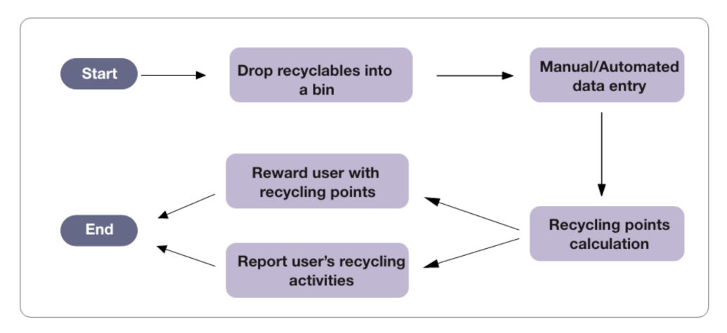
A waste management system is a tool that provides the ability for waste management organizations and government agencies to track recycling activities and assist communities in recycling. In this paper, we have studied a waste management system, where waste management organizations subscribe to bins and the system accounts for each bin. With the help of this system, the organizations (bin owners) are able to generate reports of each bin recycling activity. The reports contain information about the recycler, bin, recyclable items, and many more. The recycling activities in this system are tracked as follows:

Figure 1 shows the steps, where the recycler first drops their recyclable bags into the bin. Each bag has a unique barcode that identifies the recycler. The next step is to update the recyclable data in the system. This step can be done manually by the bin owner or automatically when the user drops the items. The following step is to calculate the user’s recycling points and reward them. The waste management organization has identified fraud activities in data entry steps, where illegal transactions are taking place. The recycler attempts to perform these illegal activities to either gain free recycling points or avoid government penalties for those who are required to recycle their own waste.

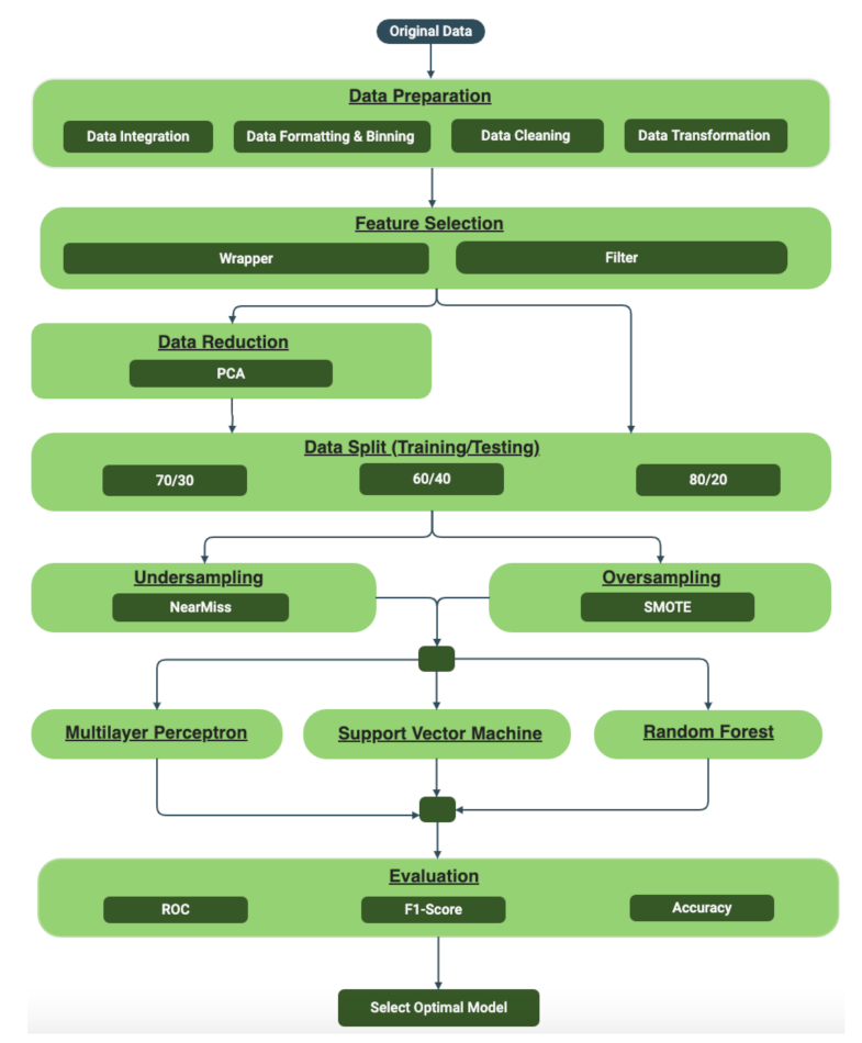
In this paper, we come up with a methodology for developing a machine learning model that can detect these activities. Figure 2 illustrates the steps involved in providing the optimal model.

2.1.1. Data Description

The data set used in this study is a private data set obtained from iCYCLE Malaysia, which is a Malaysian Waste Management Organization. It covers wider geographical areas. It contains waste collection data from different branches and countries. It has information about the recycler details, bin details, region, country, waste collection date and time, and recyclable details. These details provide the ability to analyze user recycling behaviors. The transactions are labeled as ’pending’ for suspicious, ’rejected’ for fraudulent, or ’approved’ for legitimate. The three labeled data sets were combined into one file after they were obtained from different sources. When evaluating the combined data set, the shape of the ’approved’ transactions is much more skewed than the other classes, ’pending’ and ’rejected’, due to the unequal class distribution. The file with ’approved’ transactions has 65702 observations while the ’rejected’ and ’pending’ have 14343 and 2732 respectively. The data attributes are listed in

Table 1. Dataset Attributes.

Attribute	Description
collection_date	Recyclables collection date
updated_date	Date on which the recyclables data is keyed in
transaction_id	Each transaction has unique ID
user_id	A unique ID of the user, who performs the transaction
user_email	Email of the user, who performs the transaction
user_client	Recycling organization, from which the user performs the transaction
user_joining_date	Date on which the user enrolled into the system
bin_name	Bin name that the user drops the recyclables into
bin_location_lat	Bin location (Latitude)
bin_location_lng	Bin location (Longitude)
item_name	Rrecyclable name
item_id	A unique identifier of the recyclable material
item_multiplier	A number that is multiplied by the recyclable weight or the number of recyclables to produce the recycling points (reward points)
recycling_points	Rewarding points
item_weight	Recyclables weight
number_of_items	The number of the recyclables in the transaction
updated_by	ID of the user, who keys in the recyclables data into the system
status	Transaction class (normal, abnormal, or fraud)
user_country	Country from which user has registered

.

The transactions contain details of the recycler, the bin, including its location, items dropped by the recycler, the person who sorts and processes the items, the collection dates of the items, the updating date on which the data is inserted into the system, and finally, the status of the transaction.

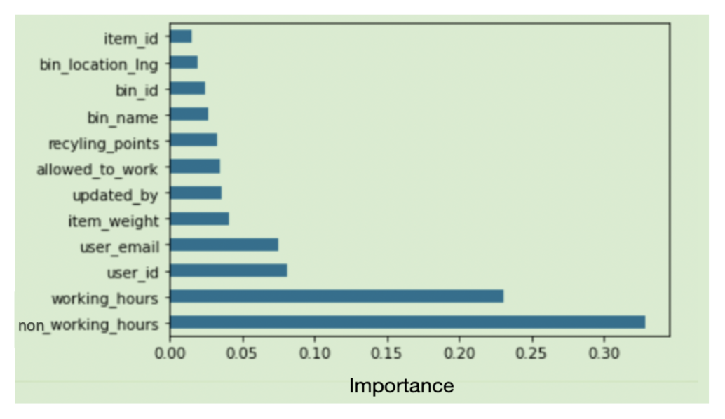
We performed exploratory analysis on the data, and we found that transaction time (working hours/non-working hours), user id, and item weight are the most important features of the output variable “status”. Figure 3 shows the most important attributes of the target variable.

When we examine the relationship between the target variable (status) and transaction time (hours), shown in the box plot distribution in Figure 4, we see that most of the ‘rejected’ transactions occur in the very early hours of the day. The distribution of the ‘approved’ transactions start from 9 in the morning to 7 in the evening. This interval time is considered the normal time for transactions to occur within the system. We can also see ‘approved’ transactions occurring at 0 h, which represents 12 midnight. According to the system expert, these transactions are normal as the system processes some transactions from the system logs daily at 12 midnight. ‘Pending’ transactions that could be either ‘approved’ or ‘rejected’ are distributed over the entire day. These transactions require more investigation by the system admin to determine their validity.

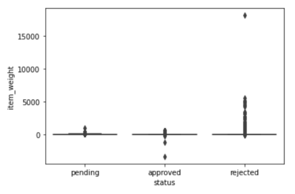
The item weight has an impact on determining whether the transaction is either ‘pending’, ‘approved’, or ‘rejected’. We can see in Figure 5 that most of the ‘rejected’ transactions have items with a very high weight, which is unusual for a recycler to recycle, for example, 1000 kg of iron.

2.1.2. Data Preparation

Before feeding the data into machine learning algorithms, basic data pre-processing is applied. The data is integrated, cleaned, and transformed. Features are explored and extracted. The steps, which were involved in the data preparation are described below.

• Data Integration: Before the data is subjected to further changes, the three data sources namely, ‘approved’, ‘pending’, and ‘rejected’ files, were combined into one file.
• Data Cleaning: Identifying the incorrect, incomplete, inaccurate, irrelevant, or missing parts of the data and then modifying, replacing, or deleting them according to the necessity is a very important task in data cleaning. There are many ways to tackle this issue. We performed data imputation for some of the missing values and also removed the rows with more than five missing values, where 24 rows were affected. For example, those rows that have missing values for the attributes bin ID, bin location, item ID, and item multiplier were removed. Other missing values of numerical attributes such as item weight and number of items were replaced with 0, which is based on expert domain consultation. The transaction items measured with weight has a 0 value for the number of items attribute and the one measured with quantity has a 0 value for the item weight attribute. In other words, each transaction can have only one item weight or a number of items attributes. For instance, a transaction with the item paper has a value of the item weight attribute and 0 for the number of items attribute. That is because the item paper is measured by its weight. On the other hand, the transaction with the item TV has a value of 0 for the item weight attribute as the item TV is measured by quantity.
  Additionally, some missing values were replaced with the most frequent values or the value of the row before. For example, the transactions with missing collection data are replaced with the collection date as the data set is sorted in descending order based on the collection date.
  For the missing values of the ’updated_by’ attributes, we performed three steps. Firstly, we separated the data set into multiple data sets based on user_country attribute. Then we grouped the transactions based on the updated_by value. Finally, we replaced the “NaN” value with the most frequent value of each data set.
• Data Formatting and Binning: Format consistency is another issue where the same value appears in different forms. For instance, the country of a recycler appears as either ’MY’ or ’+60’ for Malaysia. Based on our data exploratory and consulting with the domain expert, we found that most of the ’rejected’ transactions occurred outside of working hours. The transactions were categorized into three different groups. The three groups were identified as working_hours (during working hours), not_working_hours (out of working hours), and allowed_to_work (overtime). The hours of each group were advised by a domain expert.
• Data Transformation: As most machine learning algorithms cannot process categorical data, all categorical data is consolidated into an understandable numerical format.

2.1.3. Data Reduction and Feature Selection

We applied wrapper and filter methods to select those features, which contribute most to the prediction variable or output. We applied recursive feature elimination and feature importance using the ExtraTreesClassifier algorithm from the sikitlearn library. Both techniques produced almost the same result. We selected the first 12 important variables and then we applied correlation to detect variables with the same impact on the target. Based on the correlation result, only one feature is kept from a group of features that have the same impact on the target.

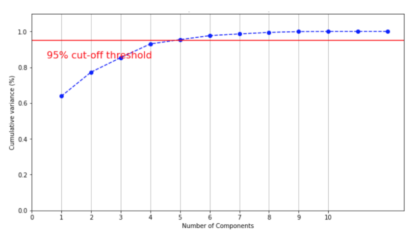
Dimension reduction is used to achieve data reduction. Principal component analysis (PCA) is used to find the suitable number of principal components. We set 5 as the number of the component parameters to be kept. In other words, we transform 20 variables of the original data set into a smaller one with 5 variables that still contains most of the information in the large set. Figure 6 shows that the 5 variables preserve 95% variance in the data.

2.1.4. Data Re-Sampling

The data set is highly imbalanced, where the distribution of examples across the known classes are biased or skewed. The legitimate ’approved’ transactions have a much bigger number than the other classes pending and ’rejected’. To treat the problem of class imbalance, re-sampling techniques were conducted in this research to overcome this issue. Oversampling is used to increase the minority occurrences and reduce the majority. The techniques will be applied to the training data set and prior to fitting the training data into a model. We conducted Synthetic Minority Oversampling Techniques (SMOTE) for oversampling and NearMiss for under-sampling. Figure 7 shows how the data is distributed before the data set is split into training and testing sets.

Table 2. Classes distribution of the original data set.

Origin Data (Training Data)
Classes Split(%) \ Class	Pending	Rejected	Approved
20/80	2186	11,474	52,609
30/70	1912	10,004	46,033
40/60	1639	8605	39,457

shows three splits we used in our experiments. The sampling techniques are applied only on the training data set.

Table 3. Classes distribution after applying over-sampling on the minority class.

Over-Sampling Technique on Training Data
Classes Split(%) \ Class	Pending	Rejected	Approved
20/80	11,400	11,474	52,609
30/70	10,000	10,004	46,033
40/60	8600	8605	39,457

shows the result after applying only oversampling on the minority class ‘pending’ using SMOTE.

Table 4. Classes distribution after applying under-sampling on the majority class and over-sampling on the minority class.

Under-Sampling and Over-Sampling Technique on Training Data
Classes Split(%) \ Class	Pending	Rejected	Approved
20/80	11,400	11,474	11,500
30/70	10,000	10,004	10,005
40/60	8600	8605	8700

shows the result after applying both under-sampling on the majority class ‘approved’ using NearMiss and oversampling on the minority class ‘pending’ using SMOTE.

2.1.5. Modeling

Classification models have a very important place in automated decision-making systems. The model helps to determine the features belonging to each class. There are many algorithms that simplify the classification process. They can give different results for different data sets. Based on our analysis with the help of the literature, three machine learning algorithms were prioritized. They are Random Forest, Support Vector Machine, and Multi-layer Perceptron Neural Network. We applied different parameters for each algorithm. The algorithms were applied to the re-sampling data. The optimal model is selected based on an appropriate performance metrices. We fed all the algorithms with data set shapes. Three different training and testing split ratios were applied with under-sampling, oversampling, or both. Additionally, we applied PCA in a few cases. We used Random Forest (RF) from the Scikit Learn Library; after tuning of n estimators, which is the number of decision trees in the forest, this value was set to 44. The Support Vector Machine (SVM) with RBF and Ploy Kernel Model from the Scikit Learn library was used to train the model with the penalty parameters. Since we are dealing with multi-class problems, we set the parameter decision_function_shape to two strategies: One-vs-Rest (OVR) and One-vs-One (OVO). For Multi-layer Perceptron, we used the MLPClassifier library from Scikit Learn. We trained the model with the default parameters and grid search. Activation functions such as ‘tan h’ and ‘relu’ were used in the grid search with different solvers. After tuning of n hidden layers, this value is set to three, where the first layer has 5, the second has 10 and the last has 5 nodes.

We have used the following packages, tools, and environments for the fraud detection model implementation: Anaconda, Imbalanced Learn, Jupyter Notebook, Matplotlib, Numpy, Pandas, Python 3.7, Scikit Learn, and Seaborn.

3. Results

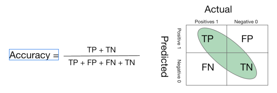
The performance of each model is measured, and its accuracy is evaluated. The performance measures adapted in this model are: accuracy, F1-Score, and AUC-ROC Curve. The accuracy calculates the number of correct predictions made by the model over all kinds of predictions made.

In the numerator, correct predictions (True positives and True Negatives are marked with green area in Figure 8) are placed and in the denominator, both correct and incorrect predictions made by the algorithm is placed. The F1-score, which is the harmonic mean of precision and recall, is also used as a measure to evaluate our model. Therefore, it considers both false positives and false negatives. Especially in cases of irregular class distribution, looking at the F1-score may be more useful than looking at the accuracy. The advantage of using this metric is in identifying the model with best precision and recall at the same time. For a multi-class classification problem, F-1 score per class in a one-vs-rest manner is calculated instead of overall F-1 score. We applied ’weighted’ to the parameter average to calculate the single average score. The calculation of the F-1 score for each class is as follows:

$$\begin{array}{c}\hfill F-1Score(class=x)=2\ast \left[Precision\right(class=x)\ast Recall(class=x\left)\right]/\\ \hfill Precision(class=x)+Recall(class=x)\end{array}$$

(1)

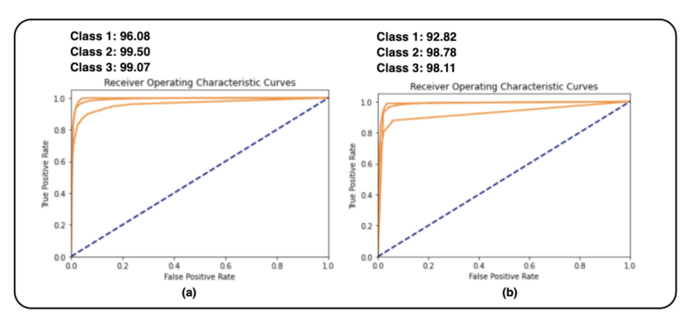
For the imbalanced class problem, AUC-ROC curve is used to measure how well the models can predict minority class ’pending’ correctly. An excellent model has an AUC near to 1, which means it has a good measure of separability. Figure 9, Figure 10 and Figure 11 of the AUC-ROC curves show the performance of different models with different algorithms and parameters.

4. Discussion

Table 5. The performance of Multi-layer Perceptron classifiers.

Parameters	PCA	Variables	Sampling	(%)	Score	Macro-Averaging
Hidden layers: 3 Number of neurons: 100 (25,50,25) Activation function: Relu Data split: 40/60	Yes	5	Over Under	83.48	79.11	82.73
Hidden layers: 3 Number of neurons: 100 (25,50,25) Activation function: Tanh Data split: 40/60	No	12	Over	93.50	93.55	98.93
Hidden layers: 1 Number of neurons: 200 Activation function: Relu Data split: 40/60	No	12	Over Under	91.62	90.14	92.52
Hidden layers: 1 Number of neurons: 100 Activation function: Identity Data split: 40/60	Yes	5	Over	91.72	93.23	91.66
Hidden layers: 2 Number of neurons: 100 (50,50) Activation function: Identity Data split: 40/60	Yes	5	Over	91.38	88.27	92.13
Hidden layers: 3 Number of neurons: 20 (5,10,5) Activation function: Identity Data split: 20/80	No	12	Over	86.73	86.38	88.32
Hidden layers: 3 Number of neurons: 20 (5,10,5) Activation function: Identity Data split: 40/60	No	12	Over Under	89.43	78.62	88.54

,

Table 6. The performance of Random Forest classifiers.

Parameters	PCA	Variables	Sampling	(%)	Score	ROC (Macro-Averaging)
Number of trees: 44 Data split: 40/60	No	12	Over Under	84.67	83.66	81.37
Number of trees: 50 Data split: 30/70	No	12	Over Under	79.83	77.34	82.68
Number of trees: 44 Data split: 40/60	Yes	5	Over	85.38	81.74	86.27
Number of trees: 34 Data split: 20/80	No	12	Over	84.71	81.92	84.29
Number of trees: 44 Data split: 40/60	No	12	Over	96.33	95.20	98.92
Number of trees: 44 Data split: 30/70	Yes	5	Over Under	77.64	73.48	69.92

and

Table 7. The performance of Support Vector Machine classifiers.

Parameters	PCA	Variables	Sampling	(%)	F1-Score	ROC (Macro-Averaging)
Kernel: Poly Degree: 3 Decision function: OVA Data split: 40/60	No	12	Over Under	79.29	71.56	77.64
Kernel: Poly Degree: 3 Decision function: OVO Data split: 30/70	Yes	5	Over	72.93	70.81	79.37
Kernel: Poly Degree: 3 Decision function: OVO Data split: 40/60	Yes	5	Over	66.41	68.62	62.88
Kernel: RBF Degree: 3 Decision function: OVO Data split: 40/60	No	12	Over	96.20	96.20	88.55
Kernel: RBF Degree: 3 Decision function: OVO Data split: 30/70	Yes	5	Over	70.38	69.47	74.66
Kernel: RBF Degree: 3 Decision function: OVA Data split: 40/60	No	12	Over Under	88.76	81.51	87.51

list the performance of multi-layer perceptron, support-vector machines, and random forest as classifiers for waste management fraud detection systems. In general, all these models can be used as classifiers for waste management fraud detection.

However, the experimental results showed that the models have difficulties in correctly predicting ‘pending’ transactions compared to ‘approved’ and ‘rejected’ ones. For example, the SVM model with RBF kernel poorly detects ‘pending’ transactions with ROC macro-averaging of 78.43% compared to ‘rejected’ and ‘approved’ transactions with ROC macro-averaging of 85.76% and 86.90% respectively.

As shown in Figure 2, the experiments were done with and without data reduction. Experimental results indicate that data reduction has less impact on the result of each model. Based on the results, as shown in Table 5, Table 6 and Table 7 random forest classifier with an accuracy of 96.33%, F1-Scor of 95.20%, and ROC (micro-average) of 98.92% is selected as the optimal model.

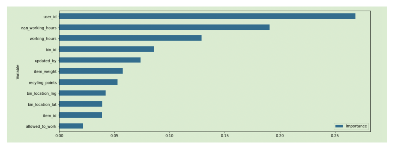
A model interpretation was done on the selected optimal model. As we can see in Figure 12, user_id, non_working_hours, and working_hours are the most contributing attributes to the outcome of the optimal model.

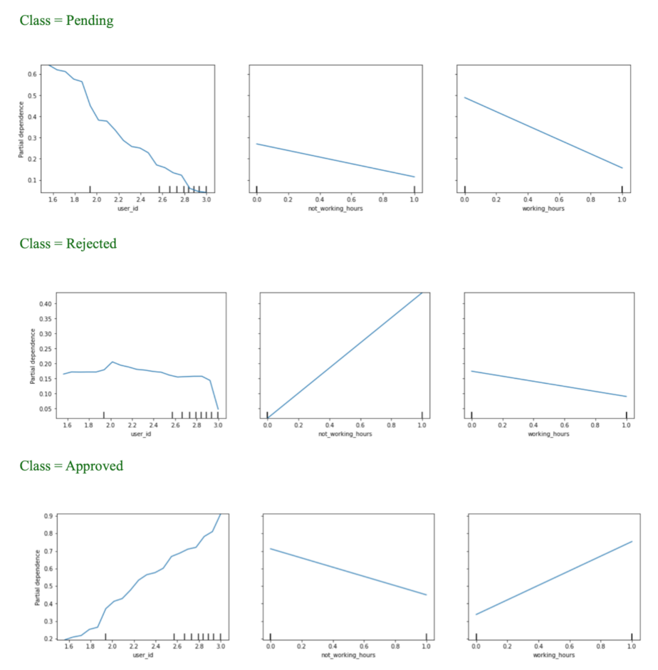
The following partial dependence plots of the optimal model show the relationship between the most contributing variables and target variable ‘status’.

From Figure 13, we can tell that the value of the dependent variable is higher than the lower value of the variable ‘user_id’ with the classes ‘pending’ and ‘approved’. Also, the higher value of the variable ‘non_working_hours’ leads to a ‘rejected’ class. Similarly, the higher value of the variable ‘working_hours’ leads to higher possibility of the approved class.

No comparison was conducted between our optimal model and other fraud detection models introduced by other researchers as waste management system data set is different from the datasets of other domains.

5. Conclusions

Fraud detection systems have been employed in several domains but has not been attempted for waste management system domain. This research has focused on applying different machine learning techniques such as multi-layer perceptron, random forest, and support vector machines as classifiers to detect fraudulent transactions, by utilizing the real dataset from a recycling organization. Experimental results show that by applying the appropriate pre-processing techniques, sampling techniques for addressing the imbalanced data-set problem, and by tuning of parameters, all the proposed models can be used for classifying ‘approved’, ‘rejected’, and ‘pending’ transactions during recycling process activities. These different machine learning models have been analysed based on different metrics such as accuracy, F1-score, and AUC-ROC curve.

The proposed models can be a solution that can provide the recycling organisations with an ability to detect fraudulent activities during their waste collection process activities. Even though the models are trained on the specific recycling organization dataset, this includes the data from multiple branches of the organization in different countries, which cover wider geographical areas. In general, these models can also be applied in other waste management systems. However, these models can be further evaluated using multiple datasets from different organisations to validate their generalization abilities.

References

- Internet Fraud. Available online: https://en.wikipedia.org/wiki/Internet_fraud (accessed on 3 May 2021).
- Hao, W.; Jiang, C. Local Nuances of Authoritarian Environmentalism: A Legislative Study on Household Solid Waste Sorting in China. Sustainability 2020, 12, 2522. [Google Scholar] [CrossRef] [Green Version]
- Majhi, S.K.; Bhatachharya, S.; Pradhan, R.; Biswal, S. Fuzzy clustering using salp swarm algorithm for automobile insurance fraud detection. J. Intell. Fuzzy Syst. 2019, 36, 2333–2344. [Google Scholar] [CrossRef]
- Gao, J.; Zhou, Z.; Ai, J.; Xia, B.; Coggeshall, S. Predicting Credit Card Transaction Fraud Using Machine Learning Algorithms. J. Intell. Learn. Syst. Appl. 2019, 11, 33–63. [Google Scholar] [CrossRef] [Green Version]
- Aljawarneh, S.; Aldwairi, M.; Bani, M. Anomaly-based intrusion detection system through feature selection analysis and building hybrid efficient model. J. Comput. Sci. 2018, 25, 152–160. [Google Scholar] [CrossRef]
- Makki, S.; Assaghir, Z.; Taher, Y.; Haque, R.; Hacid, M.; Zeineddine, H. An Experimental Study With Imbalanced Classification Approaches for Credit Card Fraud Detection. IEEE Access 2019, 7, 93010–93022. [Google Scholar] [CrossRef]
- Thennakoon, A.; Bhagyani, C.; Premadasa, S.; Mihiranga, S.; Kuruwitaarachchi, N. Real-time Credit Card Fraud Detection using Machine Learning. In Proceedings of the 9th International Conference on Cloud Computing, Data Science & Engineering (Confluence), Noida, India, 10–11 January 2019; pp. 488–493. [Google Scholar] [CrossRef]
- Zhou, H.; Sun, G.; Fu, S.; Jiang, W.; Xue, J. A Scalable Approach for Fraud Detection in Online E-Commerce Transactions with Big Data Analytics. Comput. Mater. Contin. 2019, 60, 179–192. [Google Scholar] [CrossRef] [Green Version]
- Kim, Y.J.; Baik, B.; Cho, S. Detecting financial misstatements with fraud intention using multi-class cost-sensitive learning. Expert Syst. Appl. 2016, 62, 32–43. [Google Scholar] [CrossRef]
- Sevdalina, G.; Maya, M.; Velisar, P. Using neural network for credit card fraud detection. AIP Conf. Proc. 2019, 2159, 030013. [Google Scholar]
- Mohamed, L.; Hamad, T.; Sean, Z.E. Towards blockchain-based urban planning: Application for waste collection management. In Proceedings of the 9th International Conference on Information Systems and Technologies, Cairo, Egypt, 24–26 March 2019; pp. 1–6. [Google Scholar] [CrossRef]
- Aazam, M.; St-Hilaire, M.; Lung, C.; Lambadaris, I. Cloud- based smart waste management for smart cities. In Proceedings of the 2016 IEEE 21st International Workshop on Computer Aided Modelling and Design of Communication Links and Networks (CAMAD), Toronto, ON, Canada, 23–25 October 2016; pp. 188–193. [Google Scholar] [CrossRef]
Figure 1.
Waste management system flow.
Figure 2.
Steps involved in optimal model selection.
Figure 3.
Most important attributes to the target variable status.
Figure 4.
Relationship between target variable and transaction time.
Figure 5.
Relationship between target variable and item weight.
Figure 6.
The number of components needed to explain 95% variance.
Figure 7.
Classes distribution of the original data set.
Figure 9.
AUC-ROC curve performance of three MLP models with different parameters. (a) MLP with Tanh as an activation function with 3 hidden layers (25, 50, 25). (b) MLP with Relu as an activation function with 3 hidden layers (50, 100, 50). (c) MLP with Identity as an activation function with 3 hidden layers (25, 50, 25).
Figure 10.
AUC-ROC curve performance of two random forest models with different parameters. (a) Random forest with 44 trees and using the oversampling technique for the minority class. (b) Random forest with 20 trees and using the oversampling technique for the minority class and under-sampling technique for the majority class.
Figure 11.
AUC-ROC curve performance of two support vector machine models with different parameters. (a) Support Vector Machine with poly kernel, one-vs-one function shape, and oversampling technique. (b) Support Vector Machine with RBF kernel, one-vs-one function shape, and oversampling technique.
Figure 12.
Variable importance for the optimal model.
Figure 13.