Global Stock Selection with Hidden Markov Model

1
Department of Mathematics and Statistics, Youngstown State University, 31 Lincoln Ave., Youngstown, OH 44503, USA
2
Ned Davis Research Group, 600 Bird Bay Drive West, Venice, FL 34285, USA
*
Author to whom correspondence should be addressed.
Risks 2021, 9(1), 9; https://0-doi-org.brum.beds.ac.uk/10.3390/risks9010009
Submission received: 6 November 2020
/
Revised: 2 December 2020
/
Accepted: 11 December 2020
/
Published: 31 December 2020
(This article belongs to the Special Issue Portfolio Optimization, Risk and Factor Analysis)
Abstract
:Hidden Markov model (HMM) is a powerful machine-learning method for data regime detection, especially time series data. In this paper, we establish a multi-step procedure for using HMM to select stocks from the global stock market. First, the five important factors of a stock are identified and scored based on its historical performances. Second, HMM is used to predict the regimes of six global economic indicators and find the time periods in the past during which these indicators have a combination of regimes that is similar to those predicted. Then, we analyze the five stock factors of the All country world index (ACWI) in the identified time periods to assign a weighted score for each stock factor and to calculate the composite score of the five factors. Finally, we make a monthly selection of 10% of the global stocks that have the highest composite scores. This strategy is shown to outperform those relying on either ACWI, any single stock factor, or the simple average of the five stock factors.
1. Introduction
Predicting the stock price is enormously challenging Andriosopoulos et al. (2019); de Prado (2018). Generally, stock price is very sensitive with respect to numerous (or even infinite number of) social and economic factors, many of them are not only hidden to observers but also highly uncertain in nature, for example, economics condition, company’s policies and decision making mechanisms, social trends Ball (2013); Preis et al. (2013) and political indications Alloway (2019). Moreover, the stock price also reflects in some ways the collective behavior of a large number of traders, who, in turn, are driven by their psychology and other personal details.
Computational modeling, specifically machine-learning (ML) methods, is a primary quantitative approach for stock price prediction Andriosopoulos et al. (2019); de Prado (2018); Markowitz (1952). Such a data-driven approach is enormously useful for a very wide range of disciplines, ranging from financial modeling de Prado (2018) to cheminformatics Brown (1998); Engel (2006) and materials science Huan et al. (2015); Kim et al. (2018). Within the area of stock market prediction, many typical modeling and ML algorithms, for example, artificial neuron network Liu and Yeh (2017); Thawornwong and Enke (2004), support vector machine Fan and Palaniswami (2001); Huang (2012), differential evolution Yu et al. (2016), genetic algorithm Huang (2012), and particle swarm optimization Nenortaite and Simutis (2004) have been used. A large number of features, including book value-to-price ratios and return on equity, etc. Liu and Yeh (2017), return on capital, profitability, and leverage, etc. Fan and Palaniswami (2001), share price rationality, and profitability etc. Huang (2012), price ratio and profitability, etc. Yu et al. (2016), were used as the input of the ML models. Recently, Google counting and search trending Ball (2013); Preis et al. (2013) and Trump’s Tweet Alloway (2019) were also suggested to be good features. For all the disciplines in which ML approaches are used, features (or sometimes referred to as fingerprints and attributes) constructions and selections are critically important Huan et al. (2015); Kim et al. (2018); Liu and Wang (2019).
Hidden Markov model (HMM) is an ML method for recognizing patterns in stochastic processes, for example, time series. HMM was traditionally known for numerous applications in reinforcement learning and pattern recognition such as speech recognition Rabiner and Juang (1992), handwriting recognition Bunke et al. (1995), musical score following Pardo and Birmingham (2005), partial discharges Satish and Gururaj (1993), and bioinformatics Li and Stephens (2003); Yoon (2009). In economics and finance, HMM has recently been emerging Mamon and Elliott (2007) with applications in modeling foreign exchange data Idvall and Jonsson (2008), forecasting stock price of interrelated markets Hassan and Nath (2005), predicting the regimes of market turbulence, inflation and industrial production index Kritzman et al. (2012), predicting the regimes of some economic indicators and selecting stocks Nguyen and Nguyen (2015); Nguyen (2017b), modeling interest rates Nguyen et al. (2018) and mortgage backed securities Nguyen (2017a), analyzing stock market trends Kavitha et al. (2013), predicting the S&P 500 daily prices and developing a strategy to trade stock Lajos (2011). HMM is particularly useful for regime-switching models Hamilton (1989), an important class of financial models within which market regimes (cycles) are modeled. In such a model, the observation variables are generated by an autoregression model, of which the parameters were optimized by a discrete Markov chain.
Since HM is a pattern recognition model, it is feasible to be used to detect economic regimes, which have strong effect on stocks’ performances. In our previous paper Nguyen and Nguyen (2015), we used HMM to predict regimes of four macroeconomic indicators, then analyzed five stock return factors to select the top 10% stocks in the S&P 500 index for our monthly trading portfolio. However, the stock market depends on many other global economic indicators. Nijam and Musthafa (2015) investigated the relationships between the All share price index of the Colombo stock exchange and five macroeconomic variables. They found that the macroeconomic variables and the stock market index in Sri Lanka are significantly related. Khan and Khan (2018) concluded that stock prices of Karachi Stock Exchange in the long term are significantly affected by the three economic indicators: money supply, exchange rate, and interest rate. The interactions among economic indicators and stock returns in Greece were explored in Hondroyiannis and Papapetrou (2001). Based on the empirical study, stock returns do not lead to changes in real economic activities while the macroeconomic activities and foreign stock market returns only partially affect stock market movements. The paper indicated that oil price changes explicated stock price movements and have a negative impact on macroeconomic activities. The effects of macroeconomic variables on stock prices’ performances in the U.S. and Japan were investigated in Macmillan (2009). The papers showed that the macroeconomic indicators explained stock prices in different countries. Therefore, we want to expand the application of HMM in stock trading Nguyen and Nguyen (2015) to a broader market using more macroeconomics’ indicators.
In the paper, we use HMM to predict the economic regimes, based on which global stocks are evaluated and selected for optimizing the portfolio. While applications of HMM in local and national stock trading have been demonstrated Nguyen and Nguyen (2015), hidden factors driving global stocks are different and generally far more complicated. In Nguyen and Nguyen (2015) we investigated the effects of the four economics’ indicators: inflation, industrial production index, stock market index, and market volatility to performances of S& P 500 stocks. In the paper, we will expand to the global stock market, the All country world index. Therefore, we will choose the six macroeconomic indicators that have the most influence on the global stocks: inflation, production, sentiment, market, debt, and inflation expectation. The indicators we suggested in Sanborn et al. (2017).
The paper starts with Section 2 for a brief introduction of HMM. In Section 3, we introduce the All country world index (ACWI) and six global economic indicators, while five factors that effectively represent performances of the stocks are discussed in Section 4. Results of using HMM for global stock selection and portfolio optimization are discussed in Section 5. Results are presented in Section 6. The paper is closed with conclusions given in Section 7.
2. Hidden Markov Model
The mathematical foundations of HMM were developed by Baum and Petrie in 1966 Baum and Petrie (1966), followed by a maximization method, developed in 1970 for calibrating model parameters using a single observation sequence Baum et al. (1970). Methods for training HMM with and without the assumption of independent (multiple) observations were introduced in 1993 Levinson et al. (1983) and 2000 Li et al. (2000), respectively. We present some basic notations of the HMM in Table 1.
As summarized in Table 1, the parameters of an HMM are the constant matrix A, the observation probability matrix B, and the vector p, given in a compact notation as If the observation probability assumes the Gaussian distribution then , where and are the mean and standard deviation of the distribution corresponding to the state , respectively. Then, the parameters of HMM are
where and are vectors of means and variances of the Gaussian distributions, respectively. In this paper, we assume that the probability of observation in a given state follows a normal distribution with mean and standard deviation .
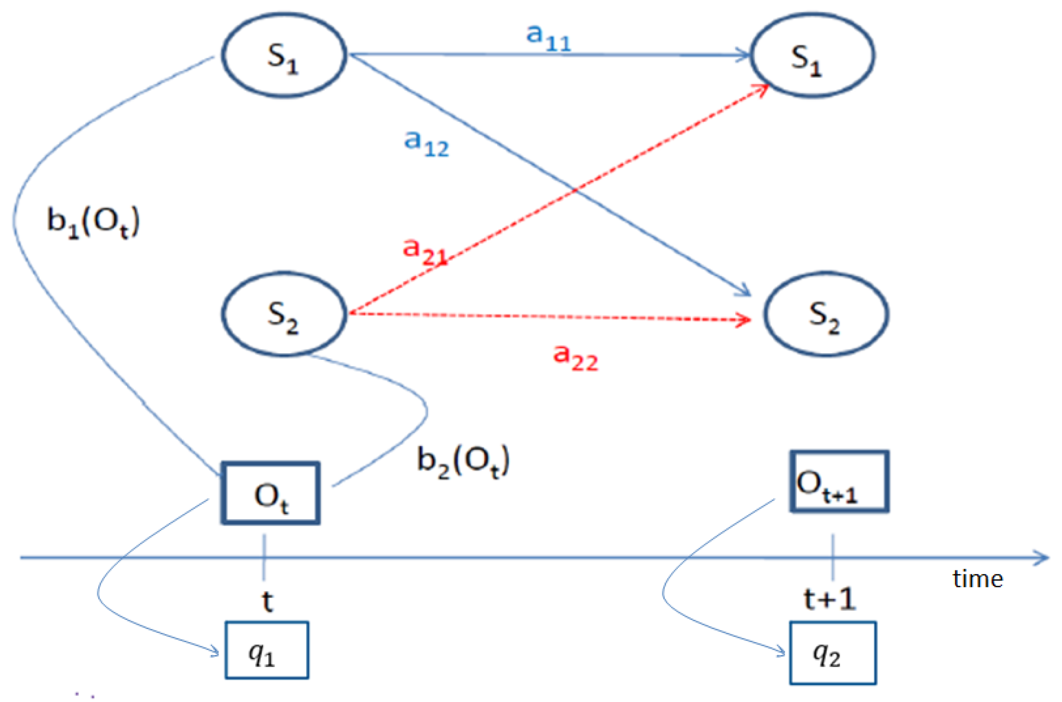
Figure 1 displays the HMM with two states. It shows elements of the transition matrix A, observation probability matrix B, and the vector initial probability p.
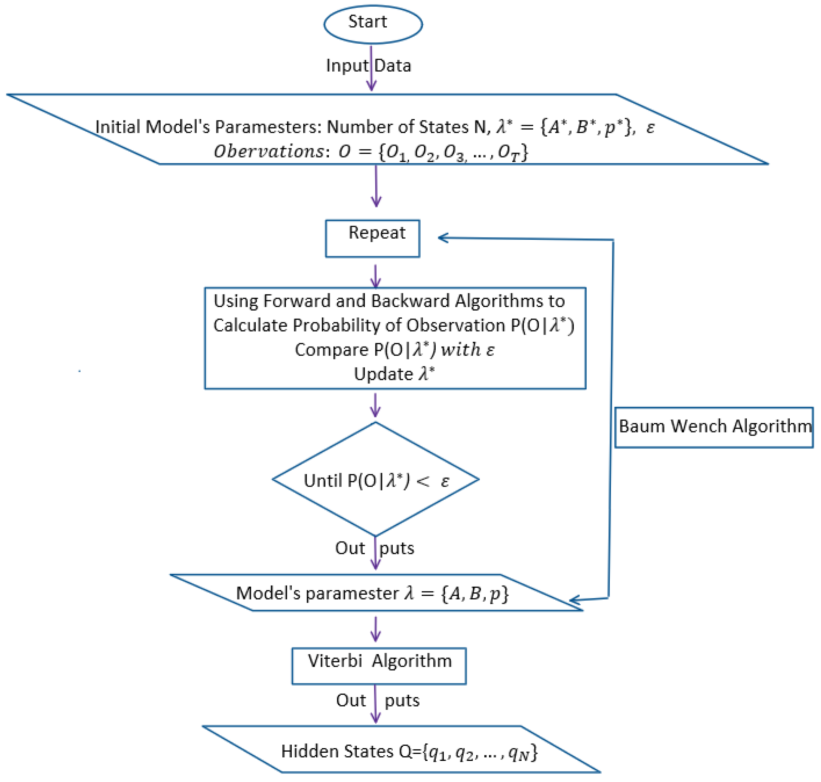
The process of using HMM for a single observation sequence can be explained in Figure 2. More details about the HMM can be found in References Baum and Petrie (1966); Nguyen (2017a).
3. All Country World Index and Global Economic Indicators
3.1. All Country World Index
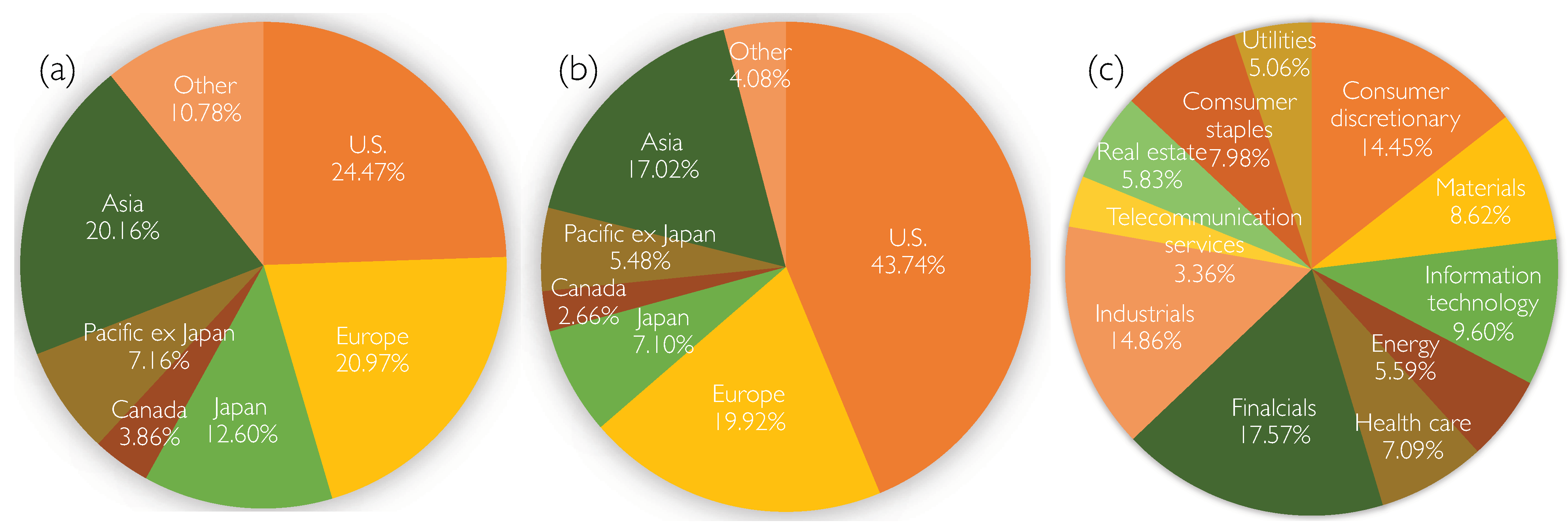
All country world index (ACWI) was developed and maintained by Morgan Stanley Capital International (MSCI). ACWI consists of large- and mid-cap representation across 23 developed-market and 24 emerging-market countries. In 2017, the index had about 2490 constituents (or stocks), which cover approximately 85% of the global investable equity opportunity set. The distribution of ACWI by physical location is given in Figure 3a, showing that the U.S. stock market contributes almost one-quarter of ACWI while each of the following entities, i.e., Europe and Asia, represents one-fifth of the stock universe.
There are many stocks that are trading in the U.S. market but issued by companies located outside the U.S., making the U.S. the biggest stock market in the world. Figure 3b provides the distribution of the ACWI by stock market cap in August 2017, showing that the U.S. stock market consumes almost a half of the ACWI, and the runner-ups are Japan, U.K., China, and France, each of which allocates less than ten percent of the market cap. Stocks that have big market caps are Apple, Microsoft, Amazon, MSCI India ETF, and Facebook. Figure 3c displays the distribution of the ACWI by sectors. The financial sector is the leading constituent of ACWI, which is followed by the industrial sector. The number of ACWI stocks changes over time, i.e., some new stocks will be issued and added each year.
3.2. Global Economic Indicators
We chose six main global macroeconomic variables that have significant impacts on the global stock market for this study. They are inflation, production, sentiment, market, debt, and inflation expectation, as summarized in Table 2.
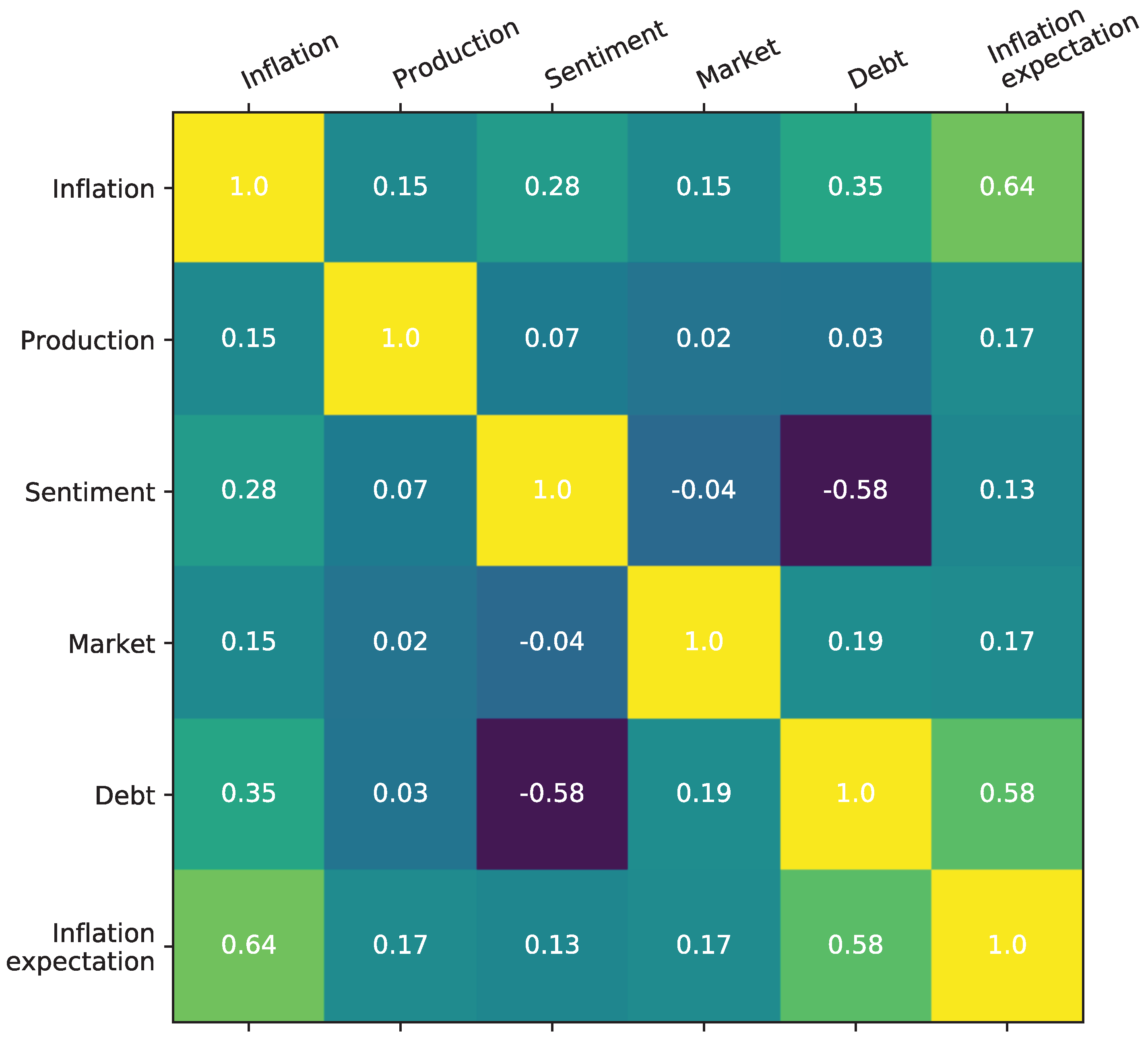
We used the Pearson correlation test in R to calculate the correlations of the six macroeconomics indicators. The correlation coefficients given in Figure 4 are mostly weak and moderate, indicating that the indicators are independent in representing the global economics. These indicators were used to identify the economic regimes, the most influential factor determining the nature and the dynamics of the stocks factor returns Sanborn et al. (2017).
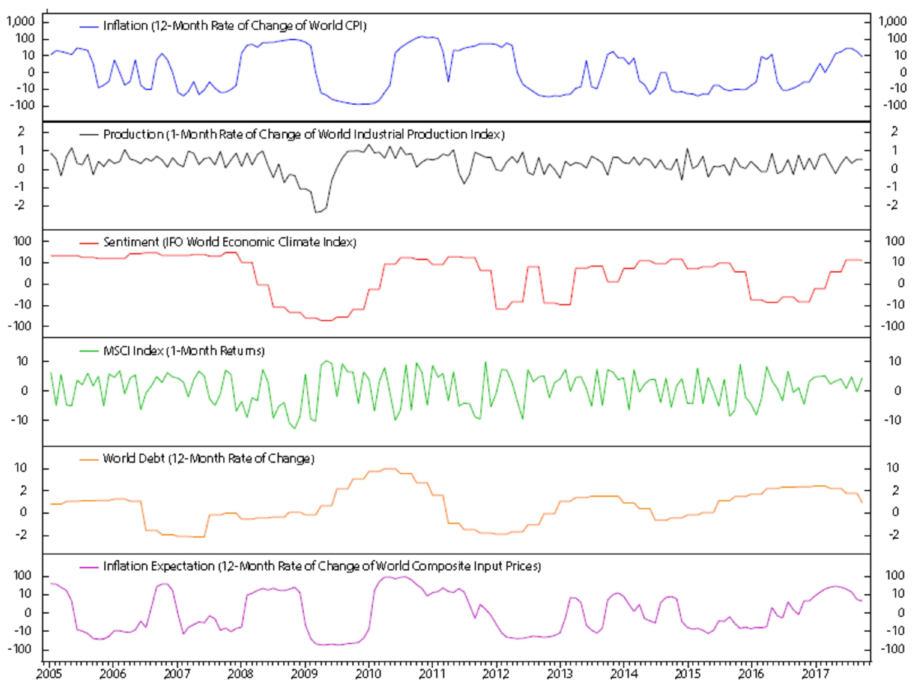
Monthly data of these indicators is available (see Figure 5), and we used their monthly changes or yearly changes as input data for our model.
4. Stock Factors
There are numerous stocks factors, which perform significantly differently in various macroeconomic regimes. This paper aims at selecting the best stock factors given the current economic environment, thus improving our portfolio performances. Investors have analyzed many criteria to choose the most important factors. Graham Graham (2003) suggested three factors that affect the stock market performances, including real growth, inflationary growth, and speculative growth. Researchers at Ned Davis Research Group Sanborn et al. (2017) examined about two hundred factors and narrowed them down to the five most important factors, including free cash flow/enterprise value, shareholder yield, lower accruals ratio, operating cash flow/assets, and price momentum. Based on the suggestions and our own analysis of the ACWI, we chose five stock factors for the world stock selection, which are (1) free cash flow/enterprise value, (2) earnings/price, (3) sales/enterprise, (4) long-term sales growth, and (5) long-term earning per share growth. The definitions of the factors are given in Table 3.
5. Global Stock Selection Using HMM
5.1. Stock Factors Scoring
A simple measure of the stock performance is the average score, defined as the equal weighted average of five factors scores of each of the stock in consideration. The average score is not ideal for stock selection because, in general, each factor has different effects on the stock price. We introduced a new multi-step procedure for global stock selection. Our procedure involves (1) using HMM to find regimes of the six global economic indicators, (2) analyzing the stock performance in the identified regimes, (3) assigning weight for the stock factors, (4) determining the (composition) weighted score of the stocks, and (5) selecting the top 10% for trading.
5.2. Regime Detection Using HMM
In the second step, HMM was used to detect the regimes of the six global economic indicators, the data of which is shown in Figure 5. Note that we consider monthly changes of production, market, and debt, and yearly changes of inflation and inflation expectation. For the sentiment data, we used the original data. The monthly changes or yearly changes was calculated by
where is observation data at time t, ( for monthly changes, and for yearly changes). We used these returns of the economic indicators to avoid dealing with different units of the data.
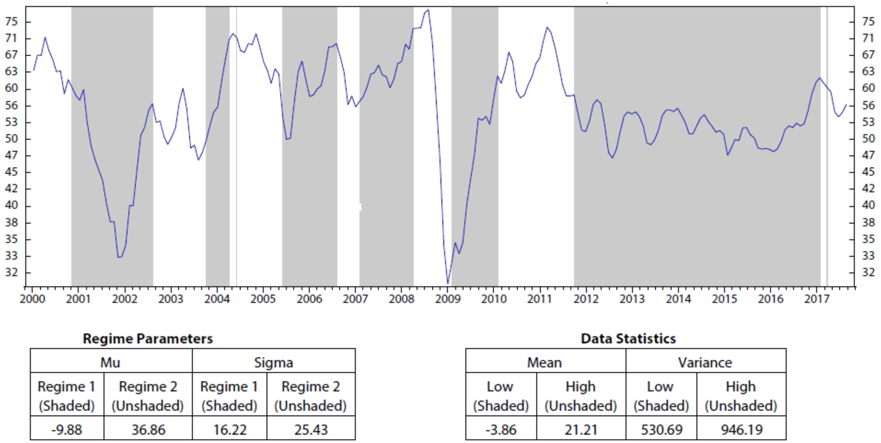
We assumed that the global economics has two regimes, regime 1 with low returns and regime 2 with high returns. Another assumption is that the observation probability of each indicator on a given regime follows a normal distribution with mean and standard deviation . At the end of each month, we used the Baum–Welch algorithm of the HMM to find its parameters, where , and A is a transitional probability matrix. Two ratios, i.e., and , were assigned to two economic regimes, the lower ratio for regime 1 and the higher for regime 2. In reality, in regime 1, the indicator has a lower and higher than that of regime 2. In a special case when one regime has a lower but also a lower than the other, regime 1 will have a lower ratio of the to its . After each month, we updated data and re-calibrated model parameters, predicting the economic indicators regimes, and keep moving on. Thus, we will not have the same regimes of economic indicators each month. In Figure A1, Figure A2, Figure A3, Figure A4, Figure A5 and Figure A6 in Appendix A, we present the regimes predicted for six global economic indicators, including inflation, production, sentiment, market (MSCI world index), debt, and inflation expectation, respectively, using monthly data from December 1999 to August 2017.
5.3. Stock Composition Scores
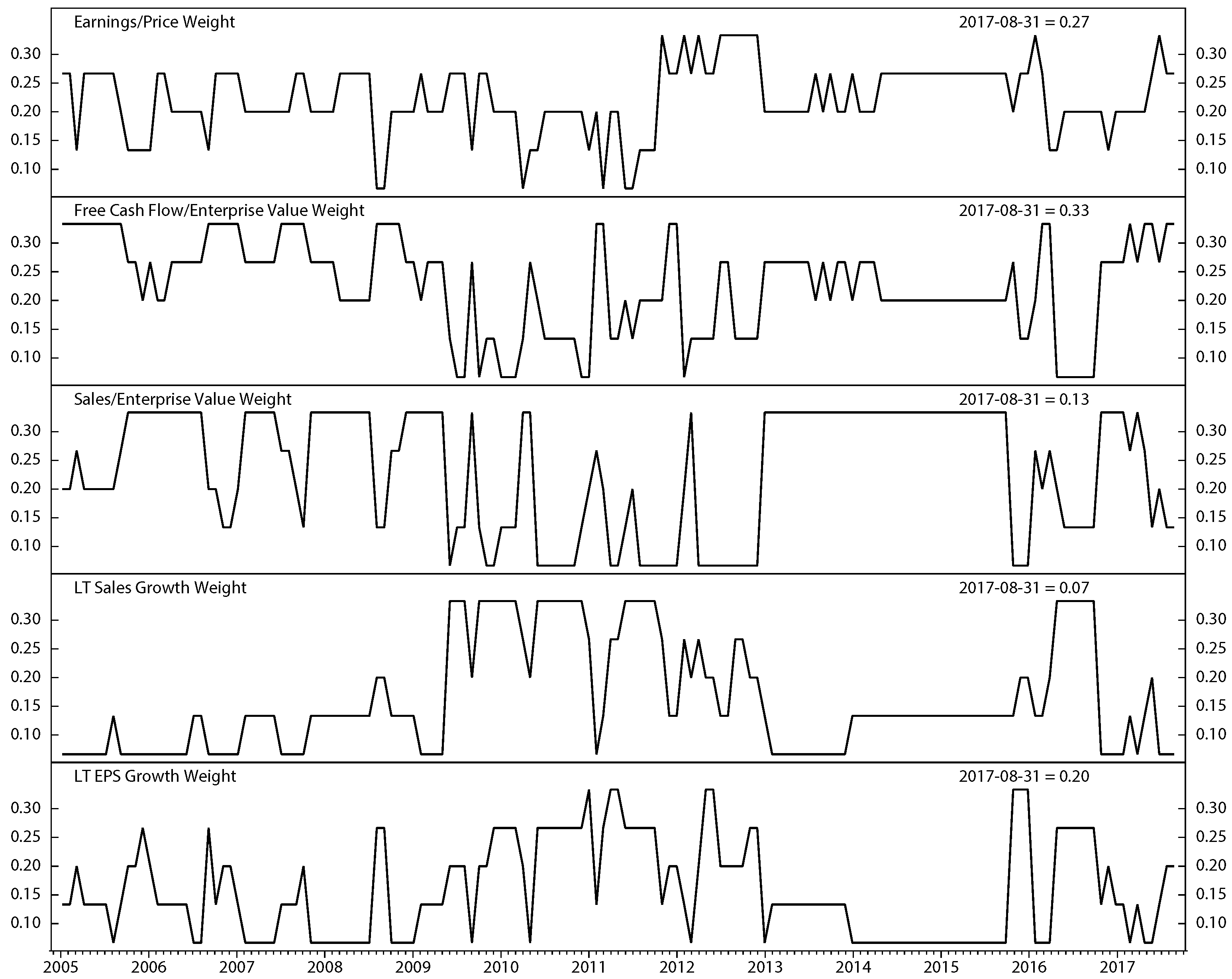
In Section 5.2, the regimes of the six global economic indicators, including inflation, production, sentiment, market, debt, and inflation expectation, were predicted by HMM using historical data up to the recent month. Then, we predict the regime of the indicators in the next month and then looked back at historical data to find similar regimes of these six variables. For example, if the predicted regimes of the next month (for inflation, production, sentiment, market, debt, and inflation expectation) are (1, 1, 2, 2, 1, 1), we looked for the months in the past when six indicators have the same regimes (1, 1, 2, 2, 1, 1). We then checked the performance of each stock factor (defined in Section 4) in the period of three months after each similar set of regimes. Based on the performances, we ranked the factors from 1 to 5. The weight of each factor was calculated by taking its rank divided by 15, the sum of all the possible ranks. The obtained weights of the five stock factors are shown in Figure 6.
The composite score of each stock was calculated by the summation of the products of its factor weight with the corresponding score. The composite scores range from 1 to 100. We selected 10% of the ACWI, which is about 250 stocks in 2017, with the highest composite score for our portfolio. To make a stock selection for the next month, we updated data and repeated the selection process. Note that each month we will calibrate new model parameters, predicting new economic regimes, and making a new stock selection. We will sell stocks that are no longer in our new list and buy the new stocks that are selected.
6. Results and Discussions
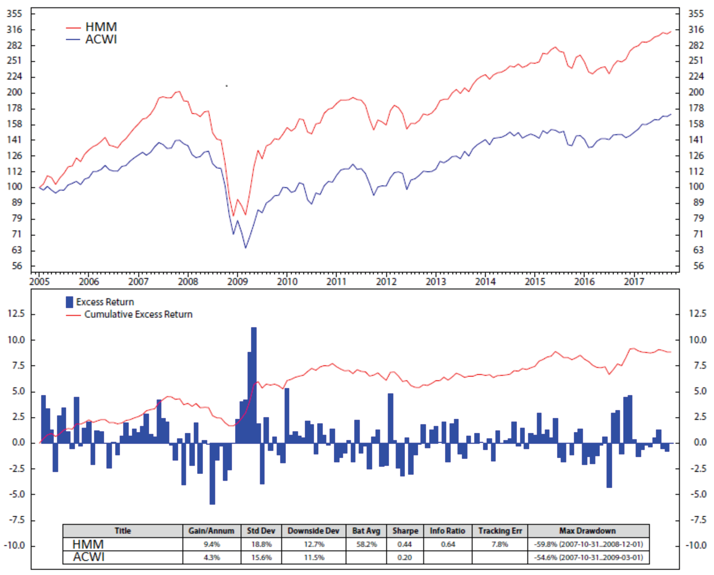
Figure 7 shows the monthly performances of our global stock portfolio compare to the whole ACWI from January 2005 to September 2017.
Among some model performances examined in Figure 7, batting average is a statistical measure used to evaluate our investment model ability to meet or beat the benchmark ACWI. The batting average was calculated by dividing the number of months within which the single factor portfolio beats or matches the ACWI by the total number of months in the period under consideration and multiplying the result with 100. In other words, the batting average is the percentage of the time within which the single factor portfolio returns meet or exceed the ACWI returns. Another performance is tracking error, measuring the consistency of excess returns. Tracking error was computed by taking the difference between the single factor portfolio return and the benchmark ACWI return every month, and then calculating how volatile that difference is. Tracking error is also useful in determining just how “active” a model strategy is. The lower the tracking error, the closer the model follows the benchmark, while the higher the tracking error, the more the model deviates from the benchmark. The Sharpe ratio is defined as the ratio between the mean of the excess of the asset return over the benchmark ACWI return and the standard deviation of the excess return. This is a measure of how well the return compensates the investor for the risk, thus the higher the Sharpe ratio, the better the stock in terms of return/risk balance. Figure 7 shows that with an initial investment of $100.00 in January 2005, we gain $316.00 in September 2017 using the HMM, about 76% higher than the gaining of $178.00 of ACWI. Information shown in the bottom table of Figure 7 also indicates that our HMM portfolio outperforms the benchmark ACWI.
We went further by comparing the performance of our portfolio using HMM with the two common stock selection methods, i.e., a single factor method and the equal weighted method. In the single factor method, stocks are selected based on scores of a single stock factor. In the equal weighted method, stocks are selected using the average score of the five stock factors, as explained in Section 5.1. Each month, we chose the top 10% stocks that have the highest scores. For the next month, we updated data and repeated the process to make a new portfolio. We sold ones that are not on the elected list while buying the newly-entered ones.
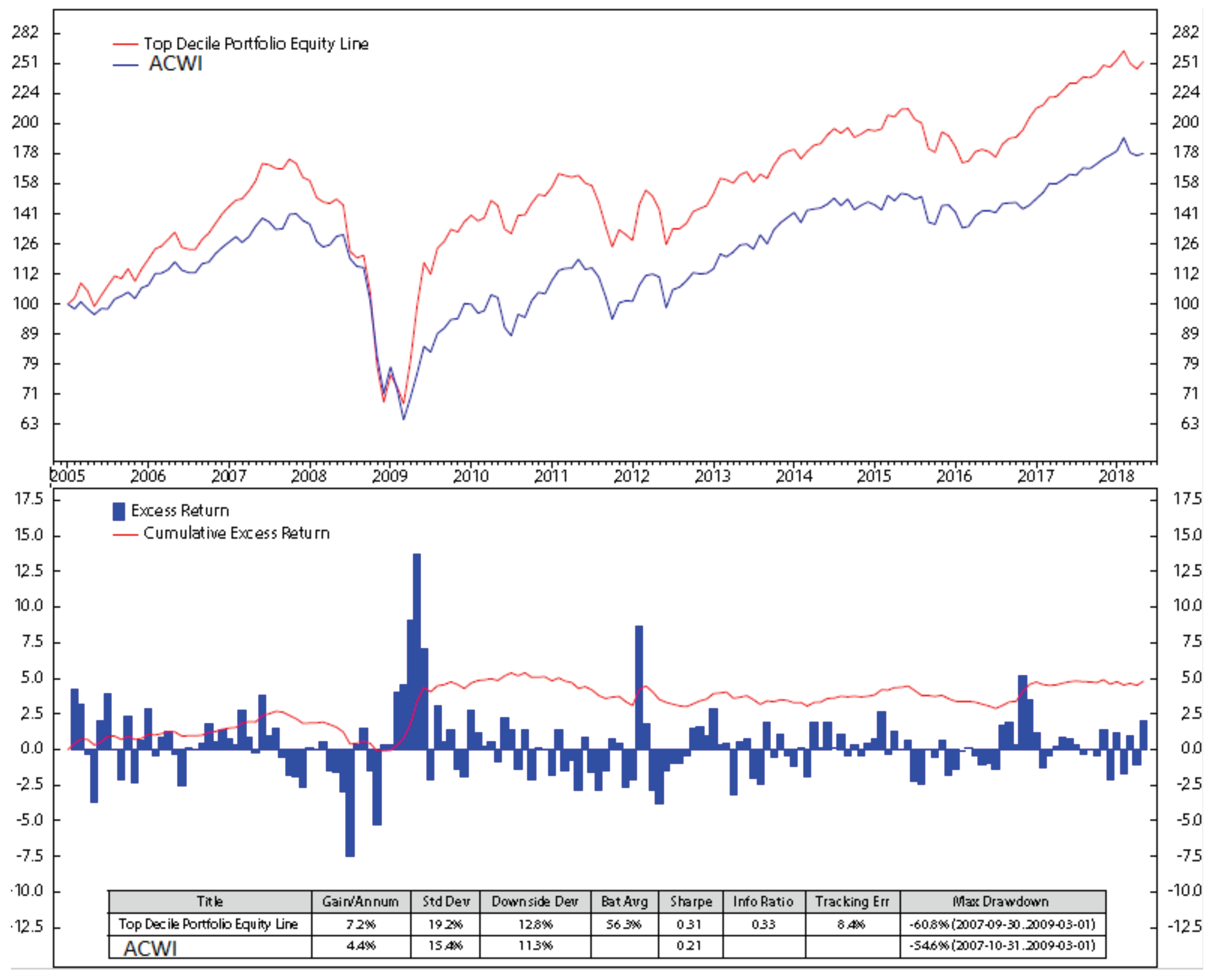
Figure 8 presents our stock selection portfolio (10% of the ACWI) based solely on the free cash flow/enterprise value (results based on other four factors, i.e., earning/price, sale/enterprise, long-term sale growth, and long-term earning per share growth are shown in Figure A7, Figure A8, Figure A9 and Figure A10 Appendix B). For each of the factors, we developed a global stock portfolio and compared it with the ACWI in terms of the monthly excess return (of our portfolio to the returns of the ACWI benchmark) and the accumulation of the excess returns. Figure 8 shows that with the initial investment of $100.00 in January 2005, our portfolio based on the ranking of the stock’s free cash flow/enterprise value got the value of $251.00 in September 2017, about 41% higher than the value of $178.00 of ACWI.
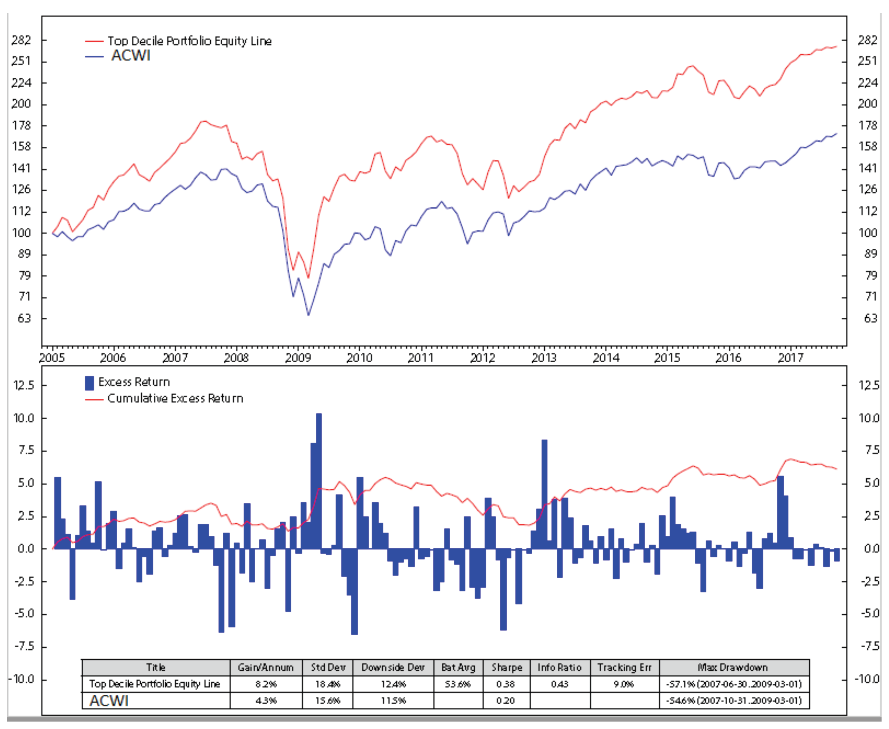
Among the single-factor models, the portfolio based on the sale/enterprise (see Figure A8) is the best with annual return of 8.2% (that of ACWI is 4.3%). The cumulative monthly excess return of this model is about 6% (compare to ACWI). On the other hand, the model based on the long-term earning per share growth in Figure A10 is the worst, performing just a little bit better than ACWI with the excess return of less than 1%.
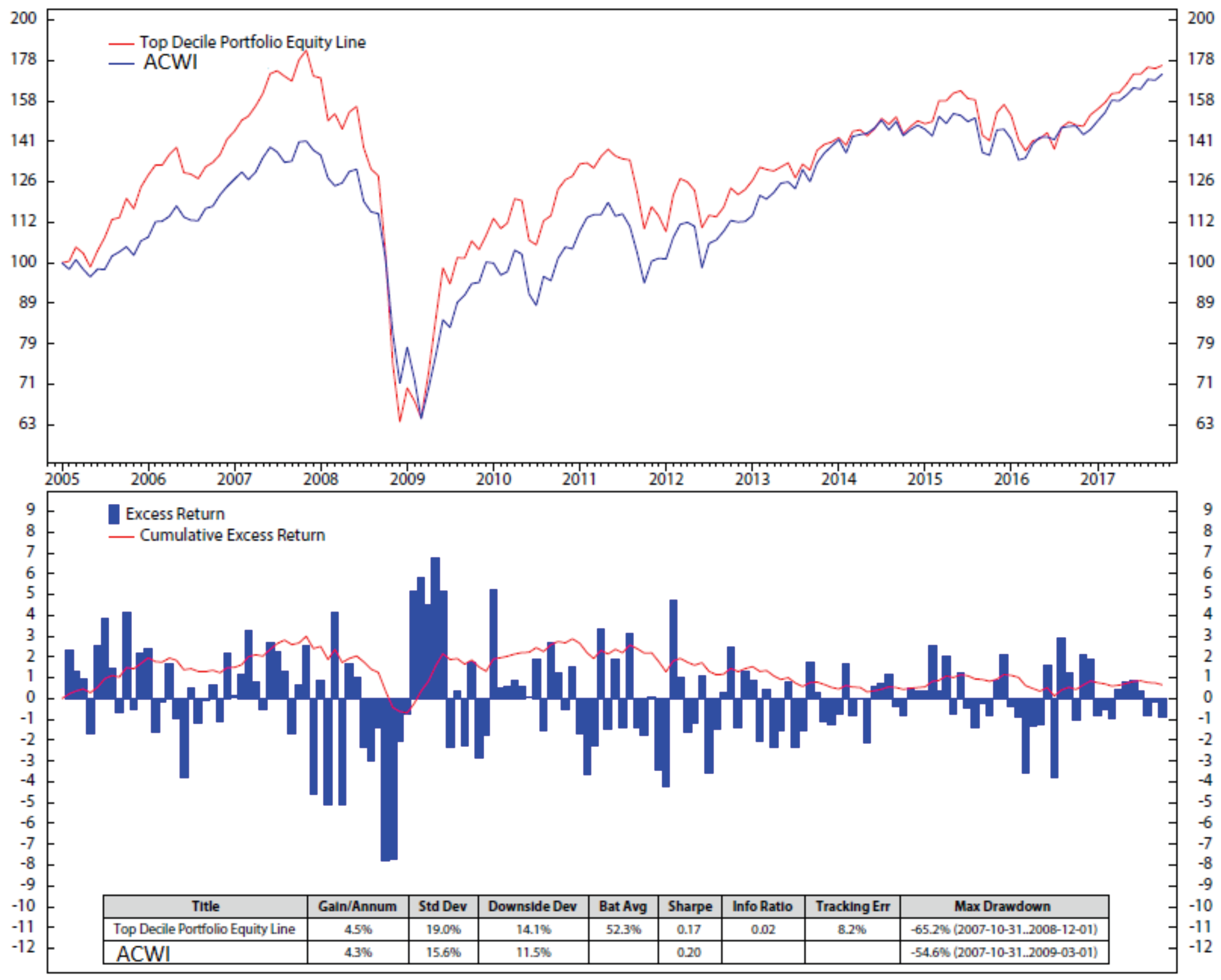
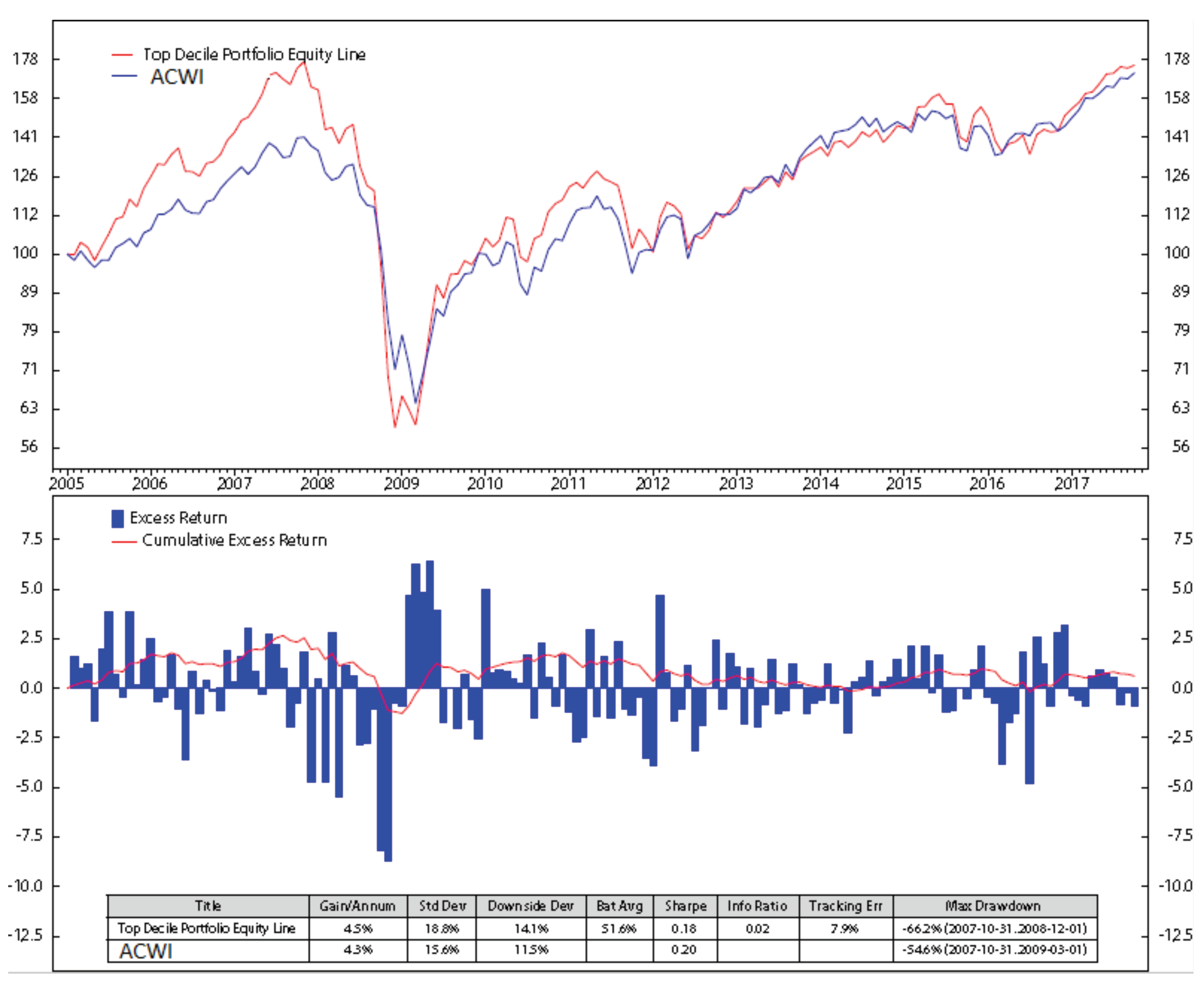
Figure 9 shows the performance of a stock selection portfolio based on the equal weight method (the weight of each factor is 20%), and the benchmark ACWI. This model yields an annual gain of 4.5% while that of ACWI is 4.3%. Although the gain of the equal-weighted portfolio is slightly higher than ACWI, it is also higher in risk compared to ACWI, as its Sharpe ratio is lower than that of ACWI.
Overall, our weighted model (using HMM) outperforms the equal-weighted model shown in Figure 9 and all of the single factor models shown in Appendix B. With the annual return of 9.4%, the excess return of 7.75%, and the Sharpe ratio of 0.44 during the testing period from January 2005 to September 2017 (as shown in Figure 7), the HMM model stands out from other investigated models as an efficient strategy for stock trading.
7. Conclusions
We have developed a multi-step procedure for using the unsupervised machine learning HMM in global stock selections. Given the past data, the stock score in each month is calculated using five stock factors, including free cash flow/enterprise value, earnings/price, sales/enterprise, long-term sales growth, and long-term earning per share growth. Then, the regimes of the six global economic indicators are predicted using HMM. The performances of each stock factor are analyzed for calculating its weighted score. Finally, we chose 10% of the global stocks with the highest weighted scores for our monthly trading portfolio. Our global stock trading based on HMM outperformed the trading portfolios based on the whole stocks in ACWI, the single stock factor, or the equal-weighted method of the five stock factors. In the time period from January 2005 to September 2017, the approximated returns of our portfolio is 210%, while the return of the equal-weighted method is almost equal to the return of the ACWI, which is 70%. The highest and lowest returns of the trading based on a single stock’s factor are approximated 180% (Figure A8) and 70% (Figure A10), respectively. In summary, the unsupervised ML HMM for global stock trading yielded great returns compared to those of the whole ACWI.
The successes of using HMM in global stock trading in this paper and the S&P 500 trading in our previous paper Nguyen and Nguyen (2015) proved that HMM is a great promised model for stock traders both locally and globally. We expanded the model to select stocks from a pool of about 500 stocks in the S&P 500 Nguyen and Nguyen (2015) to a pool of about more than 2500 stocks in AWCI. Analyzing the big pool of stocks is time consuming. Thus, in future works, we would like to use a simple model such as the moving average model to skim the pool first, then use HMM to do more complicated analysis for final stock selections. By doing that, we can work with high frequency trading, such as hourly or daily tradings.
Author Contributions
Conceptualization, N.N. and D.N.; methodology D.N.; software, D.N.; validation, N.N. and D.N.; formal analysis, D.N.; investigation, N.N.; data curation, D.N. writing—original draft preparation, N.N.; writing—review and editing, N.N.; visualization, N.N. and D.N. All authors have read and agreed to the published version of the manuscript.
Funding
This research received no external funding.
Conflicts of Interest
The authors declare no conflict of interest.
Appendix A. Regime Detection Using HMM
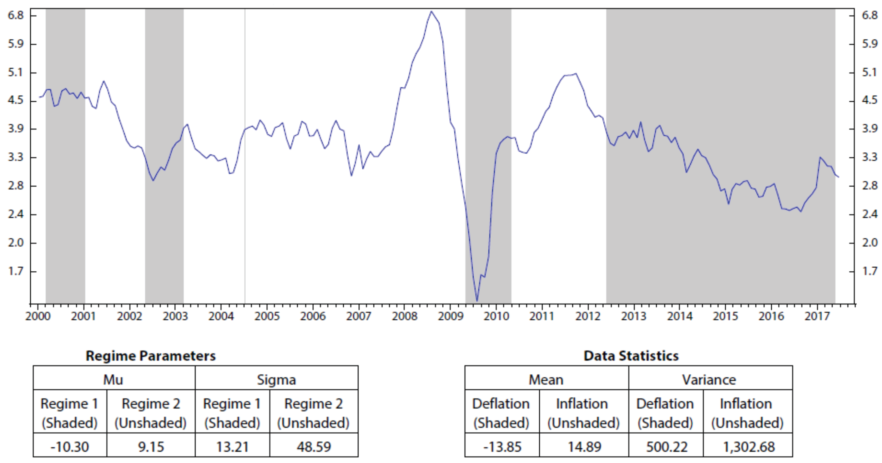
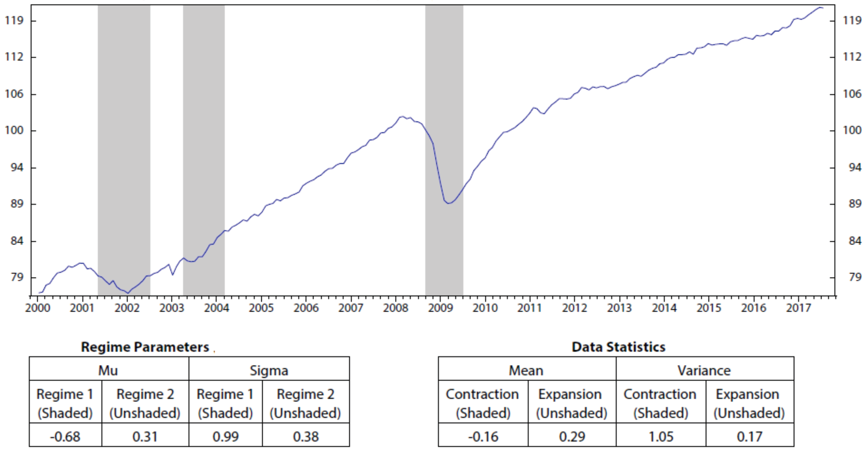
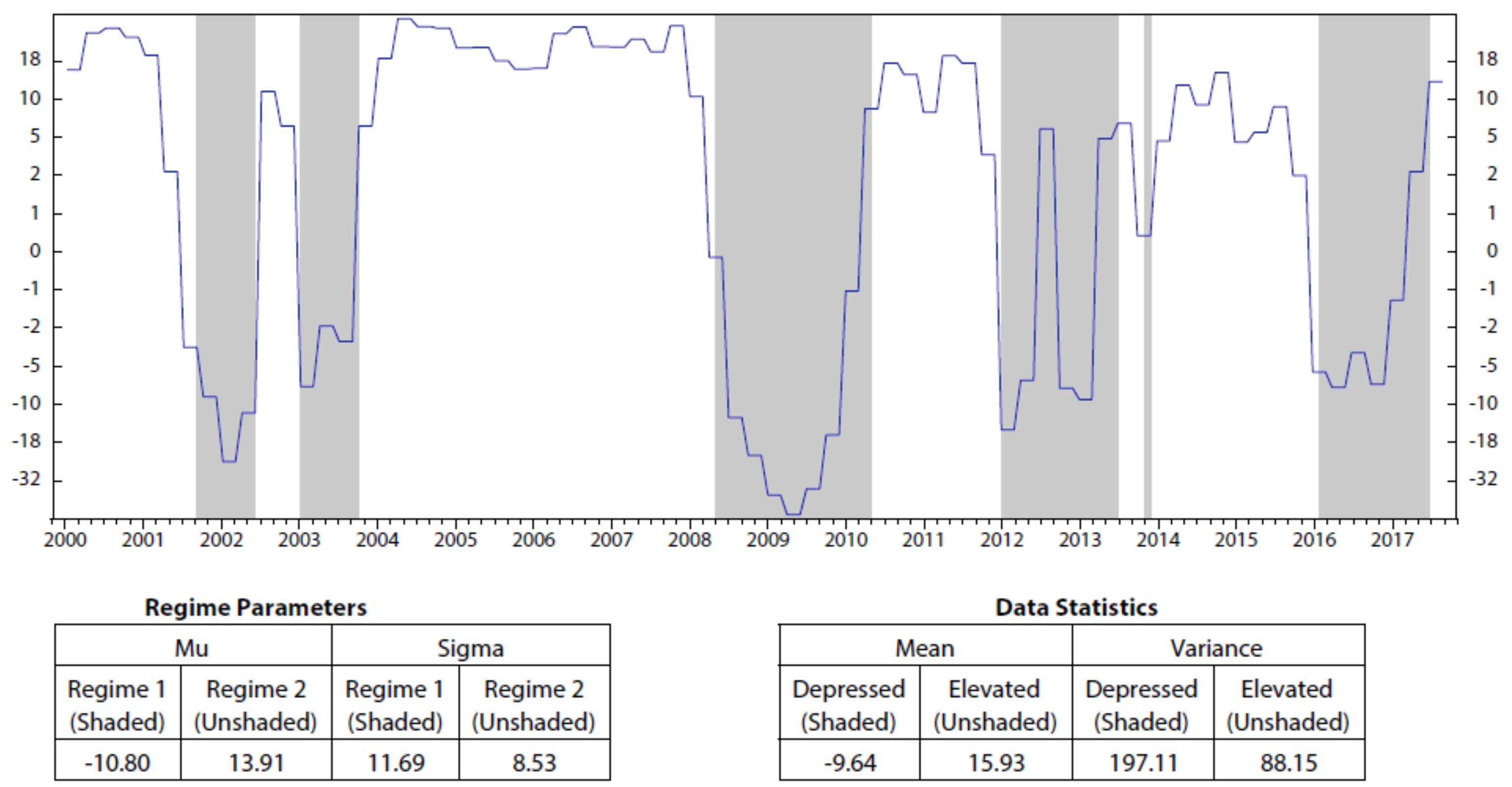
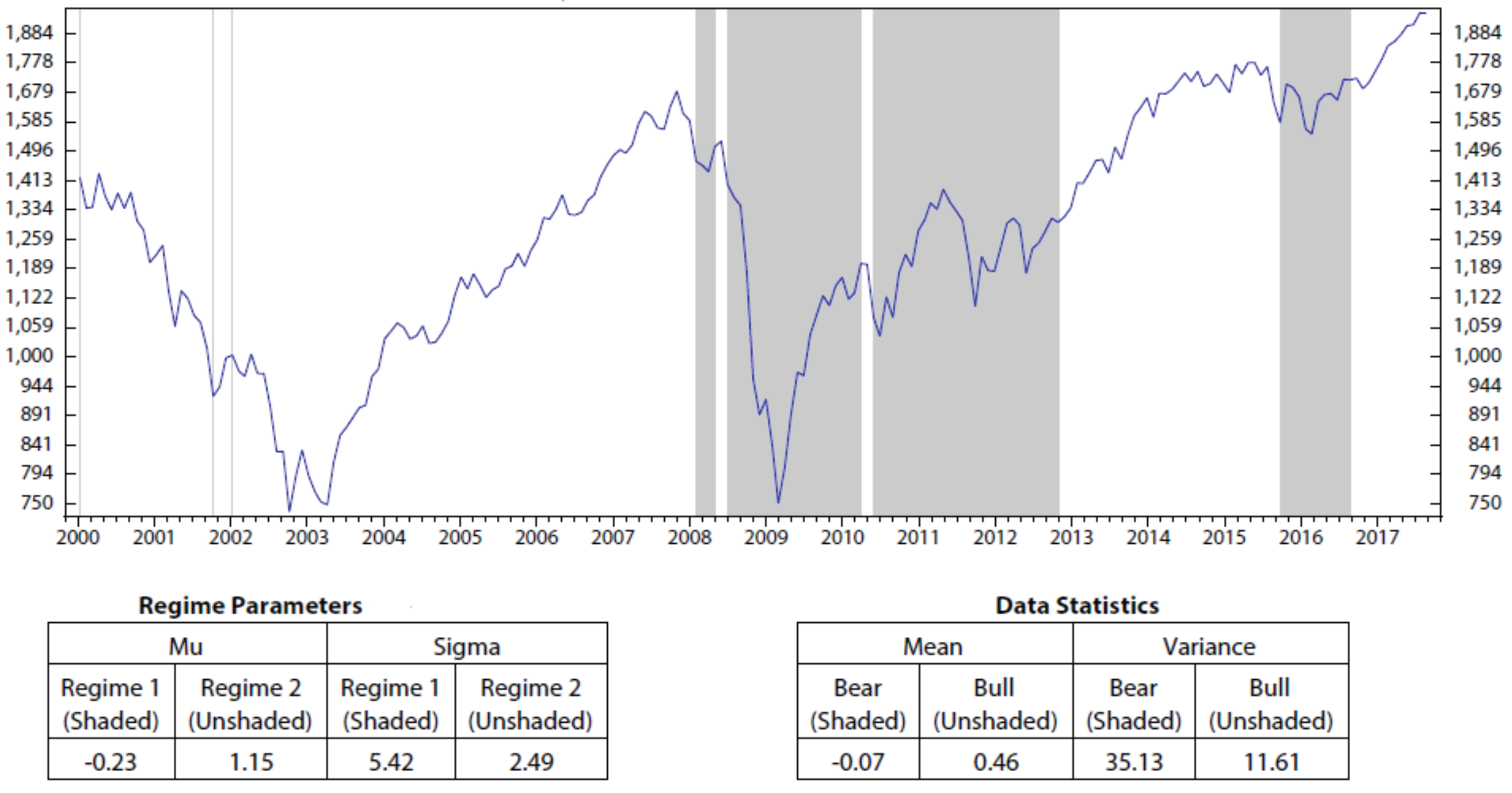
The regime prediction of using HMM for six stock factors are shown in Figure A1, Figure A2, Figure A3, Figure A4, Figure A5 and Figure A6. There are two tables below each of the figures, the left one presents the means and standard deviations of the two regimes, and the right one displays the mean and standard deviations of the returns of the observation data.
Figure A1.
The world inflation and its regimes detected using HMM for monthly data from 31 December 1999 to 31 August 2017. Regime 1 and regime 2 represent deflation and inflation periods, respectively.
Figure A1.
The world inflation and its regimes detected using HMM for monthly data from 31 December 1999 to 31 August 2017. Regime 1 and regime 2 represent deflation and inflation periods, respectively.

Figure A2.
The world production and its regimes detected using HMM for monthly data from 31 December 1999 to 31 August 2017. Regime 1 and regime 2 represent contraction and expansion periods, respectively.
Figure A2.
The world production and its regimes detected using HMM for monthly data from 31 December 1999 to 31 August 2017. Regime 1 and regime 2 represent contraction and expansion periods, respectively.

Figure A3.
The world sentiment and its regimes detected using HMM for monthly data from 31 December 1999 to 31 August 2017. Regime 1 and regime 2 correspond to the depressed and elevated periods of the world sentiment, respectively.
Figure A3.
The world sentiment and its regimes detected using HMM for monthly data from 31 December 1999 to 31 August 2017. Regime 1 and regime 2 correspond to the depressed and elevated periods of the world sentiment, respectively.

Figure A4.
The MSCI World index and its regimes detected using HMM for monthly data from 31 December 1999 to 31 August 2017. Regime 1 and regime 2 correspond to the Bear and Bull markets, respectively.
Figure A4.
The MSCI World index and its regimes detected using HMM for monthly data from 31 December 1999 to 31 August 2017. Regime 1 and regime 2 correspond to the Bear and Bull markets, respectively.

Figure A5.
The world debt and its regimes detected using HMM for monthly data from 31 December 1999 to 31 August 2017. Regime 1 and regime 2 represent the low and high periods of the world debt, respectively.
Figure A5.
The world debt and its regimes detected using HMM for monthly data from 31 December 1999 to 31 August 2017. Regime 1 and regime 2 represent the low and high periods of the world debt, respectively.

Figure A6.
The world inflation expectation and its regimes detected using HMM for monthly data from 31 December 1999 to 31 August 2017. Regime 1 and regime 2 represent the low and high periods of the world inflation expectation, respectively.
Figure A6.
The world inflation expectation and its regimes detected using HMM for monthly data from 31 December 1999 to 31 August 2017. Regime 1 and regime 2 represent the low and high periods of the world inflation expectation, respectively.

Appendix B. Stock Portfolio Performances
Figure A7, Figure A8, Figure A9 and Figure A10 present our portfolio performances base on different stock’s factor compare to the ACWI.
Figure A7.
Global stock selection from January 2005 to September 2017 based on stock earning/price factor.
Figure A7.
Global stock selection from January 2005 to September 2017 based on stock earning/price factor.

Figure A8.
Global stock selection from January 2005 to September 2017 based on stock sales/enterprise factor.
Figure A8.
Global stock selection from January 2005 to September 2017 based on stock sales/enterprise factor.

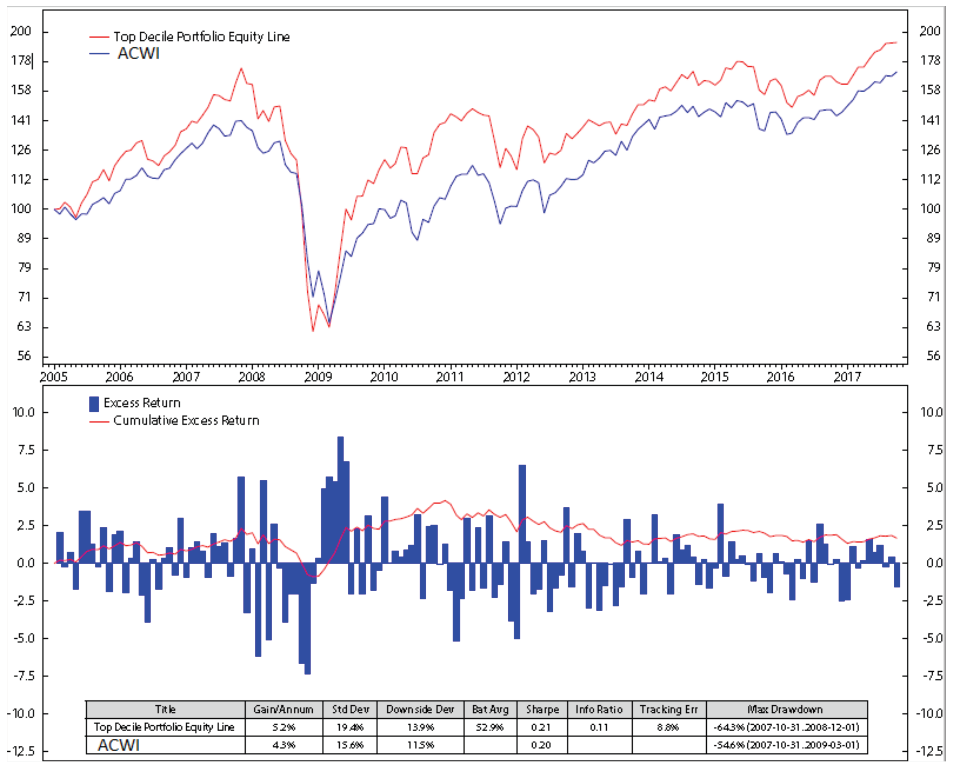
Figure A9.
Global stock selection from January 2005 to September 2017 based on stock long-term sales growth factor.
Figure A9.
Global stock selection from January 2005 to September 2017 based on stock long-term sales growth factor.

Figure A10.
Global stock selection from January 2005 to September 2017 based on stock long-term earning per share growth factor.
Figure A10.
Global stock selection from January 2005 to September 2017 based on stock long-term earning per share growth factor.

References
- Alloway, T. 2019. JPMorgan Creates ’Volfefe’ Index to Track Trump Tweet Impact. Bloomberg. Available online: https://www.bloomberg.com/news/articles/2019-09-09/jpmorgan-creates-volfefe-index-to-track-trump-tweet-impact (accessed on 9 September 2019).
- Andriosopoulos, Dimitris, Michalis Doumpos, Panos M. Pardalos, and Constantin Zopounidis. 2019. Computational approaches and data analytics in financial services: A literature review. Journal of the Operational Research Society 70: 1–19. [Google Scholar] [CrossRef]
- Ball, Philip. 2013. Counting Google searches predicts market movements. Natute News. [Google Scholar] [CrossRef]
- Baum, Leonard, and Ted Petrie. 1966. Statistical inference for probabilistic functions of finite state Markov chains. Institute of Mathematical Statistics 37: 1554–63. [Google Scholar] [CrossRef]
- Baum, Leonard, Ted Petrie, George Soules, and Norman Weiss. 1970. A maximization technique occurring in the statistical analysis of probabilistic functions of Markov chains. Annals of Mathematical Statistics 41: 164–71. [Google Scholar] [CrossRef]
- Brown, Frank K. 1998. Chapter 35—Chemoinformatics: What is it and How does it Impact Drug Discovery. In Annual Reports in Medicinal Chemistry. Cambridge: Academic Press, vol. 33, pp. 375–84. [Google Scholar]
- Bunke, H., Markus Roth, and Ernst Günter Schukat-Talamazzini. 1995. Off-line cursive handwriting recognition using hidden markov models. Pattern Recognit. 28: 1399–1413. [Google Scholar] [CrossRef]
- de Prado, Marcos Lopez. 2018. Advances in Financial Machine Learning, 1st ed. Hoboken: Wiley. [Google Scholar]
- Engel, Thomas. 2006. Basic Overview of Chemoinformatics. Journal of Chemical Information and Modeling 46: 2267–77. [Google Scholar] [CrossRef] [PubMed]
- Fan, Alan, and Marimuthu Palaniswami. 2001. Stock selection using support vector machines. Paper presented at the International Joint Conference on Neural Networks, Washington, DC, USA, July 15–19; vol. 3, pp. 1793–98. [Google Scholar]
- Graham, Benjamin. 2003. The Intelligent Investor, revised ed. New York: HarperCollins. [Google Scholar]
- Hamilton, James. 1989. A New Approach to the Economic Analysis of Nonstationary Time Series and the Business Cycle. Econometrica 57: 357–84. [Google Scholar] [CrossRef]
- Hassan, Rafiul, and Baikunth Nath. 2005. Stock Market Forecasting Using Hidden Markov Model: A New Approach. Paper presented at 5th International Conference on Intelligent Systems Design and Applications, Wroclaw, Poland, September 8–10. [Google Scholar]
- Hondroyiannis, George, and Evangelia Papapetrou. 2001. Macroeconomic influences on the stock market. Journal of Economics and Finance 25: 33–49. [Google Scholar] [CrossRef]
- Huan, Tran Doan, Arun Mannodi-Kanakkithodi, and Rampi Ramprasad. 2015. Accelerated materials property predictions and design using motif-based fingerprints. Physical Review B 92: 014106. [Google Scholar] [CrossRef] [Green Version]
- Huang, Chien-Feng. 2012. A hybrid stock selection model using genetic algorithms and support vector regression. Applied Soft Computing 12: 807–18. [Google Scholar] [CrossRef]
- Idvall, Patrik, and Conny Jonsso. 2008. Algorithmic Trading: Hidden Markov Models on Foreign Exchange Data. Master’s Dissertation, Linköping University, Linköping, Sweden. [Google Scholar]
- Kavitha, G., A. Udhayakumar, and D. Nagarajan. 2013. Stock Market Trend Analysis Using Hidden Markov Models. arXiv arXiv:arXiv:1311.4771. [Google Scholar]
- Khan, Jawad, and Imran Khan. 2018. The Impact of Macroeconomic Variables on Stock Prices: A Case Study of Karachi Stock Exchange. Journal of Economics and Sustainable Development 9: 2222–55. [Google Scholar] [CrossRef]
- Kim, Chiho, Anand Chandrasekaran, Tran Doan Huan, Deya Das, and Rampi Ramprasad. 2018. Polymer Genome: A Data-Powered Polymer Informatics Platform for Property Predictions. Journal of Physical Chemistry C 122: 17575–85. [Google Scholar] [CrossRef]
- Kritzman, Mark, Sébastien Page, and David Turkington. 2012. Regime Shifts: Implications for Dynamic Strategies. Financial Analysts Journal 68: 3. [Google Scholar] [CrossRef]
- Lajos, Jaroslav. 2011. Computer Modeling Using Hidden Markov Model Approach Applied to the Financial Markets. Ph.D. Dissertation, Oklahoma State University, Stillwater, OK, USA. [Google Scholar]
- Levinson, S., L. R. Rabiner, and M. M. Sondhi. 1983. An introduction to the application of the theory of probabilistic functions of Markov process to automatic speech recognition. Bell System Technical Journal 62: 1035–74. [Google Scholar] [CrossRef]
- Li, Na, and Matthew Stephens. 2003. Modeling Linkage Disequilibrium and Identifying Recombination Hotspots Using Single-Nucleotide Polymorphism Data. Genetics 165: 2213–33. [Google Scholar] [PubMed]
- Li, Xiaolin, Marc Parizeau, and Réjean Plamondon. 2000. Training Hidden Markov Models with Multiple Observations—A Combinatorial Method. IEEE Transactions on PAMI 22: 371–77. [Google Scholar]
- Liu, Guang, and Xiaojie Wang. 2019. A new metric for individual stock trend prediction. Engineering Applications of Artificial Intelligence 82: 1–12. [Google Scholar] [CrossRef]
- Liu, Yi-Cheng, and I-Cheng Yeh. 2017. Using mixture design and neural networks to build stock selection decision support systems. Neural Computing and Applications 28: 521–535. [Google Scholar] [CrossRef]
- Humpe, Andreas, and Peter Macmillan. 2009. Can macroeconomic variables explain long-term stock market movements? A comparison of the US and Japan. Applied Financial Economics 19: 111–19. [Google Scholar] [CrossRef]
- Mamon, Rogemar S., and Robert J. Elliott, eds. 2007. Hidden Markov Models in Finance. New York: Springer, vol. 104. [Google Scholar]
- Markowitz, Harry. 1952. Porfolio selection. Journal of Finance 7: 77–91. [Google Scholar]
- Nenortaite, Jovita, and Rimvydas Simutis. 2004. Stocks’ Trading System Based on the Particle Swarm Optimization Algorithm. In Computational Science—ICCS 2004. Edited by M. Bubak, G. D. van Albada, P. M. A. Sloot and J. Dongarra. Poland: Springer, pp. 843–50. [Google Scholar]
- Nguyen, Nguyet, and Dung Nguyen. 2015. Hidden Markov Model for Stock Selection. Risks 3: 455–73. [Google Scholar] [CrossRef] [Green Version]
- Nguyen, Nguyet, Dung Nguyen, and Thomas Wakefield. 2018. Using the Hidden Markov Model to Improve the Hull-White Model for Short Rate. International Journal of Trade, Economics and Finance 9: 54–59. [Google Scholar] [CrossRef]
- Nguyen, Nguyet. 2017a. Hidden Markov Model for Portfolio Management with Mortgage-Backed Securities Exchange-Traded Fund. Technical Report. Schaumburg: Society of Actuaries. [Google Scholar]
- Nguyen, Nguyet. 2017b. An Analysis and Implementation of the Hidden Markov Model to Technology Stock Prediction. Risks 5: 62. [Google Scholar] [CrossRef] [Green Version]
- Nijam, Habeeb Mohamed, Smm Ismail, and Amm Musthafa. 2015. The Impact of Macro-Economic Variables on Stock Market Performance; Evidence from Sri Lanka. Journal of Emerging Trends in Economics and Management Sciences 6: 151–57. [Google Scholar]
- Pardo, Bryan, and William Peter Birmingham. 2005. Modeling form for on-line following of musical performances. Paper Presented at 20th National Conference on Artificial Intelligence, Pittsburgh, PA, USA, 9–13 July; pp. 1018–23. [Google Scholar]
- Preis, Tobias, Helen Susannah Moat, and Stanley H. Eugene. 2013. Quantifying Trading Behavior in Financial Markets Using Google Trends. Scientific Reports 3: 1684. [Google Scholar] [CrossRef] [Green Version]
- Rabiner, L. R., and B. H. Juang. 1992. Hidden Markov Models for Speech Recognition—Strengths and Limitations. In Speech Recognition and Understanding. Edited by P. Laface and R. De Mori. Berlin: Springer, pp. 3–29. [Google Scholar]
- Sanborn, B., D. Nguyen, and T. Nguyen. 2017. Global Factor-Based Investing—Opportunities, Risks, and Implementation. Technical Report: Ned Davis Research-NDR Explorer-Insights. [Google Scholar]
- Satish, L., and B. I. Gururaj. 1993. Use of hidden Markov models for partial discharge pattern classification. IEEE Transactions on Electrical Insulation 28: 172–82. [Google Scholar] [CrossRef]
- Thawornwong, Suraphan, and David Enke. 2004. Forecasting Stock Returns with Artificial Neural Networks. In Neural Networks in Business Forecasting. Edited by G. Peter Zhang. Hershey: IRM Press. [Google Scholar]
- Yoon, Byung-Jun. 2009. Hidden Markov Models and their Applications in Biological Sequence Analysis. Current Genomics 10: 402–15. [Google Scholar] [CrossRef] [Green Version]
- Yu, Lean, Lunchao Hu, and Ling Tang. 2016. Stock Selection with a Novel Sigmoid-Based Mixed Discrete-Continuous Differential Evolution Algorithm. IEEE Transactions on Knowledge and Data Engineering 28: 1891–904. [Google Scholar] [CrossRef]
Figure 1.
Hidden Markov model (HMM) with two states.

Figure 2.
HMM process.

Figure 3.
Distribution of All country world index (ACWI) by (a) financial companies’ locations, (b) market cap, and (c) sectors as of August 2017.
Figure 3.
Distribution of All country world index (ACWI) by (a) financial companies’ locations, (b) market cap, and (c) sectors as of August 2017.

Figure 4.
The correlation coefficients of the global economic indicators.

Figure 5.
Performances of six global economic indicators from 2004 to 2017.

Figure 6.
Calculated weights of five global stock factors from January 2005 to September 2017.

Figure 7.
(log scale) Monthly global stock selection portfolio performances using HMM and the benchmark ACWI from January 2005 to September 2017. The stock prices were scaled to $100.00 at the beginning of the stock selection process (January 2005). The bottom table summarizes the performances of the portfolio, including annual gain (gain/annum), standard deviation, downside deviation, batting average, Sharpe ratio, information ratio (info ratio), tracking error, and the maximum drawdown of the data.

Figure 8.
Global stock selection from January 2005 to September 2017 based on stock free cash flow/enterprise factor. The stock prices were scaled to $100.00 at the beginning of the stock selection process (January 2005).
Figure 8.
Global stock selection from January 2005 to September 2017 based on stock free cash flow/enterprise factor. The stock prices were scaled to $100.00 at the beginning of the stock selection process (January 2005).

Figure 9.
Top decile of valuation composite performance using the equally-weighted model from January 2005 to September 2017. The stock prices were scaled to $100.00 at the beginning of the stock selection process (January 2005).
Figure 9.
Top decile of valuation composite performance using the equally-weighted model from January 2005 to September 2017. The stock prices were scaled to $100.00 at the beginning of the stock selection process (January 2005).


Table 1.
Basic concepts of a hidden Markov model.
| Variable | Notation |
|---|---|
| Length of observation data | T |
| Number of states | N |
| Number of symbols per state | M |
| Observation sequence | |
| Hidden state sequence | |
| Possible values of each state | |
| Possible symbols per state | |
| Transition matrix | , where |
| Vector of initial probability of being in state (regime) at time | , where |
| Observation probability matrix | , where and |
Table 2.
Global economic indicators and sources used in this work.
| Indicator | Name | Source | Data Used |
|---|---|---|---|
| Inflation | Consumer price index | International Monetary Fund | Yearly change |
| Production | Industrial production | Haver Analytics | Monthly change |
| Sentiment | Economic climate index | Ifo Institute for Economic Research | Original series |
| Market | MSCI world index | Morgan Stanley, Capital International | Monthly change |
| Debt | Public and private non-financial debt | Bank for International Settlements | Monthly change |
| Inflation expectation | Manufacturing purchasing managers’ index | Haver Analytics | Yearly change |
Table 3.
Definition of the stock factors.
| Stock Factor | Definition and Meaning |
|---|---|
| Free cash flow/enterprise value | Operating cash flow subtracted by the sum of cash dividends plus capital expenditures divided by the market value of equity plus debt. |
| Earning/price | Earnings accumulated over the trailing twelve months of the stock divided by the weekend price. A higher number indicates a greater value for each unit of earnings, which tends to drive a higher stock return. |
| Sale/enterprise | Sales accumulated over the trailing twelve months of the stock divided by the market value of equity plus debt (enterprise value). A higher sale/enterprise value signifies that each unit of a stock’s value is used to generate more sales, which normally leads to higher stock return. |
| Long-term sale growth | The projected long-term growth rate of sales based on a five-year moving regression trend line. A high sale growth rate normally leads to a higher future returns. |
Publisher’s Note: MDPI stays neutral with regard to jurisdictional claims in published maps and institutional affiliations. |
© 2020 by the authors. Licensee MDPI, Basel, Switzerland. This article is an open access article distributed under the terms and conditions of the Creative Commons Attribution (CC BY) license (http://creativecommons.org/licenses/by/4.0/).
Share and Cite
MDPI and ACS Style
Nguyen, N.; Nguyen, D. Global Stock Selection with Hidden Markov Model. Risks 2021, 9, 9. https://0-doi-org.brum.beds.ac.uk/10.3390/risks9010009
AMA Style
Nguyen N, Nguyen D. Global Stock Selection with Hidden Markov Model. Risks. 2021; 9(1):9. https://0-doi-org.brum.beds.ac.uk/10.3390/risks9010009
Chicago/Turabian StyleNguyen, Nguyet, and Dung Nguyen. 2021. "Global Stock Selection with Hidden Markov Model" Risks 9, no. 1: 9. https://0-doi-org.brum.beds.ac.uk/10.3390/risks9010009
Note that from the first issue of 2016, this journal uses article numbers instead of page numbers. See further details here.