Bayesian Predictive Analysis of Natural Disaster Losses


Department of Mathematics, Towson University, Towson, MD 21252, USA
*
Author to whom correspondence should be addressed.
Risks 2021, 9(1), 12; https://0-doi-org.brum.beds.ac.uk/10.3390/risks9010012
Submission received: 20 November 2020
/
Revised: 16 December 2020
/
Accepted: 18 December 2020
/
Published: 2 January 2021
Abstract
:Different types of natural events hit the United States every year. The data of natural hazards from 1900 to 2016 in the US shows that there is an increasing trend in annul natural disaster losses after 1980. Climate change is recognized as one of the factors causing this trend, and predictive analysis of natural losses becomes important in loss prediction and risk prevention as this trend continues. In this paper, we convert natural disaster losses to the year 2016 dollars using yearly average Consumers Price Index (CPI), and conduct several tests to verify that the CPI adjusted amounts of loss from individual natural disasters are independent and identically distributed. Based on these test results, we use various model selection quantities to find the best model for the natural loss severity among three composite distributions, namely Exponential-Pareto, Inverse Gamma-Pareto, and Lognormal-Pareto. These composite distributions model piecewise small losses with high frequency and large losses with low frequency. Remarkably, we make the first attempt to derive analytical Bayesian estimate of the Lognormal-Pareto distribution based on the selected priors, and show that the Lognormal-Pareto distribution outperforms the other two composite distributions in modeling natural disaster losses. Important risk measures for natural disasters are thereafter derived and discussed.
1. Introduction
Different types of natural events hit the United States (US) every year. The east coast of the US suffers hurricanes, the middle of the US sees tornadoes, the west coast of the US endures earthquake, and the south of the US bears a variety of issues such as hurricane, wind, drought, and floods1. The data of the occurrence and damage of natural events from 1900 to present in the US, from the Emergency Events Database (EM-DAT)—International Disaster Database2, showed that every year’s natural disaster losses after 1980 have been increasing. Climate change is recognized as one of the contributors to this increasing natural losses. Injury, homelessness, displacement, and economic losses from natural events can have significant impact on populations and societies. Predictive analysis of future natural events is imperative to provide important information for prevention and remedy plans to reduce the human impact and economic losses from natural disasters.
Various research has attempted to model the frequencies and damages due to the natural events. Levi and Partrat (1991) analyzed hurricane losses between 1954 and 1986 in the US, and found that the amounts of losses were independent and identically distributed (i.i.d.) and independent of the frequencies of hurricanes. These assumptions are confirmed in our research, based on the EM-DAT natural disaster data from 1900 to 2016 after taking into account price inflations. The number of losses in different years is converted into 2016 dollars using the annual average Consumers Price Index (CPI)3. We found that both the numbers of natural events and the CPI adjusted total damages have been increasing over the time; however there is no visible trend in the individual CPI adjusted losses, which is consistent with the conclusion claimed by Levi and Partrat (1991).
To discover the distribution features of individual losses from natural disasters, we use the most recent 37 years of the CPI adjusted amounts of natural losses to investigate appropriate parametric distribution models for the amount of loss caused by individual natural event, i.e., natural loss severity. Levi and Partrat (1991) proposed to use lognormal distribution for the losses of natural events based on the hurricane data between 1954 and 1986 in the US. However, this distribution cannot describe the typical feature of the natural disaster losses, i.e., many small amounts of losses and occasional occurrence of huge amount of losses. Some researchers argued to use composite distributions to capture this recognized feature.
A composite distribution has a threshold for the support of the loss random variable, with the Pareto distribution usually used to model a large loss beyond the threshold amount and popular parametric continuous distributions used for a small amount of loss below the threshold. For example, Bakar et al. (2015) developed several Weibull distribution-based composite models for heavy tailed insurance loss data. In our paper, we compare the performance of three composite distributions, namely Exponential-Pareto (Exp-Pareto), Inverse Gamma-Pareto (IG-Pareto), and Lognormal-Pareto (LN-Pareto), and the corresponding three non-composite parametric models, based on the negative loglikelihood, the Akaike information criterion, and Bayesian information criterion. All the three model selection criteria show that the composite distributions fit the data better than the non-composite models.
We thereafter apply the three composite models to the data and select the best fitted composite model for the loss severity of natural events. For consistent model comparison, we make the first attempt to derive analytic Bayesian estimation of the LN-Pareto composite distribution, because Aminzadeh and Deng (2018, 2019) has analytically derived Bayesian estimators for Exp-Pareto and IG-Pareto. In addition, Bayesian method enables us to perform predictive analysis of future losses of natural disasters using the best fitted composite model.
Cooray and Cheng (2015) developed Bayesian estimators for the LN-Pareto composite model based on a Markov Chain Monte Carlo (MCMC) simulation algorithm. In our paper, we carefully select prior distributions for the LN-Pareto composite model and derive a closed form Bayesian estimators for the unknown parameters of the LN-Pareto distribution. The mean squared errors (MSE) of the Bayesian estimation method and the maximum likelihood (ML) estimation method show that Bayesian estimation method outperform the ML estimation method in estimating these three composite models.
The comparison results show that the LN-Pareto is the best among these three composite models for the loss severity of natural disasters. Various risk measures of natural event losses are thereafter presented based on the LN-Pareto distribution. Same risk measures based on the other two composite distributions of natural losses are also provided for comparison.
The remainder of this paper is organized as follows. Section 2 describes the natural disaster data and tests the assumption that individual loss amounts are independent and identically distributed. Section 3 introduces three composite distributions and compare these models with the corresponding non-composite models. Section 4 derives Bayesian estimators for the LN-Pareto composite distribution and demonstrates the performance of Bayesian estimation method versus the ML estimation method. Section 5 presents risk measures of the future natural disaster losses based on the LN-Pareto model and the other two composite distributions. The concluding remarks are given in Section 6.
2. Natural Losses in the US
2.1. The Data
The EM-DAT contains worldwide data on the occurrence and impact of natural events from 1900 to the present day. The database is compiled from various sources, including United Nation agencies, non-governmental organizations, insurance companies, research institutes and press agencies. There were a total of 258 natural events in the US from 1900 to 2016, among which 156 events happened between 1980 to 2016, accounting for 60% of the total events during this one third of the whole time period. This observation is consistent with the fact that Earth’s climate is changing faster than at any point in the history as a result of human activities.
We also look into the trend of the natural loss amounts from 1900 to 2016. To eliminate the effect of price inflation, we convert the amounts of losses in each year into the year 2016 dollars. Let be the annual average CPI in year t and be the CPI adjusted amount of losses in that year, then we have
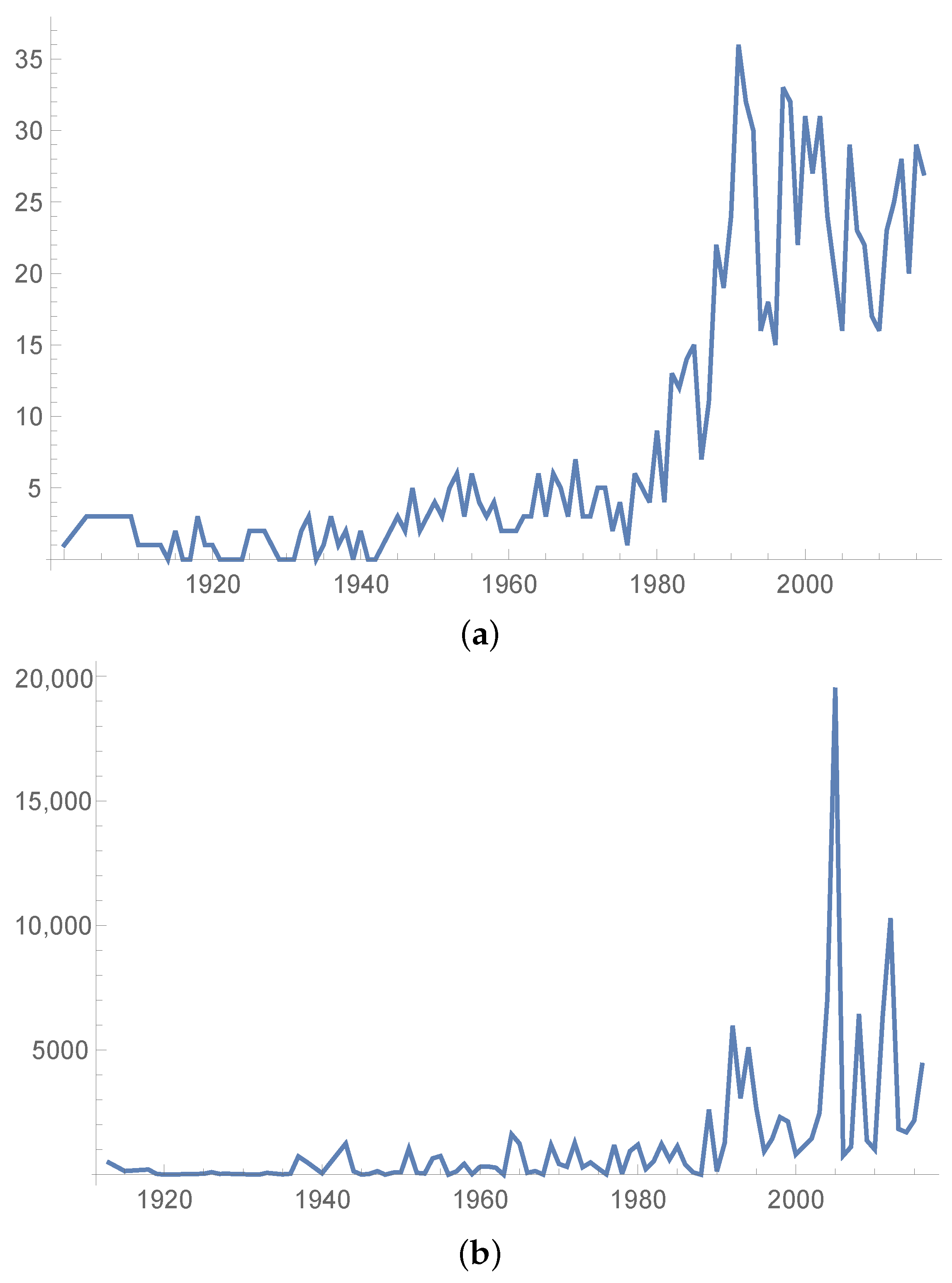
After price inflation effect being adjusted, the amount of losses during 1980 to 2016 accounts for 85.3% of the total losses. Figure 1 shows the yearly number of natural events and the CPI adjusted (in 2016 dollars) total damage costs from 1900 to 2016 in the US. We can see that both the number of natural events and the CPI adjust damage costs in each year have been increasing over these years, especially after 1980.
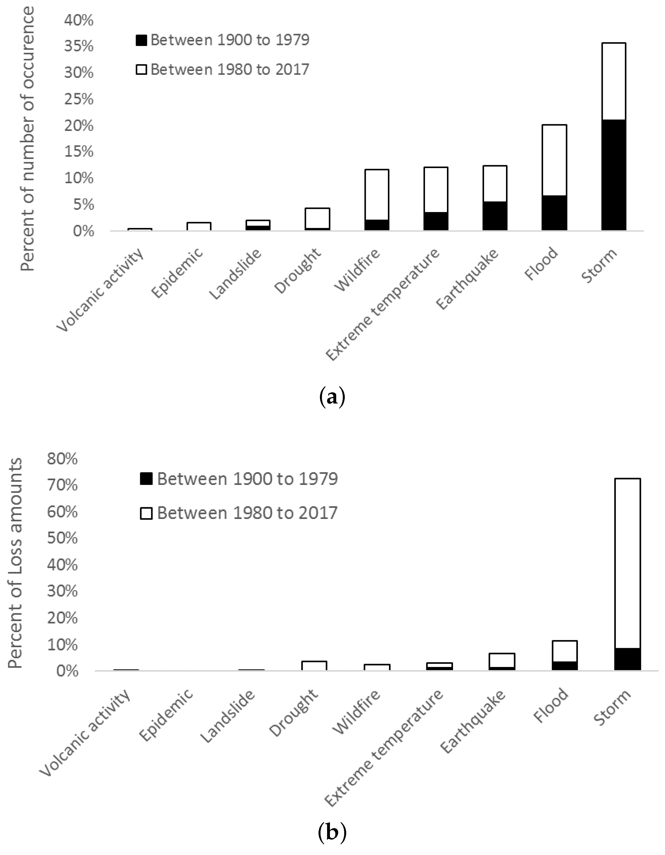
To demonstrate the change in both number and damage costs of natural events caused by human activities, we break down the data to be before and after 1980. Figure 2 displays the percentage of the number of occurrence to the total number of occurrence and the percentage of the CPI adjusted damage costs to the total losses by different time periods (before and after 1980) and by different types of natural disasters. The exact numbers for this figure are listed in Table A1 and Table A2 in Appendix A.
We can see that storms and floods account for most of natural events. The damage costs from natural events after 1980 account for the majority of the total costs, among which the damage costs caused by storms after 1980 account for more than half. In addition, these storm losses were caused by fewer storms after 1980 than before 1980, indicating higher average storm losses after 1980 than before 1980. However, this is not the case for other types of natural events.
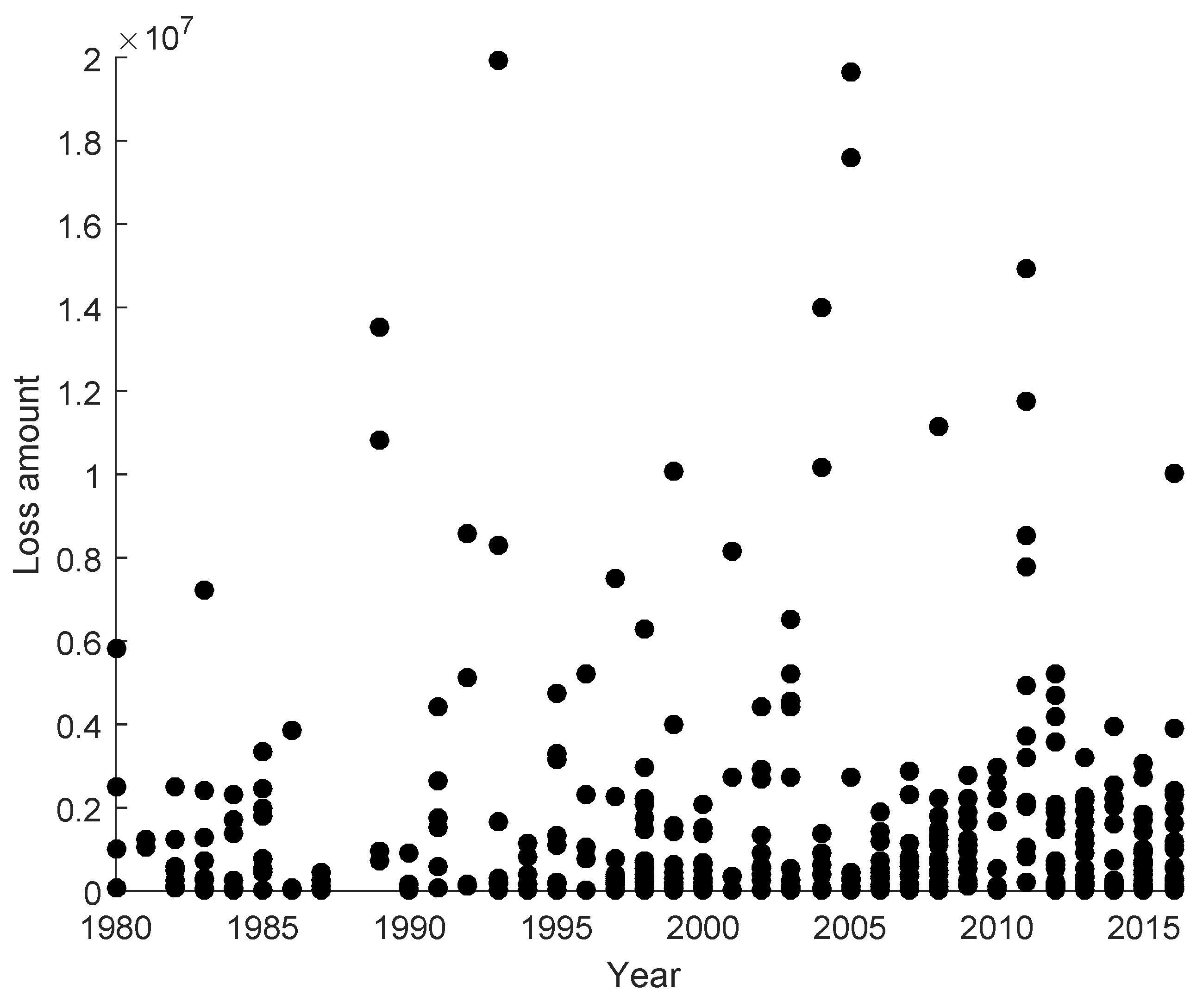
Although there is an obvious increasing trend in both the numbers and the total damage costs of natural events after 1980, it is not trivial to find out the pattern in the economic losses of individual natural events. Based on the aforementioned features of the natural loss data, we use the natural losses in the most recent 37 years from 1980 to 2016. There are a total number of 462 natural events in these 37 years, and only seven events caused economic loss above (in 2016 dollars). In Figure 3, we depict the scatter plot of those losses below , and we can see that there is no identified trend in individual natural disaster losses.
We are interested in how to appropriately model individual natural disaster losses. Motivated by this research question and the above observations, in this paper we aim to investigate the features of the severity of natural events, attempt to find appropriate loss severity models for natural disasters, and provide the predictive modeling of loss severity for risk management and insurance arrangement.
2.2. The i.i.d. Assumption for Loss Severity
Let the random variable N denote the number of occurrences per year and , for , be the severity random variable of the occurrence of natural events occurring in each year. The vector denotes the random vector of yearly loss severity. We use the natural disaster data between 1980 to 2016, and the random variable N has a sample size of 37. Table A3 in Appendix B lists the CPI adjusted individual natural damage losses in these 37 years. It can easily be seen that random variable N takes one of the values over the 37 years. One value of N is zero, because there was no record of natural events in year 1988. In all other years, there were at least two natural events every year. Therefore, there are 36 non-zero realizations of . The column in the matrix are the realizations of , i.e., the occurrence of natural disasters in each of 36 years.
Let be the sample size of the random variable . From Table A3 we also see that , the 1st severity random variable, has 36 non-zero values and therefore the sample size . The realization of is , which takes the value million in 2016 dollars. , the 28th severity random variable with and takes only one non-zero value millions in 2016 dollars, because there is only one year with 28 losses. The total number of the observation is .
We want to test the general assumption that are independent and identically distributed random variables. Since have small sample sizes, we group them together as one random variable . Applying the nonparametric methods, the Kendall Tau test and the Spearman test (see Gibbons and Chakraborti 2003), we test the independence assumption for as follows.
For , where , the null hypotheses and alternative hypotheses are
Let . The Kendall Tau statistic is
where
Let and be the rank of and among m observations respectively, for . The Spearman rho test statistic is
where and are the average of and respectively.
For , there are total of tests. We obtain 210 values of all the Kendall Tau test statistic and Spearman test statistic with the corresponding p-values. Table 1 lists the pairs of severity random variables with the null hypotheses being rejected at the significance level of 1%. All other pairs have non-significant test results and we fail to reject the null hypotheses at the significance level of 1%. Based on these test results, it is reasonable to assume that are independent.
Next, the Kruskal-Wallis test is used to verify the identical distribution assumption. The details of this test are introduced by Gibbons and Chakraborti (2003). Let be the cumulative distribution function of . In our Kruskal-Wallis test, the null hypotheses and alternative hypotheses are
There are a total of 462 observations. Sort all the 462 observations in an increasing order. If there are more than one observations with an identical value, then the median is assigned as the rank for these observations. Define to be the sum of the ranks of all the observations of , where . We have , and . It is clear that 106,854.
Under the null hypotheses, . Therefore, 88,334, …, and . The Kruskal-Wallis Statistic is
Asymptotically, has Chi-Square distribution with the degree of freedom 20, with the p-value 0.494. We fail to reject at the significance level 1%. Therefore, it is reasonable to assume that are identically distributed.
2.3. Non-Parametric Distribution of Loss Severity
Based on the test results, we can reasonably assume that the CPI adjusted natural disaster damage random variable is independent and identically distributed. Let X denote the CPI adjusted damage random variable with unknown distribution . The 462 individual damage losses are the realizations of the loss severity random variable X. As we explore an appropriate parametric distribution for the natural disaster loss severity, we first look at the non-parametric distribution of X, which is also called a data dependent distribution.
Let be the k unique loss values, and be the number of times the observations appears in the sample. Let be the number of observations greater than or equal to . The Nelson-Aalen estimator of the cumulative hazard rate function is
Therefore, and . The Kolmogorov -Smirnov (K-S) confidence band of unknown distribution can also be constructed based on the Nelson Aalen estimate of distribution . Define the K-S statistics by , where n is sample size. To form % conference band, we select a number d such that . Then, the lower band is and the upper band is . We set and the true unknown distribution of loss lies between and with 95% confidence.
The plots of , and is given in Panel (a) of Figure 4. We also display the histogram of the CPI adjusted severity of the natural events in Panel (b) of Figure 4. We can see that the histogram of the CPI adjusted severity of the natural event losses is both skewed and fat-tailed, which shows the typical feature that there are many small losses and a few very large losses.
3. Composite Models
We confirmed that the natural event severity data has the typical feature of high frequency of small losses and low frequency of large losses; while the traditional distributions such as the normal, exponential, inverse-gamma, and log-normal distributions, are not able to describe this feature. Some researchers have addressed this feature of insurance data by using composite models for insurance losses. The probability density function of a composite model consists of two distributions, namely probability density functions and . The general composite model has the probability density function as follows.
where c is a normalized constant and is the parameter that represents the threshold of the supports for the two distributions. In order to make the composite density function smooth, it is usually assumed that the pdf is continuous and differentiable at , that is and
3.1. Three Composite Distributions
Cooray and Ananda (2005) introduced a two-parameter continuous and differentiable composite LN-Pareto model, which is a two-parameter lognormal density up to an unknown threshold value and a two-parameter Pareto density for the rest of the model. The resulting density is similar in shape to a lognormal density with the tail behavior quite similar to a Pareto density. They applied the proposed composite model to a fire insurance data to show the importance of the proposed composite LN-Pareto distribution in describing insurance claim data.
Motivated by Cooray and Ananda (2005), Teodorescu and Vernic (2006) introduced a composite Exp-Pareto distribution, which is an exponential density up to an unknown threshold value and a two parameter Pareto density for the rest of the model. The model is reduced to a one-parameter distribution after satisfying the continuous and differentiable condition. Aminzadeh and Deng (2019) proposed an IG-Pareto composite model. Under the general assumption of smoothness and continuity, the IG-Pareto model is reduced to be a one parameter model. Let be the cumulative distribution function (cdf) of the standard normal distribution. Table 2 summarizes the distribution density function of Exp-Pareto, LN-Pareto, and IG-Pareto composite models, and Figure 5 plots three distribution functions with various parameter values.
We can see that the Nelson Aalen estimate of the unknown distribution of the natural disaster severity loss random variable is quite similar to the distributions of three composite models. This indicates that composite models might be able to describe the features of the natural disaster damage losses. In the next section, we will compare the performance of these three composite distributions in modeling the natural disaster loss severity based on standard model comparison and selection criteria.
3.2. Model Selection for Loss Severity
The maximum likelihood estimators for the unknown parameters of the Exp-Pareto, IG-Pareto, and Lognormal-Pareto composite models have been derived by Teodorescu and Vernic (2006), Aminzadeh and Deng (2019), and Cooray and Ananda (2005) respectively. We know that the parameter is the unknown threshold value dividing the domain of the two distributions of a composite model, and the maximum likelihood functions changes when the value of changes; therefore, a grid search method has to be used to find the ML estimates. The grid search algorithm can be briefly summarized as follows.
- 1.
- Sort the sample of the natural disaster damage losses in an increasing order, i.e., , where n is the sample size. Let be the size of the partial sample of the first losses . Start from .
- 2.
- Compute the maximum likelihood estimates and as in Table 3 for the given . If is in between , we found ; otherwise, increase by 1.
- 3.
- Repeat Step 2 for till . The ML estimates of the parameters are found based on the correct .
In our research, Mathematica software is used to code the algorithm. Table 3 lists the ML estimates of three composite distributions.
Based on the ML estimates, we use the negative log-likelihood (NLL) value, the Akaike’s Information Criterion (AIC), the Bayesian Information Criterion (BIC) goodness-of-fit measures to compare the appropriateness of these three composite models in modeling the natural disaster severity.
can be used to compare models with the same number of parameters. It is equivalent to the maximum value of the likelihood function and defined as
where is the vector of unknown parameters. The smaller the NLL value, the larger the value of the likelihood function, and the better the fitted model.
AIC was defined by Akaike (1973) as
where q is the number of unknown parameters. The smaller the AIC value, the better the fitted model. The first term will decrease when the number of unknown parameters increases and is offset by the value of , indicating a trade-off between the goodness-of-fit and the number of parameters.
was developed by Schwarz (1978) and defined as
where n is sample size and q is the number of parameters. penalizes a large number of parameters and a big size of sample. The smaller the BIC, the better the fitted model. Interested readers are referred to Burnham and Anderson (2002) for more details about these model selection criteria.
Based on the sample of 462 natural disaster damage losses in the US from 1980 to 2016, the values of the and and the maximum likelihood estimates of the three composite models are summarized in Table 4. For comparison, we also fit three non-composite parametric models, namely the Exponential, Lognormal, and Inverse Gamma distributions, to the natural disaster data.
We can see that three composite models fit the natural disaster losses better than three corresponding non-composite models. This supports the claim that a composite model can describe the distribution features of insurance data and natural disaster losses. Among three composite models, the LN-Pareto fit the data better than the other two composite models, in terms of the NLL, AIC, and BIC values. Therefore, the LN-Pareto composite distribution is the best model to conduct Bayesian predictive analysis of the natural disaster losses in the US.
4. The Bayesian Estimate
4.1. Bayesian Estimator of LN-Pareto
There is no analytical Bayesian estimator of the LN-Pareto composite distribution in the current literature. Cooray and Cheng (2015) found the Bayesian estimation for LN-Pareto based on the MCMC method. In this paper, we use conjugate priors for the two parameters of the LN-Pareto and make the first attempt to derive a closed-form Bayesian estimator without the MCMC simulation.
Recall the LN-Pareto probability density function given by Cooray and Ananda (2005), as listed in Table 2,
where and is the cdf of the standard normal distribution.
We use Gamma( to be the prior distributions of and LN( to be the prior distribution of , where are hyper parameters. The prior distributions have probability density functions as follows.
Without loss of generality, we assume that is an ordered random sample from the LN-Pareto distribution. Given , the size of the partial sample of the first losses , such that . The likelihood function can be written as
To find posterior distributions and , we need the joint pdf of , which is obtained as
The joint distribution function in Equation (2) can be reduced to
where , and
It is noted that the right hand side of Equation (5) is the kernel of a lognormal distribution with parameters and .
Our next step is to find , the expectation of the posterior distribution in Equation (5), i.e., the conditional Bayes estimate of under the squared error loss function. We first need to find the normalizating constant for the probability density function in Equation (5). Let , then
where denotes the moment generating function of a random variable Y. based on the probability density functions of a lognormal distribution. As a result of Equation (6) we get
Therefore,
and the conditional Bayes estimate of is
The Bayes estimate of can be derived based on the posterior probability distribution function of in Equation (4). Let denote the normalizating constant for the probability distribution function of . Let . We have
Please note that is the probability density function of Gamma(. As a result
and the Bayes estimate of is
where and are the expected values , when follows Gamma( and Gamma( distribution respectively. Numerical integration in software Mathematica is used to compute both and . Similar to the ML estimation method, the following grid searching method is used in Bayesian estimation:
- Sort the sample of size n in increasing order, i.e., and let be the size of the partial sample of the first losses . Start from .
- Compute the Bayes estimate via (8) for the given .
- Compute the conditional Bayes estimate of via (7), given from Step 2. If , then we found . otherwise, increase by 1.
- Repeat Step 2 and 3 for till , and we found the correct .
The values of and found based on the correct , represent the actual Bayes estimates of the parameters and . We therefore obtain analytical Bayesian estimates of the LN-Pareto composite model without simulation.
4.2. Validation by Simulation
We employ simulation studies to validate the accuracy of the proposed Bayesian estimation method for the LN-Pareto distribution, and compare it with the ML estimation method. In each simulation, we generate a sample of n observations from the LN-Pareto composite density function given by Equation (1) for different selected values of and . Then we obtain the ML estimates and Bayesian estimates of these two parameters, based on the simulated samples. We repeat the simulation for times. The average value of the estimates (denoted by and ) and the mean squared errors (MSE, denoted by ) are computed. MSEs show the differences between the true values and the estimated values of the parameters and intuitively indicate the performance of the estimation method.
Bayesian estimates of and needs appropriate values of the hyper-parameters , and . Recall that the prior distribution for is a Gamma distribution with hyper-parameter and . Therefore, when specifying the values of hyper-parameter and , we need to make sure the product of and , which is the expectation of the Gamma prior distribution, equal to the preset value of . In addition, since the variance of the Gamma prior distribution is proportional to , we choose very small and then solve from the equation . For example, when the selected true value for is 0.5, and are chosen to be and such that is small and the product of and is 0.5.
Similarly, the conditional prior of are assumed to follow a log-normal distribution LN, therefore we choose to be the solution of the equation , based on the expectation of the log-normal distribution. Table 5 lists Bayesian estimates and the ML estimates using simulated data from the LN-Pareto composite distribution with different values of the parameters.
From Table 5, we can see that the informative Bayesian estimates outperform the ML estimates in both cases and , for Bayesian estimates have smaller MSEs than the ML estimates in all the simulation scenarios. Please note that as sample size n increases, both ML estimation and Bayes method provide more accurate estimates for , in terms of smaller MSEs when n increases. However, in Equation (8) the Bayesian estimate of is proportional to n since . As n increases, the MSE of Bayesian estimate of increases slightly but is still much smaller than the MSE of the ML estimates. These simulation results indicate that Bayesian estimates are consistently better than the ML estimates if choosing reasonable hyper-parameters.
4.3. Bayesian Estimates of Three Composite Models
Aminzadeh and Deng (2018, 2019) have derived closed-form Bayesian estimators of the unknown parameter of Exp-Pareto and IG-Pareto distributions. The Bayesian estimate of in Exp-Pareto distribution is
where and are hyper-parameters, n is the sample size and equal to 462 for our data, and is the size of partial sample, as aforementioned.
The Bayesian estimate of in IG-Pareto distribution is
where and are hyper-parameters, and , as specified in Table 2, for the IG-Pareto distribution.
Based on the Bayesian estimators given by Aminzadeh and Deng (2018, 2019) and the Bayesian estimators for the LN-Pareto distribution derived in this research, we have closed form Bayesian estimators for all three composite models. Based on the CPI adjusted natural disaster losses from 1980 to 2016 in the US, we obtain analytical Bayesian estimates of the three composite models for natural loss severity in Table 6.
2
Bayesian estimation also shows that the LN-Pareto is the best model among all three composite distribution models for the smallest NLL, AIC, and BIC values. Comparing the NLL, AIC, and BIC values in Table 4 and Table 6, we can see that Bayesian estimation method has smaller values of these three criteria when fitting three composite models to the natural losses data. Kass and Raftery (1995) claimed that difference of 10 or more is strong evidence to favor the model with a smaller BIC value. Although the advantage of Bayesian estimate over the ML estimate is marginal especially in fitting Exp-Pareto and LN-Pareto to the data, Bayesian estimation overall performs better than the ML estimation method. The advantage of Bayesian method will be significant and favorable when the sample size is small.
5. Risk Measures
In this section, we are going to investigate risk measures of the loss severity of natural events, based on the LN-Pareto composite model. Two important risk measures, Value at Risk (VaR) and Tailed Value at Risk (TVaR), are used in our research. As comparison, we also display VaR and TVaR of loss severity based on the other two composite models.
Value at Risk and Tailed Value at Risk
VaR is a point risk measurement and describes the minimum loss with the desired level of confidence. Given a level of confidence p and a cumulative distribution function of a loss random variable X, VaR is defined as
For example, if the VaR of the natural disaster loss severity is $100 million at a 95% confidence level, there is a only a 5% chance that the damage from a natural event will be more than $100 million in any natural disaster. This risk measure can be used by an insurance company to assess reinsurance need and risk management, so that the losses can be covered without putting the company at risk.
TVaR was developed as an alternative to VaR. It describes the average loss over VaR for a given confidence level p. Mathematically put,
In three composite distributions, the Pareto distribution is used to model large losses with small frequencies. However, the expectation of the Pareto distribution does not exists if the shape parameter is smaller than 1. This is true for all fitted composite distributions in our research. Therefore, we define Limited Tailed Value at Risk (LTVaR) as
where b is the maximum liability of a loss. From its definition, LTVaR is the average of the losses that are great than VaR but capped by the loss limit b, and therefore greater than the limited expectation. LTVaR is a very useful measure and can be easily implemented in insurance because this concept matches the maximum insurance benefit of an insurance policy.
Table 7 displays the derived VaR and LTVaR at confidence level from the three Bayesian estimated and ML estimated composite distributions. b is chosen to be (’0000000 US$) for LTVaR. Table 7 shows that the theoretical VaR based on three composite models are different when a different estimation method is used.
For the IG-Pareto model, the Bayesian estimation method is significantly better than the ML estimation and these two estimation methods result in dramatic difference in the theoretical VaR and LTVaR. For the other two composite models, although the Bayesian estimation method has marginally lower BIC values than the ML estimation method, the theoretical VaR and LTVaR are significantly different. Therefore, we need to be cautious in the choice of model estimation methods when calibrating a composite model.
Secondly, large values of theoretical VaR and LTVaR indicates that composite distributions do take care of the fat tail problem in our real world situation and that the average loss in the worst cases will not be underestimated by a composite model. Moreover, both the ML estimation and Baysian estimation methods confirm that the LN-Pareto fits the US natural disaster data better than the other two composite models, and our simulation validation has verified that the Bayesian estimation method for the LN-Pareto distribution is more accurate than the ML estimation; therefore, we would like to put more weight on the result from the Bayesian estimated LN-Pareto model, as highlighted by bold font in in Table 7.
6. Conclusions
In this paper, we propose using composite distributions to model natural disaster losses. A composite model piece-wisely models the typical feature of insurance losses, that is, high frequency of small amount of losses and low frequency of large amount of losses. We use the US natural disaster data from 1980 to 2016 in our research, considering the change in natural disasters’ occurrence after 1980 due to climate change.
There are a total of 462 natural disasters during 1980 to 2016. After converting the amounts of losses into the year 2016 dollars, we test the assumption that natural disaster severity random variables in different years are independent and identically distributed. Our tests support the i.i.d assumption and we are able to use all the natural losses as realizations of one natural disaster severity random variable.
Based on the sample of 462 natural losses, we compare the performance of three composite distributions in modeling the natural losses in the US, namely Exp-Pareto, IG-Pareto, and LN-Pareto distributions. Based on the ML estimation method, we find that composite distributions fit the natural disaster losses better than the corresponding non-composite distributions according to the NLL, AIC, and BIC measures. In addition, we also find that the LN-Pareto model is the best one among these three composite distributions,
We make the first attempt to derive analytical Bayesian estimates for the LN-Pareto model. Simulation studies are conducted to assess the performance of the derived Bayesian estimates. The values of the MSEs from simulation show that the analytical Bayesian estimation performs better than the ML estimation method for the LN-Pareto distribution with various values for its parameters. The simulation study also reveals that Bayesian method is superior to ML in particular if the sample size is not very large.
In this research, the MCMC method is not used since we derived closed form Bayesian estimates for the LN-Pareto model. Based on the analytical Bayesian estimates of the three composite models, it is confirmed that LN-Pareto composite model is the best fit to the natural disaster losses. Bayesian estimation is proven to perform better than the ML estimation, according to the NLL, AIC, and BIC values.
Several risk measures for natural losses based on these three composite models are thereafter presented and compared. The differences in the derived risk measures from different composite distributions and different estimation methods reveal the importance of choosing an appropriate composite model for modeling natural losses and the difficulty in estimating the model.
Our research provides alternative information for insurance and risk management of natural disasters. We acknowledge the sparseness of natural disaster data. There are only 462 individual natural losses in the past 37 years and we rely on the CPI data to convert the losses to be consistent and free of the effect of price inflations over years. In the future research, we will continue to investigate the features of composite models and explore Bayesian model selection in predictive analysis of natural losses.
Author Contributions
Conceptualization, M.D., M.A. and M.J.; Methodology, M.D. and M.A.; Software, M.D. and M.A.; Validation, M.A.; Formal analysis, M.D. and M.A.; Investigations, M.D. and M.A.; Resources, M.D.; Data curation, M.D.; writing—original draft preparation, M.J.; writing—review and editing, M.D. and M.A.; visualization, M.D. and M.J. All authors have read and agreed to the published version of the manuscript.
Funding
This research received no external funding.
Institutional Review Board Statement
Not applicable.
Informed Consent Statement
Not applicable.
Data Availability Statement
Not applicable.
Conflicts of Interest
The authors declare no conflict of interest.
Appendix A. Number and Loss Amounts of Natural Events from 1900 to 2016

Table A1.
The number of occurrence of the natural events breakdown by time, type of natural events from 1900 to 2016.
Table A1.
The number of occurrence of the natural events breakdown by time, type of natural events from 1900 to 2016.
| 1900 to 1980 | 1980 to 2016 | 1900 to 2016 | % of All Events | |
|---|---|---|---|---|
| Drought | 11 | 4.26% | ||
| Earthquake | 32 | 12.40% | ||
| Epidemic | 4 | 1.55% | ||
| Extreme temperature | 31 | 12.02% | ||
| Flood | 52 | 20.16% | ||
| Landslide | 5 | 1.94% | ||
| Storm | 92 | 35.66% | ||
| Volcanic activity | 1 | 0.39% | ||
| Wildfire | 30 | 11.63% | ||
| Total | 258 | 100.00% |
Table A2.
The adjusted total damage (’0000000 US$) breakdown by time, type of natural events from 1900 to 2016.
Table A2.
The adjusted total damage (’0000000 US$) breakdown by time, type of natural events from 1900 to 2016.
| 1900 to 1979 | 1980 to 2016 | 1900 to 2016 | % of All Damages | |
|---|---|---|---|---|
| Drought | 4371.623471 | 3.62% | ||
| Earthquake | 7975.435381 | 6.60% | ||
| Epidemic | 0 | 0.00% | ||
| Extreme temperature | 3776.856375 | 3.13% | ||
| Flood | 13,772.64483 | 11.40% | ||
| Landslide | 2.027634158 | 0.00% | ||
| Storm | 87,642.85441 | 72.54% | ||
| Volcanic activity | 250.4927427 | 0.21% | ||
| Wildfire | 3035.724612 | 2.51% | ||
| Total | 120,827.6595 | 100.00% |
Appendix B. Damage Losses from Natural Events from 1980 to 2016
Table A3.
Individual damage losses from natural event (’000000 US$) from 1980 to 2016.
| Year | # of Losses | Loss | Loss | Loss | Loss | Loss | … | ||||
|---|---|---|---|---|---|---|---|---|---|---|---|
| 1980 | 6 | 1019.45 | 87.38 | 58.25 | 2504.93 | 5825.41 | 2504.93 | ||||
| 1981 | 2 | 1056.14 | 1217.20 | ||||||||
| 1982 | 8 | 572.04 | 2487.12 | 84.31 | 99.48 | 248.71 | 104.46 | 497.42 | 1243.56 | ||
| 1983 | 9 | 7229.13 | 2409.71 | 74.70 | 15.06 | 1265.10 | 722.91 | 240.97 | 313.26 | 36.15 | |
| 1984 | 10 | 1683.05 | 80.85 | 2309.98 | 69.30 | 46.20 | 39.27 | 80.85 | 265.65 | 69.30 | 1385.99 |
| 1985 | 10 | 2453.60 | 2007.49 | 3345.82 | 26.99 | 758.39 | 1784.44 | 446.11 | 22.31 | 516.59 | 0.89 |
| 1986 | 5 | 1.58 | 3832.23 | 87.59 | 65.70 | 54.75 | |||||
| 1987 | 7 | 450.01 | 8.45 | 242.96 | 33.80 | 122.54 | 21.13 | 10.56 | |||
| 1988 | 0 | ||||||||||
| 1989 | 4 | 13,548.78 | 10,839.03 | 735.51 | 967.77 | ||||||
| 1990 | 6 | 23.32 | 73.45 | 183.63 | 918.16 | 64.27 | 82.63 | ||||
| 1991 | 9 | 59.03 | 2643.25 | 52.86 | 4405.41 | 52.86 | 1762.17 | 1497.84 | 1762.17 | 590.33 | |
| 1992 | 8 | 128.30 | 171.07 | 145.41 | 8553.35 | 5132.01 | 153.96 | 171.07 | 45,332.75 | ||
| 1993 | 7 | 315.58 | 207.62 | 166.09 | 8304.74 | 19,931.38 | 1660.95 | 12.46 | |||
| 1994 | 7 | 161.95 | 3.24 | 404.87 | 48,584.41 | 1133.64 | 809.74 | 3.40 | |||
| 1995 | 12 | 196.86 | 3307.18 | 4724.55 | 1330.75 | 1102.39 | 3149.70 | 4724.55 | 157.48 | 15.75 | 15.75 |
| 3149.70 | 4724.55 | ||||||||||
| 1996 | 6 | 1070.78 | 5200.92 | 13.00 | 2294.52 | 764.84 | 30.59 | ||||
| 1997 | 17 | 269.17 | 3.74 | 2.99 | 366.37 | 74.77 | 373.84 | 224.31 | 299.07 | 747.69 | 149.54 |
| 224.31 | 299.07 | 89.72 | 747.69 | 747.69 | 2243.06 | 7476.85 | |||||
| 1998 | 25 | 2061.41 | 2945.61 | 1472.44 | 406.39 | 690.57 | 6294.66 | 220.87 | 147.24 | 88.35 | 6.63 |
| 73.62 | 0.88 | 92.03 | 1472.44 | 2.94 | 1774.21 | 544.80 | 663.33 | 92.03 | 295.22 | ||
| 2208.65 | 736.22 | 397.56 | 92.03 | 295.22 | |||||||
| 1999 | 18 | 648.28 | 144.06 | 3976.11 | 288.84 | 1440.62 | 216.09 | 132.54 | 100.84 | 10,084.33 | 288.84 |
| 144.06 | 1440.62 | 10.08 | 90.04 | 288.12 | 0.43 | 1584.68 | 432.19 | ||||
| 2000 | 16 | 627.20 | 292.69 | 2090.65 | 139.38 | 39.72 | 11.29 | 1393.77 | 231.37 | 69.69 | 125.44 |
| 305.24 | 13.94 | 27.88 | 487.82 | 1533.15 | 696.88 | ||||||
| 2001 | 12 | 338.80 | 31.17 | 2.44 | 8131.24 | 17.62 | 27.10 | 13.55 | 40.66 | 5.42 | 9.49 |
| 4.07 | 2710.41 | ||||||||||
| 2002 | 16 | 533.65 | 267.49 | 6.67 | 17.34 | 5.34 | 2935.05 | 26.68 | 267.49 | 1334.11 | 26.68 |
| 400.23 | 933.88 | 2668.23 | 601.02 | 8.81 | 4402.57 | ||||||
| 2003 | 13 | 6521.93 | 32.61 | 5217.54 | 138.26 | 4395.78 | 260.88 | 521.75 | 22.17 | 65.22 | 4565.35 |
| 4.43 | 2739.21 | 260.88 | |||||||||
| 2004 | 14 | 381.17 | 5.72 | 1397.61 | 889.39 | 76.23 | 0.22 | 20,328.81 | 79.41 | 13,976.06 | 22,869.91 |
| 10,164.40 | 2.67 | 1.27 | 635.28 | ||||||||
| 2005 | 11 | 307.23 | 245.78 | 36.87 | 430.12 | 6.55 | 430.12 | 2740.48 | 19,662.63 | 17,573.48 | 301.08 |
| 122.89 | |||||||||||
| 2006 | 20 | 1428.61 | 714.31 | 1904.82 | 308.34 | 14.29 | 535.73 | 101.19 | 1190.51 | 8.33 | 19.05 |
| 119.05 | 18.45 | 39.12 | 29.76 | 113.10 | 357.15 | 29.76 | 178.58 | 107.15 | 428.58 | ||
| 2007 | 15 | 32.41 | 578.77 | 810.28 | 150.48 | 2893.85 | 364.63 | 1157.54 | 578.77 | 162.06 | 405.14 |
| 2315.08 | 347.26 | 347.26 | 694.52 | 347.26 | |||||||
| 2008 | 16 | 501.63 | 2.23 | 780.32 | 1783.58 | 113.70 | 1337.69 | 200.65 | 33,442.22 | 1449.16 | 2229.48 |
| 668.84 | 1114.74 | 1226.21 | 11,147.41 | 122.62 | 401.31 | ||||||
| 2009 | 12 | 185.71 | 1901.83 | 111.87 | 268.49 | 2796.80 | 559.36 | 1230.59 | 671.23 | 2237.44 | 1118.72 |
| 950.91 | 1678.08 | ||||||||||
| 2010 | 7 | 2586.57 | 2971.80 | 13.76 | 2201.33 | 110.07 | 1651.00 | 550.33 | |||
| 2011 | 14 | 2133.97 | 195.26 | 11,736.86 | 14,937.82 | 2027.28 | 7789.01 | 1066.99 | 3200.96 | 800.24 | 3734.45 |
| 4908.14 | 213.40 | 2133.97 | 8535.90 | ||||||||
| 2012 | 22 | 182.94 | 1620.30 | 1881.64 | 219.52 | 181.89 | 627.21 | 2090.71 | 52,267.70 | 2.09 | 52.27 |
| 4181.42 | 209.07 | 522.68 | 5226.77 | 4704.09 | 104.54 | 3554.20 | 1463.50 | 1986.17 | 731.75 | ||
| 219.52 | 20,907.08 | ||||||||||
| 2013 | 26 | 1648.42 | 1133.29 | 309.08 | 3193.82 | 309.08 | 2163.55 | 22.05 | 515.13 | 927.24 | 2.06 |
| 25.76 | 25.76 | 2.06 | 334.84 | 180.30 | 309.08 | 1957.50 | 10.30 | 1339.34 | 2.06 | ||
| 206.05 | 103.03 | 2266.58 | 103.03 | 103.03 | 1133.29 | ||||||
| 2014 | 19 | 2.03 | 2027.63 | 101.38 | 3953.89 | 273.73 | 66.91 | 1622.11 | 709.67 | 172.35 | 101.38 |
| 253.45 | 91.24 | 212.90 | 253.45 | 1622.11 | 760.36 | 2534.54 | 2230.40 | 20.28 | |||
| 2015 | 28 | 172.14 | 506.31 | 1417.66 | 961.98 | 1012.62 | 162.02 | 1417.66 | 2734.06 | 658.20 | 101.26 |
| 81.01 | 2.03 | 708.83 | 101.26 | 961.98 | 151.89 | 1417.66 | 2.03 | 1721.45 | 101.26 | ||
| 273.41 | 141.77 | 911.35 | 607.57 | 405.05 | 151.89 | 3037.85 | 1822.71 | ||||
| 2016 | 25 | 550.00 | 125.00 | 3900.00 | 2000.00 | 2400.00 | 1000.00 | 1100.00 | 300.00 | 1000.00 | 150.00 |
| 50.00 | 10,000.00 | 100.00 | 600.00 | 550.00 | 10,000.00 | 1200.00 | 275.00 | 20.00 | 1200.00 | ||
| 100.00 | 2300.00 | 1600.00 | 1200.00 | 2300.00 |
References
- Akaike, Hirotogu. 1973. Information theory and an extension of the maximum likelihood principle. In Proceedings of the 2nd International Symposium on Information Theory, Tsahkadsor, USSR, Armenia, 2–8 September 1971. Edited by B. N. Petrov and F. Csaki. Budapest: Akademia Kiado, pp. 267–81. [Google Scholar]
- Aminzadeh, Mostafa S., and Min Deng. 2018. Bayesian Predictive Modeling for Exponential-Pareto Composite Distribution. Variance 12: 59–68. [Google Scholar]
- Aminzadeh, Mostafa S., and Min Deng. 2019. Bayesian Predictive Modeling for Inverse Gamma-Pareto Composite Distribution. Communications in Statistics-Theory and Methods 48: 1938–54. [Google Scholar] [CrossRef]
- Bakar, S.A. Abu, Nor A. Hamzah, Mastoureh Maghsoudi, and Saralees Nadarajah. 2015. Modeling loss data using composite models. Insurance: Mathematics and Economics 61: 146–54. [Google Scholar]
- Burnham, Kenneth P., and David R. Anderson. 2002. Model Selection and Multi-Model Inference: A Practical Information-Theoretic Approach, 2nd ed. New York: Springer. [Google Scholar]
- Cooray, Kahadawala, and Chin-I Cheng. 2015. Bayesian estimators of the lognormal-Pareto composite distribution. Scandinavian Actuarial Journal 6: 500–15. [Google Scholar] [CrossRef]
- Cooray, Kahadawala, and Malwane M.A. Ananda. 2005. Modeling actuarial data with a composite lognormal-Pareto model. Scandinavian Actuarial Journal 5: 321–34. [Google Scholar] [CrossRef]
- Gibbons, Jean Dickinson, and Subhabrata Chakraborti. 2003. Nonparametric Statistical Inference, 4th ed., Revised and Expanded. Statistics Textbooks and Monographs. Boca Raton: CRC Press, vol. 168. [Google Scholar]
- Kass, Robert E., and Adrian E. Raftery. 1995. Bayes Factors. Journal of the American Statistical Association 90: 773–95. [Google Scholar] [CrossRef]
- Levi, Charles, and Christian Partrat. 1991. Statistical Analysis of Natural Events in the United States. ASTIN Bulletin: The Journal of the IAA 21: 253–76. [Google Scholar] [CrossRef] [Green Version]
- Schwarz, Gideon. 1978. Estimating the dimension of a model. The Annals of Statistics 6: 461–64. [Google Scholar]
- Teodorescu, Sandra, and Raluca Vernic. 2006. A composite Exponential-Pareto distribution. The Annals of the Ovidius, University of Constanta, Mathematics Series 1: 99–108. [Google Scholar]
| 1 | |
| 2 | |
| 3 | The CPI data was download from Bureau of Labor Statistics https://data.bls.gov/pdq/SurveyOutputServlet. |
Figure 1.
The number and damage costs of natural events from 1900 to 2016 in the US. (a) The number of natural events; (b) Total damage in 2016 dollars (’0000000 US$).
Figure 1.
The number and damage costs of natural events from 1900 to 2016 in the US. (a) The number of natural events; (b) Total damage in 2016 dollars (’0000000 US$).

Figure 2.
The percentage of the number of occurrence and damage costs of natural disasters to the total occurrence and damage losses by different types of natural events before and after 1980 in the US. (a) Percent of the number of occurrence; (b) Percent of the damage costs.
Figure 2.
The percentage of the number of occurrence and damage costs of natural disasters to the total occurrence and damage losses by different types of natural events before and after 1980 in the US. (a) Percent of the number of occurrence; (b) Percent of the damage costs.

Figure 3.
The scatter plot of individual natural disaster losses after 1980 in the US.

Figure 4.
The histogram and the empirical distribution with 95% confidence bands of the CPI adjusted natural losses from 1980 to 2016 in the US. (a) The histogram of the CPI adjusted natural losses; (b) The empirical distribution with 95% confidence bands of the CPI adjusted natural losses.
Figure 4.
The histogram and the empirical distribution with 95% confidence bands of the CPI adjusted natural losses from 1980 to 2016 in the US. (a) The histogram of the CPI adjusted natural losses; (b) The empirical distribution with 95% confidence bands of the CPI adjusted natural losses.


Figure 5.
The cumulative distribution functions of three composite models with various parameter values.
Figure 5.
The cumulative distribution functions of three composite models with various parameter values.

Table 1.
Pairs of severity losses with significant Kendall and Spearman test results.
| Pairs | Kendall Tau Statistics (p-Value) | Spearman Statistics (p-Value) |
|---|---|---|
Table 2.
The distribution density functions of three composite models.
| The Composite pdf | |||
|---|---|---|---|
| Exp-Pareto | , | ||
| IG-Pareto | , | where , , | |
| LN-Pareto | where |
Table 3.
The ML estimates of the unknown parameter in three composite models.
| Composite Model | ML Estimates of Parameters |
|---|---|
| Exp-Pareto | , where . |
| IG-Pareto | , where , , . |
| LN-Pareto | If , , , where ; otherwise, , , where , . |
Table 4.
The ML estimates of three composite models and three non-composite models for the severity of natural events in the US.
Table 4.
The ML estimates of three composite models and three non-composite models for the severity of natural events in the US.
| Model | ML Estimates of Parameters | |||
|---|---|---|---|---|
| Exp-Pareto | 2698.02 | 5398.05 | 5402.19 | |
| IG-Pareto | 2719.35 | 5440.7 | 5444.83 | |
| LN-Pareto | 2327.74 | 4659.49 | 4667.76 | |
| Exponential Exp() | ||||
| Inverse Gamma | 2813.29 | 5630.58 | 5638.85 | |
| IG( ) | ||||
| Lognormal | 3058.66 | 6121.31 | 6129.58 | |
| LN( ) |
Table 5.
Comparison of the ML and Bayesian estimates.
| () | |||||||||
| n | |||||||||
| 20 | 7.8604 | 4.0640 | 0.4747 | 0.1611 | 5.6933 | 2.0959 | 0.4641 | 0.0402 | |
| 50 | 7.8942 | 3.8006 | 0.4435 | 0.1121 | 5.7941 | 1.2265 | 0.4338 | 0.0688 | |
| 100 | 7.6421 | 3.6415 | 0.4333 | 0.1056 | 5.8745 | 1.1874 | 0.4058 | 0.0960 | |
| () | |||||||||
| n | |||||||||
| 20 | 21.8966 | 12.2540 | 0.5878 | 0.2626 | 20.5062 | 5.5390 | 0.5341 | 0.0345 | |
| 50 | 19.9977 | 4.9775 | 0.5738 | 0.2431 | 20.5262 | 3.3892 | 0.5025 | 0.0065 | |
| 100 | 19.5730 | 3.6691 | 0.5467 | 0.1830 | 21.2182 | 3.0585 | 0.4629 | 0.0379 | |
| () | |||||||||
| n | |||||||||
| 20 | 5.342 | 1.2443 | 1.510 | 0.3811 | 5.076 | 0.3877 | 1.480 | 0.02047 | |
| 50 | 5.041 | 0.5606 | 1.528 | 0.2181 | 5.038 | 0.2526 | 1.451 | 0.0492 | |
| 100 | 5.035 | 0.2344 | 1.516 | 0.1389 | 5.111 | 0.2196 | 1.406 | 0.0941 | |
| ( ) | |||||||||
| n | |||||||||
| 20 | 20.698 | 3.3162 | 1.560 | 0.4157 | 20.556 | 1.8798 | 1.460 | 0.04030 | |
| 50 | 20.763 | 3.0164 | 1.468 | 0.2479 | 20.460 | 1.0797 | 1.404 | 0.09601 | |
| 100 | 20.218 | 2.6237 | 1.466 | 0.2839 | 20.637 | 0.9563 | 1.324 | 0.1762 | |
Table 6.
Bayesian estimates of three composite models for the severity of natural events in the US.
| Model | Prior Distributions | Bayesian Estimates | |||
|---|---|---|---|---|---|
| Exp-Pareto | Inverse-Gamma(10, 5) | 2697.57 | 5397.13 | 5401.27 | |
| IG-Pareto | Gamma(50, 1) | 2699.17 | 5400.34 | 5404.48 | |
| LN-Pareto | LN(1.61352, 2.857) Gamma(20,500, 1.1 × 10) | 2327.63 | 4659.27 | 4667.54 |
Table 7.
Risk measures (in ’0000000 US$) of natural events’ severity from three composite models.
| Models | |||
|---|---|---|---|
| Bayesian Estimation | Exp-Pareto | 1073 | 30,723 |
| IG-Pareto | 58,212 | 98,041 | |
| LN-Pareto | 11,070 | 75,860 | |
| ML Estimation | Exp-Pareto | 1185 | 31,770 |
| IG-Pareto | 38,029 | 94,619 | |
| LN-Pareto | 11,963 | 76,946 |
Publisher’s Note: MDPI stays neutral with regard to jurisdictional claims in published maps and institutional affiliations. |
© 2021 by the authors. Licensee MDPI, Basel, Switzerland. This article is an open access article distributed under the terms and conditions of the Creative Commons Attribution (CC BY) license (http://creativecommons.org/licenses/by/4.0/).
Share and Cite
MDPI and ACS Style
Deng, M.; Aminzadeh, M.; Ji, M. Bayesian Predictive Analysis of Natural Disaster Losses. Risks 2021, 9, 12. https://0-doi-org.brum.beds.ac.uk/10.3390/risks9010012
AMA Style
Deng M, Aminzadeh M, Ji M. Bayesian Predictive Analysis of Natural Disaster Losses. Risks. 2021; 9(1):12. https://0-doi-org.brum.beds.ac.uk/10.3390/risks9010012
Chicago/Turabian StyleDeng, Min, Mostafa Aminzadeh, and Min Ji. 2021. "Bayesian Predictive Analysis of Natural Disaster Losses" Risks 9, no. 1: 12. https://0-doi-org.brum.beds.ac.uk/10.3390/risks9010012
Note that from the first issue of 2016, this journal uses article numbers instead of page numbers. See further details here.