
Smart Beta Allocation and Macroeconomic Variables: The Impact of COVID-19


1
Risk-Management Department, Eurizon Capital SGR, 61264 Milan, Italy
2
Department of Economic and Social Sciences, Università Politecnica delle Marche, 60121 Ancona, Italy
*
Author to whom correspondence should be addressed.
Risks 2021, 9(2), 34; https://0-doi-org.brum.beds.ac.uk/10.3390/risks9020034
Submission received: 23 November 2020
/
Revised: 29 January 2021
/
Accepted: 1 February 2021
/
Published: 4 February 2021
(This article belongs to the Special Issue Financial Networks in Fintech Risk Management II)
Abstract
:Smart beta strategies across economic regimes seek to address inefficiencies created by market-based indices, thereby enhancing portfolio returns above traditional benchmarks. Our goal is to develop a strategy for re-hedging smart beta portfolios that shows the connection between multi-factor strategies and macroeconomic variables. This is done, first, by analyzing finite correlations between the portfolio weights and macroeconomic variables and, more remarkably, by defining an investment tilting variable. The latter is analyzed with a discriminant analysis approach with a twofold application. The first is the selection of the crucial re-hedging thresholds which generate a strong connection between factors and macroeconomic variables. The second is forecasting portfolio dynamics (gain and loss). The capability of forecasting is even more evident in the COVID-19 period. Analysis is carried out on the iShares US exchange traded fund (ETF) market using monthly data in the period December 2013–May 2020, thereby highlighting the impact of COVID-19.
1. Introduction
A recent survey conducted by FTSE Russell Smart Beta Survey (2016) highlights that a wide range of institutional investors are increasingly implementing smart beta portfolio strategies as part of their active equity allocation. Smart beta strategies emphasize the use of index construction rules alternative to traditional market capitalization-based indices through a factor-investing framework but also considering diversification to avoid facing unrewarded risks (idiosyncratic risk), according to the meaning of smart beta “2.0” (Amenc et al. 2014). Bearing in mind that smart betas are investment vehicles that allow risk factors to be accessed directly and efficiently, in the following, we first present the evolution of the smart beta concept and then the origin of factor investing in the capital asset pricing model.
Smart beta “1.0” aims to provide superior risk-adjusted performance compared to market capitalization weighted indices, but it generally cannot overcome drawbacks in the latter: tilt toward unrewarded risk and excess of concentration (Autier et al. 2016). Indeed, unrewarded risks are, by definition, not attractive for investors who are inherently risk averse and therefore only willing to take risks if there is an associated reward to be expected in exchange for such risk taking, as detailed in the seminal work by Markowitz (1952) on portfolio diversification.
The development of smart beta indices allows for a new factor-investing framework (Bender et al. 2013). Smart beta strategies are a fair compromise between “passive” and “active” strategies: “passive” in the sense that they are exchange traded funds (ETFs) that aim to replicate benchmarks and “active” since they permit exposure to rewarded risk factors to be managed differently from a market capitalization-based index.
Factor investing originated in the capital asset pricing model (CAPM) developed by Sharpe (1964), where factors associated with equity premiums compensate investors for holding equity risk exposure beyond the traditional market benchmark indices. According to the definition of the CAPM, the return of a stock is explained by its sensitivity, or “market beta”, which represents the variation of a financial asset with respect to the overall market. In the following, we refer to “market beta” with the Greek letter β. The CAPM and the efficient market hypothesis (EMH) formalized by Malkiel and Fama (1970), according to which it is impossible to beat the market, play a major role together in the rise of index-based investing.
In addition to the traditional CAPM market factor, authors such as Fama and French (1992) also consider the value and size factors. The momentum factor was introduced by Carhart (1997), while profitability and investment factors are included in the five factor model developed by Fama and French (2015). Ang (2014) defines exposure to macroeconomic factors as the main component in determining returns, exposure to style factors causes their dispersion, and “alpha” represents the extra performance that cannot be explained by factor asset allocation.
The construction of smart beta indices includes various approaches to overcome criticism tied to the tilt toward unrewarded risk factors and the high concentration of market-capitalized-weighted indices. These approaches may entail scientific diversification, achieved by implementing a minimum variance or maximum Sharpe ratio allocation of selected assets as suggested by Arnott et al. (2005), or naive diversification, i.e., equal dollar contributions or equal risk contribution indices (see Martellini 2010 for details).
Although alternative schemes slightly improve capitalization weighted indices, they suffer from model selection and relative performance risk since the factors display a high level of cyclicality, which may lead to under performance during certain periods of time (Amenc et al. 2012). Indeed, the authors propose a two-stage indexation strategy that involves:
- gaining exposure to factors that potentially provide excess returns (smart factor strategy); and
- diversifying exposure across factors to potentially reduce overall volatility (smart weighted strategy).
The main stock classes capable of guaranteeing returns higher than those provided by the most common market capitalization indices are tied to many explicit factors. The best-known factors are:
- (i)
- Size premium: small capitalization stocks tend to outperform large capitalization stocks. This evidence was first encountered by Banz (1981) and later confirmed by Fama and French (1992).
- (ii)
- Value premium: a security is considered valuable if it has a low market price when compared to some measure of the fundamental value of the underlying company. It was first considered by Basu (1977), and Fama and French (2012) also found the same occurrence in markets outside the United States.
- (iii)
- Momentum premium: stocks that have outperformed in recent months (1 to 12 mos.) tend to show higher returns even in the subsequent time interval (see Asness et al. 2018).
- (iv)
- Volatility premium: the reward for bearing an asset’s risk. Multi-factor models argue that higher exposure to factors with excess returns (higher β) implies a higher risk premium.
- (v)
- Investment and profitability/quality premium: Profitability measures are based on fundamental values directly tied to the profitability of the company, for example return on equity (Fama and French 2006) and gross profits compared to accounting activities (Novy-Marx 2013), or indicators that consider financial stability and debt ratios. These measures show a positive correlation with net expected return of the size, value, and momentum effects. We can refer to the profitability factor in terms of the quality factor; likewise, some measures that capture the effect of investments such as the growth of capital expenditure (Xing 2008) and total assets (Fama and French 2006; Hou et al. 2015) show the same relationship with net expected returns.
- (vi)
- Dividend premium: Historically, stocks with a high dividend have outperformed the market by about 1.5% per year (evidence from 1927 to 2015). This factor describes net excess returns of traditional factors, with even higher returns in emerging markets. However, this premium presents a series of risks tied, for example, to temporary high profits, high payout ratios, or lower future prices.
- (vii)
- Illiquidity premium: Less liquid stocks are traded at lower prices and offer higher expected returns than more liquid ones. This premium is tied to the greater risk of holding an asset that is more difficult to convert into liquidity and to the possibility of an outflow during a liquidity crisis period. The empirical evidence for this effect is not so extensive, but it does seem to be confirmed.
The factors listed above are dynamic in the sense that they imply different time-varying positions in assets to obtain extra returns in the long period. In fact, it is known that these factors beat the market over long time scales but can suffer losses in the short term.
Factor investing represents a concrete way in which managers can fit effective market timing strategies. In fact, the connection between factors and the economic cycle leads to two dynamic trends: the tendency of the factor to offer excess returns in the medium to long term and suffer losses in some phases of the economic cycle. Managers may therefore choose to enter or exit a market depending on these negative and positive phases.
However, in failing to grasp all the growth potential of the market with a single factor, managers typically choose multi-factor portfolio strategies to obtain an extra return tied to market timing by increasing or decreasing the exposure to one or more factors. When specific “signals” are found in the markets or macroeconomic variables, the portfolio is rebalanced by shifting resources from one factor to another.
As a result, the use of smart beta strategies across economic regimes seeks to address inefficiencies created by market capitalization-weighted indices, thereby enhancing portfolio returns above traditional benchmarks. In other words, setting a macroeconomic regime framework as the basis for style rotation allows for this “alpha” return relative to market/factor timing across the business cycle (Markovich and Rousing 2016). The work of Marsh and Pfleiderer (2016) is also in line with this analysis. The authors show that focusing on the economic foundations of smart beta may be more profitable than imposing risk constraints on the portfolio model.
This context gives rise to the need to investigate the correspondence between multi-factor portfolio strategies and the performance of the economy in order to evaluate the effectiveness of smart beta strategies. The aim of this paper is to verify the correspondence between smart beta strategies as factorial investment vehicles and macroeconomic and financial series. Indeed, a report by Markovich and Rousing (2016) shows an empirical link between phases in the economic cycle and smart beta strategies, but the focus mainly lies on the sign of the correlations rather than the magnitude.
Our analysis supports these results by providing evidence of the effective connection between portfolios based only on factor products and individual macroeconomic and financial series representing the economic cycle typically used as anchors for portfolio rebalancing. To provide such evidence, we consider a portfolio composed entirely of smart betas of the main player in factor investing, Black Rock; the gross domestic product (GDP), consumer price index (CPI), and effective federal funds rate (hereafter FED rate) as macroeconomic series; and the volatility index (VIX) as a financial series. All quantities refer to the US market over the period December 2013–May 2020.
Portfolio weights are computed using a dynamic optimization process that includes an objective function that considers risk and return conditions and two constraints: non-negative weights (short sales are not allowed) and portfolio self-financing (i.e., no money is withdrawn or inserted after the portfolio is initially formed). We impose a dynamic asset allocation strategy by imposing gain and loss tolerances as in Shelton (2017). In detail, we interpret the specific “signals” of the market as suitable gain and loss thresholds for the smart beta portfolio.
In this way, we provide evidence that although macroeconomic variables and smart beta returns are not correlated, there is a linear relationship between optimal portfolio weights and macroeconomic series. In addition, when the optimization process considers the risk condition, macroeconomic series influence portfolio weights, while the financial mood measured by VIX has no impact on the evolution of the portfolio itself. We assess the effect of market timing activity on factor investing, i.e., how optimal weights of smart beta depending on the market timing strategy are correlated with macroeconomic variables.
Our contribution does not focus on the development of strategies for highly performing smart beta portfolios; rather it provides evidence that optimal risk-return strategies of factor-based portfolios are really related to the real economy. The portfolio optimization function considers a VaR (Value at Risk) measure because downside risk better reflects the preferences of a rational investor and is a more suitable measure of risk (Rigamonti 2020). For a detailed comparison of portfolio performances according to different risk models among diverse economic scenarios, see Hunjra et al. (2020).
Following Ghayur et al. (2018) and Brière and Szafarz (2020), who highlight that a blended portfolio of factors and sectors generates higher information ratios for low to moderate levels of tracking error, we exploit the relationship among factor investing and macroeconomic regimes.
In contrast to Dichtl et al. (2019), the dynamic optimization model allows us to reach a significant correlation of factor timing coefficients, describing a relationship between weights of smart beta in the portfolio and economy as a whole. This link becomes stronger if we consider the COVID-19 period when smart beta portfolios are completely tied to the macroeconomic variables (FED, CPI, and GDP).
2. Methodology
Given a set of N monthly net asset value (NAV) time series—i.e., the ratio between the difference of a mutual fund’s assets and liabilities and the number of outstanding shares represents the NAV of the i-th smart beta observed at time . The corresponding monthly return is computed as
Assuming that the initial budget to invest derives from a long position on the equally weighted portfolio , where , , the investors’ goal is to reallocate the shares under the specific circumstances detailed below. This reallocation occurs by maximizing the following constrained objective function1 at time :
subject to
where is a measure of portfolio risk depending on the portfolio weights, the NAV time series up to time (i.e., ) and is a positive constant smaller than one (i.e., ), α is a non-negative constant less than or equal to one (i.e., ) that weights return and risk and thus acts like a risk profile, and is the budget available at time obtained by liquidating the portfolio at time . In our approach, the function is
where is the empirical cumulative distribution function of portfolio returns, , evaluated from the observations , . Hence, the first term of the objective function represents the return of the optimal portfolio at time , while the second highlights the maximum potential loss of the optimal portfolio. That is, is a VaR at level .
We look at the dynamic portfolio strategy as a function of the risk profile α and time to investigate the hidden factors driving the smart beta. Three ingredients make this possible: a self-financing strategy where no short selling mechanism is allowed; a risk measure that accounts for the price dynamics up to the time the portfolio is rebalanced; and a rehedging rule which mimics a risk-averse investor. In practice, the weights are updated at time t only when one of the following occurs:
- , where is the value of the portfolio at time . The arbitrary coefficient γ indicates the percentage of profit that would induce a manager to liquidate the portfolio at time in order to reallocate it at time t by solving problem (2)–(4) with a budget If this situation occurs, winning is capitalized and the portfolio weights are updated. In the analysis, we set γ equal to 0.05 since a monthly gain of 5% seems to be high enough to justify a portfolio update, but in general the threshold value of γ is fixed according to the investor’s return expectations: the more an investor is looking for a high yield, the more he/she waits to capitalize the winnings. In other words, a higher threshold implies less frequent portfolio weight updates.
- , where ν is an arbitrary coefficient indicating the percentage of loss that would induce the manager to liquidate the portfolio and invest in a new portfolio obtained by solving problem (2)–(4). The quantity ν in this analysis is equal to 0.01. As in the case of γ, a higher value of ν highlights a greater willingness of investors to suffer losses and wait for the weights to be updated. In contrast to the previous case, loss is capitalized and the portfolio weight is updated.
When the above circumstances do not occur, the update of portfolio weights is postponed to the next month, thereby implying the condition ,.
We underline that we are not interested in building a highly performing portfolio, but rather a portfolio capable of reflecting the macro-dynamic factors behind smart beta products. Thus, we compare this portfolio with only three elementary portfolios: naive, maximum, and minimum, which are reallocated by applying the above-mentioned rule to the value of each portfolio. Specifically, the naive portfolio is the equally weighted portfolio that assigns equal weight to asset in each period (month) considered in the analysis. The naive weight is given by
When reallocation occurs at time , the same amount of available budget is attributed to each asset. The maximum portfolio is built by investing all the available budget at time , i.e., , in the asset with the highest average return computed over . When reallocation occurs, the budget is assigned to the best performing asset at time , which we denote with :
where and is the price of the most remunerative assets at time . In the minimum portfolio, all the available budget is invested in the least risky asset (i.e., the asset with lowest variance) at each time , denoted by . The weight of the least risky asset is equal to
where and is the price of the asset with minimum variance, , at time .
We conclude this section by summarizing the dynamic asset allocation. The market timing portfolio starts by solving problem (2)–(4) at time zero, i.e., the first date of the asset allocation, with the budget defined above. The assets are then reallocated at time when condition (1) or (2) is verified at time . That is, problem (2)–(4) is solved again at time with the budget obtained by liquidating the portfolio at time . As shown in the following, these self-financing dynamics can be implemented to make the time series of portfolio weights reveal how market timing is closely related to the macroeconomic factors behind the smart beta investing.
3. Data
We consider a dataset composed of 6 NAV return time series involving single-factor smart beta products traded on the iShares US ETF market over the period December 2013–May 20202 (77 monthly observations). The choice of the period up to May 2020 is driven by the fact that this period avoids the impact of policies implemented in response to the coronavirus emergency. Each product refers to a different factor investment:
- iShares EDGE MSCI Min Vol USA. This ETF replicates the MSCI USA minimum volatility index, which considers a set of stocks with lower volatility characteristics than the entire US stock market.
- iShares EDGE MSCI USA Momentum Factor. This replicates the MSCI USA momentum index, which allows exposures to stocks with higher prices in the previous time period (6–12 months).
- iShares EDGE MSCI USA Quality Factor. By replicating the performance of the MSCI USA sector neutral quality index, this ETF invests in a portfolio of securities showing fundamental measures that are qualitatively better than the others (for example, a high ROE (Return on equity) or low leverage).
- iShares EDGE MSCI USA Value Factor. This replicates the performance of the MSCI USA enhanced value index, investing in companies undervalued with respect to certain multiples.
- iShares EDGE MSCI USA Size Factor. The reference benchmark is the MSCI USA low size index, which measures the performance of US large and mid-capitalization stocks with relatively smaller average market capitalization.
- iShares Select Dividend. The goal of this ETF is to replicate the Dow Jones US selected dividend index with the aim of being exposed to a group of stocks of companies that have a high dividend-price ratio.
For simplicity, in the following we refer to these ETFs as: Min. Vol. ETF, Mom. ETF, Qual. ETF, Value ETF, Size ETF, and Div. ETF. Summary statistics of the ETF returns are reported in Table 1.
Table 1 provides summary statistics for the smart beta products considered, i.e., the mean, standard deviation, excess of kurtosis, and skewness of the NAV return distribution to describe their location and variability. Moreover, it is worth noting that the values of the excess of kurtosis show that the distributions of most ETFs considered in the analysis tend to be non-Gaussian, the COVID-19 impact exacerbates this phenomenon increasing all the values of kurtosis (Panel B). The Kolmogorov–Smirnov test confirms that ETF returns are not Gaussian.
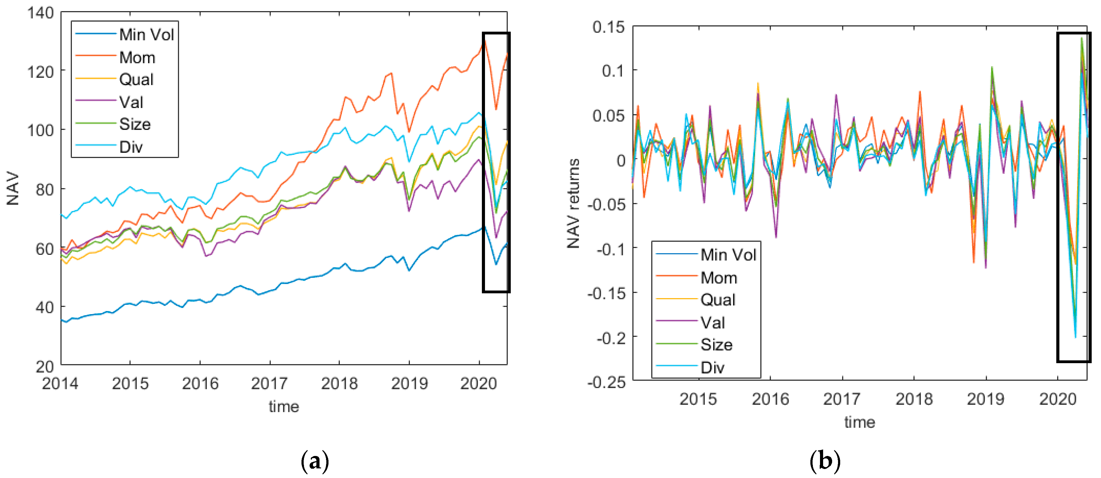
Figure 1 shows NAV values and time series of returns for all the smart beta considered, black rectangles highlight the COVID-19 period (January 2020–May 2020). From Figure 1a, note that NAV values start to sizably decrease in December 2019, and curves in Figure 1b show that the returns are characterized by a strong drop and then by a recovery during the COVID period. In order to investigate the existence of a correlation between multi-factor portfolio strategies and economic trends, the monthly macroeconomic time series are:
- Consumer price index for all urban consumers (CPI). This measures the average change in prices paid by consumers for a basket of consumer goods and services. It represents the main measure of inflation and is used as a basis for formulating monetary policy interventions and measuring the effectiveness of these measures.
- Real gross domestic product (GDP). This is the typical indicator of the volume of economic activity. It influences the decisions of all economic agents, from policy makers to individuals.
- Effective federal funds rate (FED rate for short). This represents the interest rate at which overnight transactions on federal deposits between financial institutions take place. This rate is a key lever for central banks when implementing decisions about monetary policy.
- CFE (CBOE Futures Exchange)–VIX Index (VIX). This financial index aims to provide a real-time estimate of the expected volatility on the S&P (Standard and Poor) 500 index in the following 30 days and consequently reflects the expectations of investors about the US stock market as a whole.
4. Discussion and Results
This section provides some evidence that portfolio dynamics, namely weight dynamics, are a good tool to reveal the link between smart beta strategies (“smart betas” for short) and macroeconomic variables. Specifically, in Section 4.1 we investigate the asset allocation strategies most suitable for evidencing this link while in Section 4.2 we show how the performance of these portfolios is closely connected to macroeconomics. Finally, in Section 4.3, we apply linear discriminant analysis for a robustness check in the choice of specific gain and loss thresholds as driver rules for the re-hedging activity.
4.1. Correlation Analysis
We start by motivating our choice of the macroeconomic variables GDP, CPI, and FED and the fear index VIX. To show that these four variables are able to capture the dynamics of the smart beta values, we use the following dynamic regression model:
Here, the error process,, in model (9) is described by the ARIMA(p, d, q) model in Equation (10), is a white noise series, and B is the backward shift operator (i.e., B = ). Specifically, p is the order of the autoregressive part, d is the order of the first differencing involved, and q is the order of the moving average part.
We apply model (9) and (10) to analyze the smart beta prices, , i = 1, 2, …, N, where N is the number of different smart betas considered. For any smart beta, the dependent variable, , is chosen in two different ways:
(a) the ratio between two consecutive prices of a smart beta (smart beta price ratio for short):
(b) the smart beta log-return:
We determine the best ARIMA process using the R function auto.arima() (see, Time Series Analysis with Auto.Arima in R|by Luis Losada|Towards Data Science for further details on the package).
Model (9) and (10) manages all spurious effects in the time series such as the presence of autocorrelation in the residuals. We consider the logarithm of the GDP to scale the value.
We have applied model (9) and (10) to the smart beta prices as a dependent variable and also investigated the dynamic regression of the smart beta price ratio as a dependent variable and macroeconomic variable. However, the results of these models provide weaker evidence of the link between smart beta and macroeconomics variables than the evidence of model (9) and (10) with dependent variables (a) and (b).
Table 3 shows the log-likelihood value (ML), AIC (Akaike) value, the standard error of the white noise (SE), and the coefficients associated with models (9) and (10).
The results displayed in Table 3 show that the explanatory variables are closely related to the prices and log-prices of the smart betas. Table A1 in Appendix A shows the results related to the autocorrelation in the residuals according to the Ljung-Box test. The estimated model violates the assumption of no autocorrelation in the errors in the cases of Min. Vol. price ratio and log returns as dependent variables for the period January 2014–May 2014 (Panel A); the coefficients are significant due to the unit-root problem, while some information is missed in the model. In the same Appendix A, Table A3 and Table A4 show the results of a lagged model to display the robustness of the results.
In general, COVID-19 leaves the relationship between smart beta and GDP or VIX more or less unchanged, but it reinforces the connection between the smart betas price ratio and the inflation/FED rate (see Table 3 Panel B, top and middle panels). This situation can be explained by the fact that smart betas act as “defenders” with respect to market anomalies, allowing for extra returns during times of crisis.
To obtain further evidence of this finding, we investigate the linear relationship between smart beta returns and the macroeconomic variables and VIX using the Pearson correlation. The results are displayed in Table 4.
The results show that there is a statistically significant correlation between the returns of all smart beta products and the VIX index, while the macroeconomic variables do not show significant correlations with smart betas except for the correlation between the FED rate and Quality ETF.
All significant coefficients are negative, which means that when market volatility increases, i.e., VIX increases, smart beta returns tend to fall and vice versa. Negative correlations are realistic due to the financial leverage of VIX and the US S&P 500 index. In particular, the negative correlation in the VIX/Size ETF pair may be due to the fact that small capitalization stocks are less liquid by nature. In the presence of a liquidity shortage that exacerbates spikes in the VIX index4, investors are induced to sell for fear of not being able to sell if the returns continue to fall.
VIX is a purely financial index that highlights the behavior and expectations of financial operators. Therefore, a considerable linear dependence with this index suggests the existence of a strong link between factors and the financial market.
In contrast, there is no linear dependence with the series most representative of economic cycle trends. Periods of expansion or recession, characterized by positive or negative GDP growth, as well as expansive or restrictive monetary policy (decrease or increase of the FED rate) or periods of inflation or deflation (increase or decrease in CPI) do not directly impact the performance of smart betas.
This is interesting for asset allocation purposes since only the smart beta returns seem to lead to a portfolio closely related to the VIX index. Is this true? Indeed, we expect a connection between a portfolio of smart betas and macroeconomic variables when a suitable allocation strategy is implemented.
Our main finding is that this linkage is hidden in the portfolio weight dynamics when the asset allocation is managed through a suitable compromise of risk and return.
Therefore, in contrast to smart beta returns, investing the optimal weights of a self-financing portfolio only in smart beta products and managing them with a prudent strategy shows significant correlations with the macroeconomic variables considered.
This expectation is motivated by two facts. On the one hand, smart beta price ratios and log returns are closely related to the macroeconomic variables (see Table 3 Panel A/B, top and middle panels). On the other hand, the macroeconomic variables cannot be assimilated into speculative assets so prudent strategies should reveal the connection.
As illustrated in Section 2, the liquidation of the entire portfolio when the rehedging rule is satisfied is implemented to force the hidden link between portfolio strategy and macroeconomic variables to emerge. In fact, thanks to this liquidation, rehedging accounts for the dynamics of all smart betas, thus indirectly accounting for the economic dynamics captured by the factors underlying the smart betas.
Hence, we first determine a strategy to reduce the correlation between VIX and portfolio weights and, then we analyze the portfolio weight dynamics as a function of the risk-aversion coefficient α. To pursue the first goal, we utilize three parameters: the largest admissible loss, γ, the largest admissible gain, ν, and the tail size, ψ, of the risk measure R; the risk-aversion coefficient α is used for the second objective.
As mentioned in the previous section, the largest loss and gain are fixed at 1% and 5%, respectively. These choices are prudent but rather realistic when no transaction costs are applied (see Shelton 2017), while the parameter α is used to understand the relationship between macroeconomic variables and risk aversion after reducing/eliminating the correlation with VIX. Therefore, the tail size, ψ, is determined to minimize the correlation between portfolio weights and the VIX index. To this end, we select the highest level of risk aversion (i.e., α = 0) and we consider different risk scenarios, choosing ψ equal to 0.6, 0.7, 0.8, and 0.9. The results are reported in Table 5.
Table 5 (Panel A and B) shows that when ψ moves from 0.60 to 0.90 and α = 0, the optimal weights of the smart beta portfolio are correlated with the VIX series up to ψ = 0.7, while this correlation disappears for larger values of ψ; that is, we do not find values statistically different from zero expect for those highlighted in gray.
This suggests that allowing for a higher probability of extreme losses not rewarded by higher returns because α is set to zero leads to a connection between weights and financial series that is volatile by nature. By adding the COVID period, the weights of Min. Vol. are correlated with VIX for higher values of ψ, while the link between the weights of Size and VIX remains unchanged suggesting that investors look for an extra return tied to less volatile assets.
We fix ψ = 0.8 and pursue the second objective; that is, we analyze the market timing portfolio as a function of the risk-aversion parameter α.
Table 6 shows correlations between smart beta weights and VIX for ψ = 0.8 and different values of α, specifically,. This is done to determine the values of the risk-aversion parameter, α, that make the portfolio dynamics uncorrelated with the fear index. These portfolio dynamics are worth further investigation to show the connection with the macroeconomic variables.
These correlations show that in moving towards scenarios more focused on profit, i.e., α closer to 1, the optimal weights of smart beta Size and VIX become more correlated; for lower values of α, however, investors are prone to invest in less volatile assets, i.e., minimum volatility product.
With regard to Table A7(a) and Table A8(a) in the Appendix B, note that the minimum volatility index is significantly and positively correlated with all the variables for more risk-averse investors (α = 0.1), i.e., an increase in GDP, CPI, FED, or VIX favors exposure to minimum volatility products, which allows higher market volatility to be contained in a crisis period characterized by the COVID-19 pandemic. Considering correlations of strategy size also leads to the same conclusion. The months of the COVID pandemic justify the negative correlation between the weights of the momentum strategy and macroeconomic/financial variables reflecting the tendency of investors to overreact to bad news regardless the value of alpha.
When we consider a portfolio entirely invested in financial ETFs5, the analysis of correlations shows similar results. ETF returns are correlated only with the VIX series, as shown in Table 7.
According to the correlation of optimal weights, ETFs are correlated with VIX only for ψ = 0.7, 0.9 when α = 0 as reported in Table 8.
Nevertheless, for ψ = 0.8, the relationship between ETFs and VIX occurs for lower values of α if we consider the time period excluding the COVID-19 pandemic (Table 9, Panel A).
Comparing Panels A and B in Table 9, the COVID period causes a move toward global (IXG) rather than local (IYF) ETFs, increasing significant links between the weights of IXG and VIX.
In Appendix B, Table A7(b) and Table A8(b) show correlations between the optimal weights and macroeconomic/financial time series considering α = 0.1, 0.9. The results show that for higher values of α, ETFs tend to be positively tied to the VIX variable; to obtain more remunerative portfolios, ETFs consider financial indices. On the contrary, the strategy of market timing on smart beta considers fluctuations of the economy as a whole.
We conclude by showing that the portfolio of the smart beta portfolio reveals the close link between these ETFs and the macroeconomic variables. To do so, we assess the link between the portfolio of smart betas and macroeconomic variables using the dynamic regression:
Here, as in the previous model, the error process,, in model (11) is described by ARIMA (p, d, q) model (i.e., Equation (12)), is a white noise series, B is the backward shift operator (i.e., B = ). Specifically, p is the order of the autoregressive part, d is the order of the first differencing involved and q the order of the moving average part. The dependent variable, is the portfolio ratio . We determine the best ARIMA process using the R function auto.arima().
Specifically, we test model (11)–(12) on portfolios of smart betas and financial ETFs for α = 0.1, 0.9 and ψ = 0.8. Model (11)–(12) is estimated by selecting the best ARIMA model that guarantees the error to be white noise. In Appendix A Table A2, we show the optimal choie of ARIMA model and the results of the Ljung-Box test. Moving from Panel A to Panel B in Table 10, note that the portfolio of smart betas remains tied to the VIX index for any level of risk aversion considered, but reinforcing the link between all other macroeconomic variables considered in the analysis. In a crisis period, the smart beta strategy reduces the speculative aspect of the portfolio, increasing the relationship with macroeconomic variables especially for less risk-averse individuals, where GDP, CPI, and FED show significant coefficients (for α = 0.9 CPI is not significant).
Table A2 in the Appendix A shows that in the case of financial ETF portfolios, the model violates the assumption of no autocorrelation in the residuals for α = 0.1, meaning that information is missed in the estimated model. The macroeconomic variables considered are not sufficient to explain the portfolio dynamics.
4.2. Portfolio Analysis
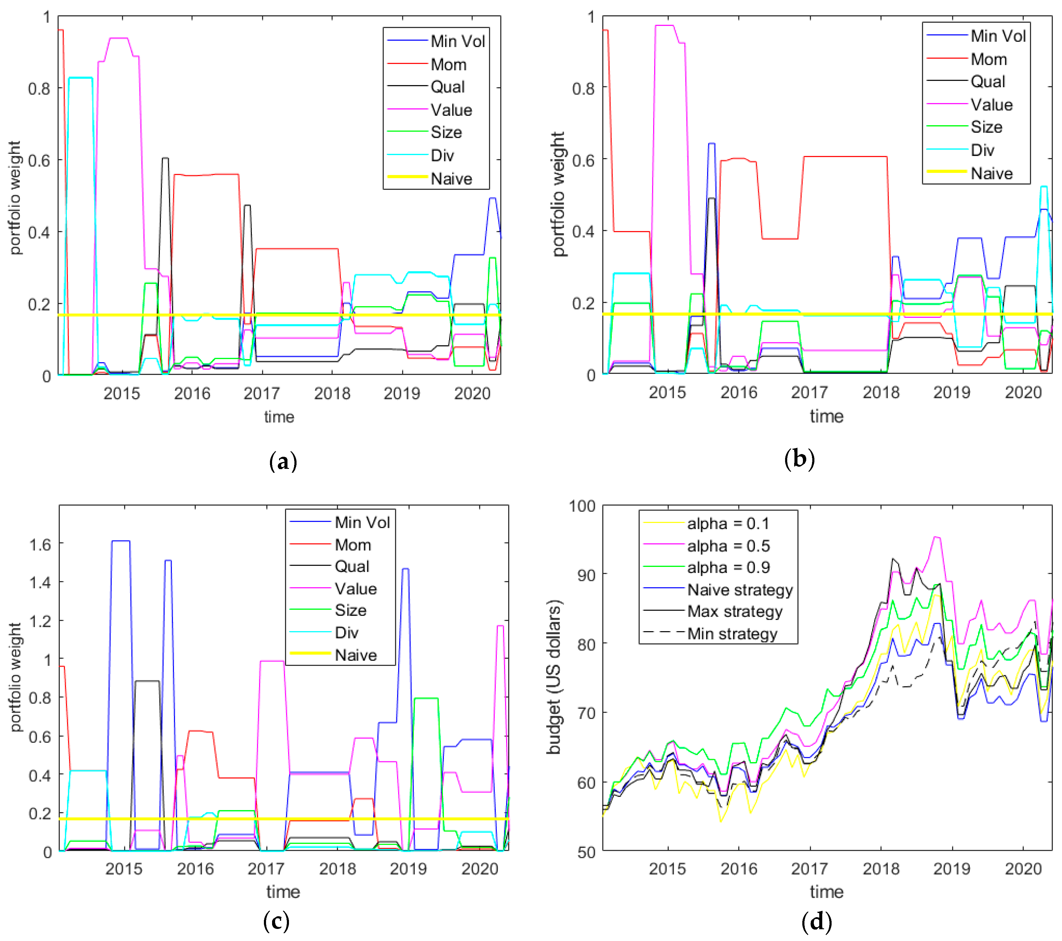
The coefficient α allows investors to choose a risk profile weighting suited to the two objectives of return and risk. We consider different values of α in order to show how the weights of smart beta products computed by solving Equation (2) vary over time with respect to the naive portfolio. Figure 3 shows the evolution of optimal weights for values of α equal to 0.1, 0.5, and 0.9, respectively in panels (a), (b), and (c), while the performances of all smart beta portfolios are compared in panel (d).
Bearing in mind that α is the risk propensity coefficient, the graphs show that, as expected, the portfolios are more diversified for low values of α: low risk aversion requires less concentrated portfolios.
When α = 0.9, dividend is not included in the portfolio for most of the time considered; the asset with the highest weight in the portfolio also changes over time at regular intervals.
From Figure 3a,b, it is interesting to note that, the weight of the minimum volatility strategy starts to increase at the end of 2019, meaning that the American market reacts to the COVID-19 news from China by investing in less volatile products. In contrast, more risk-prone investors represented by α = 0.9 do not invest in this strategy, a fact reflected in an underperforming portfolio during the year 2020 (Figure 3d, green line).
4.3. Forecasting via a Linear Discriminant Analysis
As mentioned in the previous sections, our proposed practical strategy permits to re-hedge portfolios only when it is possible to capitalize monthly gains (G) or losses (L), otherwise the portfolio is not updated (N). Thus, these three different occurrences are interpreted as a qualitative variable, named “tilting” variable, whose categories, G, L, N, depend on the smart beta dynamics.
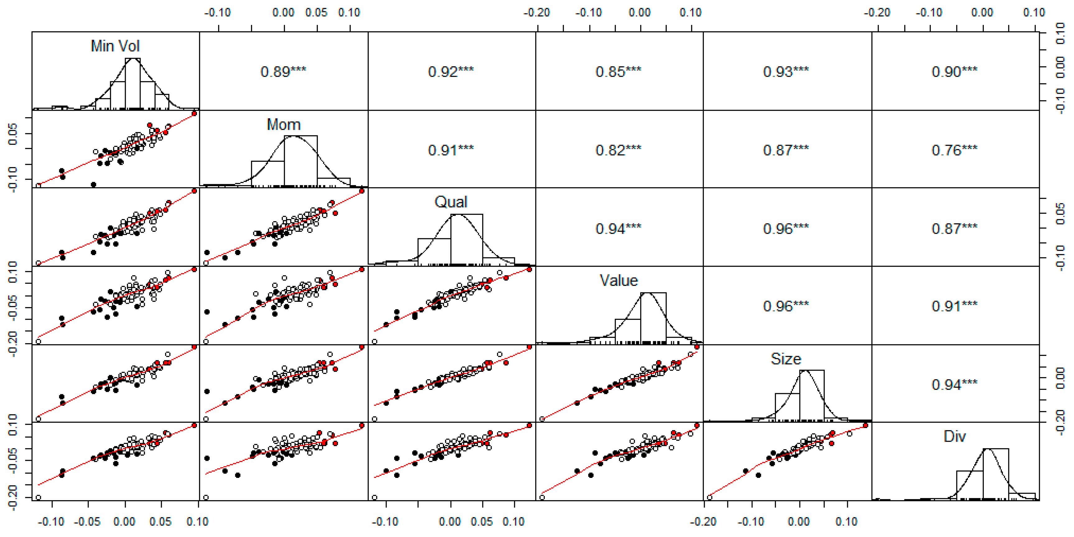
We investigate whether these three modes of the tilting variable can be distinguished through the observed smart beta returns. As shown in Figure 4, we start analyzing the bivariate scatter plot to determine pairs of smart beta showing high performance in discriminating losses and gains. From Figure 4, note that some smart betas better discriminate between gains and losses, or respectively from red to black circles, such as dividend and minimum volatility products regardless of other factor strategies coupled.
Since the tilting variable strongly depends on the threshold values, linear discriminant analysis (LDA) enables interesting results regarding these values in order to update portfolio weights and portfolio forecasting strategy.
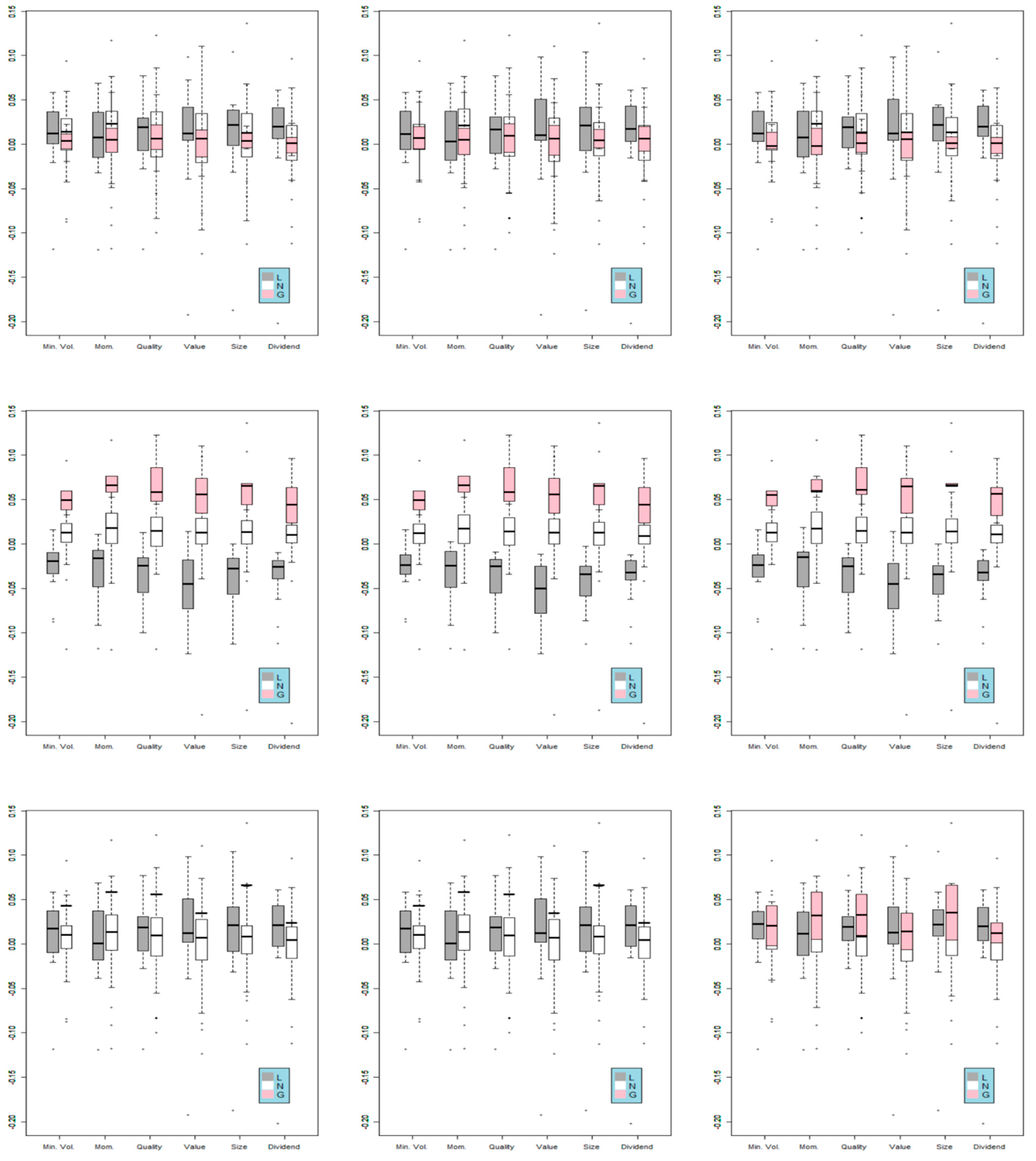
Moreover, Figure 5 shows an analysis of the returns according to tilting variable for different values of gain threshold, γ (2.5%, 5%, and 7.5%) and a fixed loss threshold, ν, of 1% to update portfolio weights.
The situation does not change if we consider different values of α (from left to right: 0.1, 0.5, 0.9) within each gain threshold. Differences can be seen between thresholds; indeed, when we consider a gain threshold value of 5% (middle panel), the average of smart beta products fluctuates around the loss and gain threshold values, 1% and 5%, respectively, or around 0 when the better strategy is represented by not rehedging.
Gain thresholds of 2.5% and 7% are not discriminant for the tilting variable: most of the time gains and losses are not distinguishable.
In addition, for each threshold, smart betas with small variances are more discriminant with respect to the tilting variable. For example, in the case of a gain threshold of 5%, Min. Vol., Mom, and Size products play an important role in gain capitalization, while Div products are important in the case of loss capitalization.
Table 11 confirms the fact that values set to 1% and 5% are reasonable and good discriminant thresholds to get portfolio dynamics “predictable and well-performing” for the values of α considered. This table shows scores associated with the first dimension of LDA according to different values of gain threshold.
Note that higher values of the first LDA coefficient are associated with the gain threshold of 5% regardless the value of α considered. This finding suggests that a gain threshold of 5% is the best choice to update portfolio weights according to Equation (2) and consequently, to detect a link between macroeconomic variables and smart betas.
The accuracy of the LDA described in Table 12 shows that the results are robust when lagged returns are considered in the analysis.
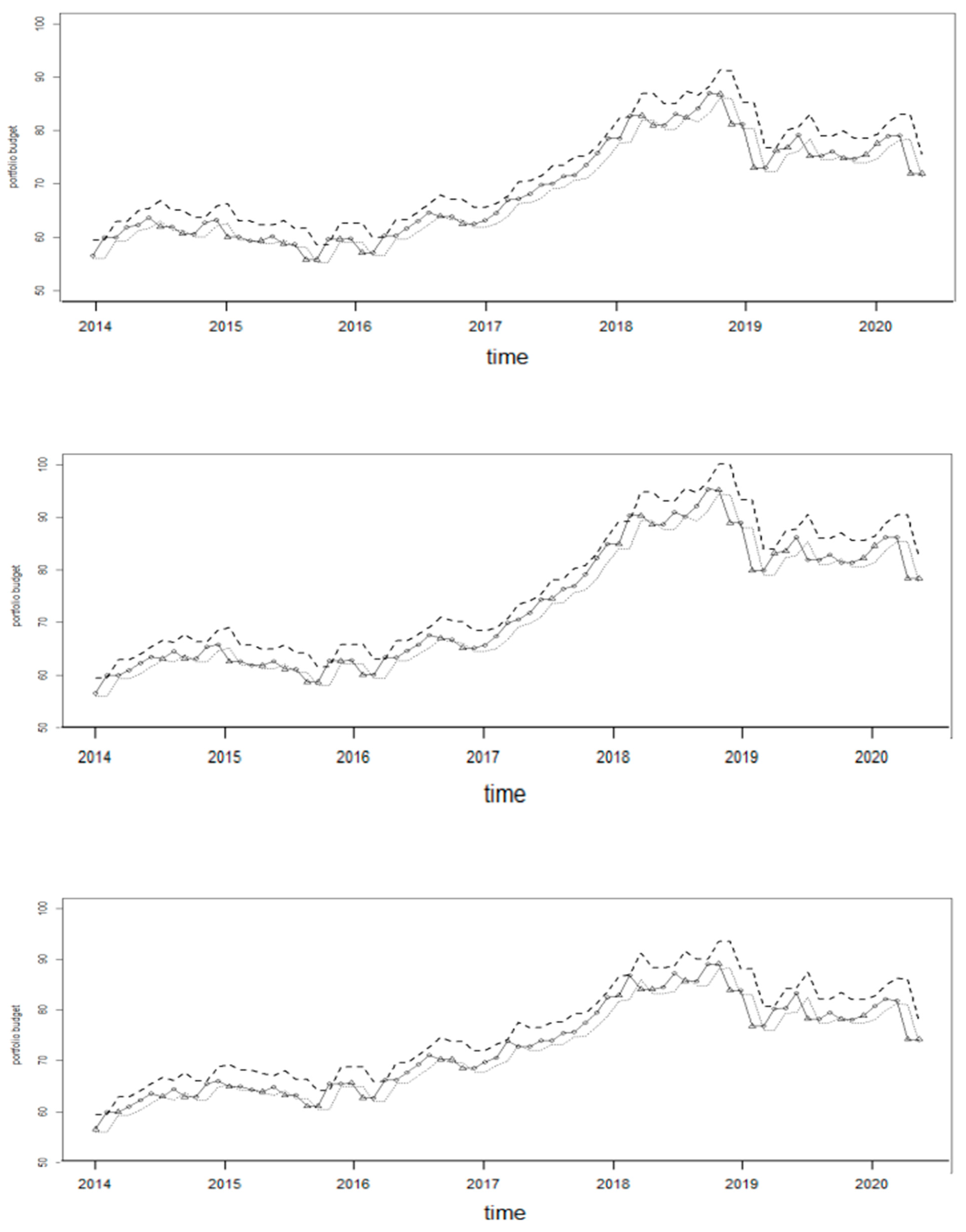
Moreover, we merge the two categories (gain and loss) of the tilting variable into the “rehedging” category in contrast to the “not rehedging” category to show results regarding the portfolio forecasting (see Figure 6)7.
The forecasting of portfolio rehedging is correct when triangles are out of the interval defined by lower and upper bounds, while the forecasting of the “not rehedging” is correct when the circle falls in the interval. Right prediction, i.e., triangles match budget out of bounds and circles budget within the bounds, occurs most of the time. Specifically, the accuracy of predictions is 79%, 72%, and 79% respectively for α = 0.1, 0.5 and 0.9.
The results of the LDA prediction based on the lagged smart beta returns allow us to detect the appropriate strategy represented by updating or not updating the portfolio weights one month in advance.
This fact emerges from Figure 6, which shows that the prediction of the appropriate strategy of rehedging at time t effectively occurs when the true value of the portfolio budget is above or below the threshold bounds most of the time.
5. Conclusions
Factor investing as the driving element of portfolio returns is well recognized in the literature. In particular, blended portfolios of smart beta strategies across economic regimes seek to address inefficiencies created by market-based indices, thereby enhancing investment returns above traditional benchmarks.
This paper assessed the effect of market timing activity on factor investing by detecting the relationship among optimal weights of smart betas and macroeconomic variables with a focus on the impact of the COVID-19 pandemic.
The empirical analysis shows a correlation between smart beta portfolio weights and the economy as a whole. Particularly, when the optimization process considers risk conditions, macroeconomic series influence portfolio weights while the financial series has no impact on the evolution of the portfolio itself. This finding is even more evident considering the COVID period.
Furthermore, market timing activity based on multi-factor portfolio strategies allows for the generation of portfolios that perform better than those entirely invested in financial ETFs or constructed by solving the Markowitz equation.
From a forecasting point of view, the technique used in the paper allows us to establish thresholds of gain and loss of 1% and 5%, respectively, which are reasonable and good discriminants for yielding portfolio dynamics that are “predictable and well-performing” for each level of risk aversion considered.
Future work will entail a study of the use of measures other than correlation coefficients to explain the relationship between smart beta products and macroeconomic variables.
Author Contributions
Conceptualization, M.F. and M.C.R.; methodology, M.C.R.; software, G.P.; supervision, M.C.R.; writing—original draft, G.P. and M.F. All authors have read and agreed to the published version of the manuscript.
Funding
This research received no external funding.
Institutional Review Board Statement
Not applicable.
Informed Consent Statement
Not applicable.
Data Availability Statement
Not applicable.
Conflicts of Interest
The authors declare no conflict of interest.
Appendix A

Table A1.
Details on the results of auto.arima() corresponding to model (9)–(10) in Table 3.
Table A1.
Details on the results of auto.arima() corresponding to model (9)–(10) in Table 3.
| Panel A—January 2014–May 2019 | |||
| Smart Beta Price Ratio | Arima (p,d,q) | p-Value | Model Degree of Freedom |
| Min. Vol. ETF | (1,0,0) | 0.0364 | 5 |
| Mom. ETF | (0,0,1) | 0.6049 | 5 |
| Qual. ETF | (0,0,1) | 0.1977 | 5 |
| Value ETF | (0,0,1) | 0.3296 | 6 |
| Size ETF | (0,0,1) | 0.3894 | 5 |
| Div. ETF | (1,0,0) | 0.5892 | 5 |
| Smart Beta Log-Return | Arima (p,d,q) | p-Value | Model Degree of Freedom |
| Min. Vol. ETF | (1,0,0) | 0.0410 | 5 |
| Mom. ETF | (0,0,1) | 0.6493 | 5 |
| Qual. ETF | (0,0,1) | 0.1871 | 5 |
| Value ETF | (0,0,1) | 0.2796 | 6 |
| Size ETF | (1,0,0) | 0.4782 | 5 |
| Div. ETF | (1,0,0) | 0.6235 | 5 |
| Panel B—January 2014–May 2020 | |||
| Smart Beta Price Ratio | Arima (p,d,q) | p-Value | Model Degree of Freedom |
| Min. Vol. ETF | (1,0,0) | 0.4017 | 6 |
| Mom. ETF | (2,0,0) | 0.3724 | 6 |
| Qual. ETF | (0,0,1) | 0.3802 | 5 |
| Value ETF | (1,0,1) | 0.3022 | 6 |
| Size ETF | (1,0,0) | 0.5546 | 5 |
| Div. ETF | (1,0,0) | 0.5726 | 5 |
| Smart Beta Return | Arima (p,d,q) | p-Value | Model Degree of Freedom |
| Min. Vol. ETF | (1,0,0) | 0.5089 | 5 |
| Mom. ETF | (2,0,0) | 0.3838 | 6 |
| Qual. ETF | (0,0,1) | 0.3846 | 5 |
| Value ETF | (1,0,1) | 0.2392 | 7 |
| Size ETF | (1,0,0) | 0.5426 | 5 |
| Div. ETF | (1,0,0) | 0.5016 | 5 |
Table A2.
Details on the results of auto.arima() corresponding to model (11)–(12) in Table 10.
Table A2.
Details on the results of auto.arima() corresponding to model (11)–(12) in Table 10.
| Panel A—January 2014–May 2019 | |||
| Model (11) for α = 0.1 | |||
| Portfolio | Arima (p,d,q) | p-Value | Model Degree of Freedom |
| Smart betas | (1,0,0) | 0.3616 | 5 |
| Financials | (0,0,0) | 0.1370 | 4 |
| Model (11) for α = 0.9 | |||
| Portfolio | Arima (p,d,q) | p-Value | Model Degree of Freedom |
| Smart betas | (1,0,0) | 0.1925 | 5 |
| Financials | (0,0,0) | 0.6422 | 4 |
| Panel B—January 2014–May 2020 | |||
| Model (11) for α = 0.1 | |||
| Portfolio | Arima (p,d,q) | p-Value | Model Degree of Freedom |
| Smart betas | (0,0,1) | 0.1889 | 5 |
| Financials | (0,0,0) | 0.0960 | 4 |
| Model (11) for α = 0.9 | |||
| Portfolio | Arima (p,d,q) | p-Value | Model Degree of Freedom |
| Smart betas | (2,0,0) | 0.1369 | 4 |
| Financials | (0,0,0) | 0.6675 | 5 |
To further check the robustness of the results, we consider the following model
applied to the price ratio (portfolio ratio). Table A3 is analogous to Table 3 while Table A4 is analogous to Table 10. We can see that Table A3 and Table A4 confirm the results of Table 3 and Table 10.
Table A3.
Results of model (A1)–(A2) on smart beta. Panel A includes data from January 2014 to May 2019, Panel B from January 2014 to May 20208.
Table A3.
Results of model (A1)–(A2) on smart beta. Panel A includes data from January 2014 to May 2019, Panel B from January 2014 to May 20208.
| Panel A | ||||||
| Model (A1)–(A2) for ETF price ratio | ||||||
| Smart Beta | ML | AIC (SE) | GDP | CPI | FED | VIX |
| Min. Vol. ETF | 148.43 | −284.86 (0.026) | 4.03 × 10⁻¹ (*) | −1.60 × 10⁻³ (-) | 7.30 × 10⁻³ (-) | −2.10 × 10⁻³ (*) |
| Mom. ETF | 130.57 | −249.14 (0.034) | 1.38 × 10⁻¹ (-) | 3.10 × 10⁻³ (-) | −2.56 × 10⁻² (-) | −3.00 × 10⁻³ (*) |
| Qual. ETF | 135.8 | −259.61 (0.031) | 1.52 × 10⁻¹ (-) | 2.80 × 10⁻³ (-) | −2.19 × 10⁻² (-) | −3.00 × 10⁻³ (**) |
| Value ETF | 137.01 | −258.02 (0.031) | 10.77 × 10⁻¹ (-) | 2.50 × 10⁻³ (-) | −2.21 × 10⁻² (-) | −4.00 × 10⁻³ (***) |
| Size ETF | 141.24 | −266.48 (0.029) | −5.20 × 10⁻³ (-) | −1.50 × 10⁻³ (-) | 1.24 × 10⁻² (-) | −2.40 × 10⁻³ (**) |
| Div. ETF | 147.95 | −283.9 (0.026) | 3.22 × 10⁻¹ (.) | −3.00 × 10⁻⁴ (-) | −4.70 × 10⁻³ (-) | −2.70 × 10⁻³ (**) |
| Panel B | ||||||
| Model (A1)–(A2) for ETF price ratio | ||||||
| Smart Beta | ML | AIC (SE) | GDP | CPI | FED | VIX |
| Min. Vol. ETF | 171.49 | −326.98 (0.027) | −4.44 × 10⁻¹ (-) | 7.0 × 10⁻⁴ (-) | 5.70 × 10⁻³ (-) | 2.50 × 10⁻³ (***) |
| Mom. ETF | 154.89 | −293.78 (0.034) | 1.57 × 10⁻¹ (**) | 1.30 × 10⁻³ (-) | −1.31 × 10⁻² (.) | −2.60 × 10⁻³ (***) |
| Qual. ETF | 159.13 | −304.27 (0.032) | 1.98 × 10⁻¹ (***) | 6.00 × 10⁻⁴ (-) | −7.30 × 10⁻³ (**) | −2.00 × 10⁻³ (**) |
| Value ETF | 156.32 | −298.65 (0.033) | 1.96 × 10⁻¹ (***) | 1.20 × 10⁻³ (***) | −1.46 × 10⁻² (***) | −4.00 × 10⁻³ (***) |
| Size ETF | 156.5 | −299.01 (0.033) | 2.36 × 10⁻¹ (***) | 7.00 × 10⁻⁴ (-) | −9.80 × 10⁻³ (-) | −3.70 × 10⁻³ (***) |
| Div. ETF | 163.03 | −312.06 (0.030) | 2.79 × 10⁻¹ (***) | −2.00 × 10⁻⁴ (-) | −3.90 × 10⁻³ (-) | −3.50 × 10⁻³ (***) |
Table A4.
Results of model (A1)–(A2) (Panels A and B) applied to smart beta and financial ETF portfolios. Panel A includes data from January 2014 to May 2019, Panel B from January 2014 to May 20209.
Table A4.
Results of model (A1)–(A2) (Panels A and B) applied to smart beta and financial ETF portfolios. Panel A includes data from January 2014 to May 2019, Panel B from January 2014 to May 20209.
| Panel A—January 2014–May 2019 | ||||||
| Model (A1)–(A2) for α = 0.1 | ||||||
| Portfolio | ML | AIC (Res. SE) | GDP | CPI | FED | VIX |
| Smart betas | 126.93 | −241.87 (0.036) | −4.56 × 10⁻² (-) | 6.70 × 10⁻³ (-) | −5.12 × 10⁻² (.) | −2.70 × 10⁻³ (*) |
| Financials | 37.17 | −62.34 (0.142) | 3.52 × 10⁻¹ (-) | −1.64 × 10⁻³ (-) | 1.60 × 10⁻² (-) | −6.03 × 10⁻³ (-) |
| Model (A1)–(A2) for α = 0.9 | ||||||
| Portfolio | ML | AIC (Res. SE) | GDP | CPI | FED | VIX |
| Smart betas | 120.05 | −228.1 (0.040) | 7.69 × 10⁻¹ (-) | 4.70 × 10⁻³ (-) | −4.01 × 10⁻² (-) | −2.40 × 10⁻³ (.) |
| Financials | −45.15 | 102.34 (0.504) | 8.82 × 10⁻¹ (*) | −1.54 × 10⁻¹ (*) | 1.13 × 10⁻¹ (*) | 2.03 × 10⁻² (-) |
| Panel B—January 2014–May 2020 | ||||||
| Model (A1)–(A2) for α = 0.1 | ||||||
| Portfolio | ML | AIC (SE) | GDP | CPI | FED | VIX |
| Smart betas | 145.46 | −274.92 (0.038) | 8.12 × 10⁻² (*) | 1.30 × 10⁻³ (***) | −1.32 × 10⁻² (***) | −1.60 × 10⁻³ (***) |
| Financials | 49.24 | −86.47 (0.132) | 1.18 × 10⁻¹ (-) | 2.62 × 10⁻³ (-) | −1.83 × 10⁻² (-) | −5.84 × 10⁻³ (*) |
| Model (A1)–(A2) for α = 0.9 | ||||||
| Portfolio | ML | AIC (SE) | GDP | CPI | FED | VIX |
| Smart betas | 136.24 | −256.47 (0.043) | 1.29 × 10⁻¹ (*) | 1.30 × 10⁻³ (-) | −1.52 × 10⁻² (.) | −1.70 × 10⁻³ (**) |
| Financials | −85.57 | 187.14 (0.770) | 34.98 × 10⁻¹ (.) | −6.44 × 10⁻² (.) | −1.41 × 10⁻¹ (-) | 1.62 × 10⁻¹ (***) |
Table A5.
Details on the results of auto.arima() corresponding to model (A1)–(A2) in Table A3.
Table A5.
Details on the results of auto.arima() corresponding to model (A1)–(A2) in Table A3.
| Panel A—January 2014–May 2019 | |||
| Smart Beta Price Ratio | Arima (p,d,q) | p-Value | Model Degree of Freedom |
| Min. Vol. ETF | (0,0,0) | 0.0309 | 5 |
| Mom. ETF | (0,0,0) | 0.4397 | 5 |
| Qual. ETF | (0,0,0) | 0.2523 | 5 |
| Value ETF | (2,0,0,) | 0.4196 | 7 |
| Size ETF | (0,0,1) | 0.1295 | 7 |
| Div. ETF | (0,0,0) | 0.5715 | 5 |
| Panel B—January 2014–May 2020 | |||
| Smart Beta Price Ratio | Arima (p,d,q) | p-Value | Model Degree of Freedom |
| Min. Vol. ETF | (1,0,0) | 0.2608 | 7 |
| Mom. ETF | (2,0,0) | 0.2378 | 7 |
| Qual. ETF | (0,0,1) | 0.3344 | 6 |
| Value ETF | (0,0,1) | 0.1484 | 6 |
| Size ETF | (1,0,0) | 0.4414 | 6 |
| Div. ETF | (1,0,0) | 0.3968 | 6 |
Table A6.
Details on the results of auto.arima() corresponding to model (A1)–(A2) in Table A4.
Table A6.
Details on the results of auto.arima() corresponding to model (A1)–(A2) in Table A4.
| Panel A—January 2014–May 2019 | |||
| Model (A1)–(A2) for α = 0.1 | |||
| Portfolio | Arima (p,d,q) | p-Value | Model Degree of Freedom |
| Smart betas | (0,0,0) | 0.2593 | 5 |
| Financials | (0,0,0) | 0.0804 | 5 |
| Model (A1)–(A2) for α = 0.9 | |||
| Portfolio | Arima (p,d,q) | p-Value | Model Degree of Freedom |
| Smart betas | (0,0,0) | 0.1647 | 5 |
| Financials | (0,0,0) | 0.5326 | 5 |
| Panel B—January 2014–May 2020 | |||
| Model (A1)–(A2) for α = 0.1 | |||
| Portfolio | Arima (p,d,q) | p-Value | Model Degree of Freedom |
| Smart betas | (1,0,1) | 0.1078 | 7 |
| Financials | (0,0,0) | 0.0493 | 5 |
| Model (A1)–(A2) for α = 0.9 | |||
| Portfolio | Arima (p,d,q) | p-Value | Model Degree of Freedom |
| Smart betas | (2,0,0) | 0.0856 | 7 |
| Financials | (0,0,1) | 0.1614 | 7 |
Appendix B
Table A7.
Correlation between optimal weights of smart beta (a) and ETFs (b) and macroeconomic variables for α = 0. Significant correlations (5% significant level) are highlighted by gray color.
Table A7.
Correlation between optimal weights of smart beta (a) and ETFs (b) and macroeconomic variables for α = 0. Significant correlations (5% significant level) are highlighted by gray color.
| (a) | (b) | ||||||||||||
|---|---|---|---|---|---|---|---|---|---|---|---|---|---|
| Min. Vol | Mom. | Qual. | Value | Size | Div. | DIA | IHI | IXG | IYF | IYG | SPY | ||
| GDP | 0.597 | −0.2329 | 0.1596 | −0.3022 | 0.4931 | −0.0262 | GDP | 0.0782 | −0.3311 | 0.5027 | 0.1839 | 0.4329 | −0.0912 |
| VIX | 0.5253 | −0.1325 | 0.0072 | −0.0432 | 0.2198 | −0.0412 | VIX | 0.0106 | 0.0955 | −0.1065 | −0.2016 | −0.3073 | −0.1219 |
| CPI | 0.8726 | −0.3416 | 0.1522 | −0.3433 | 0.521 | 0.0678 | CPI | −0.0612 | −0.2061 | 0.3833 | 0.0341 | 0.2382 | −0.0492 |
| FED | 0.557 | −0.2653 | 0.0459 | −0.3073 | 0.5318 | 0.121 | FED | −0.0267 | −0.1767 | 0.4603 | 0.1304 | 0.3213 | −0.0817 |
Table A8.
Correlation between optimal weights of smart beta (a) and ETFs (b) and macroeconomic variables for α = 0.9. Significant correlations (5% significant level) are highlighted by gray color.
Table A8.
Correlation between optimal weights of smart beta (a) and ETFs (b) and macroeconomic variables for α = 0.9. Significant correlations (5% significant level) are highlighted by gray color.
| (a) | (b) | ||||||||||||
|---|---|---|---|---|---|---|---|---|---|---|---|---|---|
| Min.Vol | Mom. | Qual. | Value | Size | Div. | DIA | IHI | IXG | IYF | IYG | SPY | ||
| GDP | 0.1475 | −0.5254 | −0.2013 | 0.2965 | 0.317 | −0.432 | GDP | 0.2851 | −0.3889 | −0.0453 | −0.0493 | 0.0127 | −0.1147 |
| VIX | 0.0092 | −0.0707 | −0.0893 | 0.2619 | −0.0239 | −0.1293 | VIX | −0.0706 | −0.1148 | 0.3874 | −0.0259 | −0.1987 | −0.1485 |
| CPI | 0.1146 | −0.5371 | −0.2803 | 0.4127 | 0.2864 | −0.3635 | CPI | 0.2608 | −0.2706 | −0.0303 | −0.0924 | −0.0503 | −0.2126 |
| FED | 0.1463 | −0.4599 | −0.2523 | 0.2099 | 0.4195 | −0.3926 | FED | 0.3131 | −0.2782 | −0.0417 | −0.0827 | −0.0761 | −0.1443 |
References
- Amenc, Noel, Felix Goltz, Ashish Lodh, and Lionel Martellini. 2012. Diversifying the Diversifiers and Tracking the Tracking Error: Outperforming Cap-Weighted Indices with Limited Risk of Underperformance. The Journal of Portfolio Management 38: 72–88. [Google Scholar] [CrossRef] [Green Version]
- Amenc, Noel, Felix Goltz, Ashish Lodh, and Lionel Martellini. 2014. Towards Smart Equity Factor Indices: Harvesting Risk Premia Without Taking Unrewarded Risks. The Journal of Portfolio Management 40: 106–22. [Google Scholar] [CrossRef] [Green Version]
- Ang, Andrew. 2014. Asset Management: A Systematic Approach to Factor Investing. Oxford: Oxford University Press. [Google Scholar]
- Arnott, Robert D., Jason Hsu, and Philip Moore. 2005. Fundamental Indexation. Financial Analysts Journal 61: 83–99. [Google Scholar] [CrossRef]
- Asness, Clifford, Andrea Frazzini, Ronen Israel, Tobias J. Moskowitz, and Lasse H. Pedersen. 2018. Size Matters, If You Control Your Junk. Journal of Financial Economics 129: 479–509. [Google Scholar] [CrossRef]
- Autier, Benoit, Mike McGlone, and Alexander Channig. 2016. Smart Beta 2.0. Bringing Clarity to Equity Smart Beta. Sydney: ETF Securities. [Google Scholar]
- Banz, Rolf. W. 1981. The Relationship Between Return and Market Value of Common Stocks. Journal of Financial Economics 9: 3–18. [Google Scholar] [CrossRef] [Green Version]
- Basu, Sanjoy. 1977. Investment Performance of Common Stocks in Relation to Their Price-Earnings Ratios: A Test of the Efficient Market Hypothesis. The Journal of Finance 32: 663–82. [Google Scholar] [CrossRef]
- Bender, Jennifer, Remy Briand, Dimitris Melas, Raman A. Subramanian, and Madhu Subramanian. 2013. Deploying Multi-Factor Index Allocations in Institutional Portfolios. New York: MSCI Research Insights. [Google Scholar]
- Brière, Marie, and Ariane Szafarz. 2020. Good Diversification Is Never Wasted: How to Tilt Factor Portfolios with Sectors. Finance Research Letters 33: 101197. [Google Scholar] [CrossRef] [Green Version]
- Carhart, Mark M. 1997. On Persistence in Mutual Fund Performance. The Journal of Finance 52: 57–82. [Google Scholar] [CrossRef]
- Dichtl, Hubert, Wolfgang Drobetz, Harald Lohre, Carsten Rother, and Patrick Vosskamp. 2019. Optimal timing and tilting of equity factors. Financial Analysts Journal 75: 84–102. [Google Scholar] [CrossRef]
- Fama, Eugene F., and Kenneth R. French. 1992. The Cross-Section of Expected Stock Returns. The Journal of Finance 47: 427–65. [Google Scholar] [CrossRef]
- Fama, Eugene F., and Kenneth R. French. 2006. Profitability, Investment and Average Returns. Journal of Financial Economics 82: 491–518. [Google Scholar] [CrossRef]
- Fama, Eugene F., and Kenneth R. French. 2012. Size, Value, and Momentum in International Stock Returns. Journal of Financial Economics 105: 457–72. [Google Scholar] [CrossRef]
- Fama, Eugene F., and Kenneth R. French. 2015. A Five-Factor Asset Pricing Model. Journal of Financial Economics 116: 1–22. [Google Scholar] [CrossRef] [Green Version]
- FTSE Russell Smart Beta Survey. 2016. Smart Beta: 2016 Global Survey Findings from Asset Owners. London: FTSE Russell. [Google Scholar]
- Ghayur, Khalid, Ronan Heaney, and Stephen Platt. 2018. Constructing Long-Only Multifactor Strategies: Portfolio Blending Vs. Signal Blending. Financial Analysts Journal 74: 70–85. [Google Scholar] [CrossRef]
- Hou, Kewei, Chen Xue, and Lu Zhang. 2015. Digesting Anomalies: An Investment Approach. The Review of Financial Studies 28: 650–705. [Google Scholar] [CrossRef] [Green Version]
- Hunjra, Ahmed I., Suha Alawi, Sisira Colombage, Uroosa Sahito, and Mahnoor Hanif. 2020. Portfolio Construction by Using Different Risk Models: A Comparison among Diverse Economic Scenarios. Risks 8: 126. [Google Scholar] [CrossRef]
- Malkiel, Burton G., and Eugene F. Fama. 1970. Efficient Capital Markets: A Review of Theory and Empirical Work. The Journal of Finance 25: 383–417. [Google Scholar] [CrossRef]
- Markovich, Michael, and Rasmus Rousing. 2016. Equity Style Investing—Guidelines for Style Rotation. Zurich: Credit Suisse, International Wealth Management. [Google Scholar]
- Markowitz, Harry. 1952. Portfolio Selection. The Journal of Finance 7: 77–91. [Google Scholar]
- Marsh, Terry, and Paul Pfleiderer. 2016. Alpha Signals Smart Betas and Factor Model Alignment. The Journal of Portfolio Management 42: 51–66. [Google Scholar] [CrossRef]
- Martellini, Lionel. 2010. Alternatives to Cap-Weighted Indices. Investment & Pensions Europe 83: 2. [Google Scholar]
- Novy-Marx, Robert. 2013. The Other Side of Value: The Gross Profitability Premium. Journal of Financial Economics 108: 1–28. [Google Scholar] [CrossRef] [Green Version]
- Rigamonti, Andrea. 2020. Mean-variance optimization is a good choice, but for other reasons than you might think. Risks 8: 29. [Google Scholar] [CrossRef] [Green Version]
- Sharpe, William F. 1964. Capital Asset Prices: A Theory of Market Equilibrium Under Conditions of Risk. The Journal of Finance 19: 425–42. [Google Scholar]
- Shelton, Austin. 2017. The Value of Stop-Loss, Stop-Gain Strategies in Dynamic Asset Allocation. Journal of Asset Management 18: 124–43. [Google Scholar] [CrossRef]
- Xing, Yuhang. 2008. Interpreting the Value Effect Through the Q-Theory: An Empirical Investigation. The Review of Financial Studies 21: 1767–95. [Google Scholar] [CrossRef] [Green Version]
| 1 | Transaction costs of 1% are considered only when the monthly rehedging occurs. |
| 2 | Tables in the paper consider the period January 2014–May 2020; two periods are considered when there are differences to be highlighted and they are respectively January 2014–May 2019 and January 2014–May 2020. Tables referring to the first period are shown in the supplementary material of the paper. |
| 3 | Significance codes: p-value ≤ 0.001 (***); (**) 0.001 < p-value ≤ 0.01; (*) 0.01 < p-value ≤ 0.05; (·) 0.05 < p-value ≤ 0.1; (-) 0.1 < p-value ≤ 1. |
| 4 | |
| 5 | The ticker symbols of financial ETFs considered in the analysis are DIA, IXG, IHI, IYF, IYG, and SPY. |
| 6 | Significance codes: p-value ≤ 0.001 (***); (**) 0.001 < p-value ≤ 0.01; (*) 0.01 < p-value ≤ 0.05; (·) 0.05 < p-value ≤ 0.1; (-) 0.1 < p-value ≤ 1. |
| 7 | In Figure 6, the symbols represent the observed tilting variable (rehedging-triangle or not rehedging-circle) according to the LDA prediction at time t − 2, which provides the forecast of the tilting variable at t −1. The accuracy of this prediction is assessed at time t. |
| 8 | Significance codes: p-value ≤ 0.001 (***); (**) 0.001 < p-value ≤ 0.01; (*) 0.01 < p-value ≤ 0.05; (·) 0.05 < p-value ≤ 0.1;(-) 0.1 < p-value ≤ 1. |
| 9 | Signif. codes: p-value ≤ 0.001 (***); (**) 0.001 < p-value ≤ 0.01; (*) 0.01 < p-value ≤ 0.05; (·) 0.05 < p-value ≤ 0.1; (-) 0.1 < p-value ≤ 1. |
Figure 1.
Monthly net asset value (NAV) in US dollars (a) and log returns (b) of smart beta products from January 2014 to May 2020. Source: Datastream.
Figure 1.
Monthly net asset value (NAV) in US dollars (a) and log returns (b) of smart beta products from January 2014 to May 2020. Source: Datastream.

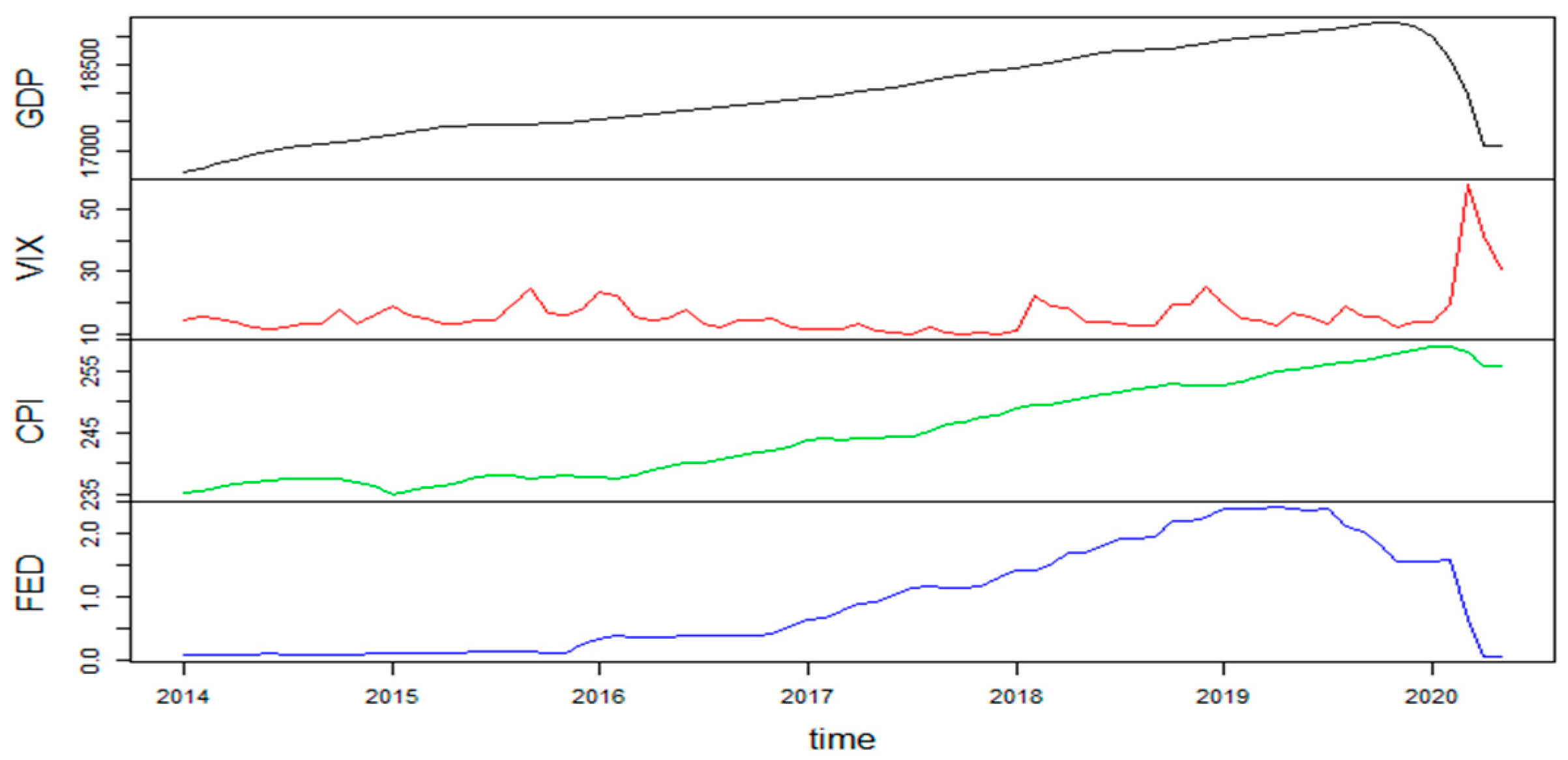
Figure 2.
Monthly data as a function of the time period January 2014–May 2020: FED (effective federal funds rate) and VIX (volatility index) (percent) gross domestic product (GDP) and consumer price index (CPI) (US dollars). Source: Datastream.
Figure 2.
Monthly data as a function of the time period January 2014–May 2020: FED (effective federal funds rate) and VIX (volatility index) (percent) gross domestic product (GDP) and consumer price index (CPI) (US dollars). Source: Datastream.

Figure 3.
Portfolio optimal weights for α equal to 0.1 (a), 0.5 (b), 0.9 (c), and portfolio performances (budget expressed in US dollars) for all strategies considered (d) from January 2014 to May 2020. Source: our elaboration on data.
Figure 3.
Portfolio optimal weights for α equal to 0.1 (a), 0.5 (b), 0.9 (c), and portfolio performances (budget expressed in US dollars) for all strategies considered (d) from January 2014 to May 2020. Source: our elaboration on data.

Figure 4.
Bivariate scatter plots below the diagonal, histograms on the diagonal, and the Pearson correlation above the diagonal. Points represent the grouping variables G (red), L (black), and N (white). Source: our elaboration on data. Period: January 2014–May 2020. p-value ≤ 0.001 (***).
Figure 4.
Bivariate scatter plots below the diagonal, histograms on the diagonal, and the Pearson correlation above the diagonal. Points represent the grouping variables G (red), L (black), and N (white). Source: our elaboration on data. Period: January 2014–May 2020. p-value ≤ 0.001 (***).

Figure 5.
Box plots of smart beta returns for different tilting investment variables (G, L, N), gain threshold values (from top to bottom: 2.5%, 5%, and 7.5%), and values of alpha (from left to right: 0.1, 0.5, 0.9). Source: our elaboration on data. (**) 0.001 < p-value ≤ 0.01; (*) 0.01 < p-value ≤ 0.05.

Figure 6.
The solid line shows the true value of the portfolio budget while upper and lower bounds are computed as 5% and 1% of the portfolio budget at time t. Upper panel α = 0.1, middle panel α = 0.5, and bottom panel α = 0.9. Source: our computation on data. Period: January 2014–May 2020.
Figure 6.
The solid line shows the true value of the portfolio budget while upper and lower bounds are computed as 5% and 1% of the portfolio budget at time t. Upper panel α = 0.1, middle panel α = 0.5, and bottom panel α = 0.9. Source: our computation on data. Period: January 2014–May 2020.

Table 1.
Exchange traded funds (ETF) return summary statistics. Summary statistics for exchange traded funds: mean, standard deviation, excess of kurtosis, and skewness. Panel A includes data from January 2014 to May 2019, Panel B from January 2014 to May 2020.
Table 1.
Exchange traded funds (ETF) return summary statistics. Summary statistics for exchange traded funds: mean, standard deviation, excess of kurtosis, and skewness. Panel A includes data from January 2014 to May 2019, Panel B from January 2014 to May 2020.
| Panel A | |||||
| ETF Name | Benchmark | Mean | SD | Kurt. | Skew. |
| 1 ISHARES EDGE MSCI MIN VOL USA | MSCI USA Minimum Volatility Index | 0.008 | 0.027 | 0.83 | −0.54 |
| 2 ISHARES EDGE MSCI USA MOMENTUM FACTOR | MSCI USA Momentum Index | 0.01 | 0.036 | 1.62 | −0.87 |
| 3 ISHARES EDGE MSCI USA QUALITY FACTOR | MSCI USA Sector Neutral Quality Index | 0.007 | 0.034 | 0.94 | −0.51 |
| 4 ISHARES EDGE MSCI USA VALUE FACTOR | MSCI USA Enhanced Value Index | 0.005 | 0.039 | 1.29 | −0.62 |
| 5 ISHARES EDGE MSCI USA SIZE FACTOR | MSCI USA Risk Weighted Index | 0.007 | 0.034 | 1.83 | −0.50 |
| 6 ISHARES SELECT DIVIDEND | Dow Jones U.S. Selected Dividend Index | 0.005 | 0.029 | 1.09 | −0.57 |
| Panel B | |||||
| ETF Name | Benchmark | Mean | SD | Kurt. | Skew. |
| 1 ISHARES EDGE MSCI MIN VOL USA | MSCI USA Minimum Volatility Index | 0.001 | 0.033 | 2.90 | −1.02 |
| 2 ISHARES EDGE MSCI USA MOMENTUM FACTOR | MSCI USA Momentum Index | 0.01 | 0.040 | 1.77 | −0.79 |
| 3 ISHARES EDGE MSCI USA QUALITY FACTOR | MSCI USA Sector Neutral Quality Index | 0.008 | 0.040 | 1.54 | −0.51 |
| 4 ISHARES EDGE MSCI USA VALUE FACTOR | MSCI USA Enhanced Value Index | 0.004 | 0.047 | 3.25 | −1.15 |
| 5 ISHARES EDGE MSCI USA SIZE FACTOR | MSCI USA Risk Weighted Index | 0.006 | 0.044 | 4.74 | −1.03 |
| 6 ISHARES SELECT DIVIDEND | Dow Jones U.S. Selected Dividend Index | 0.003 | 0.040 | 7.99 | −1.94 |
Table 2.
Summary statistics of macroeconomic and financial time series from January 2014 to May 2020: FED and VIX (percent) GDP and CPI (US dollars). Source: Datastream.
Table 2.
Summary statistics of macroeconomic and financial time series from January 2014 to May 2020: FED and VIX (percent) GDP and CPI (US dollars). Source: Datastream.
| Mean | SD | Kurt. (Excess) | Skew. | |
|---|---|---|---|---|
| GDP | 17,876.56 | 829.53 | −1.19 | 0.07 |
| FED | 0.92 | 0.83 | −1.27 | 0.52 |
| CPI | 245.12 | 7.80 | −1.42 | 0.32 |
| VIX | 16.15 | 6.83 | 17.72 | 3.71 |
Table 3.
Results of model (9) and (10) on smart beta. Panel A includes data from January 2014 to May 2019, Panel B from January 2014 to May 20203.
Table 3.
Results of model (9) and (10) on smart beta. Panel A includes data from January 2014 to May 2019, Panel B from January 2014 to May 20203.
| Panel A | ||||||
| Model (9)–(10) for ETF Price Ratio | ||||||
| Smart Beta | ML | AIC (SE) | GDP | CPI | FED | VIX |
| Min. Vol. ETF | 150.1 | −288.32 (0.025) | 3.95 × 10⁻¹ (**) | −2.67 × 10⁻³ (-) | 1.52 × 10⁻² (-) | −2.34 × 10⁻³ (**) |
| Mom. ETF | 135.1 | −285.13 (0.034) | 3.28 × 10⁻¹ (*) | −1.38 × 10⁻³ (-) | 5.26 × 10⁻¹³ (-) | −3.53 × 10⁻³ (***) |
| Qual. ETF | 153.6 | −295.24 (0.034) | 2.77 × 10⁻¹ (*) | −5.34 × 10⁻⁴ (-) | 4.75 × 10⁻⁴ (-) | −2.91 × 10⁻³ (***) |
| Value ETF | 137.5 | −263.08 (0.030) | −1.30 × 10⁻¹ (-) | 3.17 × 10⁻³ (-) | −2.34 × 10⁻² (*) | −3.29 × 10⁻³ (***) |
| Size ETF | 140.8 | −269.55 (0.028) | 3.71 × 10⁻¹ (**) | −2.20 × 10⁻³ (-) | 1.11 × 10⁻² (-) | −2.93 × 10⁻³ (***) |
| Div. ETF | 148.7 | −285.42 (0.026) | 3.19 × 10⁻¹ (*) | −1.30 × 10⁻³ (-) | −3.66 × 10⁻³ (-) | −262 × 10−3 (**) |
| Model (9)–(10) for ETF log-returns | ||||||
| Smart Beta | ML | AIC (SE) | GDP | CPI | FED | VIX |
| Min. Vol. ETF | 150.51 | −289.03 (0.025) | 1.27 × 10⁻¹ (-) | −2.10 × 10⁻³ (-) | 1.56 × 10⁻² (-) | −2.35 × 10⁻³ (**) |
| Mom. ETF | 134.27 | −256.53 (0.032) | 4.49 × 10⁻² (-) | −5.37 × 10⁻³ (-) | 3.63 × 10⁻³ (-) | 3.60 × 10⁻³ (***) |
| Qual. ETF | 138.46 | −264.91 (0.03) | 3.40 × 10⁻³ (-) | 1.51 × 10⁻⁴ (-) | −8.73 × 10⁻⁵ (-) | −2.92 × 10⁻³ (***) |
| Value ETF | 138.23 | −262.45 (0.03) | −1.73 × 10⁻¹ (-) | 3.49 × 10⁻³ (.) | −2.55 × 10⁻² (*) | −3.30 × 10⁻³ (***) |
| Size ETF | 141.13 | −270.26 (0.03) | 8.15 × 10⁻² (-) | −1.21 × 10⁻³ (-) | 8.96 × 10⁻³ (-) | −3.60 × 10⁻³ (***) |
| Div. ETF | 148.84 | −285.68 (0.025) | 5.056 × 10⁻² (-) | −7.16 × 10⁻⁴ (-) | 4.03 × 10⁻³ (-) | −3.00 × 10⁻³ (***) |
| Panel B | ||||||
| Model (9)–(10) for ETF Price Ratio | ||||||
| Smart Beta | ML | AIC (SE) | GDP | CPI | FED | VIX |
| Min. Vol. ETF | 171.5 | −328.91 (0.027) | −4.66 × 10⁻¹ (-) | 7.24 × 10⁻⁴ (-) | 5.59 × 10⁻³ (-) | −2.48 × 10⁻³ (***) |
| Mom. ETF | 154.7 | −295.49 (0.033) | 1.74 × 10⁻¹ (***) | 1.32 × 10⁻³ (.) | −1.36 × 10⁻² (*) | −2.24 × 10⁻³ (***) |
| Qual. ETF | 159.0 | −306.11 (0.031) | 2.06 × 10⁻¹ (***) | 7.09 × 10⁻⁴ (*) | −8.60 × 10⁻³ (**) | −2.26 × 10⁻³ (***) |
| Value ETF | 156.2 | −298.49 (0.033) | 1.78 × 10⁻¹ (***) | 1.31 × 10⁻³ (*) | −1.48 × 10⁻² (**) | −4.01 × 10⁻³ (***) |
| Size ETF | 155.9 | −299.98 (0.033) | 2.02 × 10⁻¹ (***) | 8.53 × 10⁻⁴ (-) | −1.04 × 10⁻² (-) | −3.48 × 10⁻³ (***) |
| Div. ETF | 162.8 | −313.71 (0.029) | 2.57 × 10⁻¹ (***) | 1.39 × 10⁻⁴ (-) | −4.41 × 10⁻³ (-) | −3.38 × 10⁻³ (***) |
| Model (9)–(10) for ETF log-returns | ||||||
| Smart Beta | ML | AIC (SE) | GDP | CPI | FED | VIX |
| Min. Vol. ETF | 171.03 | −330.06 (0.027) | −7.03 × 10⁻³ (-) | 3.08 × 10⁻⁴ (-) | −3.12 × 10⁻⁴ (-) | −2.43 × 10⁻³ (***) |
| Mom. ETF | 155.18 | −296.36 (0.033) | −7.27 × 10⁻² (.) | 1.53 × 10⁻³⁴ (*) | −1.07 × 10⁻² (.) | −2.98× 10⁻³ (***) |
| Qual. ETF | 160.16 | −308.32 (0.031) | −4.10 × 10⁻² (-) | 9.21 × 10⁻⁴ (.) | −5.79 × 10⁻³ (-) | −2.48 × 10⁻³ (***) |
| Value ETF | 155.94 | −295.88 (0.033) | 1.31 × 10⁻¹ (-) | 1.39 × 10⁻³ (***) | −1.48 × 10⁻² (**) | −4.41 × 10⁻³ (***) |
| Size ETF | 156.96 | −301.91 (0.032) | −3.35 × 10⁻² (-) | 8.68 × 10⁻⁴ (-) | −5.85 × 10⁻³ (-) | −3.79 × 10⁻³ (***) |
| Div. ETF | 161.61 | −311.22 (0.031) | 2.47 × 10⁻² (-) | −1.85 × 10⁻⁴ (-) | 7.20 × 10⁻⁴ (-) | −3.68 × 10⁻¹³ (***) |
Table 4.
Pearson correlation between smart beta returns and macroeconomic time series. Significant correlations (5% significance level) are highlighted in gray. Period: January 2014–May 2020.
Table 4.
Pearson correlation between smart beta returns and macroeconomic time series. Significant correlations (5% significance level) are highlighted in gray. Period: January 2014–May 2020.
| Min.Vol | Mom | Qual | Value | Size | Div | |
| GDP | −0.04861 | −0.05188 | −4.25 × 10⁻² | −0.06089 | −0.07953 | −0.08971 |
| VIX | −0.30084 | −0.30944 | −0.27677 | −0.41363 | −0.3344 | −0.39969 |
| CPI | −0.04145 | −0.01419 | −0.00572 | −0.08593 | −0.05696 | −0.14804 |
| FED | −0.01485 | −0.0462 | −0.04122 | −0.06181 | −0.05554 | −0.06757 |
Table 5.
Correlation between smart beta and VIX for = 0. Panel A includes data from January 2014 to May 2019, Panel B from January 2014 to May 2020. Highlighted values are those significantly different from zero—Pearson correlation.
Table 5.
Correlation between smart beta and VIX for = 0. Panel A includes data from January 2014 to May 2019, Panel B from January 2014 to May 2020. Highlighted values are those significantly different from zero—Pearson correlation.
| Panel A | ||||||
| MinVol | Mom | Qual | Value | Size | Div | |
| 0.6 | 0.21 | 0.23 | 0.26 | −0.34 | −0.34 | −0.18 |
| 0.7 | 0.20 | −0.23 | 0.09 | 0.21 | 0.004 | −0.11 |
| 0.8 | 0.21 | −0.06 | 0.10 | 0.10 | −0.09 | −0.09 |
| 0.9 | −0.11 | 0.14 | −0.14 | −0.18 | −0.14 | 0.04 |
| Panel B | ||||||
| MinVol | Mom | Qual | Value | Size | Div | |
| 0.6 | −0.047 | 0.011 | 0.1803 | −0.2054 | −0.2808 | 0.122 |
| 0.7 | 0.2435 | −0.095 | 0.1768 | 0.0426 | 0.0563 | −0.088 |
| 0.8 | 0.5037 | −0.1706 | 0.1625 | −0.0475 | 0.1255 | −0.0362 |
| 0.9 | 0.0681 | 0.0871 | −0.0489 | −0.2188 | −0.198 | 0.0324 |
Table 6.
Correlation between smart beta and VIX for all values of α. Highlighted values are those significantly different from zero—Pearson correlation. Period: January 2014–May 2020.
Table 6.
Correlation between smart beta and VIX for all values of α. Highlighted values are those significantly different from zero—Pearson correlation. Period: January 2014–May 2020.
| Alpha | Min Vol | Mom | Qual | Value | Size | Div |
|---|---|---|---|---|---|---|
| 0 | 0.5037 | −0.1706 | 0.1625 | −0.0475 | 0.1255 | −0.0362 |
| 0.1 | 0.5253 | −0.1325 | 0.0072 | −0.0432 | 0.2198 | −0.0412 |
| 0.2 | 0.5186 | −0.136 | 0.0349 | −0.0588 | 0.2617 | −0.042 |
| 0.3 | 0.5483 | −0.2651 | 0.061 | −0.0126 | 0.4809 | −0.04 |
| 0.4 | 0.5241 | −0.2562 | 0.06 | −0.1881 | 0.4376 | 0.1365 |
| 0.5 | 0.4093 | −0.3041 | 0.0319 | 0.0194 | 0.0806 | 0.4312 |
| 0.6 | 0.3629 | −0.243 | 0.049 | −0.1942 | 0.0964 | 0.4776 |
| 0.7 | 0.0643 | −0.3192 | 0.0112 | 0.6579 | −0.0584 | −0.2915 |
| 0.8 | −0.0357 | −0.08 | −0.0757 | 0.2796 | −0.0211 | −0.1048 |
| 0.9 | 0.0092 | −0.0707 | −0.0893 | 0.2619 | −0.0239 | −0.1293 |
| 1 | 0.1238 | −0.2901 | −0.0476 | −0.0255 | 0.3633 | −0.1402 |
Table 7.
Correlation between ETF returns and macroeconomic time series. Significant correlations (5% significant level) are highlighted in gray. Period: January 2014–May 2020.
Table 7.
Correlation between ETF returns and macroeconomic time series. Significant correlations (5% significant level) are highlighted in gray. Period: January 2014–May 2020.
| DIA | IHI | IXG | IYF | IYG | SPY | |
|---|---|---|---|---|---|---|
| GDP | −0.03156 | −0.04831 | −0.02229 | −0.02914 | −0.01632 | −0.04125 |
| VIX | 0.3333175 | −0.1644 | −0.50249 | −0.45831 | −0.42538 | −0.29939 |
| CPI | −0.0385 | 0.002127 | −0.09718 | −0.07781 | −0.05002 | −0.00824 |
| FED | −0.03401 | −0.02914 | −0.02799 | −0.02576 | −0.03111 | −0.03512 |
Table 8.
Correlation between financial ETFs and VIX for α = 0. Period: January 2014–May 2020. Significant correlations (5% significant level) are highlighted in gray.
Table 8.
Correlation between financial ETFs and VIX for α = 0. Period: January 2014–May 2020. Significant correlations (5% significant level) are highlighted in gray.
| Ψ | DIA | IHI | IXG | IYF | IYG | SPY |
|---|---|---|---|---|---|---|
| 0.6 | −0.03 | 0.15 | −0.15 | −0.11 | −0.10 | 0.05 |
| 0.7 | 0.06 | −0.2401 | 0.10 | 0.17 | 0.03 | 0.18 |
| 0.8 | 0.02 | −0.01 | −0.06 | −0.09 | −0.01 | −0.03 |
| 0.9 | 0.06 | −0.19 | −0.22 | −0.03 | 0.15 | 0.2359 |
Table 9.
Correlation between financial ETFs and VIX for all values of α. Panel A includes data from January 2014 to May 2019, Panel B from January 2014 to May 2020. Significant correlations (5% significant level) are highlighted in gray.
Table 9.
Correlation between financial ETFs and VIX for all values of α. Panel A includes data from January 2014 to May 2019, Panel B from January 2014 to May 2020. Significant correlations (5% significant level) are highlighted in gray.
| Panel A | ||||||
| Alpha | DIA | IHI | IXG | IYF | IYG | SPY |
| 0 | 0.0995 | 0.053 | −0.103 | −0.3962 | −0.2128 | −0.0946 |
| 0.1 | 0.0327 | 0.1385 | 0.0711 | −0.1853 | −0.18 | −0.1826 |
| 0.2 | 0.0978 | 0.0487 | 0.1283 | −0.0675 | −0.0704 | −0.1373 |
| 0.3 | 0.006 | 0.0727 | −0.0116 | −0.2549 | −0.1106 | −0.0619 |
| 0.4 | 0.0882 | 0.093 | −0.0941 | −0.2784 | 0.0562 | −0.1804 |
| 0.5 | −0.0466 | 0.0741 | −0.0367 | −0.1762 | 0.0155 | −0.0315 |
| 0.6 | −0.0924 | 0.1086 | −0.0078 | −0.1825 | 0.1591 | −0.0775 |
| 0.7 | −0.2067 | 0.0235 | 0.3792 | 0.039 | −0.212 | 0.0066 |
| 0.8 | 0.2454 | 0.1213 | 0.3473 | 0.145 | −0.227 | −0.4488 |
| 0.9 | −0.0733 | 0.0053 | 0.2822 | 0.051 | −0.2772 | −0.1419 |
| 1 | 0.1463 | 0.086 | −0.0858 | 0.3851 | 0.1197 | 0.1329 |
| Panel B | ||||||
| Alpha | DIA | IHI | IXG | IYF | IYG | SPY |
| 0 | 0.02 | −0.01 | −0.06 | −0.09 | −0.01 | −0.03 |
| 0.1 | 0.01 | 0.09 | −0.11 | −0.20 | −0.3073 | −0.12 |
| 0.2 | 0.14 | −0.02 | 0.19 | 0.2493 | 0.003 | −0.16 |
| 0.3 | −0.19 | −0.08 | 0.8062 | −0.194 | −0.2538 | −0.22 |
| 0.4 | −0.13 | −0.09 | 0.8041 | −0.22 | −0.16 | −0.2319 |
| 0.5 | −0.21 | −0.10 | 0.802 | −0.19 | −0.17 | −0.14 |
| 0.6 | −0.2422 | −0.08 | 0.8037 | −0.22 | −0.12 | −0.17 |
| 0.7 | −0.26 | −0.08 | 0.6897 | −0.05 | −0.2395 | −0.09 |
| 0.8 | 0.01 | −0.02 | 0.492 | −0.03 | −0.2008 | −0.32 |
| 0.9 | −0.07 | −0.11 | 0.3874 | −0.03 | −0.20 | −0.15 |
| 1 | 0.02 | 0.004 | −0.02 | 0.12 | 0.02 | 0.02 |
Table 10.
Results of model (11)–(12) (Panels A and B) applied to smart beta and financial ETF portfolios. Panel A includes data from January 2014 to May 2019, Panel B from January 2014 to May 20206.
Table 10.
Results of model (11)–(12) (Panels A and B) applied to smart beta and financial ETF portfolios. Panel A includes data from January 2014 to May 2019, Panel B from January 2014 to May 20206.
| Panel A—January 2014–May 2019 | ||||||
| Model (11)–(12) for α = 0.1 | ||||||
| Portfolio | ML | AIC (Res. SE) | GDP | CPI | FED | VIX |
| Smart betas | 128.8 | −245.7 (0.034) | 8.10 × 10⁻² (-) | 3.00 × 10⁻³(-) | −2.48 × 10⁻² (-) | −3.17 × 10⁻³(**) |
| Financials | 37.17 | −64.33 (0.1410) | 3.47 × 10⁻¹ (-) | −1.61 × 10⁻³(-) | 1.57 × 10⁻² (-) | −5.93 × 10⁻³ (-) |
| Model (11)–(12) for α = 0.9 | ||||||
| Portfolio | ML | AIC (Res. SE) | GDP | CPI | FED | VIX |
| Smart betas | 121.55 | −231.1 (0.038) | 1.69 × 10⁻¹ (-) | 1.40 × 10⁻³ (-) | −1.52 × 10⁻² (-) | −2.89 × 10⁻³(**) |
| Financials | −45.98 | 101.96 (0.5067) | 7.22 × 10⁻¹ (*) | −1.26 × 10⁻¹ (*) | 9.33 × 10⁻¹ (*) | 2.13 × 10⁻² (-) |
| Panel B—January 2014–May 2020 | ||||||
| Model (11)–(12) for α = 0.1 | ||||||
| Portfolio | ML | AIC (SE) | GDP | CPI | FED | VIX |
| Smart betas | 143.62 | −275.23 (0.039) | 1.39 × 10⁻¹ (**) | 1.89 × 10⁻³(*) | −1.97 × 10⁻² (**) | −2.06 × 10⁻³ (***) |
| Financials | 49.22 | −88.44 (0.131) | 1.12 × 10⁻¹ (-) | 2.62 × 10⁻³(-) | −1.84 × 10⁻² (-) | −5.74 × 10⁻³ (*) |
| Model (11)–(12) for α = 0.9 | ||||||
| Portfolio | ML | AIC (SE) | GDP | CPI | FED | VIX |
| Smart betas | 135.8 | −257.59 (0.043) | 1.65 × 10⁻¹ (***) | 1.41 × 10⁻³(-) | 1.73 × 10⁻² (*) | −1.76 × 10⁻³(**) |
| Financials | −93.17 | 198.34 (0.839) | 37.32 × 10⁻¹ (*) | −7.39 × 10⁻²(*) | −8.51 × 10⁻² (-) | 1.35 × 10⁻¹ (***) |
Table 11.
First linear discriminant analysis (LDA) coefficient (proportion of trace) for different values of gain threshold and α.
Table 11.
First linear discriminant analysis (LDA) coefficient (proportion of trace) for different values of gain threshold and α.
| Gain Threshold | α = 0.1 | α = 0.5 | α = 0.9 |
|---|---|---|---|
| 1% | 0.9178 | 0.8123 | 0.9178 |
| 2.5% | 0.9148 | 0.7689 | 0.9105 |
| 5% | 0.9376 | 0.9346 | 0.9168 |
| 7% | 0.6307 | 0.6307 | 0.5796 |
| 10% | 0.6307 | 0.6307 | 0.6655 |
Table 12.
Accuracy of LDA analysis.
| No Lag | 1 Month Lag | 2 Month Lag | |
|---|---|---|---|
| α = 0.1 | 0.88 | 0.71 | 0.81 |
| α = 0.5 | 0.91 | 0.75 | 0.85 |
| α = 0.9 | 0.87 | 0.73 | 0.81 |
Publisher’s Note: MDPI stays neutral with regard to jurisdictional claims in published maps and institutional affiliations. |
© 2021 by the authors. Licensee MDPI, Basel, Switzerland. This article is an open access article distributed under the terms and conditions of the Creative Commons Attribution (CC BY) license (http://creativecommons.org/licenses/by/4.0/).
Share and Cite
MDPI and ACS Style
Foglia, M.; Recchioni, M.C.; Polinesi, G. Smart Beta Allocation and Macroeconomic Variables: The Impact of COVID-19. Risks 2021, 9, 34. https://0-doi-org.brum.beds.ac.uk/10.3390/risks9020034
AMA Style
Foglia M, Recchioni MC, Polinesi G. Smart Beta Allocation and Macroeconomic Variables: The Impact of COVID-19. Risks. 2021; 9(2):34. https://0-doi-org.brum.beds.ac.uk/10.3390/risks9020034
Chicago/Turabian StyleFoglia, Matteo, Maria Cristina Recchioni, and Gloria Polinesi. 2021. "Smart Beta Allocation and Macroeconomic Variables: The Impact of COVID-19" Risks 9, no. 2: 34. https://0-doi-org.brum.beds.ac.uk/10.3390/risks9020034
Note that from the first issue of 2016, this journal uses article numbers instead of page numbers. See further details here.