
Calibration of Transition Intensities for a Multistate Model: Application to Long-Term Care
by
 , ,
, ,
Manuel L. Esquível
1,2,† ,
,
Gracinda R. Guerreiro
1,2,*,† ,
,
Matilde C. Oliveira
1,† and
Pedro Corte Real
1,† 1
FCT NOVA, Universidade Nova de Lisboa, 2829-516 Caparica, Portugal
2
CMA-FCT-UNL, Universidade Nova de Lisboa, 2829-516 Caparica, Portugal
*
Author to whom correspondence should be addressed.
†
These authors contributed equally to this work.
Risks 2021, 9(2), 37; https://0-doi-org.brum.beds.ac.uk/10.3390/risks9020037
Submission received: 23 December 2020
/
Revised: 3 February 2021
/
Accepted: 4 February 2021
/
Published: 8 February 2021
(This article belongs to the Special Issue Pension Design, Modelling and Risk Management)
Abstract
:We consider a non-homogeneous continuous time Markov chain model for Long-Term Care with five states: the autonomous state, three dependent states of light, moderate and severe dependence levels and the death state. For a general approach, we allow for non null intensities for all the returns from higher dependence levels to all lesser dependencies in the multi-state model. Using data from the 2015 Portuguese National Network of Continuous Care database, as the main research contribution of this paper, we propose a method to calibrate transition intensities with the one step transition probabilities estimated from data. This allows us to use non-homogeneous continuous time Markov chains for modeling Long-Term Care. We solve numerically the Kolmogorov forward differential equations in order to obtain continuous time transition probabilities. We assess the quality of the calibration using the Portuguese life expectancies. Based on reasonable monthly costs for each dependence state we compute, by Monte Carlo simulation, trajectories of the Markov chain process and derive relevant information for model validation and premium calculation.
1. Introduction
Population ageing is a phenomenon which, undoubtedly, is inevitable in the future, in all regions of the world, see (OECD 2019). Forecasts point to a severe ageing of the world population and Portugal is not an exception as pointed out, e.g., in (OECD 2013). This social/economic problem of increasing proportions carries many difficulties to solve, namely the dependence of elderly and convenient provision of Long-Term Care (LTC)—that is, the health and well-being support needed in the later stages of life—so it becomes imperative to give special attention to this worldwide problem. This is an issue that actually is on the agenda of many countries, especially the developed ones, where the ageing phenomenon, and consequently the elderly dependence, is more evident. Many countries have already implemented various measures of social protection to elderly dependence, including the USA, Germany, Spain, among others. Some studies have already been published, using real data, such as (Guillen 2008; Fuino and Wagner 2018). In some of these countries the insurance market is already providing LTC products. A substantial work is yet to be done in Portugal. With this paper, besides contributing with a general calibration methodology for transition rates, we aim to provide information on Portuguese data that allows insurers and national care providers to address this problem.
One of the classic approaches to model Long-Term Care Insurance takes advantage of multi-state models as, for instance, the works of (Waters 1984; Haberman and Pitacco 1998; Cordeiro 2002b; Christiansen 2012; Dickson et al. 2013; Fong et al. 2015). Several authors have contributed with important research on this subject. For instance, in (Cordeiro 2002b), approximations to the transition intensities defined for a multi-state model for Permanent Health Insurance are obtained by estimating a generalized linear model for the number of claim inceptions. In (Cordeiro 2002a), using the approximations to the transition intensities and numerical algorithms, which allows for an efficient evaluation of basic probabilities, the average duration of a claim and the claim inception rates by cause of disability are calculated. In (Fleischmann 2015), a method to extract state-change intensities from published empirical observations of prevalence rates is presented. The authors in (Xie et al. 2005) focus on a continuous time Markov model for the length of stay of elderly people moving within and between residential home care and nursing home care. A procedure to determine the structure of the model and to estimate parameters by maximum likelihood is also presented. A Markovian multi-state model in order to calculate premiums for a given LTC Insurance plan is the research object of (Helms et al. 2005), where the approach is a direct estimation of the transition probabilities. In (Kessler 2008), the author presents an analysis of the LTC line of business for insurance companies, an important overview for commercial purposes. An analysis of LTC needs and consequent costs, together with some proposals for the insurer’s intervention, is presented in (de Castries 2009). Although dated from a decade ago, in (Mitchell et al. 2008) there is a fairly complete report on the development of LTC in Japan. The subject has also been recently object of significant work, as in (Fong et al. 2015), where generalized linear models are used. In (Rolski et al. 1999, p. 349) we find a construction of the non-homogeneous continuous time Markov chain from an initial distribution and an intensity matrix, allowing for simulation. Further on, in (Rolski et al. 1999, p. 354), there is a description of the pension insurance model with emphasis placed on the obtention of the net prospective premium reserve. In (Haberman and Pitacco 1998, pp. 47–61) there is a very important presentation of actuarial values of benefits which can be used to determine the premiums to be paid. A most valuable source on financing issues of Long Term Care Insurance is presented in (Costa and Courbage 2012).
The Portuguese National Network for Continuous Care (RNCCI, in Portuguese), was created in 2006 from a partnership between the Ministry of Health and the Ministry of Labour and Social Solidarity. In this public system, all inhabitants are eligible for LTC care and it provides different forms of care for individuals who need some type of LTC support. For more details on the Portuguese National LTC system, see (Lopes et al. 2018a) and (Lopes et al. 2018b).
At this moment in Portugal there is no private insurance market providing LTC contracts for the general population, mostly due to high risk and lack of data. The data and modelling framework presented in this paper could be used as a starting point for the development of LTC policies in Portugal, since the theoretical framework on these types of insurance is widely studied in the literature.
The primary goal of this paper, therefore, is to develop a multiple state model using official Portuguese data. In (Oliveira et al. 2017), a discrete time transition matrix was estimated from this dataset. In this paper, we aim to relax the assumption of discrete model, allowing to develop a continuous-time Markov model framework, in order to further develop well known pricing and reserving techniques for LTC insurance products, as well as to provide information to the Portuguese National Network for Long-Term Care that allows for cost estimation with this public service.
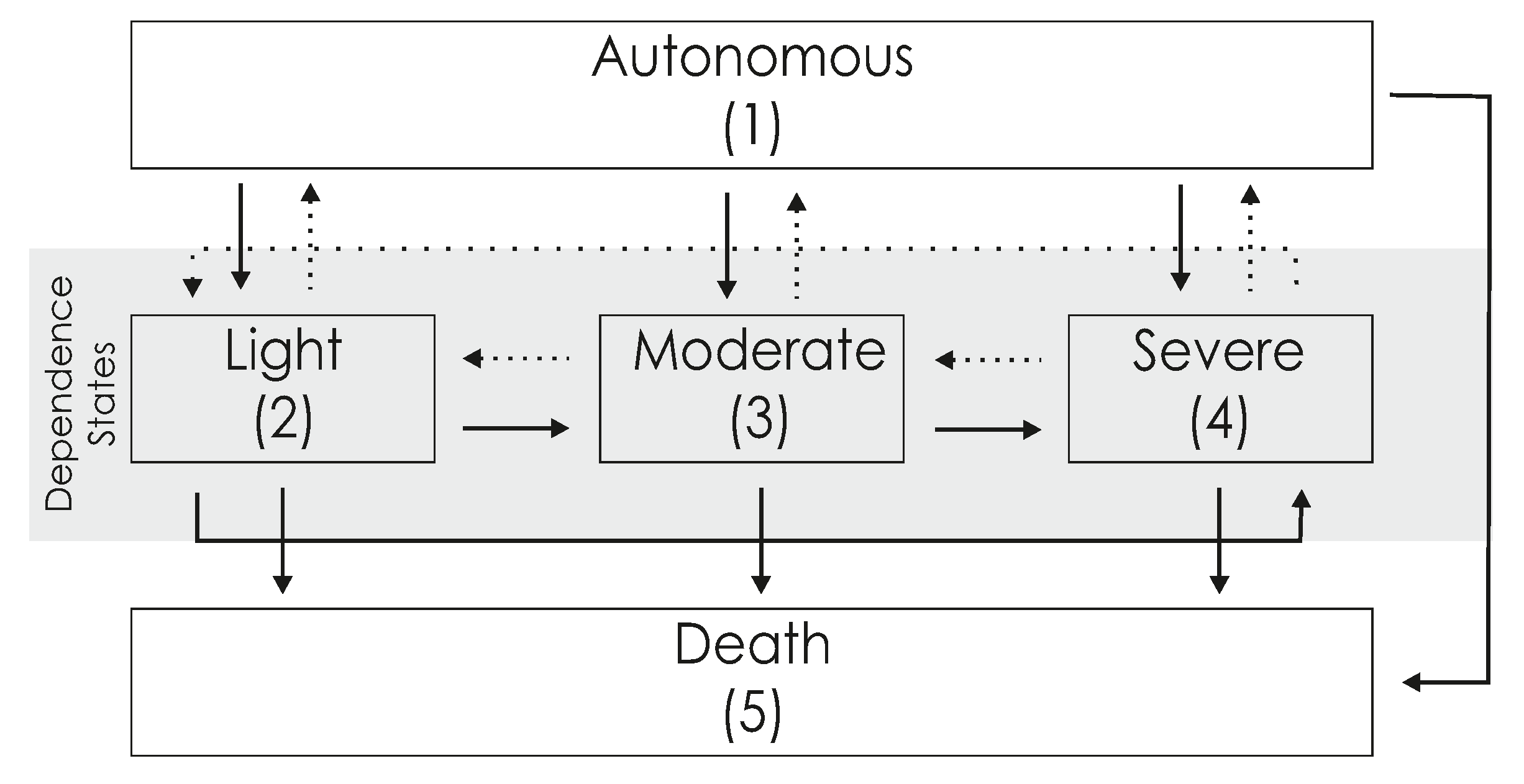
In this paper, we consider a five state non-homogeneous continuous time Markov model with one autonomous state, three dependent states and one exit state, namely states 1≡autonomous, 2≡light dependence, 3≡moderate dependence, 4≡severe dependence and 5≡death. The choice of the five state model is loosely justified by the widespread use of a reduced Barthel index, see (Mahoney and Barthel 1965), allowing for a general classification of elders in roughly three states of dependence, according to the performance achieved on their daily tasks. In order to obtain a general model, we allow for the transitions between all dependence states, as illustrated in Figure 1. Naturally, our methodology may be applied to other classification schemes and/or a multi-state model with a different set of transitions.
As for the mathematical approach, we follow the Transition Intensities Approach (TIA) which is vehemently advocated in (Waters 1984) and followed by several of the above cited authors. The transition intensities are key parameters in multi-states models as they reflect the dynamics of the underlying processes that shape an individual trajectory through dependence states during elderly ages. All the other corresponding characteristics of the Markov process and the evolution through the LTC model can, generally, be determined if the transition intensities are known, see for instance, (Haberman and Pitacco 1998) and (Waters 1984).
The first goal of this paper is to propose a method of obtaining transition intensities between dependence states by calibration with discrete time transition probabilities estimated from available data. This first goal intends to provide a method for obtaining transition intensities when only discrete time transition probabilities are available, as is the case in this paper. We illustrate the proposed methodology, obtaining transition intensities for the Portuguese population, using data from 2015, of the Portuguese National Network of Continuous Care Database. We believe this will bring valuable information for insurers, practitioners and institutions. For that, we adopt intensities of the form of the hazard function for the Gompertz-Makeham law, as in (Haberman and Pitacco 1998), and we propose a loss function that allows us to calibrate transition intensities from transition probabilities previously estimated from data.
Following TIA, the transition probabilities of the multi-state model are determined from the intensities by numerical integration of the Kolmogorov forward differential equations. The numerical integration is mandatory as, for the model presented in Figure 1, there is no evident closed form solution to the Kolmogorov equations (see Remark 2 ahead). We note that the numerical integration is not a severe limitation to our purposes and methods.
As a second goal we intend to simulate the cost of LTC in Portugal and for that, we use the continuous time transition probabilities derived from the Kolmogorov equations and we use Monte Carlo simulation in order to obtain, for a representative sample of trajectories of the Markov chain, the sojourn times in each state and the associated costs of LTC. These costs, in turn, will allow for the determination of insurance premiums and sojourn times in the system. These sojourn times may give us a a posteriori validation of the methodology by comparing them with the life expectancy of the official mortality table of the Portuguese Institute of Statistics, see (INE 2015), and the healthy life expectancy in Portugal, see (Pordata 2016b). Other authors, see (van den Hout et al. 2014) for instance, have already used multi-state models to predict healthy life expectancy.
The general methodology proposed in this paper will allow for future calibration of intensities if the population’s characteristics change or to obtain transition intensities for smaller populations, such as LTC insurance portfolios or even for different schemes of LTC products.
2. Context and Notations
Let denote the continuous time Markov process describing, in each realization, the path of an individual through the different states i of his health condition, with . For each , the random variable takes one of the values in and the event indicates that the individual is in state i at time t.
For states i and j of the continuous time Markov chain and for , we have:
- The transition probabilities, for an individual aged x, defined by:i.e., is the probability that an individual aged x in state i will be in state j at age . So we havethat is, the matrix is stochastic.
- The sojourn probabilities, for an individual aged x, given byi.e., is the probability that an individual aged x in state i stays in state i throughout the whole period from age x to age .
As a consequence of the Markov property, the transition probabilities satisfy the Chapman- Kolmogorov equations
and, also, the sojourn probabilities satisfy
In the so called Transition Intensity Approach (TIA) we want to determine the transition probabilities from the transition intensities , for , with
Remark 1.
Let us stress that if, for , we have then obviously ; but, more important for our purposes ahead, we may have and for some ; in this case, we only have that the slope at zero of , as a function of h, is null.
We may define the (total) intensity of decrement from state , as reflecting the conditional probability of leaving state i over an infinitesimal interval given that the process is in state i at time (age) x, by:
The Kolmogorov forward ordinary differential equations (with corresponding boundary conditions), for all states and , given by
are a consequence of the Chapman-Kolmogorov Equations (1). For the sojourn probabilities there is also an equation that can be easily derived by
from where we can obtain:
In matrix notation, see (Ross 1996), the system of equations (3) may be written as:
by considering the intensity matrix
For that, just observe that the term with indexes , corresponding to the matrix product is given by:
that is, exactly, the Kolmogorov forward Equations (3).
Remark 2.
In the case of constant intensities, the solution of equations (4) are obtained by a direct integration amounting to the computation of a matrix exponential. In the general case, for every x, the Kolmogorov equations (4) are a system of linear equations with an matrix, , with regular coefficients. For intensities in which we do not have, for every , , we cannot guarantee the existence of a solution obtained by direct integration (see Ver Eecke 1985, p. 146), and that is the case of the model treated in this work. Nevertheless, general results ensure the existence of a unique solution with good properties, see (Teschl 2011) or (Ver Eecke 1985, p. 141), and by numerical integration, as performed in this work, these solutions can be determined in a form suitable for many other computational purposes.
3. Modeling Transition Rates
In the absence of a developed market of LTC insurance products, as is the case in Portugal, it may be hard to find quality data allowing the statistical estimation of the parameters of the model, namely in the TIA approach, the intensities parameters. Nevertheless, in the case of having some information on the state transitions allowing for the estimation of a discrete time homogeneous Markov chain model, we will now show that it is possible to calibrate the non-homogeneous continuous-time model to the discrete time one.
Our methodology of modeling transition rates relies on the following idea: (i) Using real data and a multi-state model, estimate discrete time probabilities, which will be used to calibrate continuous-time transition rates; (ii) Adopting a hazard type transition intensities and choosing a given starting age x, derive a numerical solution for the Kolmogorov differential equations, in order to obtain the transition probabilities given by the continuous time multi-state model; (iii) Using an optimization criteria, calibrate the transition intensities parameters in order to meet the n-step discrete time transition probabilities estimated from data; (iv) Finally, using sojourn times of the multi-state model, assess the quality of the calibration with the obtained life expectancy for age x, by comparison with the official life expectancy and by the sojourn time of the autonomous state by comparison with official healthy life expectancy at age x. In our case, these indicators are both available for Portuguese population, see (INE 2015) and (Pordata 2016a).
In our formulation, following (Haberman and Pitacco 1998, p. 25), we consider variable intensity rates of Gompertz-Makeham type, of the form:
for some sets and B. For each pair of states , we define the set of parameters to calibrate by .
Although specific data from this regard is lacking, such hypothesis seems reasonable. We note that, in the proposed methodology, other types of transition intensities may be efficiently adopted, such as in (Olivieri and Pitacco 2000), for instance.
We note that assumption (5) is equivalent to consider variable intensity matrices in Equation (4), with (non diagonal) entries of the form
for some sets and B. For and B closed bounded intervals we have that the parameter set defined by:
being a product of compact real intervals is compact. We will identify the set of all sets of admissible intensities of interest, say , with . Therefore, to any such element of such a set of admissible intensities , there corresponds univocally an intensity matrix .
Since we only have access to estimated transition probabilities, we consider (5) a reasonable and general assumption. We note, however, that the proposed methodology applies to other types of intensity rates.
Model Calibration via an Optimization Problem
In this section, we will show the existence and uniqueness result of the calibration of transition intensities with data.
Theorem 1.
Let, for and a fixed initial age , be a sequence of transition matrices for homogeneous Markov LTC models and for any set of intensities , the correspondent matrix of transition probabilities for the same reference age x. Consider the loss function
Then, for the optimization problem there exists such that,
the unique minimum being attained at possibly several points .
Proof.
As we suppose that is compact, we just have to show that, for every fixed t, is a continuous function of . Recall that considering the dependence of the matrix on its entries and, of those on the parameters, Equation (3) may be written as
an equation that can be read in integral form as:
We will now follow the general idea of the proof of the Picard–Lindelöf theorem for proving existence and unicity of solutions of ordinary differential equations as exposed for the backward Kolmogorov equations in (Rolski et al. 1999, pp. 348–49). By replacing in the righthand member of Equation (8) by this righthand member we obtain,
and, by mathematical induction, we have
Now, let . As being continuous is integrable over any compact set, by Lemma 8.4.1 in (Rolski et al. 1999, p. 348), we have that
Finally, since
we have that the series which sum represents , that is
is a series of continuous functions of the parameter converging uniformly and so the sum is a continuous function of the parameter . □
As expected, having as a compact set, the previous theorem ensures the existence of an optimal calibration under the objective function in Formula (6).
We note that the proposed methodology corresponds to a minimum square error criteria, a common approach in this kind of problems. We will choose the set of intensities that minimizes the loss function (6), thus ensuring a calibration of the intensities to real data.
Remark 3.
Despite the fact that the optimization problem defined by Formula (6) has a unique solution, the effective computation of this solution most probably is a hard problem for two different reasons. The first reason is that, in our model, there are three parameters for each intensity and a total of 16 intensities, which amounts to an optimization problem in a space of 48 variables. Such high dimensionality has an implicit a priori challenge (see, for instance (Grosan and Abraham 2009)). The second reason, coupled with the first reason just mentioned, is that the function to be optimized depends on the parameters by the computation of the transition probability functions, using numerical integration. Being so, it seems justified to employ a simple calibration approach to the determination of the parameters, such as the one presented below.
Setting an initial age , a time horizon N and considering transition intensities ruled by Equation (3), and considering the model framework represented in Figure 1, we calibrate the transition intensities for each pair of states , in order to fit the one step transition probabilities estimated from data.
In a first step, consider baseline parameters for intensities and , representing the transition intensities from autonomous to light dependence and from autonomous to death, respectively. We propose, as a starting point, the ones assumed in (Haberman and Pitacco 1998, p. 100), namely:
In a second step, considering , the one step probability of an individual aged x moving from state i to state j (estimated from data) and the fine tuning parameters chosen to reduce the loss function in Formula (6), we perturb the parameters illustrated in (9) in order to reflect the structure of the one step transition estimated matrix, by the transformations presented in the following:
- Parameters :
- Parameters :
- Parameters :
The reasoning behind the perturbation method in Formulas (10)–(12) is to slightly alter the classical intensities in order to coherently reflect the structure of each of the discrete transition matrices obtained from Portuguese data, thus reflecting the structure of the transitions in the population under study.
In a third step, we obtain the different transition probability functions, , as a result of numerically solving the Kolmogorov forward differential Equations (4) and we calibrate the transition intensities by finding (, , ) that minimizes the loss function (6).
We note that, from a practical point of view, and for the model framework presented in Figure 1, it means that we consider transition probabilities in order to obtain a small value for the loss function , defined in (6).
The proposed transformations are general and applicable to any population data and reduces the minimization problem of loss function (6) from a set of 48 parameters, , to only 3, namely .
The goal at this stage is to have the intensities parameters to reflect the structure of the data inferred matrices. By reducing the complexity of the optimization problem, it becomes more robust and easier to manage.
4. Outcomes from Portuguese Data
Using data from the Portuguese National Network of Continuous Care, we illustrate the obtained results for the methodology presented in this paper. The database for 2015 contains 23,894 users and a total of 93,134 records of observations. For some more details on the Portuguese LTC database, see again (Lopes et al. 2018a) and (Lopes et al. 2018b).
4.1. The Transition Probability Matrix
In this section, we present the discrete time one step probability matrix, obtained from the RNCCI database, by a clustering analysis, as described in (Oliveira et al. 2017), for a set of states and transitions defined in Figure 1. This one step transition matrix will be used in the calibration process for obtaining intensity rates.
Observing the estimated homogeneous matrix (13), for ages over 60 years old, we highlight that: (i) for each dependence state, the higher probabilities correspond to maintaining the same dependence level in one step (one year); (ii) the rates of mortality increase with the dependence level; (iii) we observe non-null transition probabilities between all dependence levels.
For illustration purposes, in Table 1, we present the transition matrices obtained for different sets of ages, estimated from the same database in (Oliveira et al. 2017), and matrix , already presented in (13), obtained by a convex combination of the other ones, according to the proportion of individuals in RNCCI for each age group.
The above comments over the structure of the one step transition matrix for the whole database remain valid when we focus only on a shorter set of ages. Moreover, analysing the set of transition matrices of Table 1, we can conclude that non-homogeneous transition intensities are more adequate to model the LTC phenomena, since there are significant differences between the magnitude of transition probabilities over different levels of dependence, as age increases.
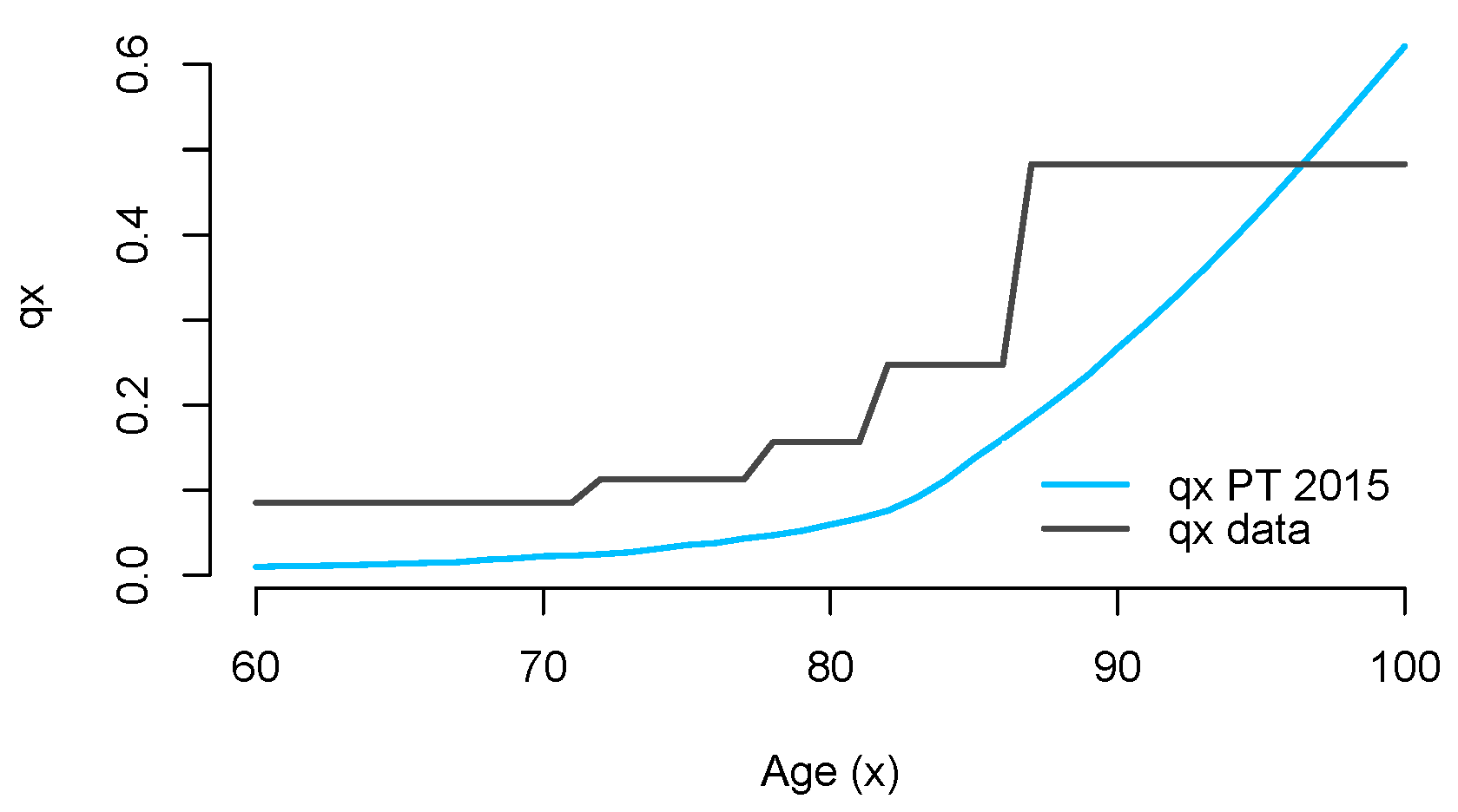
Figure 2 illustrates the mortality rates for each age for the Portuguese population in 2015, see INE (2016), in comparison with the mortality rates for the population under study on this section. These mortality rates were estimated from matrices on Table 1 and from distribution of RNCCI patients through dependence levels, presented in Table 2.
With
Table 2 illustrates the initial distribution of individuals, for the whole population and at age 65, through the dependence states, in the RNCCI database of 2015.
4.2. Calibrated Intensity Rates
Setting an initial age , a time horizon and considering transition intensities ruled by Equation (3), we calibrated the transition intensities for each pair of states , in order to fit the Portuguese transition probabilities illustrated in transition matrix (13).
Considering the baseline parameters defined in (9) and the one step transition probabilities represented in (13), we performed the transformations (10), (11) and (12).
In Table 3 we present the values of the mean error for each probability corresponding to some choices of the fine tuning parameters .
Taking the set , as our best choice of parameters, we present, in Table 4, the calibrated parameters for the intensities used in the simulation, which reflects a mean error of in the approximation of the transition probability functions by the estimated discrete transition probabilities.
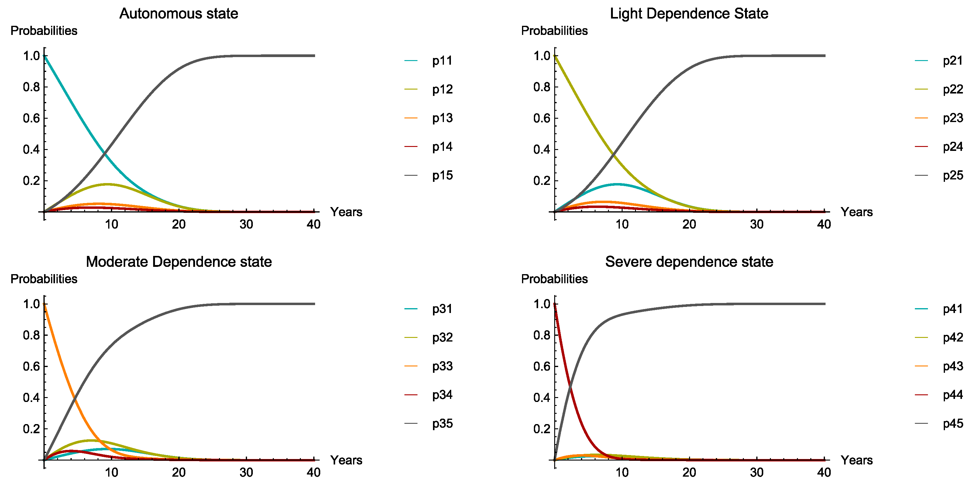
Figure 3 illustrates the transition probability functions for a 65 year old individual, obtained by numerical integration of the Kolmogorov forward differential equations.
Remark 4.
A natural question related to the proposed calibration method is to determine if the relation between the transition matrix used for calibration and the continuous time probability transition matrix obtained by integrating the Kolmogorov equations with the calibrated intensities corresponds–in some sense–to the solution of the imbedding problem for finite Markov chains (see, for instance, (Kingman 1962), (Johansen 1973) and (Johansen 1974)). In the imbedding problem we seek to determine the existence of a continuous time Markov chain transition probability matrix corresponding to a discrete time probability transition matrix that represents the observation of the continuous time Markov chain at unit intervals of time. We observe that in the case where is a solution to the imbedding problem of a one step Markov chain probability transition matrix, then with the n-step probability transition matrix we should have in Formula (6), .
5. Simulation Procedure and Results
After calibrating the transition intensities and integrating the Kolmogorov forward differential equations, we simulate 10,000 trajectories of the continuous time Markov chain in order to obtain significant information over the LTC population in Portugal.
The simulation algorithm used, which is tantamount to a simulation of a continuous time Markov chain, is presented in Algorithm 1.
| Algorithm 1: Algorithm of the Simulation. |
1: INPUT Kolmogorov equations solutions ; ; 2: ; 3: 4: 5: ; 6: WHILE (Age < Max Age) ∧ (State < 5) 7: 8: 9: 10: 11: , 12: 13: REPEAT 14: PRINT U |
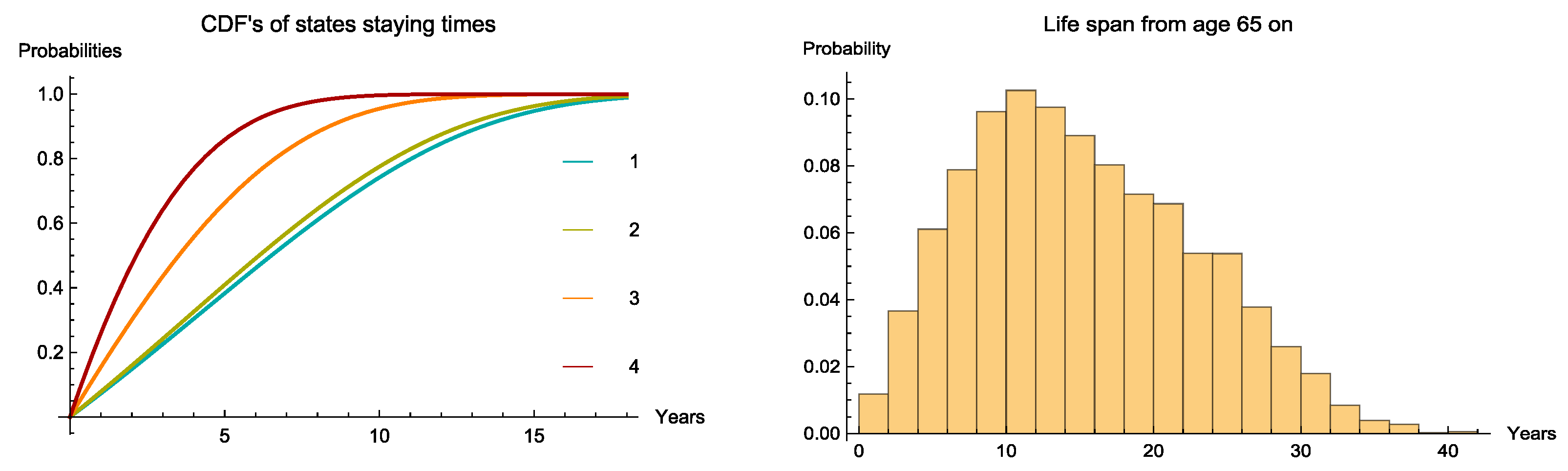
With the simulation process, we obtained information on the sojourn times distribution, illustrated in the left side of Figure 4; the life expectancy at age , see the right side of Figure 4 and obtained statistical measures for the whole life cost of Long Term Care, by considering a set of reasonable monthly costs for each dependence level, see Figure 5.
5.1. Sojourn Times and Life Expectancy
The simulation procedure requires the probability distribution functions of the sojourn in each transient state , which are obtained by the calibrated intensity rates, by numerical integration of the Kolmogorov forward differential equations. The cumulative distribution functions are displayed in the left side of Figure 4.
Table 5 illustrates the average sojourn times for each dependency level, for a 65 year old individual. The “life expectancy” in Table 5 corresponds to the average sum of all sojourn times, , before the individual deceases.
We note that the life expectancy given by the official 2015 mortality tables of the National Institute of Statistics in Portugal, see (INE 2015), for a 65 year old PortugPortugueseuese, is 19.19, which reflects that our estimate has a relative difference of −20.74% compared to the official data. According to the recent results on (Bravo et al. 2020), the 95% confidence interval for the life expectancy of Portuguese individuals that, in 2015, were 65 year old is . In our opinion, the magnitude of this relative difference is explained by the the observation of Figure 2. We note that the population in RNCCI system is mostly a population with comorbidities, which induces higher mortality and, as a consequence, reduces the life expectancy. We remark that we are considering a sub-population of Portuguese individuals that, during 2015, used the National Network of Continuing Care. In fact, as presented in Table 2, 55.22% of the individuals aged 65 were registered as light dependent level and 22.64% as severe dependent. We believe that in the general Portuguese population these percentages are not so high, and this justifies that we observe a lower life expectancy. As a second benchmark, we note that the official Healthy Life years at age 65, in Portugal, in 2015, was 7 years, see (Pordata 2016a). In that sense, we consider our results a reasonable approximation and it gives us a validation for the calibration procedure and results. We also remark that during the simulation procedure, different scenarios have been tested (different ages structure in the population, different initial distributions for the 65 year old individuals) and all of them producing results consistent with the defined scenarios. Our option, in the paper, relied on presenting only the results obtained from the RNCCI database.
We present, in the right side of Figure 4, the empirical distribution for the life expectancy for a 65 year old Portuguese, obtained in the simulation process.
We remark that it is possible to obtain similar results for other initial ages, rather than , given that transition rates are calibrated for other ages x as well as for other age structure populations, obtaining a new one step transition matrix from an appropriate convex combination of the matrices presented in Table 1.
We note that, for the population under study, if we had chosen to calibrate the intensities and present the results for the mean age of RNCCI database (80 years old), the differences would be smaller. However, for instance, the Healthy Life years at age 80 is not available for comparison with our results. In that sense, our choice relied on calibrating the intensities for age 65.
5.2. Simulating the Costs of LTC
The protection of individuals in later stages of life can be financed by social protection, by insurance policies or a combination of both.
At this point, we intend to obtain, by simulation procedures, the distribution of costs of LTC for a population with the characteristics of RNCCI users, as well as some basic illustrative statistics.
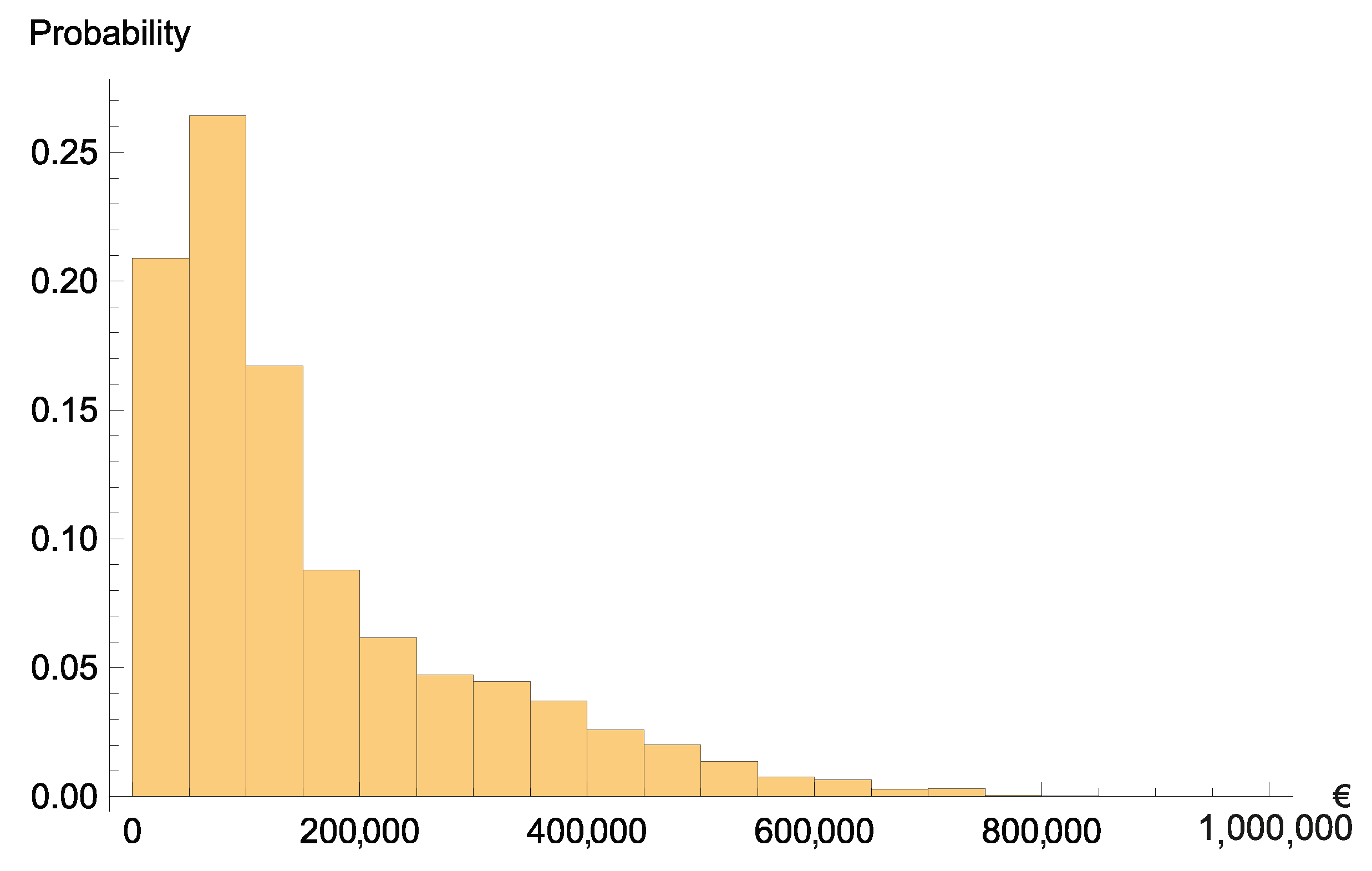
The presented results were achieved by admitting that the monthly cost for users in each of the dependent states is, respectively, 500, 1 500 and 3 000 euros. These values are of the same magnitude of the expenditures per level of care reported in (Zuchandke et al. 2012, p. 221), for LTC in Germany in 2010. Figure 5 illustrates the distribution of LTC costs, under the monthly costs assumed, for a 65 year old individual.
The simulated average whole life cost of Long Term Care may be seen as the Risk Premium of an LTC insurance, if the same rates are used for increasing costs and discounting, or as an average amount per patient in social assistance institutions. Regarding the skewness of the distribution, we note that, for insurance purposes, the risk measurement and the premium calculation should reflect this fact.
Table 6 highlights the Life Expectancy, the Risk Premium and the correspondent monthly equivalent investment, for a period of 30 years–i.e. starting to invest at the age of 35 years old, with a technical interest rate of 3%–necessary to face the global cost amount. We remark that, naturally, the methodology proposed in this paper allows for the simulation for other populations with different characteristics, namely for the general Portuguese population or for some insurance portfolios.
Just for illustration purposes, we show, in Table 7, the advantages of an early subscription over some kind of investment allowing for covering the amount of the Risk Premium of an expensive LTC contract. We illustrate, in line, different subscription ages x and, in column, different initial ages for entering in a LTC system. For each of these pairs (x, ) we calculated the monthly investments needed to face the global whole life LTC cost, according to the obtained simulations. The last line illustrates the “life expectancy” after age and the previous one shows the global average cost of LTC after that age.
We remark that, as previously referred, the values presented in Table 7 are not perfectly accurate for ages different than 65, since we used, for all ages , the calibrated transition intensities for a generic 65 year old individual. Despite less accurate, the results are still interesting and highlight the need for early investment on LTC coverages.
To conclude this section, we discuss the effect of the number of repetitions in the simulation process. We can appreciate in both Table 8 and Table 9 that there is no appreciable difference of the results both on the Risk Premiums computations and on the sojourn times among samples of 10,000 and 10,000 repetitions. As so, our choice of a sample of 10,000 trajectories for the discussion of the simulation results seems justified.
6. Conclusions
The calibration-simulation method introduced, allows for a study of insurance products and risk management of Long Term Care via a continuous time Markov chain model. The expected life span after age 65 (total life span and healthy life expectancy)–which is an output of the continuous time Markov chain simulation–is a good a posteriori validation tool for the proposed methods when comparing it to data from the official Portuguese mortality tables. We observe that, in our work, we obtained results of the same order of magnitude as those observed in the German LTC system, for similar input values of monthly costs. The calibration procedure proposed is efficient although it does not necessarily ensure a global optimum of the natural loss function. We point out some limitations of our study that opens opportunities for future work. Namely, taking advantage of having data matrices for five age classes would allow for using, in the simulation process, different probability distributions according to the age at a certain point in time of the trajectory being simulated. A second determinant line of work would be to achieve a performant algorithm to the calibration global optimization problem referred in Remark 3.
Some new developments may also arise by considering semi-Markov process modeling, provided the available data to perform such modelling.
Author Contributions
These authors contributed equally to this work. All authors have read and agreed to the published version of the manuscript.
Funding
This work was partially supported through the project of the Centro de Matemática e Aplicações, UID/MAT/00297/2020 financed by the Fundação para a Ciência e a Tecnologia (Portuguese Foundation for Science and Technology). The APC was funded by Future HealthCare.
Institutional Review Board Statement
Not applicable.
Informed Consent Statement
Not applicable.
Acknowledgments
This work was published with financial support from Future HealthCare. The authors would like to thank Future HealthCare for their interest in the development of LTC in Portugal and for the essential financial support for the publication of this work.
Conflicts of Interest
The authors declare no conflict of interest.
References
- Bravo, Jorge, Mercedes Ayuso, Robert Holzmann, and Edward Palmer. 2020. Addressing the Life Expectancy Gap in Pension Policy. Insurance: Mathematics and Economics. in press. [Google Scholar]
- Christiansen, Marcus. 2012. Multistate models in health insurance. AStA Advances in Statistical Analysis 96: 155–86. [Google Scholar] [CrossRef]
- Cordeiro, Isabel. 2002a. A multiple state model for the analysis of permanent health insurance claims by cause of disability. Insurance Mathematics & Economics 30: 167–86. [Google Scholar]
- Cordeiro, Isabel. 2002b. Transition intensities for a model for permanent health insurance. Astin Bulletin 32: 319–46. [Google Scholar] [CrossRef] [Green Version]
- Costa-Font, Joan, and Christophe Courbage. 2012. Financing Long-Term Care in Europe: Institutions, Markets and Models. London: Palgrave Macmillan. [Google Scholar]
- de Castries, Henri. 2009. Ageing and Long-Term Care: Key Challenges in Long-Term Care Coverage for Public and Private Systems. The Geneva Papers on Risk and Insurance. Issues and Practice 1: 24–34. [Google Scholar] [CrossRef]
- Dickson, David, Mary Hardy, and Howard Waters. 2013. Actuarial Mathematics for Life Contingent Risks. Cambridge: Cambridge University Press. [Google Scholar]
- Fleischmann, Anselm. 2015. Calibrating intensities for long-term care multiple-state Markov insurance model. European Actuarial Journal 5: 327–54. [Google Scholar] [CrossRef]
- Fong, Joelle, Adam Shao, and Michael Sherris. 2015. Multistate Actuarial Models of Functional Disability. North American Actuarial Journal 19: 41–59. [Google Scholar] [CrossRef]
- Fuino, Michel, and Joël Wagner. 2018. Long-term care models and dependence probability tables by acuity level: New empirical evidence from Switzerland. Insurance: Mathematics and Economics 81: 51–70. [Google Scholar] [CrossRef]
- Grosan, Crina, and Ajith Abraham. 2009. A novel global optimization technique for high dimensional functions. International Journal of Intelligent Systems 24: 421–40. [Google Scholar] [CrossRef] [Green Version]
- Guillén, Monserrat, and Jean Pinquet. 2008. Long-Term Care: Risk Description of a Spanish Portfolio and Economic Analysis of the Timing of Insurance Purchase. The Geneva Papers on Risk and Insurance-Issues and Practice 33: 659–72. [Google Scholar] [CrossRef] [Green Version]
- Haberman, Steven, and Ermanno Pitacco. 1998. Actuarial Models for Disability Insurance. Boca Raton: Chapman & Hall/CRC. [Google Scholar]
- Helms, Florian, Claudia Czado, and Susanne Gschlößl. 2005. Calculation of LTC premiums based on direct estimates of transition probabilities. Astin Bulletin 35: 455–69. [Google Scholar] [CrossRef] [Green Version]
- INE. 2015. Complete Life Tables Portugal–2013–2015. INE-Statistics Portugal. Available online: https://www.ine.pt (accessed on 15 December 2020).
- INE. 2016. Resident Population. INE-Statistics Portugal. Available online: https://www.ine.pt (accessed on 15 December 2020).
- Johansen, Søren. 1973. A central limit theorem for finite semigroups and its application to the imbedding problem for finite state Markov chains. Zeitschrift für Wahrscheinlichkeitstheorie und Verwandte Gebiete 26: 171–90. [Google Scholar] [CrossRef]
- Johansen, Søren. 1974. Some results on the imbedding problem for finite Markov chains. Journal of the London Mathematical Society. Second Series 8: 345–51. [Google Scholar] [CrossRef]
- Kessler, Denis. 2008. The Long-Term Care Insurance Market. The Geneva Papers on Risk and Insurance. Issues and Practice 33: 33–40. [Google Scholar] [CrossRef]
- Kingman, John. 1962. The imbedding problem for finite Markov chains. Zeitschrift für Wahrscheinlichkeitstheorie und Verwandte Gebiete 1: 14–24. [Google Scholar] [CrossRef]
- Lopes, Hugo, Céu Mateus, and Cristina Hernández-Quevedo. 2018. Ten Years since the 2006 Creation of the Portuguese National Network for Long-Term Care: Achievements and Challenges. Health Policy 122: 210–16. [Google Scholar] [CrossRef]
- Lopes, Hugo, Céu Mateus, and Nicoletta Rosati. 2018. Impact of long term care and mortality risk in community care and nursing homes populations of the Portuguese National Network for Long-Term Care: Achievements and Challenges. Archives of Gerontology and Geriatrics 76: 160–68. [Google Scholar] [CrossRef] [Green Version]
- Mahoney, Florence, and Dorothea Barthel. 1965. Functional evaluation: The Barthel Index. Maryland State Medical Journal 14: 56–61. [Google Scholar]
- Mitchell, Olivia, John Piggott, and Satoshi Shimizutani. 2008. An Empirical Analysis of Patterns in the Japanese Long-Term Care Insurance System. The Geneva Papers on Risk and Insurance. Issues and Practice 33: 694–709. [Google Scholar] [CrossRef] [Green Version]
- OECD. 2019. Elderly Population (Indicator). Paris: OECD Publishing. [Google Scholar]
- OECD & European Union. 2013. A Good Life in Old Age? Paris: OECD Publishing. [Google Scholar]
- Oliveira, Matilde, Manuel Leote Esquível, Susana Nascimento, Hugo Lopes, and Gracinda Rita Guerreiro. 2017. Estimation of Markov transition probabilities via clustering. Proceedings of the Symposium on Big Data in Finance, Retail and Commerce 1: 85–90. [Google Scholar]
- Olivieri, AnnaMaria, and Ermanno Pitacco. 2000. Facing LTC Risks. In Proceedings of the XXXII International ASTIN Colloquium. Ottawa: International Actuarial Association. [Google Scholar]
- Pordata. 2016a. Contemporary Portugal Database: Life Expectancy at 65 Years Old: Total and by Sex. Available online: https://www.pordata.pt/en/Portugal/Life+expectancy+at+65+years+old+total+and+by+sex+(base+three+years+from+2001+onwards)-419 (accessed on 1 July 2019).
- Pordata. 2016b. Contemporary Portugal Database: Healthy Life Years at 65. Available online: https://www.pordata.pt/en/Europe/Healthy+life+year+at+65+by+sex-1590 (accessed on 1 July 2019).
- Rolski, Tomasz, Hanspeter Schmidli, Volker Schmidt, and Jozef Teugels. 1999. Stochastic Processes for Insurance and Finance. Wiley Series in Probability and Statistics; Chichester: John Wiley & Sons Ltd. [Google Scholar]
- Ross, Sheldon. 1996. Stochastic Processes. Wiley Series in Probability and Statistics: Probability and Statistics; New York: John Wiley & Sons Inc. [Google Scholar]
- Teschl, Gerald. 2011. Ordinary Differential Equations and Dynamical Systems. Graduate Studies in Mathematics. Providence: American Mathematical Society. [Google Scholar]
- van den Hout, Ardo, Ekaterina Ogurtsova, Jutta Gampe, and Fiona Matthews. 2014. Investigating healthy life expectancy using a multi-state model in the presence of missing data and misclassification. Demographic Research 30: 1219–44. [Google Scholar] [CrossRef] [Green Version]
- Ver Eecke, Paul. 1985. Applications du Calcul Différentiel. Paris: Presses Universitaires de France. [Google Scholar]
- Waters, Howard. 1984. An approach to the study of multiple state models. Journal of the Institute of Actuaries 111: 363–74. [Google Scholar] [CrossRef]
- Xie, Haifeng, Thierry Chaussalet, and Peter Millard. 2005. A continuous time Markov model for the length of stay of elderly people in institutional long-term care. Journal of the Royal Statistical Society. Series A. Statistics in Society 168: 51–61. [Google Scholar] [CrossRef]
- Zuchandke, Andy, Sebastian Reddemann, and Simone Krummaker. 2012. Financing Long-Term Care in Europe: Institutions, Markets and Models. Chapter: Financing Long term Care in Germany. London: Palgrave Macmillan. [Google Scholar]
Figure 1.
Illustration of the LTC model.

Figure 2.
Mortality rates - general population and RNCCI estimates.

Figure 3.
Transition probabilities given as numerical solutions of the Kolmogorov forward equations.
Figure 3.
Transition probabilities given as numerical solutions of the Kolmogorov forward equations.

Figure 4.
Sojourn CDF’s for autonoumous (1) and dependence states (2–4) (on the left) Life Span after age 65 (on the right).
Figure 4.
Sojourn CDF’s for autonoumous (1) and dependence states (2–4) (on the left) Life Span after age 65 (on the right).

Figure 5.
Simulated Global User Costs after age 65.


Table 1.
Homogeneous probability transition matrices.
Table 2.
Initial distribution of individuals in RNCCI database.
| Age | Dependence Level | |||
|---|---|---|---|---|
| Autonomous | Light | Moderate | Severe | |
| All Ages | 15.96% | 36.36% | 16.03% | 31.65% |
| Age 65 | 13.43% | 55.22% | 8.71% | 22.64% |
Table 3.
Mean error for each of the 800 probabilities in Formula (6), for several fine tuning parameters.
Table 3.
Mean error for each of the 800 probabilities in Formula (6), for several fine tuning parameters.
| 0.0004 | −0.00004 | −0.0002 | 17.87% |
| 0.00001 | −0.01 | −0.001 | 14.88% |
| 0.0000001 | −0.004 | −0.0001 | 10.64% |
| 0.00001 | −0.002 | −0.000001 | 9.68% |
Table 4.
Calibrated intensities parameters for RNCCI data.
| Dependence Level | i | j | |||
|---|---|---|---|---|---|
| 1 | 2 | 0.00040 | 0.060 | −5.46 | |
| Autonomous | 1 | 3 | 0.00043 | 0.054 | −5.46 |
| 1 | 4 | 0.00044 | 0.052 | −5.46 | |
| 1 | 5 | 0.00050 | 0.038 | −4.12 | |
| 2 | 1 | 0.00040 | 0.060 | −5.46 | |
| Light | 2 | 3 | 0.00042 | 0.056 | −5.46 |
| Dependence | 2 | 4 | 0.00043 | 0.054 | −5.46 |
| 2 | 5 | 0.00050 | 0.037 | −4.12 | |
| 3 | 1 | 0.00043 | 0.054 | −5.46 | |
| Moderate | 3 | 2 | 0.00039 | 0.061 | −5.46 |
| Dependence | 3 | 4 | 0.00040 | 0.061 | −5.46 |
| 3 | 5 | 0.00046 | 0.047 | −4.12 | |
| 4 | 1 | 0.00044 | 0.052 | −5.46 | |
| Severe | 4 | 2 | 0.00043 | 0.054 | −5.46 |
| Dependence | 4 | 3 | 0.00042 | 0.056 | −5.46 |
| 4 | 5 | 0.00042 | 0.054 | −4.12 |
Table 5.
Sojourn Times and Life Expectancy for , 10,000 Simulations.
| Dependence Level | Autonomous | Light | Moderate | Severe | Life Expectancy |
|---|---|---|---|---|---|
| Average Sojourn Time | 7.04 | 7.04 | 6.94 | 6.86 | 15.21 |
Table 6.
Simulation results (10,000 repetitions, ): Life expectancy, Average Whole Life LTC Costs (Risk Premium), Monthly Equivalent Investment over the last 30 years (3% interest rate) for a population with similar characteristics of RNCCI.
Table 6.
Simulation results (10,000 repetitions, ): Life expectancy, Average Whole Life LTC Costs (Risk Premium), Monthly Equivalent Investment over the last 30 years (3% interest rate) for a population with similar characteristics of RNCCI.
| Life Expectancy | Risk Premium | Monthly Investment |
|---|---|---|
| 15.21 | 155,657.00 euro | 209.10 euro |
Table 7.
Monthly Equivalent Investment (euro) for different initial ages.
| 65 | 70 | 75 | 80 | ||
|---|---|---|---|---|---|
| x | 30 | 209.10 | 121.86 | 65.31 | 36.14 |
| 35 | 265.99 | 152.13 | 80.41 | 44.02 | |
| 40 | 347.35 | 193.52 | 100.39 | 54.20 | |
| 45 | 471.51 | 252.72 | 127.70 | 67.66 | |
| 50 | 681.09 | 343.05 | 166.77 | 86.07 | |
| 55 | 1103.24 | 495.53 | 226.37 | 112.40 | |
| 60 | 2365.31 | 802.67 | 326.99 | 152.58 | |
| Global Cost | 155,657.00 | 113,249.00 | 74,731.00 | 50,369.10 | |
| Life Expectancy | 15.21 | 11.14 | 7.80 | 5.27 | |
Table 8.
Total Sojourn Times (“Life Expectancy”).
| Sample Size | 100 | 1 000 | 10,000 | 10,000 |
|---|---|---|---|---|
| Minimum | 1.47 | 0.33 | 0.06 | 0.07 |
| First Quartile | 10.46 | 8.92 | 9.29 | 9.37 |
| Median | 14.68 | 14.64 | 14.34 | 14.55 |
| Mean | 15.74 | 15.29 | 15.21 | 15.32 |
| Third Quartile | 21.78 | 21.09 | 20.65 | 20.79 |
| Maximum | 28.03 | 39.25 | 41.67 | 46.62 |
| Standard Deviation | 6.77 | 7.67 | 7.62 | 7.61 |
Table 9.
Statistics of whole life costs (euro), at age 65 years, for different sample sizes.
| Sample Size | 100 | 1000 | 10,000 | 10,000 |
|---|---|---|---|---|
| Minimum | 0.00 | 0.00 | 0.00 | 0.00 |
| First Quartile | 56,517.52 | 60,992.10 | 57,645.40 | 59,272.20 |
| Median | 104,248.00 | 110,722.00 | 106,454.00 | 108,156.00 |
| Mean | 177,888.00 | 168,390.00 | 155,657.00 | 158,250.00 |
| Third Quartile | 256,474.00 | 248,925.00 | 214,925.00 | 217,857.00 |
| Maximum | 716,023.00 | 863,529.00 | 995,460.00 | 1,230,000.00 |
| Standard Deviation | 178,435.00 | 155,921.00 | 144,814.00 | 147,626.00 |
Publisher’s Note: MDPI stays neutral with regard to jurisdictional claims in published maps and institutional affiliations. |
© 2021 by the authors. Licensee MDPI, Basel, Switzerland. This article is an open access article distributed under the terms and conditions of the Creative Commons Attribution (CC BY) license (http://creativecommons.org/licenses/by/4.0/).
Share and Cite
MDPI and ACS Style
Esquível, M.L.; Guerreiro, G.R.; Oliveira, M.C.; Corte Real, P. Calibration of Transition Intensities for a Multistate Model: Application to Long-Term Care. Risks 2021, 9, 37. https://0-doi-org.brum.beds.ac.uk/10.3390/risks9020037
AMA Style
Esquível ML, Guerreiro GR, Oliveira MC, Corte Real P. Calibration of Transition Intensities for a Multistate Model: Application to Long-Term Care. Risks. 2021; 9(2):37. https://0-doi-org.brum.beds.ac.uk/10.3390/risks9020037
Chicago/Turabian StyleEsquível, Manuel L., Gracinda R. Guerreiro, Matilde C. Oliveira, and Pedro Corte Real. 2021. "Calibration of Transition Intensities for a Multistate Model: Application to Long-Term Care" Risks 9, no. 2: 37. https://0-doi-org.brum.beds.ac.uk/10.3390/risks9020037
Note that from the first issue of 2016, this journal uses article numbers instead of page numbers. See further details here.